Incremental Proximal Multi-Forecast
Model Predictive Control

Abstract

Multi-forecast model predictive control (MF-MPC) is a control policy that creates a plan of actions over a horizon for each of a given set of forecasted scenarios or contingencies, with the constraint that the first action in all plans be the same. In this note we show how these coupled plans can be found by solving a sequence of single plans, using an incremental proximal method. We refer to this policy as incremental proximal model predictive control (IP-MPC). We have observed that even when the iterations in IP-MPC are not carried out to convergence, we obtain a policy that achieves much of the improvement of MF-MPC over single-forecast model predictive control (MPC).

1 Multi-forecast model predictive control

We consider a control policy which generates a control input $u_{t}\in{\mbox{\bf R}}^{m}$ from the current system state $x_{t}\in{\mbox{\bf R}}^{n}$ (presumed known), as well as other information that is available in (discrete time) period $t$.

1.1 Model predictive control

In model predictive control (MPC), we first form an approximation of the dynamics of the system over from period $\tau=t$ to period $\tau=t+H$, where $H$ is the planning horizon. The approximate dynamics are affine, of the form

$$x_{\tau+1}=A_{\tau|t}x_{\tau}+B_{\tau|t}u_{\tau}+c_{\tau|t},\quad\tau=t,\ldots,t+H-1.$$

Here $x_{t}$ is the current state, which is known; $x_{t+1},\ldots,x_{t+H}$ is our plan for the future states. The current control input (that we seek) is $u_{t}$; $u_{t+1},\ldots,u_{t+H-1}$ is our plan for future control actions. The data that define the dynamics used in our plan, $A_{\tau|t}$, $B_{\tau|t}$ and $c_{\tau|t}$, are a forecast or prediction, based on information known at period $t$. (These can change with $t$, as new information becomes available.) We let $x=(x_{t+1},\ldots,x_{t+H})$ and $u=(u_{t},\ldots,u_{t+H-1})$ denote the state and control action plans, respectively.

In MPC we choose the plan by solving the optimization problem

$$\begin{array}[]{ll}\mbox{minimize}&G_{t}(x_{t},x,u)\\ \mbox{subject to}&x_{\tau+1}=A_{\tau|t}x_{\tau}+B_{\tau|t}u_{\tau}+c_{\tau|t},\quad\tau=t,\ldots,t+H-1,\end{array}$$ (1)

with variables $x\in{\mbox{\bf R}}^{Hn}$ and $u\in{\mbox{\bf R}}^{Hm}$, where $G_{t}:{\mbox{\bf R}}^{n}\times{\mbox{\bf R}}^{Hn}\times{\mbox{\bf R}}^{Hm}\to{\mbox{\bf R}}\cup\{\infty\}$ is a convex cost function.

Infinite values of $G_{t}$ are used to enforce constraints, such as $u_{\tau}\in\mathcal{U}_{\tau}$, a convex set of allowed control actions, or $x_{t+H}\in\mathcal{X}^{\text{term}}$, a convex set of allowed terminal states for our plan. Traditionally the cost function $G_{t}$ is separable across $(x_{\tau},u_{\tau})$, but it need not be; for example it could penalize a maximum excursion of the state or maximum actuator use over the horizon. Like the dynamics, the cost function $G_{t}$ can also depend on forecasts of unknown future quantities, based on information available at period $t$. The model predictive control problem (1) is convex, and readily solved [11], even in real time [72, 41, 66, 6, 20]. The total number of scalar variables in the MPC problem (1) is $H(m+n)$.

History.

MPC has a long history and large literature, and is widely used. Some early work is [56, 16, 25]; for more recent surveys see the papers [46, 30, 35, 73, 42, 1] or books [39, 28, 13, 55, 54]. Papers describing applications of MPC in specific areas include data center cooling [34], building HVAC control [2, 21], wind power systems [31], microgrids [32], pandemic management [15, 49], dynamic hedging [52], railway systems [24], aerospace systems [23], and agriculture [19]. With appropriate forecasting (which in many applications is very simple) and choice of cost function, MPC can work well, even though it does not explicitly take into account uncertainty in the dynamics and cost, or more precisely, since it is based on a single forecast of these quantities. (It does have recourse, however, since the forecasts and plans are updated in each time period.)

1.2 Multi-forecast model predictive control

There are many extensions of MPC that attempt to improve performance by taking into account uncertainty in the future dynamics and cost. Examples include robust MPC [14, 7], min–max MPC [53], tube MPC [43], and stochastic MPC [44, 29].

One particularly simple approach is multi-forecast MPC (MF-MPC) which replaces the single forecast of $G_{t}$, $A_{\tau|t}$, $B_{\tau|t}$, and $c_{\tau|t}$ used in MPC with multiple forecasts, all of which are considered plausible. We denote these as

$$G^{i}_{t},~{}A_{\tau|t}^{i},~{}B_{\tau|t}^{i},~{}c_{\tau|t}^{i},\quad\tau=t,\ldots,t+H-1,\quad i=1,\ldots,S,$$

where the superscript $i$ gives the forecast or scenario, and $S$ is the number of scenarios. We can also specify positive weights $w^{1},\ldots,w^{S}$ associated with these forecasts, which are often taken to be one. These multiple forecasts can be found several ways. Each could be a forecast using a different but reasonable method; or they can be samples from a statistical model of future values. In the latter case, options include Monte Carlo sampling [65], Monte Carlo sampling with importance sampling [26], pseudo-Monte Carlo sampling [12], or sigma points in unscented transform [33, §19]. The scenarios can also be constructed by hand. It is common to take scenario $i=1$ as the single forecast that would be used in basic MPC.

To find the desired control action $u_{t}$, we solve the following extension of the single-forecast MPC problem (1):

$$\begin{array}[]{ll}\mbox{minimize}&\sum_{i=1}^{S}w^{i}G_{t}^{i}(x_{t},x^{i},u^{i})\\ \mbox{subject to}&x_{\tau+1}^{i}=A^{i}_{\tau|t}x_{\tau}^{i}+B_{\tau|t}^{i}u_{\tau}^{i}+c_{\tau|t}^{i},\quad\tau=t,\ldots,t+H-1,\quad i=1,\ldots,S\\ &u^{i}_{t}=u_{t},\quad i=1,\ldots,S,\end{array}$$ (2)

with variables $x^{i}\in{\mbox{\bf R}}^{Hn}$, $u^{i}\in{\mbox{\bf R}}^{Hm}$, and $u_{t}\in{\mbox{\bf R}}^{m}$ (our control action). In MF-MPC we create $S$ different future state and action plans, each using its own forecast of cost and dynamics, and add the constraint that all plans must agree on the first action $u_{t}$. Like the MPC problem (1), the MF-MPC problem (2) is also convex, but it can be a large problem if $S$ is large, with a total number of scalar variables $SH(m+n)+m$.

History and related literature.

MF-MPC is a simple special case of many other methods for incorporating uncertainty and information patterns via multiple scenarios [27, 74, 47, 67, 38, 40, 58, 17]. In these papers (and others) a scenario tree is used to represent the evolution of uncertainty over time, with non-anticipativity constraints imposed so that inputs from the same tree node are equal. Such multi-stage problems can then be solved by methods such as nested Benders decomposition [10, 47], progressive hedging [59], progressive decoupling [58], scenario decomposition with alternating projections [17], to evaluate the policy. In this context, MF-MPC is the very special case where there the scenario tree consists of the root (the current period), and $S$ edges to the different scenarios at period $t+1$. In terms of stochastic control, the information pattern for which MF-MPC is optimal is one where there are only $S$ possible outcomes (the scenarios): When the first action is taken, the $S$ outcomes are known but which one will obtain or realize is not; after the first action is taken, which of the scenarios is realized is revealed.

The MF-MPC problem is a basic and standard two-stage stochastic programming problem; see, e.g., [62, 22] [45, §5]. In this context the first stage is referred to as the “here and now” decision and the second stage as the “recourse” actions. For linear two-stage programs there are several algorithms that decompose the problem into each scenario based on cutting plane techniques [71, 60, 64, 63, 51, 37, 61], and for convex (nonlinear) two-stage problem there are methods based on augmented Lagrangians and ADMM [59, 5] [48, §7.6].

In summary, neither MF-MPC nor special methods for solving the MF-MPC problem, which is a two-stage stochastic programming problem, are new.

1.3 This note

The point of this note is to describe a method for solving the MF-MPC problem (1) using an incremental proximal method, a sequential algorithm that in each iteration solves a problem similar to the single-forecast MPC problem (1). If these iterations are continued long enough, the method will converge to a solution of the MF-MPC problem. Of more practical interest, we have found that stopping the incremental proximal algorithm early, well before it has converged, we obtain a policy that works well in practice, yielding most or all of the benefits of MF-MPC over single-forecast MPC.

In this note we are not concerned with comparing MF-MPC with other control policies, or arguing that it is a good policy. Our only point is that MF-MPC can be (approximately) evaluated using an iterative method in which each iteration is essentially solving a (single forecast) MPC problem. Thus the MF-MPC policy can be evaluated by solving a sequence of MPC problems, each one asssociated with one scenario.

2 Incremental proximal model predictive control

2.1 Incremental proximal method

We define $F^{i}:{\mbox{\bf R}}^{m}\to{\mbox{\bf R}}\cup\{\infty\}$, $i=1,\ldots,S$, as the optimal value of the MPC problem in scenario $i$, as a function of the first action $u_{t}$. Specifically, $F^{i}(u_{t})$ is the optimal value of the problem

$$\begin{array}[]{ll}\mbox{minimize}&w^{i}G_{t}^{i}(x_{t},x^{i},u^{i})\\ \mbox{subject to}&x_{\tau+1}^{i}=A^{i}_{\tau}x_{\tau}^{i}+B_{\tau}^{i}u_{\tau}^{i}+c_{\tau}^{i},\quad\tau=t,\ldots,t+H-1\\ &u^{i}_{t}=u_{t},\end{array}$$

with variables $x^{i}$ and $u^{i}$. This is a convex function since it is the partial minimization of a convex function over some variables (here, $x^{i}$ and $u^{i}_{t+1},\ldots,u^{i}_{t+H-1}$) [11, §3.2.5]. In terms of $F^{i}$, the MF-MPC problem (2) can be expressed as the problem

$$\begin{array}[]{ll}\mbox{minimize}&\sum_{i=1}^{S}F^{i}(u_{t}),\end{array}$$ (3)

with variable $u_{t}\in{\mbox{\bf R}}^{m}$. (This is the same as the MF-MPC problem (2), after we optimize over the variables $x^{i}$ and $u^{i}_{t+1},\ldots u^{i}_{t+H-1}$.)

The incremental proximal method [9, 8] solves problems with the sum form in (3). In the $k$th iteration the updated iterate $u_{t}^{(k+1)}$ is the solution of the problem

$$\begin{array}[]{ll}\mbox{minimize}&\alpha_{k}F^{i_{k}}(u_{t})+\frac{1}{2}\|u_{t}-u_{t}^{(k)}\|_{2}^{2},\end{array}$$ (4)

where $u_{t}$ is the variable, and $\alpha_{k}>0$ is a step size. The sample index $i_{k}$ can be chosen in a cyclic order ($i_{k}=k\mod S$), or uniformly randomly drawn from the $S$ scenarios. The step sizes should be square summable but not summable, with a typical choice $\alpha_{k}=\alpha/(k+\beta)$, where $\alpha$ and $\beta$ are positive parameters. The update (4) is the proximal operator of $\alpha_{k}F^{i_{k}}$ [57, 36, 48], giving the method its name. (‘Incremental’ refers to the fact that the scenarios are handled separately, one in each iteration.)

Solving the problem (4) is the same as solving the problem

$$\begin{array}[]{ll}\mbox{minimize}&\alpha_{k}w^{i_{k}}G_{t}^{i_{k}}(x_{t},x,u)+\frac{1}{2}\|u_{t}-u_{t}^{(k)}\|_{2}^{2},\\ \mbox{subject to}&x_{\tau+1}=A_{\tau|t}^{i_{k}}x_{\tau}+B_{\tau|t}^{i_{k}}u_{\tau}+c_{\tau|t}^{i_{k}},\quad\tau=t,\ldots,t+H-1,\end{array}$$ (5)

where $u$ and $x$ are the variables. Solving this convex optimization problem gives $u_{t}^{(k+1)}$. The problem (5) is identical to the single forecast MPC problem, except for the addition of the proximal term $\frac{1}{2}\|u_{t}-u_{t}^{(k)}\|_{2}^{2}$. In many cases the cost function $G_{t}$ already includes a quadratic term in $u_{t}$, in which case the problem (5) has exactly the same form as the single forecast MPC problem. Thus the cost of carrying out each iteration of the incremental proximal method is essentially the same as the cost of evaluating a single forecast MPC policy. We refer to the policy obtained by running a fixed number of iterations of the update (5) as the incremental proximal model predictive control (IP-MPC) method.

Convergence.

While the convergence proof given in [9, §3] does not exactly cover our case here, it is readily modified to handle it, with a few additional assumptions. Suppose $G^{i}$ has the form

$$G^{i}(x_{t},x^{i},u^{i})=g^{i}(x_{t},x^{i},u^{i})+\mathbb{I}(u^{i}\in\mathcal{U}^{i})+\mathbb{I}(x^{i}\in\mathcal{X}^{i}),$$ (6)

where $g^{i}$ is a real-valued convex function, $\mathbb{I}$ is the indicator function, the set $\mathcal{X}^{i}$ is convex, and the set $\mathcal{U}^{i}$ is convex and bounded. In this case, with step sizes that are square summable but not summable, we can conclude that $u_{t}^{(k)}$ converges to a solution of the MF-MPC problem (2). To see this, observe that when $G^{i}$ satisfies (6), the corresponding $F^{i}$ is a sum of a real-valued function and the indicator function of a bounded set. Though the bounded set depends on $i$, while the constraint set in [9] does not, with a minor modification one can show that the same convergence conclusions hold.

While it is nice to know that if the iterations of IP-MPC were continued indefinitely, we would (asymptotically) solve the MF-MPC problem (2), an essential part of IP-MPC is that performs well (as a policy) even when it is terminated long before it has solved the MF-MPC problem (2) to high accuracy.

2.2 Mini-batch IP-MPC

A useful extension of IP-MPC uses multiple scenarios in each update, i.e., a minibatch of scenarios, rather than just one. Thus in each iteration we solve not a signle-forecast MPC problem but a smaller MF-MPC problem, with $b\ll S$ scenarios, where $b$ is the minibatch size.

In the $k$th iteration, we take a subset of indices $\mathcal{S}_{k}\subset\{1,\ldots,S\}$ with $|\mathcal{S}_{k}|=b$, which can be chosen cyclically or drawn randomly from the scenario indices, with or without replacement. Then the updated iterate $u_{t}^{(k+1)}$ is the solution of the problem

$$\begin{array}[]{ll}\mbox{minimize}&(\alpha_{k}/b)\sum_{i\in\mathcal{S}_{k}}F^{i}(u_{t})+\frac{1}{2}\|u_{t}-u_{t}^{(k)}\|_{2}^{2}\end{array}$$

with variable $u_{t}$, which is an MF-MPC problem with $b$ scenarios, plus the quadratic proximal term. This problem can be expressed as

$$\begin{array}[]{ll}\mbox{minimize}&(\alpha_{k}/b)\sum_{i\in\mathcal{S}_{k}}w^{i}G_{t}^{i}(x_{t},x^{i},u^{i})+\frac{1}{2}\|u_{t}-u_{t}^{(k)}\|_{2}^{2},\\ \mbox{subject to}&x_{\tau+1}^{i}=A_{\tau|t}^{i}x_{\tau}^{i}+B_{\tau|t}^{i}u_{\tau}^{i}+c_{\tau|t}^{i},\quad\tau=t,\ldots,t+H-1,\quad i\in\mathcal{S}_{k}\\ &u_{t}=u_{t}^{i},\quad i\in\mathcal{S}_{k},\end{array}$$

where the variables are $x^{i}$, $u^{i}$, for $i\in\mathcal{S}_{k}$ and $u_{t}$. The number of scalar variables is $bH(n+m)+m$, which is about $b$ times of that of the IP-MPC problem (5), and a factor $S/b$ smaller than the full MF-MPC problem (2).

As the minibatch size $b$ increases, the incremental proximal method converges faster (in terms of number of iterations), but the iterations are more costly. A good choice of $b$ trades off these two competing trends.

3 Example

In this section we illustrate IP-MPC with a simple energy storage arbitrage problem.

3.1 Problem and policies

The problem.

We are to choose the charging (discharging, when negative) rate of an energy storage system in each hour, with time-varying energy prices, so as to maximize our average profit. We let $u_{t}\in{\mbox{\bf R}}$ denote the battery charging rate in period (hour) $t$, and $q_{t}$ the stored energy. These must satisfy $-D\leq u_{t}\leq C$ and $0\leq q_{t}\leq Q$ for all $t$, where $D$ is the maximum discharge rate, $C$ is the maximum charge rate, and $Q$ is the storage capacity. The storage dynamics is given by $q_{t+1}=q_{t}+u_{t}$. The cost in period $t$ is given by $p_{t}(u_{t}+\eta|u_{t}|)$, where $p_{t}\geq 0$ is the mid-price and $\eta\in(0,1)$ gives a gap between the buy and sell prices, i.e., we purchase energy at higher price $(1+\eta)p_{t}$, and we sell it back at the lower price $(1-\eta)p_{t}$. The charging rate $u_{t}$ is chosen with knowledge of the current stored energy $q_{t}$ and current price $p_{t}$, but not future prices $p_{t+1},\ldots$, which, however, can be forecast. The goal is to minimize the average cost, i.e., to maximize the average profit.

In this problem the state is the stored energy $q_{t}$, and the actual system dynamics are linear, constant, and known. The true cost is convex, and in this case separable across periods. The only uncertainty is in the future energy prices, which affects the cost.

MPC policy.

We use a planning horizon $H=24$, i.e., one day. We denote the forecast of future prices as $\hat{p}_{\tau}$, $\tau=t+1,\ldots,t+23$. For notational simplicity, we use $\hat{p}_{t}=p_{t}$, the known current price. At time $t$, we plan the input $u_{\tau}$ from $\tau=t$ to $\tau=t+23$, i.e., we plan over the next 24 hours. To determine $u_{t}$ we solve the problem

$$\begin{array}[]{ll}\mbox{minimize}&\sum_{\tau=t}^{t+23}\left(\hat{p}_{\tau}u_{\tau}+\eta\hat{p}_{\tau}|u_{\tau}|\right)\\ \mbox{subject to}&-C\leq u_{\tau}\leq D,\quad\tau=t,\ldots,t+23\\ &0\leq q_{\tau}\leq Q,\quad\tau=t+1,\ldots,t+24\\ &q_{\tau+1}=q_{\tau}+u_{\tau},\quad\tau=t,\ldots,t+23\\ &q_{t+24}=Q/2,\end{array}$$

with variables $u_{t},\ldots,u_{t+23}$ and $q_{t+1},\ldots,q_{t+24}$. (The current stored energy $q_{t}$ is known.) The terminal constraint requires that in our plan, the terminal storage energy should be half the capacity.

MF-MPC policy.

We denote the $S$ forecasts of future prices as $\hat{p}_{\tau}^{i}$, $\tau=t+1,\ldots,t+23$, $i=1,\ldots,S$, with $\hat{p}_{\tau}^{1}$ the forecast used in MPC. As in MPC, we take $\hat{p}_{t}^{i}=p_{t}$, the known current price. We create plans $u_{\tau}^{i}$, $\tau=t,\ldots,t+23$, $i=1\ldots,S$, with the constraint that $u_{t}^{1}=\cdots=u_{t}^{S}$, with the common value giving us $u_{t}$. We solve the problem

$$\begin{array}[]{ll}\mbox{minimize}&(1/S)\sum_{i=1}^{S}\sum_{\tau=t}^{t+23}\left(\hat{p}_{\tau}^{i}u_{\tau}^{i}+\eta\hat{p}_{\tau}^{i}|u_{\tau}^{i}|\right)\\ \mbox{subject to}&-C\leq u_{\tau}^{i}\leq D,\quad\tau=t,\ldots,t+23,\quad i=1,\ldots,S\\ &0\leq q_{\tau}^{i}\leq Q,\quad\tau=t+1,\ldots,t+24,\quad i=1,\ldots,S\\ &q_{\tau+1}^{i}=q_{\tau}^{i}+u_{\tau}^{i},\quad\tau=t,\ldots,t+23,\quad i=1,\ldots,S\\ &q_{t+24}^{i}=Q/2,\quad i=1,\ldots,S\\ &u_{t}^{1}=\cdots=u_{t}^{S},\end{array}$$

with variables $u_{\tau}^{i}$, $\tau=t,\ldots,t+23$, $i=1,\ldots,S$, and $q_{\tau}^{i}$, $\tau=t+1,\ldots,t+24$, $i=1,\ldots,S$. We take $q_{t}^{i}=q_{t}$, the current known stored energy.

3.2 Parameters and data

Parameters.

We take $C=D=10$ and $Q=50$, so we can completely charge or discharge our storage system in $5$ hours. We take $\eta=0.075$, which means there is a 15% difference between the energy buy and sell prices.

Price data.

We use real price data, the hourly verified real-time local marginal price (LMP), in dollars per MWh, for zonal node 51217 obtained from the PJM market [50], over a period of $268$ weeks from July 2016 through August 2021. We clip or winsorize the smallest values at the 0.2-percentile of prices, which is $6.6$; the maximum price over this time period was $690$. The mean price is $28.5$, and the median price is $23.9$.

We use the data of the first $260$ weeks, from July 1 2016 to June 24 2021, to fit our forecasting model, and the data of the last $8$ weeks, June 25 to August 19 2021, to evaluate our policies. The prices are shown in figure 1, with blue showing the data used to develop our forecast model, and orange showing the price data used to evaluate the policies.

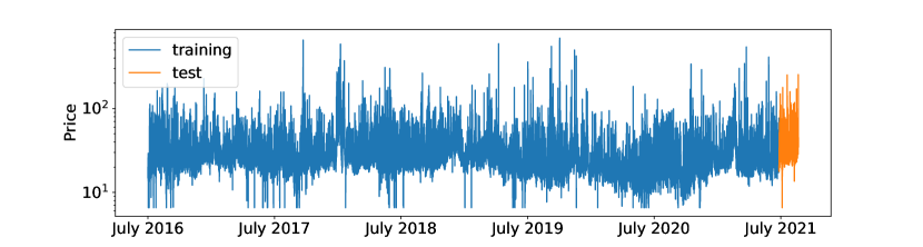
Figure 1: Electricity price $p_{t}$, in dollars per MWh, over $268$ weeks. Prices shown in blue are used to fit the forecasting models; the prices shown in orange are used to evaluate various policies.

3.3 Forecasts

Transformation.

The price data are very right skewed, so we first transform them with two log transforms, and work with $z_{t}=\log\log p_{t}$, which results in a distribution of values that is reasonably Gaussian. While our forecasting methods will use $z_{t}$, we convert our predictions (single or multiple) back to prices using $\hat{p}_{t}=\exp\exp\hat{z}_{t}$.

Baseline model.

We use the simple forecast method described in [45, §A], applied to $z_{t}$, which first fits a baseline to the price data that captures the daily, weekly, and seasonal variation. Our baseline $b_{t}$ has the form

$$b_{t}=\beta_{0}+\sum_{i=1}^{16}\left(\beta_{i}\cos(2\pi t/T_{i})+\alpha_{i}\sin(2\pi t/T_{i})\right),$$

where the model parameters are $\beta_{0}$, $\beta_{i}$ and $\alpha_{i}$ for $i=1,\ldots,16$. The periods $T_{i}$ are as follows.

• Diurnal (daily) variation: $T_{i}=24/k$, $k=1,2,3,4$

• Weekly variation: $T_{i}=7\times 24/k$, $k=1,2,3,4$

• Seasonal (annual) variation: $T_{i}=365\times 24/k$, $k=1,2,3,4$

• Interaction terms: $T_{i}=7\times 24\pm 24$, $365\times 24\pm 24$

Thus our basic daily, weekly, and seasonal variation models each have $4$ Fourier coefficients; the interaction terms allow the baseline daily and weekly patterns to vary (a bit) over the year.

Our baseline model has $33$ parameters; we fit these on the $43680$ data points using ridge regression. The log-price prediction error $\log p_{t}-\exp b_{t}$ has RMS value $0.38$, meaning the baseline typically differs from the actual price by a factor of $\exp 0.38=1.46$, i.e., $46\%$. (Recall that the original price data varies over a 100:1 range.) The price $p_{t}$ and baseline price $\exp\exp b_{t}$ over four different weeks are shown in figure 2. Comparing the vertical scales of the two plots, we can see that the baseline does not capture the occasional large deviations, low or high, in the actual prices.

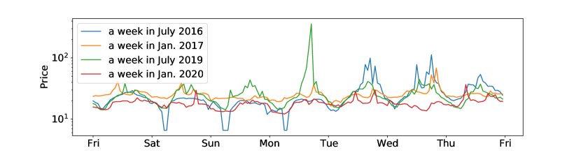
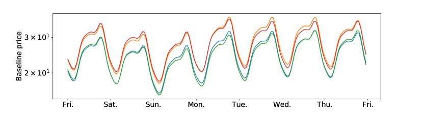
Figure 2: Price $p_{t}$ and baseline price $\exp\exp b_{t}$, over four different weeks, in July 2016, January 2017, July 2019, and January 2020.

Single forecast model.

Following the simple forecasting method from [45, §A], we fit an auto-regressive (AR) model to predict the residual $r_{t}=\log\log p_{t}-b_{t}$ over the next $23$ time periods, given the previous $24$. The residual AR model has the form

$$(\hat{r}_{t+1|t},\ldots,\hat{r}_{t+23|t})=\Gamma(r_{t-23},\ldots,r_{t}),$$

where $\Gamma\in{\mbox{\bf R}}^{23\times 24}$ is the AR parameter matrix. We fit $\Gamma$ using ridge regression on $43633$ training data points. Our final (single) price forecast is then given by

$$\hat{p}_{\tau|t}=\exp\exp\left(b_{\tau}+\Gamma_{\tau-t}(r_{t-23},\ldots,r_{t})\right),$$

where $\Gamma_{\tau-t}$ is the $(\tau-t)$th row of $\Gamma$. These forecasts have an RMS log-price error of $0.30$, a reduction from the baseline RMS log-price error $0.38$. This means our forecasts are typically off from the true price by around $35\%$. (If our forecasts were much better, then there would no need to use MF-MPC instead of MPC.)

The forecast error varies with $\tau-t$, the number of hours forward that we are predicting. The RMS log-price error versus $\tau-t$ is shown in figure 3. We can see that our prediction of the next hour’s price (i.e., $\tau-t=1$) is typically around $32\%$. For larger prediction horizons it increases. Our predictions 24 hours in the future (i.e., $\tau-t=23$) have RMS log-error $37\%$, still well below the RMS log-error of the baseline alone, which is $46\%$.

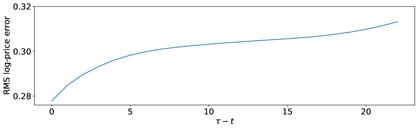
Figure 3: RMS forecast error for log-price versus $\tau-t$.

Multi-forecast model.

Denote the AR forecast error at $\tau$ given start time $t$ as

$$e_{\tau|t}=\log\log p_{\tau}-\log\log\hat{p}_{\tau|t}.$$

The statistics of these errors varies with the start time hour of the week, so we fit a different mean and a different covariance matrix for each hour of the week. The $24\times 7=168$ mean vectors denoted as $\mu_{m}$, $m=1,\ldots,168$, are empirical means. We fit $168$ covariance matrices to the errors, denoted $\Sigma_{m}$, $m=1,\ldots,168$, using a Laplacian regularized stratified model [70, 69]. Our graph on the stratified variable, in this case hour of the week, is a cycle graph with $24\times 7$ vertices. We use the solver implemented in [68] to fit the models.

Scenario sampling.

Given a start time $t$, $S$ samples $(e_{t+1|t}^{i},\ldots,e_{t+23|t}^{i})$, $i=1,\ldots,S$ are generated IID from $\mathcal{N}(\mu_{m},\Sigma_{m})$, where $m$ is the hour of the week for $t$. From these we obtain our price forecasts as

$$\hat{p}_{\tau|t}^{i}=\exp\exp\left(b_{\tau}+\Gamma_{\tau-t}(r_{t-23},\ldots,r_{t})+e_{\tau|t}^{i}\right),\quad\tau=t+1,\ldots,t+23,\quad i=1,\ldots,S.$$

Figure 4 shows the actual price, baseline, single forecast, and three random sample forecasts in the first 24 test hours.

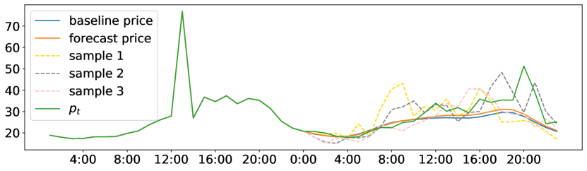
Figure 4: Baseline price, forecast price, and three price samples in the first 24 test hours, and the price data from the last 24th training hour to the first 24th test hour.

3.4 Simulation results

Policies.

We simulate a number of different policies over the 8 week period at the end of our data.

• MPC using the single forecast.

• MF-MPC with $S=20,40,80,160$, $320$, and $640$.

• IP-MPC, with minibatch size $b=20$, for a number of iterations $1,2,4,8,16,32$.

The MF-MPC policies (with different numbers of scenarios) and IP-MPC use the same samples in the same order, so with $1$ iteration, IP-MPC uses the same set of samples as MF-MPC with $S=20$ samples, and so on. For IP-MPC, we start at the MPC plan, so with zero iterations, this coincides with simple MPC. We use step sizes $\alpha_{k}=7/k$.

Prescient bound.

To get a performance bound, we compute the exact optimal charging with all future prices known. (This is a single LP that extends over the test period.) The resulting cost is $-62.3$ per hour, i.e., we make an averge profit of $\$62.30$ per hour. This is an upper bound on how well any policy can do.

Results.

We ran MF-MPC and IP-MPC for $10$ trials, with different sets of randomly generated scenarios, and we report the averaged result over the $10$ trials. The cost per hour for our policies is shown in figure 5. We can see that MF-MPC gives an improvement over MPC, with $S=640$ samples reducing cost from around $-38.8$ to around $-41.5$, around $2/3$ of the optimal average cost from our prescient bound. We can also see that MF-MPC with $S=640$ scenarios is not significantly better than $S=320$, and that $S=160$ gives us a reasonable fraction of the improvement over MPC.

The figure also shows that IP-MPC performs well. For $4$ iterations, IP-MPC uses the first $80$ samples and achieves a cost that is not far from MF-MPC $S=80$, despite $4$ iterations of IP-MPC giving only a very crude approximate solution of the associated MF-MPC problem. For $16$ iterations IP-MPC uses the first $320$ samples and achieves performance not too far from MF-MPC with $S=320$ samples. Running IP-MPC for even $32$ iterations does not solve the batch MF-MPC planning problem to high (or even modest) accuracy, but it yields a policy that does very well.

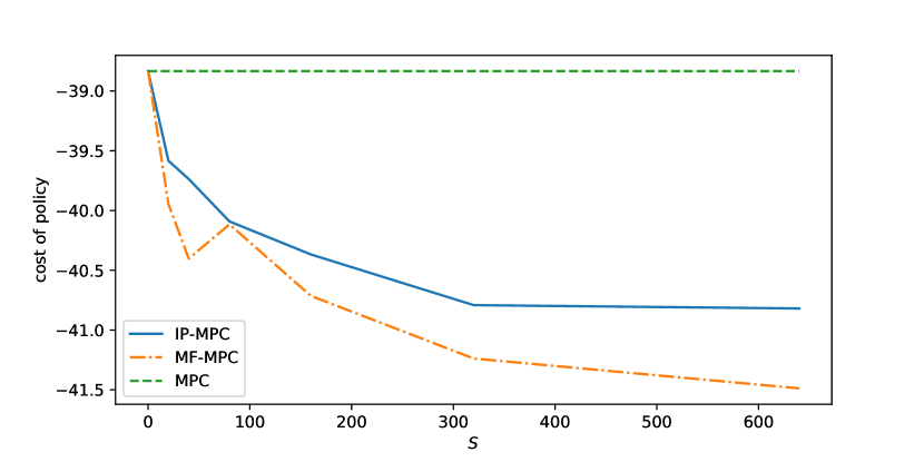
Figure 5: Cost per hour of various policies, including MPC, MF-MPC with different numbers of scenarios $S$, and IP-MPC for different numbers of iterations. The per hour cost of the prescient policy with all future prices known is $-62.3$.

Computation times.

We use CVXPY [18, 4] and the solver ECOS [20]. Simulating the MPC policy over 8 weeks (i.e., $1344$ hours) takes $33$ seconds, which means around $0.025$ seconds per policy evaluation. Simulating MF-MPC with 640 samples takes 2268 seconds, corresponding to $1.69$ seconds per policy evaluation. Using disciplined parameterized programming [3], running 32 IP-MPC iterations takes 1023 seconds, corresponding to $0.76$ seconds per policy evaluation.

4 Conclusion

IP-MPC is an iterative method for evaluating an MF-MPC policy, with each iteration involving the solution of a single forecast MPC problem. In the limit as the number of iterations increases, IP-MPC coincides with MF-MPC. More interesting to us, and evident in our example, is that IP-MPC can deliver much of the benefit of MF-MPC with a modest number of iterations, well before the IP-MPC policy is close to MF-MPC.

Our example suggests a reasonable general design approach. First, design a standard (single forecast) MPC control policy, choosing the objective and constraints, and tuning their parameters, to achieve good closed-loop performance, ideally on real data that was not used to develop the forecaster. Many variations on the objective and constraints can be tried out, since the policy is relatively fast to evaluate. Then, try out MF-MPC with varying numbers of scenarios to see what improvement (if any) is obtained over MPC, while possibly making small changes to the parameters to improve performance. Finally, try out IP-MPC, experimenting with the step length sequence and number of scenarios.

References

- [1] K. Abughalieh and S. Alawneh. A survey of parallel implementations for model predictive control. IEEE Access, 7:34348–34360, 2019.
- [2] A. Afram and F. Janabi-Sharifi. Theory and applications of HVAC control systems–a review of model predictive control (MPC). Building and Environment, 72:343–355, 2014.
- [3] A. Agrawal, B. Amos, S. Barratt, S. Boyd, S. Diamond, and J. Kolter. Differentiable convex optimization layers. In Advances in Neural Information Processing Systems, pages 9558–9570, 2019.
- [4] A. Agrawal, R. Verschueren, S. Diamond, and S. Boyd. A rewriting system for convex optimization problems. Journal of Control and Decision, 5(1):42–60, 2018.
- [5] S. Arpón, T. Homem-de Mello, and B. Pagnoncelli. An ADMM algorithm for two-stage stochastic programming problems. Annals of Operations Research, 286(1):559–582, 2020.
- [6] G. Banjac, B. Stellato, N. Moehle, P. Goulart, A. Bemporad, and S. Boyd. Embedded code generation using the OSQP solver. In 2017 IEEE 56th Annual Conference on Decision and Control (CDC), pages 1906–1911. IEEE, 2017.
- [7] A. Bemporad and M. Morari. Robust model predictive control: A survey. In Robustness in identification and control, pages 207–226. Springer, 1999.
- [8] D. Bertsekas. Incremental gradient, subgradient, and proximal methods for convex optimization: A survey. Optimization for Machine Learning, 2010(1-38):3, 2011.
- [9] D. Bertsekas. Incremental proximal methods for large scale convex optimization. Mathematical programming, 129(2):163–195, 2011.
- [10] J. Birge and F. Louveaux. A multicut algorithm for two-stage stochastic linear programs. European Journal of Operational Research, 34(3):384–392, 1988.
- [11] S. Boyd and L. Vandenberghe. Convex Optimization. Cambridge University Press, 2004.
- [12] R. Caflisch. Monte Carlo and quasi-Monte Carlo methods. Acta numerica, 7:1–49, 1998.
- [13] E. Camacho and C. Bordons. Model predictive control. Springer science & business media, 2013.
- [14] P. Campo and M. Morari. Robust model predictive control. In 1987 American control conference, pages 1021–1026. IEEE, 1987.
- [15] R. Carli, G. Cavone, N. Epicoco, P. Scarabaggio, and M. Dotoli. Model predictive control to mitigate the COVID-19 outbreak in a multi-region scenario. Annual Reviews in Control, 50:373–393, 2020.
- [16] C. Cutler and B. Ramaker. Dynamic matrix control: A computer control algorithm. In Joint Automatic Control Conference, volume 17, page 72, 1980.
- [17] W. de Oliveira. Risk-averse stochastic programming and distributionally robust optimization via operator splitting. Set-Valued and Variational Analysis, pages 1–31, 2021.
- [18] S. Diamond and S. Boyd. CVXPY: A Python-embedded modeling language for convex optimization. Journal of Machine Learning Research, 2016.
- [19] Y. Ding, L. Wang, Y. Li, and D. Li. Model predictive control and its application in agriculture: A review. Computers and Electronics in Agriculture, 151:104–117, 2018.
- [20] A. Domahidi, E. Chu, and S. Boyd. ECOS: An SOCP solver for embedded systems. In European Control Conference (ECC), pages 3071–3076, 2013.
- [21] J. Drgoňa, J. Arroyo, I. Figueroa, D. Blum, K. Arendt, D. Kim, E. Ollé, J. Oravec, M. Wetter, D. Vrabie, and L. Helsen. All you need to know about model predictive control for buildings. Annual Reviews in Control, 2020.
- [22] S. Engell. Online optimizing control: The link between plant economics and process control. In 10th International Symposium on Process Systems Engineering, volume 27, pages 79–86. Elsevier, 2009.
- [23] U. Eren, A. Prach, B. Koçer, S. Raković, E. Kayacan, and B. Açıkmeşe. Model predictive control in aerospace systems: Current state and opportunities. Journal of Guidance, Control, and Dynamics, 40(7):1541–1566, 2017.
- [24] J. Felez, Y. Kim, and F. Borrelli. A model predictive control approach for virtual coupling in railways. IEEE Transactions on Intelligent Transportation Systems, 20(7):2728–2739, 2019.
- [25] C. Garcia, D. Prett, and M. Morari. Model predictive control: Theory and practice—a survey. Automatica, 25(3):335–348, 1989.
- [26] P. Glynn and D. Iglehart. Importance sampling for stochastic simulations. Management science, 35(11):1367–1392, 1989.
- [27] B. Golub, M. Holmer, R. McKendall, L. Pohlman, and S. Zenios. A stochastic programming model for money management. European Journal of Operational Research, 85(2):282–296, 1995.
- [28] L. Grüne and J. Pannek. Nonlinear model predictive control, 2011.
- [29] T. Heirung, J. Paulson, J. O’Leary, and A. Mesbah. Stochastic model predictive control – how does it work? Computers & Chemical Engineering, 114:158–170, 2018.
- [30] K. Holkar and L. Waghmare. An overview of model predictive control. International Journal of Control and Automation, 3(4):47–63, 2010.
- [31] T. Hovgaard, S. Boyd, and J. Jørgensen. Model predictive control for wind power gradients. Wind Energy, 18(6):991–1006, 2015.
- [32] J. Hu, Y. Shan, J. Guerrero, A. Ioinovici, K. Chan, and J. Rodriguez. Model predictive control of microgrids – an overview. Renewable and Sustainable Energy Reviews, 136:110422, 2021.
- [33] M. Kochenderfer, T. Wheeler, and K. Wray. Algorithms for decision making. Mit Press, 2022.
- [34] N. Lazic, T. Lu, C. Boutilier, M. Ryu, E. J. Wong, B. Roy, and G. Imwalle. Data center cooling using model-predictive control. In Proceedings of the Thirty-second Conference on Neural Information Processing Systems (NeurIPS-18), pages 3818–3827, Montreal, QC, 2018.
- [35] J. Lee. Model predictive control: Review of the three decades of development. International Journal of Control, Automation and Systems, 9(3):415–424, 2011.
- [36] B. Lemaire. The proximal algorithm. International Series of Numerical Mathematics, pages 73 – 87, 1989.
- [37] J. Linderoth and S. Wright. Implementing decomposition algorithms for stochastic programming on a computational grid. Technical Report ANL/MCS-P909–0101, 2001.
- [38] S. Lucia, T. Finkler, D. Basak, and S. Engell. A new robust NMPC scheme and its application to a semi-batch reactor example. IFAC Proceedings Volumes, 45(15):69–74, 2012.
- [39] J. Maciejowski. Predictive control: with constraints. Pearson education, 2002.
- [40] M. Maiworm, T. Bäthge, and R. Findeisen. Scenario-based model predictive control: Recursive feasibility and stability. IFAC-PapersOnLine, 48(8):50–56, 2015.
- [41] J. Mattingley and S. Boyd. CVXGEN: A code generator for embedded convex optimization. Optimization and Engineering, 13(1):1–27, 2012.
- [42] D. Mayne. Model predictive control: Recent developments and future promise. Automatica, 50(12):2967–2986, 2014.
- [43] D. Mayne, M. Seron, and S. Raković. Robust model predictive control of constrained linear systems with bounded disturbances. Automatica, 41(2):219–224, 2005.
- [44] A. Mesbah. Stochastic model predictive control: An overview and perspectives for future research. IEEE Control Systems Magazine, 36(6):30–44, 2016.
- [45] N. Moehle, E. Busseti, S. Boyd, and M. Wytock. Dynamic energy management. In Large Scale Optimization in Supply Chains and Smart Manufacturing, pages 69–126. Springer, 2019.
- [46] M. Morari and J. Lee. Model predictive control: past, present and future. Computers & Chemical Engineering, 23(4-5):667–682, 1999.
- [47] D. Munoz de la Penad, A. Bemporad, and T. Alamo. Stochastic programming applied to model predictive control. In Proceedings of the 44th IEEE Conference on Decision and Control, pages 1361–1366. IEEE, 2005.
- [48] N. Parikh and S. Boyd. Proximal algorithms. Foundations and Trends in optimization, 1(3):127–239, 2014.
- [49] T. Péni, B. Csutak, G. Szederkényi, and G. Röst. Nonlinear model predictive control with logic constraints for COVID-19 management. Nonlinear Dynamics, 102(4):1965–1986, 2020.
- [50] PJM data miner 2. Available at http://dataminer2.pjm.com/list.
- [51] A. Prékopa. Two-stage stochastic programming problems. In Stochastic Programming, pages 373–423. Springer, 1995.
- [52] J. Primbs. Dynamic hedging of basket options under proportional transaction costs using receding horizon control. International Journal of Control, 82(10):1841–1855, 2009.
- [53] D. Raimondo, D. Limon, M. Lazar, L. Magni, and E. Camacho. Min-max model predictive control of nonlinear systems: A unifying overview on stability. European Journal of Control, 15(1):5–21, 2009.
- [54] S. Raković and W. Levine. Handbook of model predictive control. Springer, 2018.
- [55] J. Rawlings, D. Mayne, and M. Diehl. Model predictive control: Theory, computation, and design, volume 2. Nob Hill Publishing Madison, WI, 2017.
- [56] J. Richalet, A. Rault, J. L. Testud, and J. Papon. Model predictive heuristic control. Automatica (journal of IFAC), 14(5):413–428, 1978.
- [57] R. Rockafellar. Monotone operators and the proximal point algorithm. SIAM journal on control and optimization, 14(5):877–898, 1976.
- [58] R. Rockafellar. Progressive decoupling of linkages in optimization and variational inequalities with elicitable convexity or monotonicity. Set-Valued and Variational Analysis, 27(4):863–893, 2019.
- [59] R. Rockafellar and R. Wets. Scenarios and policy aggregation in optimization under uncertainty. Mathematics of operations research, 16(1):119–147, 1991.
- [60] A. Ruszczyński. A regularized decomposition method for minimizing a sum of polyhedral functions. Mathematical programming, 35(3):309–333, 1986.
- [61] A. Ruszczyński. Decomposition methods. Handbooks in operations research and management science, 10:141–211, 2003.
- [62] G. Sand and S. Engell. Modeling and solving real-time scheduling problems by stochastic integer programming. Computers & chemical engineering, 28(6-7):1087–1103, 2004.
- [63] S. Sen, R. Doverspike, and S. Cosares. Network planning with random demand. Telecommunication systems, 3(1):11–30, 1994.
- [64] S. Sen, J. Mai, and J. L. Higle. Solution of large scale stochastic programs with stochastic decomposition algorithms. In Large Scale Optimization, pages 388–410. Springer, 1994.
- [65] A. Shapiro. Monte Carlo sampling approach to stochastic programming. In ESAIM: Proceedings, volume 13, pages 65–73. EDP Sciences, 2003.
- [66] B. Stellato, G. Banjac, P. Goulart, A. Bemporad, and S. Boyd. OSQP: An operator splitting solver for quadratic programs. Mathematical Programming Computation, 12(4):637–672, 2020.
- [67] N. Topaloglou, H. Vladimirou, and S. Zenios. A dynamic stochastic programming model for international portfolio management. European Journal of Operational Research, 185(3):1501–1524, 2008.
- [68] J. Tuck, S. Barratt, and S. Boyd. A distributed method for fitting Laplacian regularized stratified models. Journal of Machine Learning Research, 22(60):1–37, 2021.
- [69] J. Tuck and S. Boyd. Eigen-stratified models. Optimization and Engineering, pages 1–23, 2021.
- [70] J. Tuck and S. Boyd. Fitting Laplacian regularized stratified Gaussian models. Optimization and Engineering, pages 1–21, 2021.
- [71] R. Van Slyke and R. Wets. L-shaped linear programs with applications to optimal control and stochastic programming. SIAM journal on applied mathematics, 17(4):638–663, 1969.
- [72] Y. Wang and S. Boyd. Fast model predictive control using online optimization. IEEE Transactions on control systems technology, 18(2):267–278, 2009.
- [73] Y. Xi, D. Li, and S. Lin. Model predictive control—status and challenges. Acta Automatica Sinica, 39(3):222–236, 2013.
- [74] S. Zenios, M. Holmer, R. McKendall, and C. Vassiadou-Zeniou. Dynamic models for fixed-income portfolio management under uncertainty. Journal of Economic Dynamics and Control, 22(10):1517–1541, 1998.