Quantum fluctuations, particles and entanglement:
a discussion towards the solution of
the quantum measurement problems

Abstract

The quantum measurement problems are revisited from a new perspective.

One of the main ideas of this work is that the basic entities of our world are various types of particles, elementary or composite. It follows that each elementary process, hence each measurement process at its core, is a spacetime, pointlike, event. Another key idea is that, when a microsystem $\psi$ gets into contact with the experimental device, factorization of $\psi$ rapidly fails and entangled mixed states appear. The wave functions for the microsystem-apparatus coupled systems for different measurement outcomes then lack overlapping spacetime support. It means that the aftermath of each measurement is a single term in the sum: a “wave-function collapse”.

Our discussion leading to a diagonal density matrix, $\rho={\rm diag}(|c_{1}|^{2},\ldots,|c_{n}|^{2},\ldots)$ shows how the information encoded in the wave function $|\psi\rangle=\sum_{n}c_{n}|n\rangle$ gets transcribed, via entanglement with the experimental device and environment, into the relative frequencies ${\cal P}_{n}=|c_{n}|^{2}$ for various experimental results $F=f_{n}$.

These results represent new, significant steps towards filling in the logical gaps in the standard interpretation based on Born’s rule, and replacing it with a more natural one. Accepting objective reality of quantum fluctuations, independent of any experiments, and independently of human presence, one renounces the idea that in a fundamental, complete theory of Nature the result of each single experiment must necessarily be predictable.

A few well-known puzzles such as the Schrödinger cat conundrum and the EPR paradox are briefly reviewed: they can all be naturally explained away.

1 Introduction

The so-called “quantum measurement problem” has been with us ever since the establishment of quantum mechanics in the first quarter of the last century. The validity of quantum mechanics has since passed every tests made, first through an impressive success in atomic physics. Today, we may note that the standard $SU(3)_{QCD}\times(SU(2)\times U(1))_{GW\!S}$ model of the fundamental (strong and electroweak) interactions, based on the relativistic quantum mechanics of the particles and fields, is one of the most successful and precisely tested physics theories known so far. We should mention also many beautiful quantum mechanical phenomena in condensed matter physics, such as superfluidity, superconductivity, quantum Hall effect, Bose-Einstein condensation of ultracold atoms, and so on.

In spite of all this, the probabilistic nature of the quantum mechanical predictions has always kept us with an uneasy feeling, that something fundamental is missing in our understanding of quantum mechanics.

Such a feeling is often expressed in the form of a “quantum measurement problem”. It actually represents several different issues. Is the wave-function-collapse which apparently occurs at the moment of a measurement real? Is the macroscopic superposition of the states involving the microsystem, the experimental apparatus, and eventually the environment (and in principle the rest of the world), relevant? Are we living in a section of the forever branching many-worlds tree? Or does the whole world spontaneously collapse (or localize) from time to time? Or is the wave function just an (extremely clever) bookkeeping device which is nothing truly physical but that somehow encodes the information relating past experimental results to future ones? Together with these philosophical “problems”, there is a conceptual conflict between the smooth and deterministic time evolution of the systems described by the Schrödinger equation, and the quantum jumps occurring regularly in atoms, nuclei and molecules, or at the moments of the measurements. And above all, is Born’s rule something which follows in principle from the Schrödinger equation involving everything from the microsystem, the measuring apparatus, and the whole world, via some mysterious effectively nonlinear evolution? And independently of all this, is it conceivable that a complete, fundamental theory of Nature should not be able to predict the result of each single experiment uniquely?

This work addresses all of these questions and puzzles. The careful reader will find a clear answer or resolution to each of them, in the following discussions. Our answer to the last question is throughout the work: it is summarized in the Abstract and in Sec. 10.

The actual measurement devices can vastly differ in their nature, size, materials used, and technologies employed, from a simple photographic plate, cloud and bubble chambers filled with liquid or vapour, spark chambers and MWPC made with metal plates, wires and gas, the neutrino detectors made of a huge tank of pure water and tens of thousands of photomultipliers, to the state-of-the-art silicon detectors and some future apparatus which uses superconducting materials for dark matter search. Such an enormous diversity of the experimental devices requires that an equally vast simplification be made, to capture the essence of quantum measurements.

We know that, independent of the details, a good experimental device faithfully reflects the quantum fluctuations of the system being studied, described by the wave function $\psi$. Indeed, the result of each single experiment is, in general, apparently random and unpredictable . Yet, the information contained in the wave function $\psi$, encoded as the expectation values for any variable $F$ (and all functions thereof)

$${\bar{F}}\equiv\langle\psi|F|\psi\rangle\;,$$ (1.1)

fully manifests itself, as a (frequency-) average of the experimental outcomes, ${\bar{f_{n}}}$,

$${\bar{f_{n}}}=\sum_{n}f_{n}\,{\cal P}_{n}\;,\qquad{\cal P}_{n}=|\langle n|\psi\rangle|^{2}\;,$$ (1.2)

where $F|n\rangle=f_{n}|n\rangle$, and ${\cal P}_{n}$ is the relative frequency for $f_{n}$. Such a prediction of quantum mechanics is verified by countless experiments.

The prediction (1.2) would follow, if one assumes that the probability of each single measurement of $F$ in the state $\psi$ to give $f_{n}$, is given by $P_{n}=|\langle n|\psi\rangle|^{2}\;,$ i.e., Born’s rule. This assumption is presented in most textbooks as one of the fundamental postulates of quantum mechanics .

We introduce here a slight change of perspective. The fundamental laws of quantum mechanics are represented by the expectation values (quantum fluctuation average) of all variables in the system. Such quantum fluctuations are there, independently of any experiments. As will be illustrated and discussed in Sec. 2, Sec. 5 and Sec. 10, the new point of view constitutes a small but nonetheless significant conceptual departure from the traditional way of interpreting the fundamental laws of quantum mechanics.

The main results of this work (Sec. 5.6) follow from the following two key ideas. The first ([A] below) which leads to the resolution of most of the puzzles and paradoxes associated with the measurement processes, comes from the observation that the basic building blocks of our world are various types of particles. The elementary constituents of Nature (the electron, the muon, the photon, the quarks, the $W,Z$ bosons, the gluons, etc.) are all pointlike objects (particles), and all the fundamental interactions occur at definite spacetime points, the vertices of the Feynman diagrams.

It follows that [A] at its heart each experiment is a space-time pointlike event, or, triggered by one . Such an observation was at the core of Einstein’s explanation of the photoelectric effects based on Planck’s light quantum.

One might object that certain static or adiabatic effects such as the Coulomb potential describing the atomic structures, the magnetic fields used in the Stern-Gerlach experiment or in a momentum measurement, and the electric and magnetic fields used to accelerate particles in high-energy experiments, do not represent themselves spacetime pointlike events. These are particular effects of quantum electrodynamics, the quantum theory of particles (i.e., electrons and photons). Nevertheless, these effects do not inject energy to the microscopic system in interaction with them, suddenly enough to trigger the chain ionization processes, hadronic cascades, and the amplification and the consequent recording of the particle fingerprints by the device, characteristic of a measurement process. This fact allows us to use these static or adiabatic effects in many useful ways, while at the same time keeping them from becoming a measurement themselves. This discussion hopefully clarifies, partially at least, the question which often arises: which part of the processes should be regarded as “the measurement” and which part not (e.g. a preparation) .

We also note that the molecules, atoms, nuclei, and even particles such as proton, neutron and pions (which were once considered as elementary particles) are all bound states (i.e., composite particles) made of some other, underlying constituents. This fact does not affect the statement of the preceding paragraphs: all these composite objects behave perfectly as pointlike particles at appropriate distance scales, much larger than their characteristic sizes.

Taking into account this eventlike nature of the measurement processes will indeed be central in showing the absence of interferences among the distinct states of the microscopic quantum and macroscopic apparatus combined system, which is one of the principal issues in the “quantum measurement problems”. See the discussions in Sec. 5 $\sim$ Sec. 8 below.

A second main input of this work ([B] below) concerns the central role played by factorization and entanglement (see Sec. 4) in the measurement processes. The concept of pure state, e.g., of the wave function $|\psi\rangle$ describing the microsystem before the measurement, is a (usually very) good approximation, if the experiment is carefully prepared. Still, it describes a subsystem of a larger system containing the experimental apparatus and the rest of the world. Exact factorization means that the wave function of the whole system before the measurement has a factorized form

$$|\Psi\rangle=|\psi\rangle\otimes|\Phi;Env\rangle\;$$ (1.3)

(see Sec. 5 for the definition of the apparatus-environment coupled state, $|\Phi;Env\rangle$). The second key idea of this work [B] is that, during the measurement process, factorization of $|\psi\rangle$, as in (1.3), rapidly fails as a result of interactions between it and the measurement device and with the rest of the world, and as a result an entangled mixed state labelled by the unique measurement reading emerges, see (5.7), (5.19) below. The result is a state-vector reduction, often called a “wave-function collapse” .

The main result of this work (summarized in Sec. 5.6) which follows from the analyses of Sec. 2 $\sim$ Sec. 5, is the well-known quantum mechanical prediction, that measurements done on the state $\psi$

$$|\psi\rangle=\sum_{n}c_{n}\,|n\rangle\;,\qquad F|n\rangle=f_{n}|n\rangle\;,$$ (1.4)

give various results $F=f_{n}$, with relative frequencies ${\cal P}_{n}=|c_{n}|^{2}$. This may sound almost identical to the standard postulate of quantum mechanics: “a measurement done on the state $\psi$ will give various results $F=f_{n}$, with probabilities, $P_{n}=|c_{n}|^{2}$” (Born’s rule).

What is missing in Born’s rule, however, is the explanation of how the information about the quantum fluctuations encoded in the wave function $\psi$ gets transcribed, through the measurement process, into the expected relative frequencies of finding various results $F=f_{n}$, ${\cal P}_{n}=|c_{n}|^{2}$, and the understanding of why and how the state-vector reduction takes place, after each experiment.

The contribution of this work is to indicate the first steps to fill in these gaps.

In Sec. 6 $\sim$ Sec. 8 we discuss several well-known puzzles and apparent paradoxes, and show how they are all naturally explained. Sec. 9 discusses a few general ideas about the universe and the quantum measurements, which come out of our considerations. We summarize and conclude in Sec. 10.

2 The expectation values versus Born’s rule

We first review the equivalence of the information contained in the expectation values (the quantum fluctuation averages) and Born’s rule.

2.1 The angular momentum and spin

In an angular momentum-spin system, the quantum fluctuations are famously expressed by the fact that in a state of definite angular momentum magnitude ${\mathbbm{J}}^{2}=j(j+1)$, each component of ${\mathbbm{J}}$ can attain only up to the maximum absolute value $j$, which is smaller (for $j\neq 0$) than the square root of ${\mathbbm{J}}^{2}$. This is due to the fact that the three components $J_{x},J_{y},J_{z}$ do not commute with each other: they are not mutually compatible . In a state with definite $({\mathbbm{J}}^{2},J_{z})$, the values of $J_{x}$ and $J_{y}$ are undetermined - Heisenberg’s uncertainties. Quantitatively, in the state (we set $\hbar=1$)

$${\mathbbm{J}}^{2}|j,m\rangle=j(j+1)|j,m\rangle\;;\quad J_{z}|j,m\rangle=m|j,m\rangle\;,\qquad m=j,j-1,\ldots,-j\;,$$ (2.1)

the values of $J_{x}$ and $J_{y}$ are fluctuating, such that their quantum average satisfies:

$$\langle j,m|J_{x}^{2}+J_{y}^{2}|j,m\rangle=\langle j,m|{\mathbbm{J}}^{2}-J_{z}^{2}|j,m\rangle=j(j+1)-m^{2}\;.$$ (2.2)

Each experiment measuring $J_{x}$, for instance, observes one of the possible values, $J_{x}=j,j-1,\ldots,-j$, in accordance with (2.2).

Let us check these predictions against Born’s rule. Though this discussion contains nothing really new, it may still be refreshing to see the well-known results from a slightly unconventional perspective.

2.1.1 Spin $\tfrac{1}{2}$

In the state of spin up, i.e., $s_{z}=+\tfrac{1}{2}$,

$$|\!\uparrow\rangle=|\tfrac{1}{2},\tfrac{1}{2}\rangle\;,$$ (2.3)

the measurement of $s_{x}$ will give $\pm\tfrac{1}{2}$, with no preference for $\pm$ on the average, and also with ${\bar{s_{x}^{2}}}\sim{\bar{s_{y}^{2}}}$, so we find from (2.2),

$$\langle\tfrac{1}{2},\tfrac{1}{2}|s_{x}^{2}|\tfrac{1}{2},\tfrac{1}{2}\rangle=\frac{1}{4}\;.$$ (2.4)

Each experiment will thus give the result $s_{x}=\pm\frac{1}{2},$ with equal relative frequencies

$${\cal P}_{+}={\cal P}_{-}=\frac{1}{2}\;,$$ (2.5)

in accordance with Born’s rule ($|\pm\rangle$ are the eigenstates of $s_{x}$):

$$P_{+}=|\langle+|\uparrow\rangle|^{2}=\frac{1}{2}\;;\qquad P_{+}=|\langle-|\uparrow\rangle|^{2}=\frac{1}{2}\;.$$ (2.6)

Consider instead a measurement of the spin component $s_{n}$ in the generic direction

$$s_{n}\equiv{\mathbf{s}}\cdot{\mathbf{n}}\;,\qquad{\bf n}=(\sin\theta\cos\phi,\sin\theta\sin\phi,\cos\theta)\;,$$ (2.7)

in the state $|\!\!\uparrow\rangle$. By rotating the space axes this problem can be refrased as that of measuring $s_{z}$ in the state,

$$|n\rangle=c_{1}|\uparrow\rangle+c_{2}|\downarrow\rangle=\left(\begin{array}[]{c}e^{-i\phi/2}\cos\tfrac{\theta}{2}\\ e^{i\phi/2}\sin\tfrac{\theta}{2}\end{array}\right)\;,\qquad s_{n}|n\rangle=\frac{1}{2}|n\rangle\;,$$ (2.8)

i.e., the state in which the spin is directed towards the unit vector ${\bf n}$. The quantum fluctuation of $s_{z}$ is expressed in the formulae,

$$\langle n|s_{z}|n\rangle=\frac{1}{2}(|c_{1}|^{2}-|c_{2}|^{2})\;,\qquad\langle n|s_{z}^{2}|n\rangle=\frac{1}{4}(|c_{1}|^{2}+|c_{2}|^{2})=\frac{1}{4}\;.$$ (2.9)

Note that this time the quantum fluctuations of $s_{z}$ towards $\frac{1}{2}$ and $-\frac{1}{2}$ are not equally likely, as the spin is directed in a generic direction ${\bf n}$. One finds from the above,

$$\frac{1}{2}({\cal P}_{\uparrow}-{\cal P}_{\downarrow})=\frac{1}{2}(|c_{1}|^{2}-|c_{2}|^{2})\;,\qquad\frac{1}{4}({\cal P}_{\uparrow}+{\cal P}_{\downarrow})=\frac{1}{4}\;,$$ (2.10)

hence

$${\cal P}_{\uparrow}=|c_{1}|^{2}=\cos^{2}\tfrac{\theta}{2}\;,\qquad{\cal P}_{\downarrow}=|c_{2}|^{2}=\sin^{2}\tfrac{\theta}{2}\\ \;.$$ (2.11)

This agrees with Born’s rule,

$$P_{\uparrow}=|\langle\uparrow|n\rangle|^{2}=|c_{1}|^{2}\;,\qquad P_{\downarrow}=|\langle\downarrow|n\rangle|^{2}=|c_{2}|^{2}\;.$$ (2.12)

2.1.2 Spin $\frac{3}{2}$

Measurement results of $J_{x}$ in the state $|J,J_{z}\rangle=|\tfrac{3}{2},\tfrac{3}{2}\rangle$ are dictated by the fluctuation formula (2.2),

$$\langle\tfrac{3}{2},\tfrac{3}{2}|J_{x}^{2}+J_{y}^{2}|\tfrac{3}{2},\tfrac{3}{2}\rangle=\frac{15}{4}-\frac{9}{4}=\frac{3}{2}\;.$$ (2.13)

This, together with the assumption that the fluctuations in the $x$ and $y$ directions are equal on the average, and also that fluctuations towards $J_{x}>0$ and $J_{x}<0$ are equally likely, yields

$$\frac{9}{4}{\cal P}(\tfrac{3}{2})+\frac{1}{4}{\cal P}(\tfrac{1}{2})=\frac{3}{8}\;.$$ (2.14)

Actually we have more information on the quantum fluctuations: we may use for instance

$$\langle\tfrac{3}{2},\tfrac{3}{2}|J_{x}^{4}|\tfrac{3}{2},\tfrac{3}{2}\rangle=\frac{21}{16}\;,$$ (2.15)

which gives

$$\frac{81}{16}{\cal P}(\tfrac{3}{2})+\frac{1}{16}{\cal P}(\tfrac{1}{2})=\frac{21}{32}\;.$$ (2.16)

Solving the system (2.14), (2.16) we find

$${\cal P}(\tfrac{3}{2})=\frac{1}{8}\;;\qquad{\cal P}(\tfrac{1}{2})=\frac{3}{8}\;.$$ (2.17)

On the other hand, Born’s rule gives directly

$$P(\tfrac{3}{2})=|\langle J_{x}=\tfrac{3}{2}|\tfrac{3}{2},\tfrac{3}{2}\rangle|^{2}=|\tfrac{1}{2\sqrt{2}}(1,\sqrt{3},\sqrt{3},1)\cdot\left(\begin{array}[]{c}1\\ 0\\ 0\\ 0\end{array}\right)|^{2}=\frac{1}{8}\;;$$ (2.18)

$$P(\tfrac{1}{2})=|\langle J_{x}=\tfrac{1}{2}|\tfrac{3}{2},\tfrac{3}{2}\rangle|^{2}=|\tfrac{\sqrt{3}}{2\sqrt{2}}(-1,\frac{1}{\sqrt{3}},\frac{1}{\sqrt{3}},1)\cdot\left(\begin{array}[]{c}1\\ 0\\ 0\\ 0\end{array}\right)|^{2}=\frac{3}{8}\;,$$ (2.19)

in agreement with (2.17). A similar check can be made readily for the initial state, $|\tfrac{3}{2},\tfrac{1}{2}\rangle$.

2.2 General variables

The wave function is given by $|\psi\rangle$, and let us assume that one is now measuring a dynamical variable $F$. We assume that $|\psi\rangle$ has the form

$$|\psi\rangle=\sum_{n}c_{n}|n\rangle\;,\qquad{F}|n\rangle=f_{n}|n\rangle\;,\qquad\sum_{n}|c_{n}|^{2}=1\;,$$ (2.20)

where $|n\rangle$’s are the eigenstates of the associated self-adjoint operator ${F}$. For simplicity, the eigenvalues $f_{n}$ are assumed to be non degenerate .

In the state $|\psi\rangle$ the values of $F$ are fluctuating, among all possible $f_{n}$’s. The measurement device each time picks up one of them, $F=f_{m}$, apparently randomly. However the frequency-averaged experimental result

$${\bar{f_{n}}}=\sum_{n}{\cal P}_{n}f_{n}\;,$$ (2.21)

where ${\cal P}_{n}$ is the expected relative frequency for finding $F=f_{n}$, is equal, by assumption, to the quantum fluctuation average (the expectation value),

$${\bar{F}}=\langle\psi|{F}|\psi\rangle=\sum_{n}|c_{n}|^{2}f_{n}\;.$$ (2.22)

Now, identification of (2.21) with (2.22) would be valid if

$${\cal P}_{n}=|c_{n}|^{2}=|\langle n|\psi\rangle|^{2}\;,$$ (2.23)

which, in turn, would follow from Born’s probabilistic rule for each single experiment,

$$P_{n}=\langle\psi|\Pi_{n}|\psi\rangle=|c_{n}|^{2}\;,\qquad\Pi_{n}=|n\rangle\langle n|\;.$$ (2.24)

In other words, Born’s rule (2.24) is a sufficient condition for (2.21) $\sim$ (2.23) to hold, but it might in general not be necessary.

In order to show that it is also necessary, we must take into account more information about the fluctuation of the variable $F$,

$${\bar{O}}\equiv\langle\psi|O|\psi\rangle=\sum_{n}(f_{n})^{N}|c_{n}|^{2}\;,\qquad O=F^{N},\qquad N=1,2,\ldots\;,$$ (2.25)

and identifying them with

$${\overline{(f_{n})^{N}}}=\sum_{n}(f_{n})^{N}{\cal P}_{n}\;,\qquad N=1,2,\ldots\;.$$ (2.26)

The equivalence of Born’s rule and the fluctuation averages has been illustrated concretely in simple spin systems in the previous section.

In general, if the eigenvalues $f_{n}$ are nondegenerate, and if the Hilbert space is finite-dimensional (with dimension $D$), the expectation values (2.25) for $O=F,F^{2},\ldots,F^{D}$ are necessary, and sufficient, to yield Born’s rule (2.23). A simple proof which makes use of the nonvanishing Vandermonde determinant is given in Appendix A.

Actually, a more straightforward way to see the equivalence between ${\cal P}_{n}$ and $P_{n}$, is to consider, instead of various powers of $F$, a particular function of the variable $F$, which takes the value $1$ if $F=f_{n}$, and $0$ if $F\neq f_{n}$. One may construct a Kronecker-delta like operator in terms of the self-adjoint operator $F$,

$$\lim_{T\to\infty}\frac{1}{2T}\int_{-T}^{T}d\alpha\,e^{i\alpha(F-f_{n})}\;,$$ (2.27)

but it can be seen to be equivalent to the projection operator, $\Pi_{n}=|n\rangle\langle n|$. Its expectation value, the expected relative frequency ${\cal P}_{n}\times 1={\cal P}_{n}$, is indeed equal to

$$\langle\psi|\Pi_{n}|\psi\rangle=|\langle n|\psi\rangle|^{2}=|c_{n}|^{2}\;,$$ (2.28)

but this agrees with Born’s rule.

The discussion can be straightforwardly generalized to the position measurement, and to other measurements of any variable with continuous spectrum. In the case of a position measurement, $x$, the most straightforward way to see the equivalence is to consider a particular function of $x$, with small $\epsilon>0$,

$$f_{x_{0}}(x)=\begin{cases}\frac{1}{\epsilon}\;,&x\in\{x_{0},x_{0}+\epsilon\}\;;\\ 0\;,&\text{otherwise}\;.\end{cases}$$ (2.29)

Its expectation value

$$\langle\psi|f_{x_{0}}|\psi\rangle=\int dx\,f_{x_{0}}(x)\,|\psi(x)|^{2}\simeq|\psi(x_{0})|^{2}\;,$$ (2.30)

identified with (${\cal P}(x)$ being the expected relative frequency density)

$${\bar{f}}=\int dx\,f_{x_{0}}(x)\,{\cal P}(x)\simeq{\cal P}(x_{0})\;,$$ (2.31)

leads to (in the limit $\epsilon\to 0$)

$${\cal P}(x)\,dx=|\psi(x)|^{2}\,dx\;.$$ (2.32)

2.3 Summary

The assumption that the expectation value of a general function $O(F)$ of an operator $F$

$${\overline{O(F)}}=\langle\psi|O(F)|\psi\rangle=\sum_{n}|c_{n}|^{2}O(f_{n})\;$$ (2.33)

is to be interpreted as the prediction for the experimental average,

$${\overline{O({f_{n}}}})=\sum_{n}{\cal P}_{n}\,O(f_{n})\;,$$ (2.34)

where ${\cal P}_{n}$ is the (normalized) relative frequencies for finding $F=f_{n}$, leads to ${\cal P}_{n}=|\langle n|\psi\rangle|^{2}=|c_{n}|^{2}\;.$

3 Pure and mixed states

A system described by a wave function, (2.20)

$$|\psi\rangle=\sum_{n}c_{n}|n\rangle\,,\qquad F|n\rangle=f_{n}|n\rangle\;,$$ (3.1)

which contains in it the complete information on the state, is known as a pure state. A pure quantum state contains an enormous amount of information. Even a simple spin $\tfrac{1}{2}$ state (2.8), a “qubit”, can carry a big quantity of information covering the space, $CP^{1}\sim S^{2}$, to be contrasted with a classical bit, $(1\,\,{\rm or}\,\,0)$. We shall use below terms such as state, (true) quantum state, genuine quantum state, and pure state, interchangeably .

If for whatever reason such a complete information is lacking, we have a so-called mixed state, or a mixture. A mixed state is described by a density matrix instead of a wave function. Its definition, the general properties and the way it is used, are well known: they can be found in most textbooks (e.g., Chap. 7 of [1]).

Here let us just remember a few formulas. If the lack of information is due to the fact that the system $A$ observed (and the variables $F$ studied) is (refer to) a subsystem of the total system $\Sigma$, $A\subset\Sigma$, the wave function of $\Sigma$ may be written as

$$|\Psi\rangle=\sum_{n,\alpha}c_{n,\alpha}|n\rangle|\alpha\rangle\,,\qquad\sum_{n,\alpha}|c_{n,\alpha}|^{2}=1\;,$$ (3.2)

where $\{|n\rangle\}$ is an arbitrary orthonormal set of states (for instance, the eigenstates of the operator $F$ in (3.1)) describing the subsystem $A$, and ${\alpha}$ refer to all variables in $\Sigma/A$. The fluctuation average of a generic variable $G$ (pertinent to the subsystem $A$) is encoded in the expectation value,

$${\bar{G}}=\langle\Psi|G|\Psi\rangle=\mathop{Tr}\nolimits{\mathbbm{G}}\rho\;,\qquad({\mathbbm{G}})_{mn}\equiv\langle m|G|n\rangle\;,$$ (3.3)

where the density matrix is given by

$$(\rho)_{nm}\equiv\sum_{\alpha}c_{n,\alpha}\,c_{m,\alpha}^{*}\;.$$ (3.4)

The particular form of the density matrix (3.4) refers to the case of a subsystem $A\subset\Sigma$. The trace formula for ${\bar{G}}$ in (3.3), instead, is valid for a general mixed state.

As said already, a mixed state can arise for any other reason which causes the loss of the complete knowledge on the system. A well-known example of mixed state is a partially polarized light (i.e., a beam of photons whose polarization states are only statistically partially known). Another important mechanism for the emergence of a mixed state, relevant to our discussion of the measurement processes below, is that the measurements, which are spacetime, pointlike events (our key observation [A]), lead to the loss of the phase coherence among different terms. See (5.21) and (5.19) below.

The trace formula (3.3) generalizes the expression (2.22) for the fluctuation average in a pure state to the case of a mixed state.

4 Factorization vis-à-vis entanglement

An issue which has some formal similarity to the discussions in Sec. 5 below, and is in fact closely related to them, is factorization, which works with a remarkable precision under certain circumstances, actually making quantum mechanics a sensible physics theory at all. In simplest imaginable terms, the question is (symbolically) this: how could we study the physics of a single hydrogen atom, in spite of the fact that the wave function must be antisymmetrized with respect to exchanges of all electrons in the universe, according to the Fermi-Dirac statistics for identical fermions?

The answer is that, for instance for the two electrons, one in the laboratory, the other on the sun, the wave function is given by

$$\Psi=\frac{1}{\sqrt{2}}\left(\psi_{lab}({\mathbf{r}}_{1})\psi_{sun}({\mathbf{r}}_{2})-\psi_{lab}({\mathbf{r}}_{2})\psi_{sun}({\mathbf{r}}_{1})\right)\;,$$ (4.1)

but the second term is utterly negligible when

$${\mathbf{r}}_{1}\in{\rm Lab.}\;,\qquad{\mathbf{r}}_{2}\in{\rm Sun}\;,$$ (4.2)

as the wave function $\psi_{lab}$ (vis-à-vis, $\psi_{sun}$) has (spatial) support in a small region in the laboratory (in the sun). There is no overlap. Only the first term in (4.1) survives, and the laboratory electron is simply described by the wave function $\psi_{lab}({\mathbf{r}}_{1})$.

Instead of this symbolic example, one may consider the second hydrogen atom in the next room in the laboratory, e.g., two meters away. From Bohr’s radius for the hydrogen atom, one finds a suppression of the order of $10^{-18}$ for factorization failure. This rule-of-thumb estimate may give some idea about the exactness of our assertion in Sec. 5, even though there the question will be the lack of the overlap in spacetime supports.

Just to close a loophole in the discussion, we note that if the antisymmetrization is done with respect to the spin state, and not with respect to the space positions as in (4.1), the wave function does not factorize (the two electrons are entangled). In that case, we have an unknown mixture for the spin state of the laboratory electron.

In fact, factorization and entanglement are two faces of the same medal, both characterizing quantum mechanics universally. Certain aspects of quantum entanglement such as those briefly reviewed and discussed below in Sec. 8 in connection with the EPR paradox, have become one of the most ardently discussed topics of quantum mechanics, presumably because of some fascinating features involved (e.g., quantum nonlocality).

Actually, the occurrence of entanglement is much more general and indeed, ubiquitous. It does not depend on the Fermi-Dirac or Bose-Einstein statistics either, contrarily to what the above example might have erroneously suggested. All systems which have interacted with each other in the past are generally entangled. Any quantum system in which factorization does not hold in good approximation, is entangled and is, typically, in a mixed state. Our whole world is a large quantum system, in a complex, entangled mixed state. Macroscopic bodies in it generally exhibit classical behaviors because of entanglement with their environment [8, 9].

It is the factorized quantum states - those described by the wave function, e.g., of an atom or of an electron - that are truly extraordinary, and exceptional. The concept of a pure state $|\psi\rangle$ depends on the factorization of the system described by $\psi$, from the rest of the world. These states are carefully prepared by the experimentalist, inside many small isolated bubbles in the world (i.e., physics laboratories), by using sophisticated vacuum and clean-room technologies. Pure states (free particles) occur also in Nature, as a result of radioactivity on Earth, or as cosmic rays in interstellar space, for instance. See Sec. 9 for more discussions.

As will be seen below, factorization of $|\psi\rangle$ describing the microsystem which is the object of the measurement gets rapidly ruined during the measurement process as a result of the interactions between it and the measurement device as well as with the rest of the world, and a particular set of entangled mixed states labelled by the measurement readings emerge. The result is the “wave-function collapse”, or better, what may be perceived as such, see the discussions below.

5 Measurement processes

To have a complete picture of the measurement processes it is often assumed that the full wave function contains the microscopic state $|\psi\rangle$, the apparatus state $|\Phi\rangle$, and the state of the environment, $|Env\rangle$, the last containing everything outside the experimental device, such as the air molecules, the computer screen, the experimentalists, etc. The measurement process, on the state

$$|\psi\rangle=\sum_{n}c_{n}|n\rangle\,,\qquad F|n\rangle=f_{n}|n\rangle\;,$$ (5.1)

is supposed to proceed as (the states with index $0$ stand for the neutral state, before the reading of the results):

$$|\psi\rangle\otimes|\Phi_{0}\rangle\otimes|Env_{0}\rangle = \left(\sum_{n}c_{n}|n\rangle\right)\otimes|\Phi_{0}\rangle\otimes|Env_{0}\rangle$$ (5.2)

$$\longrightarrow \left(\sum_{n}c_{n}|n\rangle\otimes|\Phi_{n}\rangle\right)\otimes|Env_{0}\rangle$$ (5.3)

$$\longrightarrow \sum_{n}c_{n}|n\rangle\otimes|\Phi_{n}\rangle\otimes|Env_{n}\rangle\;,$$ (5.4)

where in the first step (5.3) the experimental device has read the measurement results, $f_{n}$, and in the final step (5.4) the environment has come to be aware of such a result (the experimentalist has seen the result on her/his computer screen).

This kind of formulas, apparently describing coherent superpositions of distinct macroscopic states, has given rise to innumerable debates in the literature as, most famously, in the so-called Schrödinger cat conundrum. Actually, the Schrödinger’s cat discussion involves several extra issues which are not present in the general measurement processes considered here. To avoid unnecessary complications and unavoidable confusion, we will postpone its discussion to Sec. 7.

Actually, the factorized form of the state vectors in (5.2) $\sim$ (5.4) (various $\otimes$ symbols), found often in the literature, is not valid in general, except for the first. The factorized form of the wave function of the microsystem $|\psi\rangle$ before the measurement, in the first line, (5.2), is correct by definition: we are assuming to have a microsystem described by $|\psi\rangle$ before the measurement.

The role of the environment or the entire world outside the measurement device, $|Env\rangle$, in measurement processes, is subtle. The factorized form $|\Phi\rangle\otimes|Env\rangle$ is not in general guaranteed, even before the actual experiment, i.e., even in (5.2). It suffices to consider the air molecules around, the casing of the device itself, etc., which all represent complicated entanglement between $|\Phi\rangle$ and $|Env\rangle$. This means also that the boundary (or distinction) between what is to be considered as the experimental device and what belongs to the rest, is not well defined. More precisely, the exact boundary between the two is largely arbitrary, and must be regarded as conventional.

Also, the experimental device, after the reading of the measurement, is in a classical state. This fact, the emergency of the classical behavior of the experimental apparatus, is believed to be due to the entanglement [8, 9] between $|\Phi\rangle$ and $|Env\rangle$.

In spite of all this, every experimentalist knows perfectly well which part of her (or his) device is essential, and that the blurred boundary between it and the environment does not affect her (his) results, to any significant degree. She (or he) would not worry where the exact boundary between the measurement device $\Phi$ and the environment lies, and certainly would not play with the idea of pushing this boundary up to inside the human brain, as has been sometimes done by theoretical physicists. She (or he) knows that there is no need to do so, in order to assure good, precise experimental results.

Having all these subtleties and understanding in mind, we will write the measurement device-environment “state” as

$$|\Phi;Env\rangle$$ (5.5)

below, instead of $|\Phi\rangle\otimes|Env\rangle$. The general measurement process can be described as

$$|\psi\rangle\otimes|\Phi_{0};Env_{0}\rangle = \left(\sum_{n}c_{n}|n\rangle\right)\otimes|\Phi_{0};Env_{0}\rangle$$ (5.6)

$$\longrightarrow \sum_{n}c_{n}\,|{\tilde{\Phi}}_{n};Env_{0}\rangle$$ (5.7)

$$\longrightarrow \sum_{n}c_{n}\,|{\tilde{\Phi}}_{n};Env_{n}\rangle\;.$$ (5.8)

where ${\tilde{\Phi}}_{n}$ stands for the entangled state of the microsystem-apparatus with the reading of the measurement result, $f_{n}$. The exact timing of passage from the first stage of measurement-registering of the result on the apparatus (5.7) to the second (5.8) (e.g., the moment in which the experimentalist has seen the result on her or his computer screen) will depend on the largely arbitrary division between $\Phi$ and $Env$; but it will not be important.

In special, “repeatable” experiments the process may take a special form, see Sec. 5.2 below, in which the result of each measurement can be used as a state preparation.

5.1 Emergence of mixed states and state-vector reduction

The way out of the macroscopic interference effects and consequent paradoxical features, comes from the key ideas in this work, that [A] each measurement is a space-time pointlike event, entangling [B] the microsystem with the experimental device-environment “state”. The experiment which gives rise to one result $F=f_{m}$ and another with the result $F=f_{\ell}$, are two distinct spacetime events. The wave functions $|{\tilde{\Phi}}_{m};Env_{0}\rangle$ and $|{\tilde{\Phi}}_{\ell};Env_{0}\rangle$ associated with two distinct measurements (including the case $m=\ell$), have spacetime supports which do not overlap, see Fig. 1. There are no interferences among different terms in (5.7).

Before the measurement takes place, (5.6), the microsystem is described by the wave function,

$$|\psi\rangle=\sum_{n}c_{n}|n\rangle\;,\qquad F|n\rangle=f_{n}|n\rangle\;:$$ (5.9)

it is a pure state. It is actually a subsystem of the whole world (as in (3.2)), but, as we have already noted, it is described by a wave function of factorized form by assumption,

$$|\Psi\rangle_{t=0_{-}}=\left(\sum_{n}c_{n}|n\rangle\right)\otimes|\Phi_{0};Env_{0}\rangle\;.$$ (5.10)

The expectation value of any generic variable $G$ in this state (before the measurement) is given by

$${\bar{G}}=\langle\Psi|G|\Psi\rangle=\mathop{Tr}\nolimits{\mathbbm{G}}\rho\;,\qquad({\mathbbm{G}})_{mn}\equiv\langle m|G|n\rangle\;,$$ (5.11)

with the density matrix having the form

$$\rho=\left(\begin{array}[]{ccccc}|c_{1}|^{2}&c_{1}c_{2}*&c_{1}c_{3}^{*}&\ldots&\ldots\\ c_{2}c_{1}^{*}&|c_{2}|^{2}&c_{2}c_{3}^{*}&\ldots&\\ c_{3}c_{1}^{*}&&\ddots&&\\ \vdots&&&|c_{n}|^{2}&\\ &&&&\ddots\end{array}\right)\;,$$ (5.12)

characteristic of a pure state, i.e., $\rho_{nm}=c_{n}c_{m}^{*}$. The normalization condition

$$\langle\Phi_{0};Env_{0}|\Phi_{0};Env_{0}\rangle=1\;$$ (5.13)

has been used. In the case of the particular variable $F$ (whose eigenstates are $|n\rangle$’s), ${\mathbbm{F}}$ is diagonal, and its quantum average is given by the known formula (2.22),

$${\bar{F}}=\mathop{Tr}\nolimits({\mathbbm{F}}\rho)=\sum_{n}f_{n}|c_{n}|^{2}\;.$$ (5.14)

As soon as the microsystem gets into contact with the experimental device, and the measurement events (a chain ionization process, hadronic cascade, etc.) have taken place, the total wave function takes an entangled form, (5.7) ,

$$|\Psi\rangle_{t=0_{+}}=\sum_{n}c_{n}|{\tilde{\Phi}}_{n};Env_{0}\rangle\;.$$ (5.15)

Now, the wave function describing ${\tilde{\Phi}}_{m}$ (the aftermath of a measurement, with the result, $F=f_{m}$) and that for ${\tilde{\Phi}}_{n}$ (the aftermath of a measurement, with the result, $F=f_{n}$), corresponding to two distinct spacetime events, have no overlapping spacetime support, as illustrated in Fig. 1. The expectation values of a variable $G$ are now given by

$${\bar{G}}=\langle\Psi|G|\Psi\rangle=\sum_{m,n}c_{m}^{*}c_{n}\langle{\tilde{\Phi}}_{m};Env_{0}|\,G\,|{\tilde{\Phi}}_{n};Env_{0}\rangle\;,$$ (5.16)

but the fact ${\tilde{\Phi}}_{m}$ and ${\tilde{\Phi}}_{n}$ ($m\neq n$) have no common spacetime support, means that for any local operator $G$, orthogonality relations,

$$\langle{\tilde{\Phi}}_{m};Env_{0}|\,G\,|{\tilde{\Phi}}_{n};Env_{0}\rangle=0\;,\qquad m\neq n\;,$$ (5.17)

hold. Consequently, ${\bar{G}}$ is given by the sum of the diagonal terms

$${\bar{G}}=\sum_{n}|c_{n}|^{2}G_{nn}\;,\qquad G_{nn}=\langle{\tilde{\Phi}}_{n};Env_{0}|\,G\,|{\tilde{\Phi}}_{n};Env_{0}\rangle\;.$$ (5.18)

This means that the density matrix has been reduced to a diagonal form,

$$\rho=\left(\begin{array}[]{ccccc}|c_{1}|^{2}&&&&\\ &|c_{2}|^{2}&&&\\ &&\ddots&&\\ &&&|c_{n}|^{2}&\\ &&&&\ddots\end{array}\right)\;.$$ (5.19)

For the particular case of the variable $F$, we recover the standard prediction,

$${\bar{F}}=\sum_{n}|c_{n}|^{2}f_{n}\;,\qquad.^{.}.\quad{\cal P}_{n}=|c_{n}|^{2}\;,$$ (5.20)

where ${\cal P}_{n}$ are the normalized relative frequencies for different outcomes $f_{n}$.

The emergence of the mixed state (5.19) is generally attributed to the fact that a typical experimental device is made of a macroscopic (difficult-to-specify) number of atoms and molecules, and it is not possible to keep track of the phase relations among different terms in (5.7) to any significant extent. Also, the macroscopic device $\Phi$, evolving in $t$ entangled with $Env$, can never be in an identical quantum state $|\Phi_{0};Env_{0}\rangle$ at two different measurement instants. This is in stark contrast with the identical quantum state of the microsystem, $|\psi\rangle$, which can be and is indeed produced via e.g., a repeatable experiment (state preparation - see Sec. 5.2) for each measurement .

The observations above are certainly correct, but we need also another, crucial ingredient for the decoherence in the measurement processes: the lack of the common spacetime supports in the wave functions, and the consequent orthogonality of terms corresponding to different measurement terms, (5.17). Importance of this is that it implies that the result of each measurement event is a state-vector reduction,

$$\left(\sum_{n}c_{n}|n\rangle\right)\otimes|\Phi_{0};Env\rangle\Longrightarrow|{\tilde{\Phi}}_{m};Env\rangle\;:$$ (5.21)

i.e., with a single term present, the instant after the measurement (e.g., with $F=f_{m}$). This state of affair is perceived by us as a “wave-function collapse”.

Summarizing:

A:

The spacetime eventlike nature of the triggering particle-measuring-device interactions introduces an effective spacetime localization of each measurement event;

B:

At the moment the microsystem - a pure quantum state $|\psi\rangle$ - gets into contact with the measurement device-environment state $|\Phi_{0};Env_{0}\rangle$ which is a mixed state, factorization of $|\psi\rangle$ gets lost rapidly, and an entangled, mixed (classical) state $|\Phi_{n};Env_{0}\rangle$ with the unique recording, $F=f_{n}$, is generated.

The result is the state-vector reduction, (5.21).

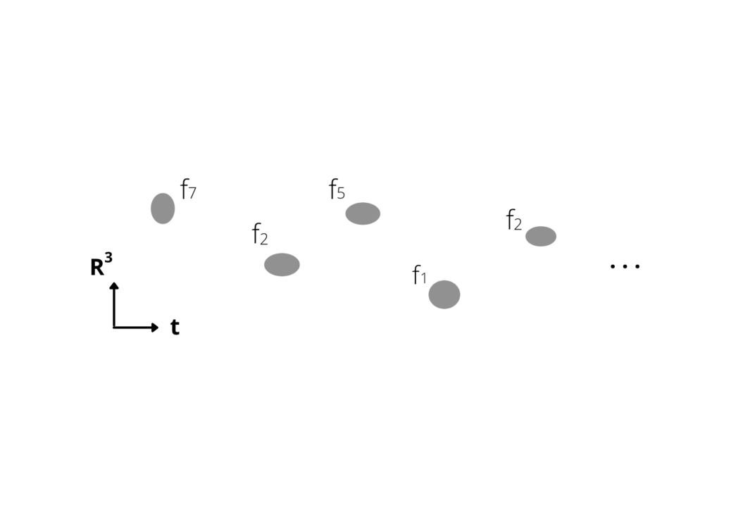
Figure 1: Measurement of a variable $F$. Each blob describes a single measurement event (a chain ionization reaction, hadronic cascade, etc.) occurring at a localized region in spacetime, with the experimental results, $F=f_{7},f_{2},f_{5},f_{1},f_{2}$, etc. The wave functions describing the different measurement events ${\tilde{\Phi}}$ have no overlapping spacetime supports, therefore are orthogonal.

5.1.1 Particle hitting a potential barrier

To clearly grasp the idea of effective spacetime localization of the measurement events, consider a simple particle scattering off a one-dimensional square potential barrier. Even though the plane-wave description yields the correct transmission ($D$) and reflection ($R$) coefficients, as taught in every quantum mechanics course, a time-dependent, wave-packet description of the process shows that the initial rightmoving incoming packet, the transmitted wave packet travelling rightwards and the reflected wave packet travelling backward towards left, do not overlap with each other in spacetime. The absence of the interferences between any two of them is thus seen trivially in the wave-packet description, while it is not obvious in the static, plane-wave formulation of the problem commonly employed. To complete the analogy with (5.7), one may consider measuring the particle at both sides of the barrier. Each time, the particle will appear either on the right or on the left, with average relative frequencies, $D$ and $R$, respectively.

5.1.2 Tonomura’s “double-slit” experiment

The experiment by Tonomura et. al. [12] is a perfectly general type of the measurement process, described by (5.6) $\sim$ (5.8). Before the electron hits the photographic plate, it is described by a wave function $\psi$ having two components coming through the two sides of the filament with positive potential between two plates (acting as a double slit [12]). The measurement takes place at the moment the electron impinges on the photographic screen, and leaves an ionization blot at some $x$.

In this experiment the electron beam is carefully prepared. The electron wave packets, the mean velocity of the electrons and the beam intensity, are such that the average distance between the two successive electrons are (so to speak) $\sim 150\,km$, to be compared with the size of the wave packets ($\sim 1\,\mu m$) and the distance from the source to the screen ($\sim 1.5\,m$). The wave packets of different electrons do not interfere with each other. The electrons do arrive, one by one (Fig. 2).

The normalized expected frequency for different values of $x$ is given by $\sim|\psi(x)|^{2}$, which predicts interference fringes à la Young. They are indeed observed experimentally, after many electron images ($20000\sim 70000$) are collected, see Fig. 2.

Note that different points on the screen (ionization blots) correspond to different spacetime events (different electron arrivals, different measurements): the wave packets of different electrons do not overlap in spacetime. Each ionization blot in Fig. 2 represents a measurement blob of Fig. 1, but here everything is real physics, not a caricature.

In both examples of Sec. 5.1.1 and Sec. 5.1.2, the very possibility of considering, or preparing experimentally, wave-packets of arbitrarily small size, hinges upon the particle nature of the degrees of freedom of our interest. Arbitrarily small wave packets mean that the approximation of neglecting the coherent superposition among different terms in (5.7) can be made as good as we wish.

Figure 2: The pictures correspond, from the top to the bottom, to successive exposures to $10$, $100$, $3000$, $20000$ and $70000$ electrons, respectively. Reproduced from [12], A . Tonomura, J . Endo, T . Matsuda, T . Kawasaki and H. Ezawa, “Dimonstration of single-electron buildup of interference pattern”, American Journal of Physics 57, 117 (1989); doi: 10.1119/1.16104, with the permission of the American Association of Physics Teachers.

5.2 Repeatable, nonrepeatable and intermediate types of state reductions

In an exceptional class of (“repeatable”) experiments, the processes (5.6) $\sim$ (5.8) may look instead as,

$$|\psi\rangle\otimes|\Phi_{0};Env_{0}\rangle = \left(\sum_{n}c_{n}|n\rangle\right)\otimes|\Phi_{0};Env_{0}\rangle$$ (5.22)

$$\longrightarrow \sum_{n}c_{n}|n\rangle\otimes|{\Phi}_{n};Env_{0}\rangle$$ (5.23)

$$\longrightarrow \sum_{n}c_{n}|n\rangle\otimes|{\Phi}_{n};Env_{n}\rangle\;:$$ (5.24)

namely, each of the states of the original microsystem $|n\rangle$ remains factorized from the apparatus-environment state, even though the latter has registered the reading $F=f_{n}$. The state vector reduction (5.21) takes a special form,

$$\left(\sum_{n}c_{n}|n\rangle\right)\otimes|\Phi_{0};Env\rangle\Longrightarrow|m\rangle\otimes|{\Phi}_{m};Env\rangle\;.$$ (5.25)

Namely the measurement leaves the microsystem with a well-defined wave function, $|m\rangle$. This kind of processes is often discussed in textbooks, as a typical “wave function collapse”,

$$|\psi\rangle=\sum_{n}c_{n}|n\rangle\Longrightarrow|m\rangle\;.$$ (5.26)

A process such as (5.25) or (5.26) means that the result of an experiment can be used as the initial condition for subsequent studies of the system, i.e., as a state preparation. This (ideal) type of measurements are known as “repeatable” in the literature.

Even though these represent indeed special class of measurements, they are neither rare nor particularly difficult to realize experimentally, either. More importantly, they play an essential role for the consistency of quantum mechanics (see Sec. 5.1 and Appendix B).

An almost trivial example of a repeatable measurement is a position determination by a little sheet with a tiny hole. If a particle has passed it, its position has been measured. Let us superpose another sheet with a hole at the same position. The particle which passes the first hole passes also the second. But now overlay it with a second sheet with a hole in a different position. The particle which passed the first gets blocked by the second, this time. This over-simplified model describes nonetheless a perfectly valid quantum mechanical measurement, illustrating (5.26) .

Another, more interesting example of the repeatable measurement, is a variation of the standard Stern-Gerlach (SG) experiment with an inhomogeneous magnetic field with gradient in the $z$ direction, with a beam of massive spin $\tfrac{1}{2}$ atoms moving in the $x$ direction.

Let us assume for definiteness that the spin of the atoms is directed towards ${\bf n}$: it is in the state (2.8). As the atoms proceed, their wave packets are divided in two, one going up (spin $s_{z}=\tfrac{1}{2}$) and the other going down (spin $s_{z}=-\tfrac{1}{2}$) .

Upon arrival at the photographic plate the atoms will leave two bands of ionization blots, upper and lower ones, with relative intensities, $|c_{1}|^{2}$ and $|c_{2}|^{2}$. This standard SG experiment is clearly of a generic (not repeatable) type, described by (5.6)$\sim$ (5.8).

Let us now, however, place a concrete block to impede the lower wave packet from proceeding further towards right. On the photographic screen at the end, we will observe just one (upper) band of the images, instead of two. This measurement is still not repeatable.

But now remove the photographic plate (but not the magnetic field and the concrete block). This time apparently nothing will be observed: the measurement is not completed.

Nevertheless, the beam of the atoms which have passed the region of the magnetic field and cement block, contains now only atoms in the spin-up state. Related processes are known as “null measurements” in the literature ; we may coin them as ”half measurements” as well, as only the first half of the experiment - the preparation of the magnetic field and of the cement block has been done, but no final observation of the vertical position of the atoms in arrival on the screen- has been made.

But because of this, the part of the beam which passed the experimental region contains only atoms in the state $s_{z}=\tfrac{1}{2}$, and can be used in subsequent experiments with the known initial wave function, $|\!\uparrow\rangle$. The state-vector reduction has occurred exactly as in (5.25), (5.26). Note that for subsequent studies only the atoms which passed the first experimental region matter.

Still another example of a repeatable measurement is a beam of light impinging on a crystal or a polaroid, which have a given polarization axis, discussed in many textbooks.

However, in more general types of experiments this aspect (the measurement as the state preparation) cannot be maintained. Often the measurement takes place when an incoming electron, photon, proton, atom, etc. triggers a chain ionization process or a hadronic cascade at some point of the measuring device, leaving a particle track on the instrument (registered on time), or an ionization blot on the photographic plate. It might look as if what “collapses” is not the wave function of the incoming electron but the equilibrium state of the macroscopic matter which make the body of the device, from a neutral, uniform state to the one with a particular reading of the measurement result. The incoming electron gets simply lost somewhere. The state-vector reduction takes the general form (5.21): the measurement does not serve as a state preparation for subsequent studies.

For completeness, let us note that the state reduction of repeatable experiments, (5.26), (5.25) where the result of the measurement serves as the preparation of a well-defined quantum state, and general non-repeatable processes, (5.21), in which the original microsystem (or information about it) gets completely lost after the measurement, represent actually only two extremal situations. There exist many intermediate types of experiments in which the information about the original microsystem is only partially maintained (or partially lost), during the measurement . The $\alpha$-particle track in a Wilson chamber, the hadronic cascade in a calorimeter, the particle tracks in a silicon detector, are all examples of these more general types of state reductions. The momentum or energy measurement in high-energy experiments, typically requires not a single spacetime event but a sequence of related sub-events.

We will not make, however, any attempt in this work to formulate and classify these different kinds of measurement processes. The concept of the state-vector reduction as used in Sec. 5, is valid and applies equally well to all these cases.

5.3 Unitarity and linearity

The microscopic state $\psi$

$$|\psi\rangle=\sum_{n}c_{n}|n\rangle\;,$$ (5.27)

if left undisturbed, evolves in time according to the Schrödinger equation,

$$i\hbar\frac{d}{dt}|\psi\rangle=H\,|\psi\rangle\;,$$ (5.28)

($H$ being the Hamiltonian of the system) or as

$$|\psi\rangle\longrightarrow U\,|\psi\rangle=\sum_{n}c_{n}\,U|n\rangle\;,\qquad U=e^{-iHt/\hbar}\;,\quad U^{\dagger}U={\mathbf{1}}\;:$$ (5.29)

it is a linear, unitary evolution. Unitarity means that

$$\langle\psi|\psi\rangle=\sum_{n}|c_{n}|^{2}=1\;,$$ (5.30)

i.e., the state is normalized and its norm is conserved in time. Linearity of evolution means (5.29), i.e., superposition of different states in (5.27) continue to be coherent superposition of the corresponding states, though each term has evolved by the same unitary operator $U$. These properties of pure states are well-known.

During the measurement process, when the microsystem gets in contact with the measuring device, the latter reading the result of the measurement, the time evolution, formally written as (5.7), might still look unitary and linear. However, as we have seen, the wave functions associated with different terms in (5.7) do not overlap in spacetime: it represents a mixed state. The coherent superposition of states is no longer there, see (5.17). Most significantly, the real time evolution of the system is the state-vector reduction, (5.21).

This means that linearity is lost during the measurement.

On the other hand, unitarity is maintained : the sum of all possible outcomes, occurring at different measurements at different times, adds up to unity of the total normalized frequencies, corresponding to the “norm” of the state, (5.7). In terms of the relative frequencies for different outcomes, ${\cal P}_{n}$, unitarity reads

$$\sum_{n}{\cal P}_{n}=1\;,\qquad\sum_{n}|c_{n}|^{2}=1\;,$$ (5.31)

even though different (sometimes the same, but repeated) experimental results $f_{n}$ refer to distinct measurements made at different times.

Note that this is indeed how experimentalists view the meaning of unitarity. Unitarity means that ${\cal N}_{n}/{\cal N}$ , to be identified with the theoretical formula, ${\cal P}_{n}=|c_{n}|^{2}$, should satisfy

$$\sum_{n}{\cal N}_{n}/{\cal N}=1\;,$$ (5.32)

which might look trivial. However, this contains an implicit, important assumption that the experimental device has no systematic bias, and registers all possible results $f_{n}$ with equal efficiency and with no losses. Only in such an ideal measurement setting we can expect that the experimental results ${\cal N}_{n}/{\cal N}$ will approach the theoretical prediction, ${\cal P}_{n}$, at large ${\cal N}$ (e.g., Tonomura’s experiment, Fig. 2).

It is interesting to compare the concept of unitarity in the measurement processes as described here, with a more abstract one, in the conventional thinking based on Born’s rule. The latter means in fact

$$\sum_{n}P_{n}=1\;,$$ (5.33)

i.e., that the total probability for a single experiment to give all possible results $f_{n}$, is unity, and that it is conserved in time. The request (5.33), from the mathematical, logical point of view, appears quite indispensable, and indeed has always been considered sacrosanct in the traditional approach to quantum mechanics.

However, once $P_{n}$ is translated into the physically directly meaningful quantity, ${\cal P}_{n}~{}(=P_{n})$, the expected relative frequencies for various results $f_{n}$ which will be found in distinct measurements and at different times, unitarity as an absolute principle of the conservation of the total probability, may appear to lose part of the aura traditionally accompanying it.

To conclude, one must be cautious in applying the concepts such as linearity or unitarity of the time evolution, valid in the context of pure states, to the measurement processes where entanglement between the microsystem and the measurement device as well as with the whole world, plays an essential role. Their consequences in these, complicated mixed states may well (and indeed, do) look differently from what one is accustomed to from the experiences in pure quantum states kept in isolation.

A few additional remarks on curious subtleties in the concept of unitarity and quantum mechanical predictions are in Appendix B for the interested reader.

5.4 Degenerate eigenvalues

We have assumed in (5.1) that the eigenvalues $f_{n}$ are non degenerate. Existence of one or more $f_{n}$’s which are degenerate, signifies that there are some variable(s) compatible with $F$, and the state is characterized, not only by the eigenvalue $f_{n}$ of $F$ but also by the eigenvalues of those other variables. For simplicity, let us assume that there are two compatible variables, $F$ and $G$, $[F,G]=0$, and that the state $\psi$ is given by

$$|\psi\rangle=\sum_{n,\ell}c_{n,\ell}\,|n,\ell\rangle\;,\qquad F|n,\ell\rangle=f_{n}|n,\ell\rangle\;,\quad G|n,\ell\rangle=g_{\ell}|n,\ell\rangle\;,$$ (5.34)

$$\sum_{n,\ell}|c_{n,\ell}|^{2}=1\,,$$ (5.35)

instead of (5.1).

Now $|n,\ell\rangle\;$ is the state in which the variables $F$ and $G$ have definite values both; it is the standard understanding that these two variables are simultaneously measurable. Let us consider a simultaneous, double measurement of $F$ and $G$. Even though each measurement is a spacetime event, the contemporaneity of the measurements means that they both refer to the same micro system, described by the wave function, (5.34).

The meaning of the contemporaneity of the two compatible measurements, is illustrated well in the example of the system composed two spin $\tfrac{1}{2}$ particles, in the total spin $0$ state, (8.1), (8.3), which will be discussed later in Sec. 8 in relation to the EPR paradox and entanglement. Let us take $F=s_{1\,z}$ and $G=s_{2\,x}$ which commute with each other. In measuring $F$ and $G$ simultaneously, the experimentalists must make sure that they are studying the two spin $\tfrac{1}{2}$ particles, from the same, single decay event - the coincidence check. This guarantees that the two experiments are done on the same state $\psi$; the exact contemporaneity of the two measurements (spacetime events) is immaterial.

Assuming that such simultaneous measurements are done properly, the result is the wave-function collapse,

$$\sum_{n,\ell}c_{n,\ell}\,|n,\ell\rangle\ \otimes|\Phi_{0}\rangle\Longrightarrow|{\tilde{\Phi}}_{m,k}\rangle\;,$$ (5.36)

which generalizes (5.21), where $|{\tilde{\Phi}}_{m,k}\rangle$ is the state of the entangled microsystem-measurement device, labelled by the double reading, $F=f_{m}$, $G=g_{k}$.

[${\mathbbm{Q}}$]:   What if only one of the variables, say $F$, is measured in the state, (5.34)?

In an ideal class of experiments, the measurement of $F$ might leave undisturbed the state with respect to $G$. In the instant $F=f_{n}$ is measured, the wave function collapses as,

$$\sum_{n,\ell}c_{n,\ell}\,|n,\ell\rangle\ \otimes|\Phi_{0}\rangle\Longrightarrow|\psi_{G}\rangle_{n}\otimes|{\tilde{\Phi}}_{n}\rangle\;,$$ (5.37)

where

$$|\psi_{G}\rangle_{n}=\sum_{\ell}c_{n,\ell}\,|n,\ell\rangle\;,\qquad({\rm no~{}sum~{}over}\,\,n)\;.$$ (5.38)

A simple example of this kind of experiment is the measurement of $s_{1\,z}$ in the example of a system composed of two spin $\tfrac{1}{2}$ particles, mentioned above. The measurement of $F=s_{1\,z}$ does not interfere with the state of $G=s_{2\,x}$: the instant $F$ has been found in the state $s_{1\,z}=+\tfrac{1}{2}$, the system will be left with a nontrivial wave function (see (8.3)),

$$|\psi\rangle_{G}=\frac{1}{\sqrt{2}}(|+\rangle-|-\rangle)\;,\qquad s_{2\,x}|\pm\rangle=\pm\frac{1}{2}|\pm\rangle\;.$$ (5.39)

On the other hand, in more general classes of experiments, the measurement of $F$ may influence the state with respect to $G$. In the simple position determination at the final stage of Tonomura’s double-slit experiment [12], the measurement of $F=x$, the horizontal coordinate relevant to the interference fringe (Fig.2), is necessarily accompanied by the determination of $G=y$ (the vertical position of the electron arrival). In other words, the measurement of $F=x$ induces the wave-function collapse both in $F=x$ and in $G=y$.

These two simple examples are sufficient to show that $[{\mathbbm{Q}}]$ is not a sort of question which can be answered based on some general, abstract principles. The answer depends on the details of the measurement settings, as well as on the nature of the variables.

5.5 Macroscopic quantum-mechanical systems

Sometimes discussed in relation with the measurement processes are the so-called macroscopic quantum states. Let us at once note that there are, roughly, two classes of such systems which are to be distinguished [13]. To the first class belong many well-known phenomena such as superfluidity and superconductivity, BE condensed ultracold atoms, and actually, many familiar phenomena in quantum field theories, such as spontaneous symmetry breaking, Higgs mechanism, and so on. The mechanism under which a macroscopic (or an infinite) number of identical bosons, elementary or composite, occupy the same quantum states, and form macroscopic wave functions, is well understood.

A second class of macroscopic (or mesoscopic) quantum states refer to a large number of particles, or a large molecule, which behave quantum-mechanically, exhibiting the phenomena of diffraction, interference, and tunnelling between different macroscopic (mesoscopic) states. This is a fascinating, rapidly developing experimental research area.

A double-slit experiment by using the molecules $C_{60}$ shows an example of such a mesoscopic system [14]; the pair of the SQUID states with macroscopic fluxes of opposite signs, with possible tunnelling between them, are an example of this type of macroscopic quantum systems [13]. A recent construction of a mechanical resonator [15] kept at $T\sim 20$ mK is considered to be a promising start for realizing in the laboratory an analogue of the linear superposition of the “dead and alive cat” states.

None of these phenomena, however, are directly relevant to the question of the measurement problems. The scope of the experimental apparatus is, in a sense, exactly opposite. The task of an measurement device is to pick up the information about the fluctuating quantum mechanical system, and to convert its (unique) reading into a classical state of matter. The wave-function collapse (5.21) is, by definition, a process in which the coherent superposition of the macroscopic experimental-device states gets eliminated.

To close a possible loophole in the argument, however, let us note that, even though a generic, classical body can hardly be characterized as a macroscopic quantum-mechanical system, we must still keep in mind that the distinction between the two (i.e., a “macroscopic quantum state” and a classical state) may not always be sharp. A familiar example is light, which may be regarded as a wave of the classical electromagnetic fields, but it is also a macroscopic quantum state describing the collective motion of photons. A magnet can also be seen as a classical state of matter, but its microscopic description leads us to a quantum-mechanical system consisting of macroscopic number of aligned spins. It is well-known that in a system of infinite degrees of freedom in two or more dimensions, a tunnelling between two degenerate vacua is not possible. The system chooses one of them as the unique vacuum. Spontaneous symmetry breaking is a phenomenon of this kind.

It could be tempting to try to relate the classical uniqueness of the reading of the measurement device to spontaneous symmetry breaking [11]. However, typical quantum measurements such as the Stern-Gerlach experiment (and many others) do not seem to be of this nature.

Our arguments here, on the other hand, tell nothing about (or against) the possibility of finding, or fabricating, macroscopic or mesoscopic quantum mechanical states such as those discussed in [13, 14, 15], outside the context of quantum measurement problems.

5.6 Summary: the main result of this work

Summarizing Sec. 5, the crux of the absence of coherent superposition of different terms in the measuring process, (5.7), is the lack of the overlapping spacetime supports in the associated wave functions. As a result of entanglement between the microsystem described by the wave function $\psi$ and the experimental apparatus (and the environment), the whole system gets rapidly transformed into a mixed state characterized by the diagonal density matrix, (5.19). The result of each measurement is the state-vector reduction, (5.21). The experiments on the state $\psi$, (5.9), produce various results $F=f_{n}$ with relative frequencies, $|c_{n}|^{2}$.

These discussions indeed integrate the arguments of Sec. 2 (see Sec. 2.3 for the summary), where the connection (identification) between theoretical expectation values and the average experimental results were only an assumption.

Combining the results of Sec. 5 (especially, Sec. 5.1) and Sec. 2, indeed, we have been led to the standard quantum mechanical prediction, that measurements on the state $\psi$ give various results $F=f_{n}$ with relative frequency ${\cal P}_{n}=|c_{n}|^{2}$. ${\cal P}_{n}$ is equal to $P_{n}=|c_{n}|^{2}$, the probability that a single measurement gives $F=f_{n}$, according to Born’s rule.

The difference between relative frequencies and probabilities might sound a semantic question, but it is not. Most importantly, what is lacking in Born’s rule is the explanation (i) how the knowledge about quantum fluctuations (the wave function) gets transcribed, through the measurement processes, into the relative frequencies ${\cal P}_{n}=|c_{n}|^{2}$ for the different outcomes $f_{n}$, and (ii) why and how the state-vector reduction takes place, after each measurement.

To the best of the author’s knowledge, the discussions in this work represent the first significant steps towards filling in these gaps, and point towards a more natural interpretation of quantum mechanical laws. See Sec. 10 for further discussions.

The rest of the work, Sec. 6 $\sim$ Sec. 8, is dedicated to a few illustrations of how well-known apparent paradoxes and puzzles in the literature can be naturally explained.

6 Quantum jumps and metastable states

A question often debated is how to reconcile the smooth time evolution of the wave function described by the Schrödinger equation with sudden “quantum jumps”, occurring in radioactive nuclei ($\alpha$ and $\beta$ decays), the spontaneous emission from the excited atoms, and so on.

Let us consider an $\alpha$ decay from a metastable nucleus, $X$,

$${}^{A}_{N}\left(X\right)\Longrightarrow{}^{A-4}_{N-2}\left(Y\right)+\alpha\;,$$ (6.1)

where $N$ is the atomic number and $A$ is the mass number. By considering some population of the nuclei $X$, it seems natural to write the wave function for the system as

$$|\psi\rangle=|X\rangle+|Y\rangle|\alpha\rangle\;.$$ (6.2)

We do not bother to write the coefficients in front of the two terms: their norms are not conserved due to the decay, see below, (6.4). Without going into detail, one can immediately note that the first ($|X\rangle$) corresponds to a bound state, whereas the second ($|Y\rangle|\alpha\rangle$) describes an unbounded system: $\alpha$ is a free particle flying away. Therefore the overlap between the two terms (the interference) is absent. In spite of a writing which may indicate otherwise, (6.2) is not the wave function of a pure state. It is a mixed state.

In many systems of interest such as this, there are certain effects (say, the interaction Hamiltonian, $H_{I}$), which may be regarded as small, and can be treated as perturbations. Examples are: the electroweak interactions or tunnel effects in nuclei, the interactions with radiation fields in atoms, and so on. By first considering the system with the Hamiltonian $H_{0}$, without these interactions, and taking $H_{I}$ into account appropriately as perturbations, and perhaps with the aid of the analytic continuation for the solution of the Schrödinger equation with smoothly varying parameters, it is possible to define the wave function of the metastable state, $|X\rangle$ (see for instance Chap. 13 of [1]). The state being metastable, its energy has a small imaginary part,

$$E=E_{R}-i\,\frac{\Gamma}{2}\;,$$ (6.3)

where $\Gamma$ represents the total decay rate per unit time (or the level width), and $\tau=\hbar/\Gamma$ is the mean lifetime. The wave function has a time dependence,

$${\tilde{\psi}}_{X}(t)=e^{-iEt/\hbar}{\tilde{\psi}_{X}(0)}=e^{-iE_{R}t/\hbar}e^{-\Gamma t/2\hbar}{\tilde{\psi}_{X}(0)}\;.$$ (6.4)

Now how can one reconcile such a smooth time dependence with sudden quantum jumps, such as $\alpha$ decay, a spontaneous emission of photons from an excited atom? This sort of question, probably mixed up with a philosophical confrontation between Heisenberg’s (based on the matrix mechanics, with emphasis on the transition elements) and Schrödinger’s (with the wave function obeying smooth differential equations) views of quantum mechanics, dominated the earlier debates on quantum mechanics .

A little thought tells us that the nature (hence, the solution) of the problem is basically the same as that of the measurement problems considered in Sec. 5. The detection of these quantum jumps, e.g., the observation of an $\alpha$ particle suddenly appearing and leaving a track in a Wilson chamber, is a measurement as any other. Of course, in general, a spontaneous decay of a metastable nuclei, atom or molecule, occurs even without a calibrated measuring device waiting for the decay products to appear. But there is a common feature shared with the measurement processes. The quantum jumps are caused by some elementary interactions in $H_{I}$ such as the photon emission by the electron in an excited atomic level, a Fermi interaction of a neutron, or an $\alpha$ particle hitting the Coulomb barrier inside a nucleus, which are all spacetime events. In this sense, these pointlike, eventlike processes capture one of the fluctuating states in the original metastable system, exactly as in a measurement process discussed in Sec. 5. As such, the exact timing of a spontaneous quantum jump, as well as the specific details of the final states in each decay, cannot be predicted. They are manifestation of the quantum fluctuations of the system. Their averages are, however, described by ${\tilde{\psi}}$.

There is, however, a crucial difference between the general measurement processes discussed in Sec. 5 and the spontaneous, quantum jumps. It is the fact that in the former case, the wave function $\psi$ in (5.1) describes a true quantum state. It never spontaneously collapses (i.e., decays) to one of the fluctuating states, if left undisturbed. In a measurement process, it is the interactions with macroscopic, measuring instruments, sensitive to the microscopic state described by $\psi$, that pick up one of the possible fluctuating states, experiment by experiment, making the microsystem appear to jump into one of the eigenstates, as in (5.21).

From the very way the wave function $\tilde{\psi}$ for a metastable state is defined, where $\Gamma$ represents the total decay rates of all possible decay processes of the parent particle, it is quite clear that $\tilde{\psi}$ represents an effective description of the metastable “quantum state”, in which the coarse-grained time dependence (decay events) has been smoothed out. It does not have the same status as the wave function of a genuine quantum state $\psi$, (5.1).

In conclusion, the conundrum of apparent impossibility of reconciling the smooth time-dependent Schrödinger equation with quantum jumps, appears to have been caused by the confusion between the concept of the true wave function $\psi$ and that of an effective “wave function” for a metastable “state”, ${\tilde{\psi}}$.

6.1 Atomic transitions: other examples of quantum jumps

Spontaneous emission of photons from an excited atom is a typical quantum jump, as discussed above. Just to be complete, let us note that the two other kinds of atomic transitions, absorption-excitation and stimulated emission, are also both eventlike processes, sharing common features with the decay of metastable states, as well as with the measurement processes. Note, for instance, that in the photoelectric effect, absorption of the photon and excitation-ionization of the $Li$ atoms in the target plate, is an eventlike process, serving as a measurement of the incoming-photon energy .

7 Schrödinger’s cat

In the discussion involving Schrödinger’s cat, the initial “wave function” is a combination (6.2), between the undecayed nucleus $|X\rangle$ and the state after decay, $|Y\rangle|\alpha\rangle$. To maximally simplify the discussion and to go directly into the heart of the problem, let us eliminate altogether the intermediate, diabolic device which upon receipt of the $\alpha$ particle leads to the poisoning of the cat, and treat the cat directly as the measuring device, $|\Phi\rangle$. When it detects the $\alpha$ particle, it dies; when it does not, it remains alive. There are two terms in the measurement process, (5.6), (5.7), which here reads

$$|\psi\rangle\otimes|\Phi_{0}\rangle=\left(|X\rangle+|Y\rangle|\alpha\rangle\right)\otimes|\Phi_{0}\rangle$$ (7.1)

$$\longrightarrow |X\rangle\otimes|\Phi^{(alive)}\rangle+|Y\rangle|\alpha\rangle\otimes|\Phi^{(dead)}\rangle\;$$ (7.2)

(we dropped also the rest of the world, $|Env\rangle$). Such a process appears to lead to the superposition of the dead and alive cat, which is certainly an unusual notion, difficult to conceive, to say the least.

Actually, there are at least three elements (of abuse/misuse of concepts) in this argument, each of which individually invalidates it, eliminating the notorious conundrum.

The first is the fact, as seen in the last section, that the “state” of the undecayed nucleus, $X$, is not a pure state. The “wave function” ${\tilde{\psi}}_{X}$ describing it is not a proper wave function but an effective one, in which the coarse-grained time dependence has been averaged out. Second, the linear superposition $|\psi\rangle\sim|X\rangle+|Y\rangle|\alpha\rangle$, as discussed around (6.2), does not represent a pure state (even if we ignore the problem of $|X\rangle$ itself), but a mixed state: $|Y\rangle|\alpha\rangle$ represents the decay product of $|X\rangle$, unbounded and incapable of interfering with the latter.

Finally, even putting aside these two issues, the process (7.1), (7.2) has clearly all the characteristics of a general measurement process discussed in Sec. 5. As explained there, the wave functions describing the two terms of (7.2) lack overlapping spacetime supports. There are no interferences between the terms involving the coupled system involving the microsystem and the classical measurement device (the cat here). The formula (7.2) represents a mixture.

Equivalently, and perhaps more intuitively, one can use the notion of the wave-function collapse. The exact timing of the spontaneous $\alpha$ decay cannot be predicted, as it reflects a quantum fluctuation. But the moment an $\alpha$ particle is emitted, and the cat gets hit by it (the instant of the measurement), the wave function collapses,

$$|\psi\rangle\otimes|\Phi_{0}\rangle\Longrightarrow|Y\rangle|\alpha\rangle\otimes|\Phi^{(dead)}\rangle\;.$$ (7.3)

Recapitulating, Schrödinger’s cat paradox, as it has been formulated originally, was concocted by improper use of concepts such as the superposition principle, unitary and linearity of evolution, and mixing up the pure and mixed states. Any apparently paradoxical feature disappears, once these errors are taken into account .

This being so, it is an entirely different question whether or not quantum-mechanical superposition of macroscopic states (a distant analogue of the superposed dead and alive cat), as those discussed briefly in Sec. 5.5, can be somehow realized experimentally.

8 Quantum entanglement and the EPR “paradox”

Let us consider now the famous Einstein-Podolsky-Rosen setting (in Bohm’s version) of a total spin $0$ system decaying into two spin $\tfrac{1}{2}$ particles flying away from each other. The (spin) wave function is given by

$$|\Psi_{0}\rangle=\frac{1}{\sqrt{2}}\left(|\!\uparrow\rangle|\!\downarrow\rangle-|\downarrow\rangle|\!\uparrow\rangle\right)$$ (8.1)

​ where $|\!\uparrow\rangle$ ($|\!\downarrow\rangle$) represents the state of the 1st and 2nd spins, $s_{1,z}=\pm\tfrac{1}{2}$, $s_{2,z}=\pm\tfrac{1}{2}$. As spin components of the single spins do not commute with the total spin ${\mathbbm{S}}_{tot}^{2}$, e.g.,

$$[{\mathbbm{S}}_{tot}^{2},s_{1,i}]\neq 0\;,\quad[{\mathbbm{S}}_{tot}^{2},s_{2,j}]\neq 0\;,\qquad i,j=x,y,z\;,$$ (8.2)

$s_{1\,z},s_{2\,y}$, etc., are fluctuating between $\pm\tfrac{1}{2}$ in the state $\Psi_{0}$. Note that $\Psi_{0}$ can be written in infinitely many different ways, reflecting possible fluctuation modes of the subsystems,

$$|\Psi_{0}\rangle=\frac{1}{\sqrt{2}}\left(|+\rangle|-\rangle-|-\rangle|+\rangle\right)=\frac{1}{2}\left[\,|\!\uparrow\rangle(|+\rangle-|-\rangle)-(|+\rangle-|-\rangle)|\!\uparrow\rangle\,\right]=\ldots\;.$$ (8.3)

It is of fundamental importance to realize that such (correlated) fluctuations of the two subsystems - quantum entanglement - are present however distant the subsystems may be, and even if they might be relatively spacelikely separated. Nothing in $\Psi_{0}$ tells us otherwise. Nothing in quantum mechanical law says that such entanglements are present only when the subsystems are nearby, e.g., less than $10^{-8}$ cm, or less than $10^{+28}$ cm. Simply, quantum mechanics does not contain any fundamental parameter with the dimension of a length .

In the EPR-Bohm experiment, this means that an experimental result at one arm, say, $s_{1\,z}=\tfrac{1}{2}$, might appear to imply “instantaneously” that the second experiment at the other arm would be in the state $s_{2\,z}=-\tfrac{1}{2}$, even before it is actually performed, and however distant they may be. This could sound paradoxical (sometimes the term “quantum nonlocality” is used). The second experimentalist, not having access to the first experiment, might have (should have?) expected to find the results $s_{2\,z}=\pm\tfrac{1}{2}$, a priori with equal probabilities.

This kind of argument has led to the introduction of the hidden-variable hypothesis (see [4] for discussions), although such a deduction was not actually justified. We limit ourselves here to noting that this argumentation had several logical flaws. First, the contemporaneity of the two experiments is not really an issue: the experimentalists must just ensure that they are studying the two spin $\tfrac{1}{2}$ particles from the same decay event - the coincidence check. The exact time ordering, which depends on the reference system chosen, cannot matter. In any case, as the two subsystems are spacelikely separated, it is untrue that the second experimentalist would know instantaneously the result of the first experiment, or actually, even whether or not the first measurement has been indeed performed. The information transmission is itself a dynamical process. Finally, the two “simultaneous” experiments would capture only those states of the two subsystems fluctuating according to the entangled wave function, (8.1), (8.3). In conclusion, for the second experimentalist the system presents itself as a mixture with an unknown density matrix. He (she) simply does not know what to expect. There was no paradox.

Coming back to physics, the first experimental result $s_{1\,z}=\tfrac{1}{2}$ does imply, instantaneously (whatever it may mathematically mean), that the other spin is in the state $|{\downarrow}\rangle=\tfrac{1}{\sqrt{2}}(|+\rangle-|-\rangle)$. This follows from the explicit form of the wave function (8.1), (8.3) . But unless the second measurement is done, any components of the second spin other than $s_{2\,z}$ are still fluctuating . Thus if the two Stern-Gerlach type experiments are performed at the two ends simultaneously, by using the magnets directed to generic directions ${\bf a}$ and ${\bf b}$, they would find, experiment by experiment, apparently random results, such as $(s_{1\,a},s_{2\,b})=(\tfrac{1}{2},\tfrac{1}{2}),(\tfrac{1}{2},-\tfrac{1}{2}),(-\tfrac{1}{2},-\tfrac{1}{2})$, etc. But their fluctuation average is encoded in $\Psi_{0}$:

$$\langle\Psi_{0}|s_{a}s_{b}|\Psi_{0}\rangle=-\frac{1}{4}\cos\theta_{a,b}=-\frac{1}{4}\,{\bf a}\cdot{\bf b}\;.$$ (8.4)

Renowned inequalities by Bell (1960) [4] for this system, and CHSH inequalities [19] for analogous, polarization correlated photon pair experiments, show that hidden-variable models, independently of the details, cannot simulate completely quantum mechanical predictions based on formulas such as (8.4), which encode the entanglement information. Beautiful experiments by Aspect et. al. (1981) [20] have subsequently demonstrated that, whenever the hidden-variable alternatives and quantum mechanics give discrepant predictions (for certain sets of magnet orientations or polarizer axes), the experimental data confirm quantum mechanics, disproving the former.

See also Chiao et. al. (1995) [21] for a series of related experiments and discussions.

8.1 Entanglement among more than two particles

An amusing variation of the EPR-Bohm experiment to the one with more than two particles was considered by Mermin [22], which (apparently) shows a further mysterious and paradoxical feature of quantum entanglement . Consider three spin-$\tfrac{1}{2}$ particles in the state

$$\ket{\Psi_{M}}=\psi({\bf r}_{1},{\bf r}_{2},{\bf r}_{3})\,\frac{1}{\sqrt{2}}\left(\ket{\uparrow}\ket{\uparrow}\ket{\uparrow}-\ket{\downarrow}\ket{\downarrow}\ket{\downarrow}\right)\,,$$ (8.5)

with the three particles receding from each other (e.g., they are the decay product of some parent particle), each pair getting separated by a spacelike distance. Let us consider four operators ($\sigma$’s being twice the spin operators, $s_{1,x}=\tfrac{1}{2}\sigma_{1,x}$, etc.),

$$M_{1}=\sigma_{1\,x}\,\sigma_{2\,y}\sigma_{3\,y},\quad M_{2}=\sigma_{1\,y}\,\sigma_{2\,x}\,\sigma_{3\,y},\quad M_{3}=\sigma_{1\,y}\,\sigma_{2\,y}\,\sigma_{3\,x},\quad M_{4}=\sigma_{1\,x}\,\sigma_{2\,x}\,\sigma_{3\,x}\;,$$ (8.6)

which commute with each other. A remarkable property of state (8.5) is that it is a simultaneous eigenstate of all four operators,

$$M_{1}\,\ket{\Psi_{M}}=M_{2}\,\ket{\Psi_{M}}=M_{3}\,\ket{\Psi_{M}}=\ket{\Psi_{M}}\,,$$ (8.7)

and

$$M_{4}\,\ket{\Psi_{M}}=-\ket{\Psi_{M}}\;,$$ (8.8)

as can be easily verified. Now consider measuring $M_{1}$: simultaneous measurements of commuting variables $\sigma_{1\,x}$, $\sigma_{2\,y}$ and $\sigma_{3\,y}$. Each of them will yield $\pm 1$ as a result: let us call them $m_{1\,x}$, $m_{2\,y}$, $m_{3\,y}$, respectively. Because of the first of (8.7), the triplet of the outcomes will satisfy

$$m_{1\,x}\,m_{2\,y}\,m_{3\,y}=1\;.$$ (8.9)

Similarly, other triple experiments for $M_{2}$, $M_{3}$, and $M_{4}$ will give results,

$$m_{1\,y}\,m_{2\,x}\,m_{3\,y} =1\;,$$ (8.10a)

$$m_{1\,y}\,m_{2\,y}\,m_{3\,x} =1\;,$$ (8.10b)

$$m_{1\,x}\,m_{2\,x}\,m_{3\,x} =-1\;.$$ (8.10c)

Now, as each of the $m$’s take only values $\pm 1$, and because of the crucial minus sign in (8.10c), the results (8.9), (8.10a), (8.10b), (8.10c) are mutually incompatible! Is quantum mechanics inconsistent?

Actually, we have been a little too hasty in jumping to a wrong conclusion. We incorrectly regarded $m_{3\,y}$ appearing in (8.9) and in (8.10a) as the same number, but this is not at all guaranteed. Similarly for $m_{1\,x}$ in (8.9) and in (8.10c). The point is that the triple measurement for $M_{1}$ (which yields (8.9)) and another triple experiment for $M_{2}$ (which gives $m$’s satisfying (8.10a)), for instance, cannot be performed simultaneously, in spite of the fact that the operators $M_{1}$ and $M_{2}$ commute. As $[\sigma_{1\,x},\sigma_{1\,y}]\neq 0$, the experimentalist at site 1 cannot measure them simultaneously. More generally, even though the four operators $M_{1},\ldots,M_{4}$ commute with each other, observation of such composite variables, each of which requires three “simultaneous” measurements taking place in different sites, cannot be simultaneously performed, against the standard lore of quantum mechanics . Stated more precisely, relations (8.9), (8.10a), (8.10b), (8.10c) necessarily refer to four different (triple-measurement-) events, with unrelated $m$’s. They should have been written as

$$m_{1\,x}\,m_{2\,y}\,m_{3\,y}=1\;,\quad m_{1\,y}^{\prime}\,m_{2\,x}^{\prime}\,m_{3\,y}^{\prime}=1\;,\quad m_{1\,y}^{\prime\prime}\,m_{2\,y}^{\prime\prime}\,m_{3\,x}^{\prime\prime}=1\;,\quad m_{1\,x}^{\prime\prime\prime}\,m_{2\,x}^{\prime\prime\prime}\,m_{3\,x}^{\prime\prime\prime}=-1\;.$$ (8.11)

There is no inconsistency whatsoever, among the four results.

This system was presented in [22] as a case in which the discrepancy between a hidden-variable theory and quantum mechanics can be seen more sharply than in the EPR experiment/Bell’s inequalities where statistical results of many measurements are needed to discriminate between the two types of theories. The idea would be that the particular set of the hidden variables $\lambda$, supplementing $\Psi_{M}$, which give rise to the results (8.9), (8.10a), (8.10b), would necessarily predict $M_{4}=m_{1\,x}\,m_{2\,x}\,m_{3\,x}=+1$, contradicting the quantum mechanical prediction, (8.10c), with a single experiment!

Actually, such an argument neglects the quantum mechanical aspect of this process we discussed above. The four triple measurements $M_{1}$, $M_{2}$, $M_{3}$, $M_{4}$ necessarily refer to four distinct experiments (four different three-particle decay events), and the state $|\Psi_{M}\rangle$ is such that the results of these experiments satisfy (8.11), each of $m$’s, $m^{\prime}$’s, $m^{\prime\prime}$’s and $m^{\prime\prime\prime}$’s being equal to $\pm 1$. Any plausible hidden-variable model must be such that at least these conditions are correctly simulated. It would not be surprising to find a result which contradicts quantum mechanics, if an assumption violating the principles of quantum mechanics were used to get it .

9 Universe and quantum measurements

Before concluding, let us briefly wander into a few general but related issues which our considerations on quantum measurements have illuminated. Reviews on the concepts of pure and mixed states, and related questions of factorizatioin versus entanglement in Sec. 3 and Sec. 4 have brought us to think of the universe as a large (today) single quantum system (“the wave function of the universe”), which is in an entangled, mixed state.

Massive bodies in it (galaxies, stars, planets, objects on Earth) generally behave classically (i.e., as mixed entangled systems characterized by decoherence [8, 9].) Pure quantum states however occur in Nature (i.e., in our universe) in the form of cosmic rays in the interstellar (intergalactic) spaces: they are free particles such as neutrinos, photons and ultra high-energy protons . They are produced in astrophysical phenomena, stars, supernova, etc., and travel freely, except under adiabatic effects of gravitational and magnetic fields of galaxies. Cosmic Microwave Background (CMB) (and dark matter) at $T\simeq 2.7$K ($T_{DM}=?$) do not disturb them significantly.

Pure states occur naturally also on Earth, due to radioactivity ($\alpha$, $\beta$ and $\gamma$ decays) of unstable nuclei. Unless intercepted, these $\alpha$ particles, electrons and photons, are free particles. Their studies indeed led to the discovery of quantum mechanics between the end of the 19th century and the early 20th century . Cosmic-ray physics also played an important role in the development, for the same reason: they were sources of pure quantum states. The pure states are today also artificially produced and studied in isolated pockets in the world - physics laboratories on Earth with good vacuum technology and accelerators.

As discussed in Sec. 5, quantum measurement is a special procedure of coupling (entangling) various pure states (particles) produced artificially in the laboratories, or (primary or secondary) cosmic rays hitting Earth, to particular kinds of mixed-state bodies (the experimental devices) in entanglement with the environment. The latter has, typically, the characteristics of an ionization chamber, to be triggered by the initial spacetime eventlike interactions (which capture the fluctuating quantum state of the microsystem under study), chain-multiply and amplify enormously the result of the initial triggering-interactions. The measurement result is now in the form of particular, entangled mixed (i.e., classical) states with the reading of the measurement result.

The quantum measurement processes may thus be seen as a very special, controlled way of reproducing what happens constantly in Nature: the loss of factorization and pure-state nature of a subsystem, via interactions (entanglements) with surrounding background, into a mixture.

10 Summary and conclusion

The key observation of this work that the basic entities (the degrees of freedom) of our world are various types of particles, leads to the idea that each measurement, at its core, is a spacetime, pointlike event. The crux of the absence of coherent superposition of different terms in the measuring process (5.7) is, indeed, the consequent lack of the overlapping spacetime supports in the associated wave functions, instant after measurement which is the process of entanglement between the microsystem and the experimental device and the environment. It is in this sense the expression (5.7) represents a mixed state. But it also implies that the aftermath of each measurement corresponds to a single term of (5.7). This (also empirical) fact, is known as the “wave-function collapse”, or the state-vector reduction.

The discussions of Sec. 5 have led to the diagonal density matrix, (5.19). In particular, the information encoded in the wave function $|\psi\rangle=\sum_{n}c_{n}|n\rangle$ has been transferred via entanglement with the experimental device and environment into the relative frequencies for finding the experimental results $F=f_{n}$, ${\cal P}_{n}=|c_{n}|^{2}$. Combined with the equality between ${\cal P}_{n}=|c_{n}|^{2}$ (the relative frequencies) and $P_{n}=|c_{n}|^{2}$ (the probabilities), reviewed in Sec. 2, our results represent the first steps towards filling the logical gaps in Born’s rule, explaining the state-vector reduction, and pointing towards a more natural interpretation of quantum mechanics.

Our discussions do confirm the standard Born rule as a concise way of summarizing the predictions of quantum mechanics. But the fact that it is formulated in terms of the “probability certain result is found in an experiment”, which might (or might not) be eventually performed - perhaps by an experimentalist with a Ph D - has always caused confusion and conceptual difficulties .

In ultimate analysis, the problem of Born’s rule is the fact that it presumes a human intervention.

We instead take the quantum fluctuations described by the wave function as real, and propose that they represent the fundamental laws of quantum mechanics. They are there, independently of any experiments, and in fact, whether or not we human beings are around . In case a measurement is done, the good experimental device will faithfully reflect them, giving in general an apparently random outcome each time. This is as it should be, even though the average-over-experiments-result can be predicted, as the fluctuation averages are encoded in the wave function.

What we propose here is a slightly unconventional way of interpreting quantum mechanical laws. Indeed, the solid textbook materials and the standard methods of analysis in quantum mechanics, all remain unchallenged. After all, we know that quantum mechanics is a correct theory. The new perspective, however, suggests us to put less emphasis in the discussion of quantum mechanics, on certain familiar concepts such as probability, statistical ensembles, Copenhagen interpretation, etc., which historically guided us, but also caused misunderstandings and introduced clouds in the discussion on quantum mechanics, for many years.

Accepting the quantum fluctuations described by the wave function as real, we simply give up pretending, or demanding, that in a fundamental, complete theory describing Nature the result of each single experiment should necessarily be predictable.

As the known structures of our universe (including galaxies, stars, planets and ourselves) are likely to have grown out of uncontrollable quantum density fluctuations at some stage of the inflationary universe, as cosmologists tell us today, this is perhaps a healthy attitude to take, to attain the proper understanding of the quantum laws of Nature, which have far-reaching consequences in all present and future science domains in physics and beyond, from biology and chemistry, quantum information and quantum computing, and possibly, to the brain science.

Appendix A Proof of ${\cal P}_{n}=P_{n}$

Requiring the expectation values of various powers of $F$, (2.25), to be equal to the experimental expected frequency averages, (2.26), for $N=1,\ldots,D$, one finds

$$\sum_{n=1}^{D}f_{n}^{N}\,({\cal P}_{n}-|c_{n}|^{2})=0\;,\qquad N=1,\ldots,D\;.$$ (A.1)

This can be written as

$$\sum_{n=1}^{D}V_{mn}\,d_{n}=0\;,\qquad d_{n}\equiv{\cal P}_{n}-|c_{n}|^{2}\;,\qquad m=1,\ldots,D$$ (A.2)

where $V_{mn}\equiv(f_{n})^{m}$ is a Vandermonde matrix. As its determinant

$$\det V=(\Pi_{n=1}^{D}f_{n})\,\,\Pi_{1\leq n<m\leq D}(f_{m}-f_{n})$$ (A.3)

is nonvanishing, we find

$$d_{n}=0\;,\qquad.^{.}.\quad{\cal P}_{n}=|c_{n}|^{2}=P_{n}\;,\qquad n=1,2,\ldots,D\;.$$ (A.4)

Appendix B Unitarity and measurements

An attentive reader may have noted certain subtleties in the concept of unitarity and measurements. Namely, different expressions of unitarity, (5.31) for the sum of the relative frequencies, (5.32) for the normalized sum of all possible experimental outcomes, and (5.33), the total probability, all look trivial, each in its own way! Even the conservation of the norm of the state may sound suspicious, since a quantum state is defined by the ray of the vector in Hilbert space: its norm is unphysical.

What unitarity tells us is that, once the norm of the state $\psi$ is fixed by convention, and the states in the base $\{|n\rangle\}$ are chosen to be orthonormal, then the evolution $|\psi\rangle\to U|\psi\rangle$ and $c_{n}|n\rangle\to c_{n}U|n\rangle$, maintain the norm of each, $U=e^{-iHt/\hbar}$ being a unitary operator. It follows that each $|c_{n}|^{2}$, their sum, $\sum_{m}|c_{m}|^{2}$, thus the ratio $|c_{n}|^{2}/\sum_{m}|c_{m}|^{2}$, are all $t$ independent. This is welcome, since verification of the predictions on various probabilities (Born’s rule) requires repeated experiments performed at different times. The predictions in terms of the relative frequencies, and the experimental results, refer both directly to the repeated events occurring at different instants. An identical state $|\psi\rangle$ must be prepared ad hoc each time (e.g. by using a repeatable experiment), but once prepared, $|\psi\rangle$ may be allowed to wait, before being sent to the actual experiment region, for an arbitrary amount of time. The start time should not be essential. This is consistent, as an experimental test in quantum mechanics involves (in principle) an infinite number of repeated measurements. For instance, one may throw away the first hundred events from the collection of Tonomura’s electron images Fig. 2: the final result remains the same.

As we saw in Sec. 5, during the measurements, where the microsystem gets entangled with the apparatus-environment state, leaving a mixed state without coherent superposition of the different terms, unitarity $\sum{\cal P}_{n}=1$ remains valid, even though each experimental result $F=f_{n}$ refers explicitly to experimental event which occurred at different time, and each is accompanied by state-vector reduction.

Appendix C Quantum mechanics and Minkowski spacetime

Our key observation that each measurement is at its core a spacetime event occurring at some $(x_{1},x_{2},x_{3},t)$, explains the absence of the overlap in spacetime supports in the wave functions corresponding to different terms in (5.7). This, of course, does not imply that these variables, including the time $t$, are treated as dynamical variables. In spite of a few existing debates, the time $t$ is not a dynamical variable in quantum mechanics.

The spacetime coordinates $(x_{1},x_{2},x_{3},t)$ represent the frame of the Minkowski spacetime in which all particles move. In particular, the time $t$ is a common (time) coordinate for describing the time evolution of all particles present in the system. Actually, the same can be said of the space coordinates $(x_{1},x_{2},x_{3})$, even if the confusion often made between them and the position operators (and their eigenvalues) of the particles obscures this fact. For instance, the wave function of a system of two particles is a function $\psi({\bf q}_{1},{\bf q}_{2},t)$ of six position operators, whereas the fixed space coordinates are always just $(x_{1},x_{2},x_{3})$. The latter is the spectrum for both $({\bf q}_{1})_{x,y,z}$ and $({\bf q}_{2})_{x,y,z}$. The position variables ${\bf q}_{i}$’s fluctuate; $(x_{1},x_{2},x_{3})$ do not.

That there is a basic symmetry between the space and time coordinates even in nonrelativistic quantum mechanics, is actually well known from the quantization rules

$$E\to i\hbar\frac{\partial}{\partial t}\;,\qquad{\bf p}\to-i\hbar\nabla\;,$$ (C.1)

for energy and momentum, which can be cast in a relativistically covariant form,

$$P_{\mu}\to i\hbar\frac{\partial}{\partial x^{\mu}}\;,\qquad x^{\mu}=(t,x_{1},x_{2},x_{3})\;.$$ (C.2)

Such a structure is what makes the generalization of quantum mechanics to relativistic quantum mechanics (the Dirac and Klein-Gordon equations replacing the Schrödinger equation) and to relativistic quantum field theories (QFT), at all possible. It is within this last framework (QFT) that the standard model of the fundamental (strong and electroweak) interactions has been successfully constructed.

Without going into detail, let us recall also that three important properties of quantum mechanics, the spin-statistics connection, locality and causality, all require relativistic-QFT considerations for their proof. See, for instance, Landau-Lifshitz, Vol. 4 [16] for the first, and Peskin et. al. [17], for the second and third.

As a final remark, we recall that the simple form (C.1) of the momentum operator as a differential operator with respect to the canonically conjugate position variable, is valid with any coordinate choice, but only among the Cartesian coordinates but not in curvilinear ones (see, e.g., Sec. 7.8 of [1] for a review), suggesting a key role the flat Minkowski spacetime plays in the standard quantum mechanics framework.

Important physics arises from quantum mechanics (quantum field theories) in the presence of the spacetime curvature, gravity and general relativity. Famous examples are those in black-hole-physics context (e.g., Bekenstein entropy, Hawking radiation), and also the problem of structure formation in our universe which is becoming an essential element of cosmology today. These issues are however beyond (and in our understanding, outside) the scope of the present work.

References

- [1] K. Konishi and G. Paffuti, “Quantum Mechanics: A New Introduction”, Oxford University Press (2009).
- [2] J. A. Wheeler, W. H. Zurek, “Quantum Theory and Measurement”, Princeton NJ: Princeton University Press (1983).
- [3] A. Peres, “Quantum Theory: Concepts and Methods”, Dordrecht/Boston/London: Kluwer (1995).
- [4] J. S. Bell, “Speakable and unspeakable in quantum mechanics”, Cambridge University Press (1987).
- [5] P. A. M. Dirac, “Principles of Quantum Mechanics”, Oxford University Press (1958).
- [6] J. Fröhlich, “A Brief Review of the ETH-Approach to Quantum Mechanics”, 2020, In: Anantharaman N., Nikeghbali A., Rassias M.T. (eds) Frontiers in Analysis and Probability. Springer, Cham.
- [7] J. Schwinger, “On Gauge Invariance and Vacuum Polarization”, Phys. Rev.,82 (1951) pp. 664–679.
- [8] W. H. Zurek, “Decoherence, einselection, and the quantum origins of the classical,” Rev. Mod. Phys. 75, 715-775 (2003) doi:10.1103/RevModPhys.75.715 [arXiv:quant-ph/0105127 [quant-ph]].
- [9] E. Joos, H. D. Zeh, C. Kiefer, D. Giulini, J. Kupsch, I. O. Stamatescu, “Decoherence and the Appearance of a Classical World in Quantum Theory”, Springer, 2002, and references therein.
- [10] D. Frauchiger, R. Renner, “Quantum theory cannot consistently describe the use of itself”, Nature Communications Vol. 9, Article number: 3711 (2018).
- [11] A. E. Allahverdyan, R. Balian, T. M. Nieuwenhuizen, “Understanding quantum measurement from the solution of dynamical models”, Phys. Rep. 525 (2013) 1-166. arXiv:1107.2138.
- [12] A . Tonomura, J . Endo, T . Matsuda, T . Kawasaki and H. Ezawa, “Dimonstration of single-electron buildup of interference pattern”, American Journal of Physics 57, (1989) 117.
- [13] A. J. Leggett, “Macroscopic Quantum Systems and the Quantum Theory of Measurement”, Suppl. of the Progress of Theoretical Physics, 69 (1980) 80.
- [14] M. Arndt, O. Nairz, J. Vos-Andreae, C. Keller, G. van der Zouw, A. Zeilinger, “Wave-particle duality of molecules”, Nature 401 (1999) 680.
- [15] A. D. O’Connell, et. al., “Quantum ground state and single-photon control of a mechanical resonator”, Nature, 464(7289) (2010) 697.
- [16] V. B. Berestetskii, L. P. Pitaevskii and E. M. Lifshitz, “Quantum Electrodynamics”, Landau and Lifshitz Course of Theoretical Physics, Vol. 4 (1982).
- [17] M. E. Peskin and D. V. Schröder “An Introduction to Quantum Field Theory”, (New York, Addison-Wesley, 1995).
- [18] S. Tomonaga, “Quantum Mechanics”, Vol. II, North Holland (1968).
- [19] J. F. Clauser, M. A. Horne, A. Shimony, R. A. Holt, “Proposed experiment to test local hidden-variable theories”, Phys. Rev. Lett., 23 (15): 880 (1969).
- [20] A. Aspect, P. Grangier, G. Roger, “Experimental realization of Einstein-Podolsky-Rosen-Bohm Gedankenexperiment: A new violation of Bell’s inequalities”, Phys. Rev. Lett. 49 (1981) 91.
- [21] R. Y. Chiao, P. G. Kwiat, A. M. Steinberg, “Quantum Nonlocality in Two-Photon Experiments at Berkeley”, arXiv:quant-ph/9501016, and references therein.
- [22] D. Mermin, “Quantum mysteries revisited”, (1990). American Journal of Physics, 58, 731.