Prediction of Large Magnetic Moment Materials With Graph Neural Networks and Random Forests

Abstract

Magnetic materials are crucial components of many technologies that could drive the ecological transition, including electric motors, wind turbine generators and magnetic refrigeration systems. Discovering materials with large magnetic moments is therefore an increasing priority. Here, using state-of-the-art machine learning methods, we scan the Inorganic Crystal Structure Database (ICSD) of hundreds of thousands of existing materials to find those that are ferromagnetic and have large magnetic moments. Crystal graph convolutional neural networks (CGCNN), materials graph network (MEGNet) and random forests are trained on the Materials Project database that contains the results of high-throughput DFT predictions. For random forests, we use a stochastic method to select nearly one hundred relevant descriptors based on chemical composition and crystal structure. This gives results that are comparable to those of neural networks. Our findings suggests that magnetic properties are intrinsically more difficult to predict than other DFT-calculated properties. The comparison between the different machine learning approaches gives an estimate of the errors for our predictions on the ICSD database. Validating our final predictions by comparisons with available experimental data, we found 15 materials that are likely to have large magnetic moments and have not been yet studied experimentally.

I Introduction

In recent years, materials informatics and machine learning methods have been introduced in the search for materials with specific properties, such as high-temperature superconductors [1], photovoltaics [2], radiation detector materials [3] and metallic glasses [4]. These methods have the advantage of allowing to explore sets of materials that would be prohibitively large for conventional theoretical methods or experiments. Though traditional machine learning methods such as tree-based algorithms [5, 6], kernel methods [7, 6], support vector machines [6] and multilayer perceptrons [6] have shown some success in the prediction of magnetic properties, the frequent introduction of new large materials databases [8, 9, 10, 11] has also enabled the development of sophisticated neural networks for this type of application. In particular, recent Graph Neural Networks algorithms (GNNs) have recently been shown to obtain state-of-the-art performance on benchmark tasks [12, 13, 14]. These methods have been shown to successfully predict formation energy, band gap and bulk modulus with error magnitudes similar to those of density functional theory (DFT) calculations, but have not yet been used for the study of magnetic properties.

Demand for strong permanent magnets for technological applications is rising [15]. This is closely related to the fact that many countries are looking to transition away from fossil fuels to more sustainable energy sources. Indeed, one of the main drivers of demand for permanent magnets is the production of motors for hybrid and electric vehicles, which are rapidly gaining popularity. Another growing application is wind turbine generators. For most applications, Nd₂Fe₁₄B is the material of choice. However, discovering rare-earth free permanent magnets would be highly desirable for environmental and economic reasons.

Materials that have a large magnetic moment per mass unit, but that are not permanent magnets, still have multiple applications of interest. A promising application for such materials is magnetic refrigeration. Magnetic refrigeration is a technology based on the magnetocaloric effect, through which the temperature of a magnetic material varies with the adiabatic application of a magnetic field [16, 17, 18]. Because it requires the use of solid state materials instead of gaseous refrigerants, magnetic refrigeration is a more environmentally-friendly technology than traditional refrigeration. However, it requires ferromagnetic materials with a Curie temperature around room temperature that also have many specific properties, such as a low specific heat and a high electrical resistivity. The reference materials that exhibit a large magnetocaloric effect around room temperature are gadolinium and some Gd-based alloys like Gd₅Si₂Ge₂ [19, 20]. These materials are expensive, which limits their commercial use, and are metallic, which diminishes energy efficiency due to heat loss.

Often, the search for new materials that exhibit specific properties is done through trial and error, limiting the number of materials that can be studied both theoretically and experimentally. Considering the challenges that surround the design of new materials for magnetic refrigeration and other applications, we investigate the usefulness of machine learning for materials in the study of magnetic properties as a first step towards the discovery of new materials.

In this paper, we assess the performance of two recently proposed neural networks, CGCNN [12] and MEGNet [13], and compare it to that of the random forest, a statistical machine learning method [21, 22, 23], for the prediction of the magnetization of materials. To do so, we train our models on the Materials Project database, a DFT database frequently used as a training set in the field of machine learning for material properties [8]. We characterize the Materials Project dataset and describe a preprocessing scheme based on the energy above hull to reduce bias in its distribution of magnetic orders. Figure 1 shows the steps used in training the models. Our work reveals that neural networks are comparable to random forests for the prediction of magnetization. We also find that the performance of machine learning models in fitting magnetization is comparatively worse than for other properties like formation energy, suggesting that it is an intrinsically more difficult task. We then apply our trained models on the ICSD database, which contains around $100~{}000$ stochiometric experimentally-studied materials [24]. We discuss the suitability of the proposed materials for the specific application to magnetic refrigeration.

In the following section, we describe the datasets. Sec. III explains the machine-learning methods, followed by our predictions and error estimates in Sec. IV. A discussion in Sec. IV.2 is followed by the conclusion in Sec. V.

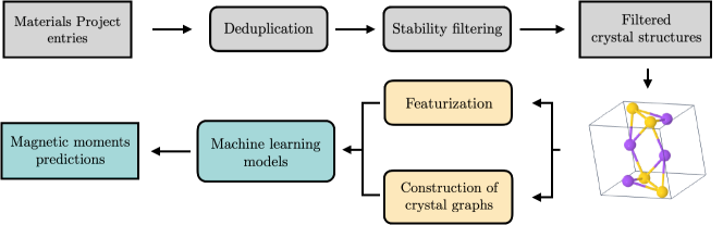
Figure 1: Data-flow for model training, including cleaning, preprocessing, and prediction steps.

II Datasets

We first discuss the Material’s Project database that was used to train the models and then the ICSD database of materials that we use to make predictions.

II.1 Materials Project

The training data used in this work comes from the Materials Project dataset (V2020.06) [8]. It is one of the largest datasets obtained from high-throughput DFT calculations and has become standard in machine learning based materials studies.

Materials Project comprises stochiometric crystalline materials, and provides their chemical composition, relaxed structures and a number of properties such as the formation energy, the energy above hull, the band structure and the spontaneous unit cell magnetization. To our knowledge, this last property in Materials Project has not been used yet for machine learning applications. Our first objective is to determine whether or not the magnetization is a property that can be modeled properly with machine learning algorithms.

We note that all the calculations are initialized in the ferromagnetic configuration. Antiferromagnetic configurations can be reached in the crystal relaxation stage. However, it has been shown that this method favours ferromagnetic configurations, even when low-spin antiferromagnetic or ferrimagnetic configurations could have lower energies [25]. In 2019, a new workflow was introduced as an effort to include appropriate antiferromagnetic ground states and counter the ferromagnetic bias [25]. At this time, new ground-state calculations using this workflow were performed for about $520$ materials, less than 2% of the Materials Project dataset.

The most difficult materials to simulate with DFT calculations are the ones in which electronic correlations are strong [26]. This is most notable in materials that contain $d$ or $f$ valence electrons, like the transition metals and the rare earths. These electrons are also the ones that participate in the magnetic properties. In the Materials Project dataset, all calculations on oxides containing Co, Cr, Fe, Mn, Mo, Ni, V and W atoms are performed with the GGA+U scheme that aims to better represent the electronic correlations. We still note that the magnetic ground state can be significantly influenced by the effect of electron-electron interactions beyond the GGA+U approximation.

We filter the entries of the Materials Project dataset to create our training set. This is because the predictions of our machine learning models can only come from the identification of patterns within this dataset. It is therefore crucial to identify biases and potential obstacles to generalization in this training distribution [27]. We first remove duplicates from the dataset. Indeed, in the dataset there is an entry for each calculation, and not each material, which results in having entries with only marginal structural differences. We use a simple heuristic to remove duplicates from the dataset. Two materials are considered similar if they share the same unit cell composition and space group. This criterion is conservative, but computationally tractable and allows to effectively remove duplicates.

Another important source of errors comes from the fact that DFT can relax to unstable, high-energy structures. Not only these materials cannot be synthesized and will drive the distribution away from materials of interest, but they will also tend to exhibit atypical features that could confuse training. We thus choose to filter these materials out of the dataset based on their energy above hull computed by DFT. The energy above hull gives the energy of decomposition of a material into a set of stable materials containing all the chemical elements of the original material and whose total formation energy is smaller. As shown in Figure 2, the distribution of energies above hull is highly skewed towards small values for entries that also appear in ICSD (i.e. materials that have been synthesized). We choose heuristically the value of $E=0.1\text{eV}/\text{atom}$ as a threshold for stability. This results in keeping $69\%$ of the materials in the dataset (Figure 3). The total curated dataset leaves us with 78 462 materials.

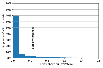
Figure 2: Distribution of the energy above hull attribute in the Materials Project dataset for the subset of entries that are also in the ICSD dataset.

The Materials Project dataset is not specifically focused on magnetic materials and includes non-magnetic (which includes paramagnetic since only spontaneous magnetization is reported), ferromagnetic and antiferromagnetic materials. For our goal of predicting magnetization, having both non-magnetic and magnetic materials is a desirable property: we want the model to identify the factors promoting strong magnetization as well as those inhibiting it. Figure 3 shows that the proportion of magnetic materials increases with the energy above hull, so eliminating large energy above hull material helps fill this criterion of having a more balanced proportion of magnetic and non-magnetic materials.

The number of materials for each magnetic order is indicated in Figure 4 for all materials and for those that are stable according to our criterion. We note that the procedure of filtering out unstable structures helps to alleviate the ferromagnetic bias of DFT. Figure 4 further shows that the eliminated materials are more ferromagnetic and ferrimagnetic; the proportion of antiferromagnetic materials slightly increases after filtering.

Further details on Materials Project are provided in Appendix A of the Suplementary Material.

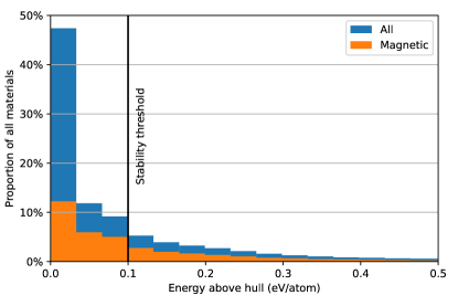
Figure 3: Distribution of the energy above hull attribute in the Materials Project dataset.

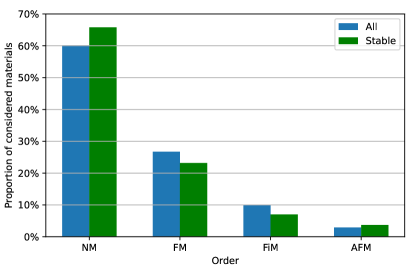
Figure 4: Distribution of magnetic orders in the Materials Project dataset. NM stands for non-magnetic, FM for ferromagnetic, FiM for ferrimagnetic and AFM for antiferromagnetic.

II.2 ICSD

Having trained models on the Materials Project, our second objective is to identify high magnetization candidates that can readily be synthesized. We use data from the Inorganic Crystal Structures Database (ICSD) to perform this task. It is currently the largest database of experimentally identified crystalline materials.

ISCD data is obtained directly from scientific publications. It includes chemical composition as well as crystal structure data for all of its entries.

Unlike the Materials Project, ICSD includes non-stochiometric materials. Since our training distribution did not include such materials, we expect that our models will have difficulty generalizing to these materials and we have thus removed these entries from the inference dataset. In addition, it is crucial to take into account that the Materials Project and ICSD datasets are not independent. The crystal structures of the entries in Materials project are computed starting from ICSD entries. Though some of the structures change significantly through the relaxation process, many of them remain sufficiently similar to the ICSD starting point to be considered as common entries between the two datasets. We have identified the common entries in both datasets and found that out of the $110~{}870$ entries in ICSD that are stochiometric and compatible with the methods, $23~{}311$ materials did not have matching identifiers or formulas. Inference of magnetization was therefore perfomed on this subset.

III Methods

Once trained, machine learning algorithms have the crucial advantage of producing predictions orders of magnitude faster than simulation methods like DFT. We can thus use them to efficiently screen candidate materials in a large database. The setup is that of a supervised learning task: given a training set of materials with features $\mathbf{X}$ and known ground-truth targets $\mathbf{Y}$, the algorithm is tasked to learn a prediction function $\mathbf{\hat{Y}}=f_{\pmb{\theta}}\left(\mathbf{X}\right)$. Training parameters $\pmb{\theta}$ are optimized to minimize a loss function $\mathcal{L}\left(\mathbf{Y},\mathbf{\hat{Y}}\right)$.

In the following subsections, we describe the learning algorithms we have used. Hyperparameters are given in Appendix B of the Supplementary Material. Aside from the more complex machine learning methods discussed in this paper, we also used the linear model [28]. The linear model is trained using the same descriptor space as the random forest. Since the linear model assumes a simple relation between each descriptor and the target, it is not expected to be accurate. Therefore, it establishes a performance baseline against which more elaborate methods will be compared. Figure 5 summarizes schematically the methods that we use. We explain each of them in more detail below.

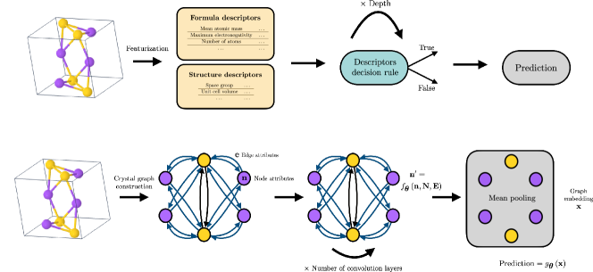
Figure 5: Methods used for property prediction. Top panel: Illustration of a decision tree. First, descriptors are computed from the chemical formula and the structural properties. A series of decisions are then taken using the descriptors. After a number of decisions, the final prediction is made. Bottom panel: Illustration of a GNN. A graph is built from the crystal unit cell. Each atom is mapped to a node and an edge is drawn between two nodes if they share a Voronoi face. Both nodes and edges have associated embedding vectors. The graph then goes through a series of graph convolution operations (defined differently for each method) parameterized by the neural network $f_{\pmb{\theta}}$. Finally, the features of all the nodes are averaged and the resulting vector goes through a multilayer perceptron $g_{\pmb{\theta}}$ that outputs the prediction.

III.1 Random Forests

The random forest [29] is a tree-based machine learning algorithm that has been widely used for materials property prediction [4, 5, 6]. Random forests have yielded encouraging results for similar material design tasks, for example finding superconductors [30, 31]. At the root of any tree-based method lies the decision tree, which carries out consecutive binary splits in the descriptor space of the data (see Figure 5). Single decision trees, however, have the major drawback of frequently overfitting the training data. Random forests go around this problem by averaging the predictions of multiple decision trees. Each tree is built differently to ensure that there is some variance in the generated forest. Randomness is implemented by choosing a subset of the descriptors to be available to the usual tree algorithm every time the algorithm makes a split. The subset is different for every split. The number of descriptors in the subset is a hyperparameter called “Available features per split”. The use of random forests is motivated in our case by their relative simplicity and efficiency [32]. We use scikit-learn’s [28] implementation of the random forest methods.

The model takes descriptors handcrafted for each sample material as input. The algorithm achieves much better performance if descriptors are well adapted to the task. The properties found in both Materials Project and ICSD, such as density and crystal structure, can be employed in our case. Inspired by other works [31, 30], most of the descriptors are obtained from the chemical formula of the materials: starting from atomic properties, such as the ground-state magnetic moment, the electronegativity, the atomic mass or the ground state d-shell electrons, we compute the mean value, the maximum value or the standard deviation of each of these properties to form descriptors. A number of descriptors are also obtained from the crystal structure, for example the number of sites in the unit cell or bond lengths. We design more than 400 descriptors in this way for each material encountered. Appendix D of the Supplementary Material gives details on descriptor design and provides an exhaustive list of all descriptors available to our random forest model.

Using this large descriptor space would lead to overfitting. Hence we identify a subset of descriptors that, in addition to yielding better predictions, comes with the added benefit of giving more interpretability to the model. Because of the large number of descriptors and material entries, forward and backward descriptor selection methods one would typically use for this task require an unreasonable amount of computational resources and time. We therefore design a descriptor selection scheme that mixes both forward and backward descriptor selection in order to efficiently find which descriptors are relevant for the task (details in Appendix E of the Supplementary Material).

III.2 Graph Neural Networks

Graph neural networks (GNNs) are deep learning architectures that are widely used for molecular-property prediction and generation [33, 34]. Their use in the context of materials is however recent. The main advantage of using GNNs for materials property prediction compared to other machine learning methods is that they only take as input a graph encoding of the material that naturally encodes structure information. The need for using handcrafted features is eliminated, as the deep model acts as a feature extractor. This ability to learn a representation adapted to the task at hand from the raw data has been key to the success of deep learning in a variety of domains. However, it is essential to note that this additional expressivity (the complexity and diversity of prediction functions that can be learned) comes at the cost of interpretability. It is notoriously difficult to know how a neural network selects specific features for predictions [35]. For this reason, we deem more appropriate to use neural networks in conjunction with random forests, a method that allows explicit descriptor construction and selection.

Here we use two architectures, CGCNN [12] and MEGNet [13] that have been chosen for their performance on other properties of the Materials Project dataset as well as their good training speed. For each material, the crystal unit cell is mapped to a sparse graph. This is done by associating each atom to a node and linking two nodes if they share a Voronoi face and are within a cutoff distance of 5 angstroms. Edges are also added if a face is shared with an atom outside the unit cell to enforce periodic boundary conditions. Around 5% of structures resulted in disconnected graphs and were discarded. When building the graphs, node features are added by taking one-hot encodings of the corresponding atomic type. This allows to capture all the information on atoms composing the unit cell. An encoding based on the distance for edges is used as well. Taking inspiration from Schnet [14], this distance is expanded on a Gaussian basis of functions, with details specified in Appendix B of the Supplementary Material.

Each architecture takes these labeled graphs as input and applies successive graph convolution layers to them (see Figure 5). These convolution operations consist of each node aggregating the features of its neighbors using a learned function. The main difference between the two models revolves around the design of these layers, which is detailed in the original papers. After a number of passes in convolution layers, node and edge representations are pooled and sent to a regressor multilayer perceptron that outputs the final prediction. For each architecture, we use the original hyperparameters with a few modifications detailed in Appendix B in the Supplementary Material [36]. Training is performed using stochastic gradient descent with the adam optimizer [37] as well as a learning rate scheduler.

III.3 Training and inference

We first train a model for each method on the Materials Project dataset. Training is performed by minimizing the mean squared error (MSE) of the predicted magnetization per atom with the Materials Project target

$$\mathcal{L}_{\text{MSE}}=\frac{1}{N}\norm{\mathbf{Y}-\mathbf{\hat{Y}}}_{2}^{2},$$ (1)

where $N$ is the size of the dataset. We also report the mean absolute error (MAE) between predicted magnetization and ground-truth values

$$\mathcal{L}_{\text{MAE}}=\frac{1}{N}\norm{\mathbf{Y}-\mathbf{\hat{Y}}}_{1}.$$ (2)

The Materials Project dataset is split into a training set comprising 80% of the data, a validation set of 10% and a test set of 10%. We compare the performance on the test of each method in Table 2. We also train models to predict the formation energy given in Materials Project. Since results on this task are obtained in the original implementations of CGCNN and MEGNet, this allows us to verify that our implementations of the models perform as well as expected.

Inference is performed using the trained model on the ICSD database. As explained above, non-stochiometric (doped) materials are eliminated since they are absent from the training set. In addition, a small fraction of the entries had incomplete crystal structure information and had to be discarded when using GNNs.

IV Results

We start by comparing the behaviour of the various methods for the prediction of the magnetization. Then, we give the predictions for magnetic moments of compounds in the ICSD dataset. We also discuss the importance of the random forest descriptors in Appendix F of the Supplementary Material.

IV.1 Evaluation of methods

We first look at the task of predicting formation energy used as a benchmark for GNN methods. We find that our models perform on par or better than the original implementations. The difference can be attributed to the fact that we use a different version of the Materials Project dataset as well as different training, validation and test set splits. Our hyperparameters are also slightly different, as detailed in Appendix B of the Supplementary Material [36]. We see that neural networks outperform random forests (Table 1) by a significant margin.

Then, we evaluate the different models on the magnetic moment prediction task on the Materials Project dataset. Results are shown on Table 2. As expected, all models outperform the baseline linear model. We find that both neural network architectures perform worse on this task than random forests. This is in strong contrast with the evaluation of prediction accuracy of formation energy. Thus, the common assumption that deep models should perform better than models based on handcrafted descriptors does not hold for the task of predicting the magnetic moment.

The difference between magnetization and formation energy results may be understood by the fact that random forests may handle imbalance in prediction labels better than neural networks. In our case, the imbalance is caused by the bimodal distribution of magnetization values, with one mode associated with non-magnetic and antiferromagnetic materials and the other with ferromagnetic and ferrimagnetic materials. These modes have significantly different weights in the distribution as shown in Figure 4. It is well known that neural networks are difficult to train on imbalanced data [38]. Deep models also show a stronger tendency to overfit training data which can explain that they compare worse on MSE than MAE. This is also confirmed by the MSE on the training set at Table VII (Appendix C of the Supplementary Material), which is one order of magnitude smaller for neural networks than for random forests.

Finally, all methods show only a smaller improvement in performance with respect to the linear model compared to the improvement on formation energy prediction. The reasons for this difficulty of predicting magnetization with more elaborate machine learning are unclear. One could argue that this could be due to the biased distribution of magnetization data in Materials Project. This is however not an entirely satisfying explanation because the test distribution is just as biased as the training distribution is. Our results instead suggest that magnetization is an intrinsically more challenging property to predict than formation energy. Better predictions could then be obtained either by incorporating more physics-based biases into the models or by accumulating more data.

Model	MAE ($eV/$atom)	MSE ($eV/$atom)
CGCNN (Original)	0.039	-
MEGNet (Original)	0.028	-
Linear Model	0.302	0.169
Random Forest	0.100	0.038
CGCNN (Ours)	0.023	0.003
MEGNet (Ours)	0.031	0.004

Table 1: Performance on the test set of the various models on prediction of the formation energy per atom using the Materials Project dataset.

Model	MAE ($\mu_{B}/$atom)	MSE ($\mu_{B}/$atom)
Linear	0.100	0.030
Random Forest	0.043	0.015
CGCNN	0.052	0.026
MEGNet	0.052	0.026

Table 2: Performance on the test set of the various models on prediction of the magnetic moment per atom using the Materials Project dataset.

IV.2 Predictions on ICSD

We now apply the trained random forests, CGCNN and MEGNet models on the ICSD dataset. We first start with the disclaimer that the predictions shown below are limited in two ways: (1) by the ferromagnetic bias of the Materials project dataset and (2) by the difficulty of predicting the magnetic moment, as shown in the previous subsection. We use the median and standard deviation of the results from the three models to estimate the magnetization and the error. In Figure 6, we illustrate the distribution of the predicted magnetic moments obtained from our three machine learning models. Despite the ferromagnetic bias present in the Materials Project dataset, we note all three models predict a majority of materials with little to no magnetization. More precisely, CGCNN, the random forests and MEGNet predict that $45$%, $47$% and $48$% of the materials have a magnetic moment smaller than $0.5\mu_{B}$/atom respectively. In Appendix G of the Supplementary Material, we show an extended analysis of the predictions on ICSD.

Figure 6: Distribution of the predicted magnetic moment for the three models: random forests (RF), CGCNN and MEGNet. Top panel shows the results in units of the Bohr magneton per atom (bin size is one Bohr magneton), bottom panel in units of magnetization per kg.

To better understand the accuracy of our predictions, we sort the results in decreasing order of the predicted magnetization per kilogram. Then, we focus on the first and last $150$ materials with the highest and lowest predicted magnetic moment per mass unit from this list. We were left with a total of about $120$ materials after removing duplicate entries (about $60$ materials with a high magnetic moment and $60$ with a zero magnetic moment). To gain an insight on the accuracy of our model, we compare the predicted magnetic properties of these materials to available experimental measurements and report our findings in Table 3. Notably, we were unable to find experimental reports on the magnetic properties of about $30$ of the materials that were predicted as having a high magnetic moment, indicating that our models could indeed be used for the discovery of new magnetic materials. We report our predictions for the magnetic moment of $15$ of these materials in Table 4. We note that all of these materials include magnetic rare-earths or magnetic transition metals. It is hence plausible that they are indeed ferromagnets with a large magnetic moment.

Coming back to Table 3, we first comment on the results for the materials with high predicted magnetic moments. We find that $17$ ($53$%) materials from this list are actually reported as ferromagnetic, or ferrimagnetic with a high magnetic moment per mass unit. The remaining materials, accounting for $47$% of this sample, are found to be mostly antiferromagnetic. This analysis of a subset of our predictions highlights the challenge in predicting the magnetization from models trained of the Materials Project dataset. The ferromagnetic bias in the training set may explain the discrepancy between the predicted ferromagnetic orders and the actual non-ferromagnetic orders observed experimentally. This emphasizes that the discrepancies between high-throughput DFT calculations and experiments can mean that the high performance of a model trained on a DFT dataset does not necessarily translate to accurate predictions when it is applied to an experimental database. We note that this conclusion applies to other predictions, not only to the prediction of the magnetic properties because the magnetic order impacts all the ground-state properties obtained through a DFT calculations.

The comparison of our predictions for small magnetic moments to available experimental data enables a better understanding of the predictive power of our models. Indeed, for these materials, we find that only $3$ materials ($9$%) from this sample are experimentally found to be ferromagnetic or ferrimagnetic, with the remaining $29$ being antiferromagnetic, non-magnetic, paramagnetic, or diamagnetic, all of which are orders with zero (or negligible) net magnetic moment. Hence, as noted before from Figure 6, the ferromagnetic bias present in the training dataset does not preclude the models from accurately predict small magnetic moments.

Magnetic order reported from experiments	Number of materials (highest magnetic moments)	Number of materials (lowest magnetic moments)
FM/FiM	$17$ ($53$%) [19, 39, 40, 41, 42, 43, 44, 45, 46, 47, 48, 49, 50, 51, 52, 53, 54]	$3$ ($9$%)[55, 56, 57]
AFM	$12$ ($38$%) [58, 59, 60, 61, 62, 52, 63, 64, 65, 66, 67, 68]	$7$ ($22$%) [69, 70, 71, 72, 73, 74, 75]
NM/PM	$2$ ($6$%) [76, 77]	$11$ ($34$%)[78, 79, 80, 81, 82, 83, 84, 85, 86]
DM	$0$ ($0$%)	$10$ ($31$%)[78, 87, 88, 89, 90]
Other	$1$ ($3$%)[91]	$1$ ($3$%)[92]

Table 3: Distribution of the magnetic orders reported experimentally for $64$ materials present in our predictions on ICSD. Middle (right) column lists the results for the $32$ materials with the highest (lowest) median magnetic moment per kilogram predicted by our models for which we could find experimental data.

Chemical formula	Moment per mass ($\mathrm{J}\mathrm{/}\mathrm{(}\mathrm{T}\times\mathrm{k}\mathrm{g}\mathrm{)}$	Rare earths
Fe9O	240 ±40	No
(Mn2O3)3MnSiO3	230 ±50	No
EuFe2	220 ±60	Yes
EuOF	220 ±20	Yes
Eu2Cu	220 ±40	Yes
Mn6O(VO4)3(OH)	220 ±80	No
EuH	220 ±90	Yes
Fe8C2	210 ±20	No
Fe8N2	200 ±30	No
GdAl	200 ±20	Yes
Eu(CN2)	200 ±60	Yes
Mn8Si6O24ClH9	200 ±60	No
Gd6Co2Al	200 ±50	Yes
Mn8O10Cl3	200 ±40	No
EuBeGd2O5	200 ±80	Yes

Table 4: Predictions of the largest magnetic moments per mass on the ICSD database for which no magnetic order reported from experiments could be found. Median values and standard deviations of the predictions of random forests, CGCNN and MEGNet are shown.

With regards to magnetic refrigeration, the rotating magnetocaloric effect is a promising recent research direction [93, 94, 95, 96, 97]. While the traditional magnetocaloric effect is due to the change in magnetization of a material under the successive application and removal of an external magnetic field, the rotating magnetocaloric effect is due to a strong magnetic anisotropy. In such anisotropic materials, the magnetization is locked in a particular crystal direction (the so-called “easy-axis”). In that case, a magnetocaloric effect is seen when the material is rotated in a fixed external magnetic field. Materials that exhibit this rotating magnetocaloric effect must have a strong spin-orbit coupling, which is usually associated to elements with a large atomic number. The materials we show in Table 4 that include Eu, Gd and In elements could potentially satisfy this requirement.

V Conclusion

To identify materials with a large magnetic moment per kilogram, we have trained random forests and two state-of-the-art deep-learning graph convolutional algorithms, CGCNN and MEGNet, on the Materials Project dataset. Since the discovery of large magnetic moments materials could lead to breakthroughs in magnetocaloric refrigeration, we choose this application as a use case. Magnetic properties in the training set are computed using DFT methods. The three machine-learning methods show comparable accuracy on the test sets. Differences in estimates for the mean average error and mean squared error suggest that the predicted magnetic moment per atom is accurate to better than 0.05 Bohr magneton per atom.

We used the trained models to search for candidate materials with large magnetic moments per kilogram in the ICSD database. That database contains materials that have been synthesized. Table 4 lists the most promising materials. These deserve experimental attention. Our analysis also highlights some of the limitations of working with magnetic properties in the Materials Project. In particular, the ferromagnetic bias affects the screening capability of models trained on this dataset. In the few cases where we could compare our predictions for ferromagnetic materials with experiment, we found that materials were indeed ferromagnetic 50% of the time. Since the rate of false negatives is low, we believe our model does not leave out many materials that are ferromagnetic. Finally, we have shown that magnetization may be intrinsically more difficult to predict than other properties. These findings provide strong arguments to motivate building a large database dedicated to magnetic properties of materials.

Data Availability

Data from the Materials Project dataset is freely available using their API. Documentation for this API is available at https://docs.materialsproject.org/open-apis/the-materials-api/. ICSD is under a proprietary license.

Code Availability

Code for the machine learning models is available from the corresponding author upon reasonable request.

Author Contributions

All authors contributed to designing the study and analyzing results. S.-O.K. wrote the code for the deep learning models. B.G.-P. and M.-A. G. wrote the code for random forests models. S.-O.K. and S.V. analyzed the datasets. S.-O.K., B.G.-P, M.-A.G., A.-M.S.T. and C. G.-N. wrote the paper. A.-M.S.T, S.V. and C.G.-N. provided supervision for the project.

Competing Interests

The authors declare no competing interests.

Appendix A Additional details on Materials Project

The Materials Project dataset is constructed using the Vienna Ab Initio Simulation Package (VASP) software [98] and the GGA functional. The calculations are done using the projector augmented wave pseudopotentials implemented in VASP. This method has the advantage of reducing computation time while retaining precision [99]. The initial crystal structures used as input for the calculations are obtained from the Inorganic Crystal Structure Database (ICSD), which we describe below. The calculations then allow for structure relaxation. All calculations are performed at $T=0$, meaning that the dataset should contain the ground state properties of materials. No spin-orbit coupling effects are included.

Figure 7 shows the distribution of elements in the Materials project dataset, blue indicating the proportion for all materials, and orange the proportion for the subset of magnetic materials. In the latter category, it is not surprising to find transition metals. Oxygen is often present in magnetic materials probably because of the prevalence of perovskite structures that make up 93% of the lower earth mantle’s mass. Surprisingly, Li is also often present in magnetic materials, which may this time reflect the interest of researchers in Li containing materials because of the technological importance of batteries.

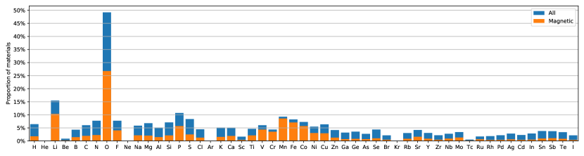
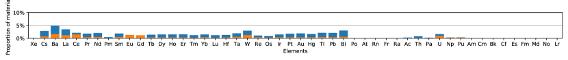
Figure 7: Histogram of entries in the Materials Project dataset categorized by the presence (irrespective of stochiometry) of a chemical specie. Blue denotes the distribution over all materials and orange over the subset of magnetic materials.

Appendix B Hyperparameters

For random forests, tuning each hyperparameter individually and in sequence prevents one from detecting possible relations between parameters. Therefore, the ultimate set of hyperparameters was found using random search.

Hyperparameter	Value
Number of descriptors	98
Bootstrap	None
Available features per split	32.5%
Minimum samples for a split	4
Minimum samples per leaf	2
Minimum depth	None

Table 5: Value of hyperparameters used for the random forest.

For neural network methods, we used the same hyperparameters for CGCNN and MEGNet for convenience reasons as well as to avoid excessive hyperparameter tuning. General hyperparameters were optimized through grid search. Other values were selected in accordance with the original architectures or by convenience given the available hardware.

	Hyperparameter	Value
General	Starting learning rate	0.001
	Patience	25
	Learning rate factor	0.5
	Batch size	1024
CGCNN	Site embedding size	100
	Bond embedding size	20
	Bond Gaussian basis size	10
	Maximum bond distance	5.2
	Hidden layer size	100
	Number of convolution layers	2
	Number of output layers	3
MEGNet	Site embedding size	36
	State embedding size	36
	Bond embedding size	36
	Bond Gaussian basis size	100
	Maximum bond distance	5.2
	Number of MEGNet layers	3
	MEGNet layer hidden size	64
	Number of output layers	3
	Output layer 1 hidden size	32
	Output layer 2 hidden size	16

Table 6: Value of hyperparameters used for neural network models.

Appendix C Training set metrics

In Table 7, we report the MSE on the training set for the different method. Small values for the loss function on the training set compared to the test set is evidence of overfitting.

Model	MSE ($\mu_{B}/$atom)
Random Forest	0.015
CGCNN	0.0010
MEGNet	0.0014

Table 7: Performance on the training set of the various models on prediction of the magnetic moment per atom using the Materials Project dataset.

Appendix D Random Forest Descriptors

Most the descriptors designed for the random forest method are built from the chemical formula of the materials only. Given a material, each atom in the chemical formula have properties specific to themselves and independent of the material. We call these properties atomic properties. A list of all atomic properties is given in Table 8. Some of these properties, such as the atomic number, the atomic mass or the valence electrons, are specific to the isolated atom, while other properties, such as the cohesive energy, the density or the melting temperature, are specific to pure materials made of this kind of atom.

Atomic properties
Atomic number	Mendeleev number
Column	Row
Ground state mag. moment	Mass
Electronegativity	First ionization energy
Covalent radius	Cohesive energy
Electron affinity	Electron binding energy
Polarizability	Density
Boiling temperature	Melting temperature
Volume per atom ($\sqrt[3]{density}$)	Atomic volume (mendeleev)
Valence electrons (s shell)	Unfilled electrons (s shell)
Valence electrons (p shell)	Unfilled electrons (p shell)
Valence electrons (d shell)	Unfilled electrons (d shell)
Valence electrons (f shell)	Unfilled electrons (f shell)
Unfilled electrons (d & f shells)	Valence electrons (Magpie)
Valence electrons (iMat)	Valence electrons (Wiki.)
Multiplicity in chemical formula

Table 8: List of atomic properties. The valence electrons atomic property differed from one source to another (iMat[31], Magpie[100] and Wikipedia[101]). All three were used. Given a chemical formula A_xB_yC_z, the multiplicity in the chemical formula atomic property is $x$ for atom species A, $y$ for atom species B, and $z$ for atom species C.

Then, different operations on these properties can be applied to each chemical formula to build scalar descriptors. All operations used in our method are shown in Table 9. Thus, given 14 operations and 31 atomic properties, $14\times 31=434$ descriptors can be built for each material.

Operations
Maximum
Minimum
Maximum difference
Minimum difference
Weighed average
Standard deviation
Average among magnetic atoms (L1, L2)
Weighed average among magnetic atoms (L1, L2, L3)
Maximum among magnetic atoms (L1)
Minimum among magnetic atoms (L1)
Standard deviation among magnetic atoms (L2)

Table 9: List of operations that can be associated with each atomic property of Table 8 to yield 434 different descriptors. There are two different averages used, average and weighed average. The weighed average is an average that accounts for the occurrence of each atom in the chemical formula, while the average computes the average between each atomic species in the chemical formula, independently of how many of each atom there is in the chemical formula.

Below are the three subsets of elements, L1, L2, and L3 that are involved in some of the descriptors in the table above. In the computation of these descriptors, all elements that are not part of the list specified in parenthesis are attributed a weight zero. These lists help build descriptors that characterise the atoms that are more likely to cause magnetism in a material. Whether an element will induce magnetism in a material is highly dependent on the crystal structure. These lists are thus heuristic. The first list (L1) is the most general. It contains all elements for which one or more of its oxidation states allow magnetism. However, after analyzing the magnetic materials part of the Materials Project database, we notice some elements in L1 nearly never induced magnetism by themselves. In other words, the materials including these elements and no other element from L1 would rarely be magnetic. The set L2 results from the removal of these elements from L1. The set L3, which is the most uncluttered, was also obtained from L1 by removing elements that seemed to be poor inducers of magnetism.

Elements included in the set L1: Sc, Ti, V, Cr, Mn, Fe, Co, Ni, Cu, Zr, Nb, Mo, Tc, Ru, Rh, Pd, Ag, Ce, Nd, Pm, Sm, Eu, Gd, Tb, Dy, Ho, Er, Tm, Yb, W, Re, Os, Ir, Pt, Au, U, Np, Pu

Elements included in the set L2: Ti, V, Cr, Mn, Fe, Co, Ni, Cu, Nb, Mo, Tc, Ru, Rh, Pd, Ce, Eu, Gd, Tb, W, Re, Os, Ir, U, Np, Pu

Elements included in the set L3: V, Cr, Mn, Fe, Co, Ni, Cu, Ru, Ce, Eu, Gd, U, Np, Pu

Descriptors built outside of the operation $\times$ atomic property scheme are listed in Table 10. Considering that each list (L1, L2, L3), when specified, represents a different descriptor and the fact that there are 7 different crystal systems, we see that there are 29 other descriptors, and 463 descriptors in total.

Other descriptors
Rate of mag. atoms (L1, L2)
Number of species
Number of different mag. atoms (L1)
Fraction of s shell valence electrons
Fraction of p shell valence electrons
Fraction of d shell valence electrons
Fraction of f shell valence electrons
Crystal system (one-hot encoding)
Material density
Number of sites
Magnetic atoms avg. bond length (L1, L2, L3)
Magnetic atoms avg. bond angle (L1, L2, L3)
Magnetic atoms std. bond length (L1, L2, L3)
Magnetic atoms std. bond angle (L1, L2, L3)

Table 10: Descriptors that differ from the operation $\times$ atomic property building scheme. The last 7 descriptors of the table are the only ones that come from the actual crystal structure of the materials. Only first neighbors are considered in the computation of the average bond length and average bond angle descriptors.

Appendix E Random Forest Descriptor Selection

Our feature selection method converges iteratively towards the final set of descriptors. The scheme works by chunking the training data and descriptor space into smaller sets on which forward and backward feature selection methods are then performed.

Figure 8: Schematic view of one step of the feature selection scheme.

An example is the best way to illustrate the feature selection method. Suppose one wants to build a random forest regressor from a 100,000-entries training set using only a handful of features from a very large descriptor space. Performing a regular forward or backward feature selection on the whole training set to obtain an optimal set of descriptors would require an unreasonable amount of computational resources and time. To reduce the computational time, one splits its training dataset in 25 equal parts, which results in chunks of data of 4000 materials each. One then performs a forward and a backward feature selection on every chunk of data for a total of 50 calculations. Since the dataset size is much smaller, the computation time is significantly reduced. One then counts the occurrence of each descriptor in the final set of 10 most important descriptors that are selected by each of the 50 calculations and removes half of the descriptors based on their low or null occurrence. A schematic view of this process is shown in Figure 8. The same operation can be repeated on the new descriptor space to remove even more descriptors and get closer to an optimal final set of descriptors. However, this time, the dataset can be split in fewer chunks since the are less descriptors to choose from. Note that the choices made in this example, such as the number of chunks and the number of descriptors removed at each step, are arbitrary and chosen for convenience.

Out of the 463 available descriptors obtained following the method described in Appendix D, this descriptor selection scheme allowed us to select a subset of 98 relevant descriptors. Some of the selected descriptors are still more relevant for the task than others. The importance of each descriptor in determining the magnetic moment is estimated from the mean impurity decrease it provides when selected for a split. The results are shown in Appendix F.

The first 16 descriptor account for nearly 75% of the total importance score. However, the remaining 82 descriptors still play an important role in the decision trees. These descriptors allow finer cuts in the data that are crucial to the algorithm performance. In order to test the relevance of these least important descriptors, we ran the random forest algorithm using only the 16 most important descriptors according to Table 11, yielding an MAE of 0.072 and an MSE of 0.029, both substantially larger than when the 98 descriptors are used (0.043 and 0.015 respectively in Table 2).

The descriptor with the highest importance ($22.9\%$) is the “weighted average of f-shell valence electrons (L3)”. This predictor contains information about whether the material contains atoms from L3 that are part of the lanthanide or actinide family or not. The next four most important descriptors are all based on the “ground state atomic magnetic moment” atomic property. The relevance of these predictors is not surprising. Notice that as a result of the operation $\times$ atomic property building scheme, the “Max. at. magnetic moment” and “Max. among mag. at. magnetic moment” are identical.

Appendix F Random Forest Descriptor Importance

We use the descriptor importance score [102] available in the scikit-learn. The method works by computing how on average each descriptor decreases the impurity when used in a split. The mean impurity decrease is computed for all descriptors and normalized over the entire descriptor set to give the importance score displayed in Table 11.

Descriptor	Importance (%)	Descriptor	Importance (%)
Weighted avg. (L3) f shell valence el.	22.920	Max. among mag at. boiling T	0.371
Max. at. magnetic moment	10.397	Weighted avg. (L1) at. column	0.336
Weighted avg. (L3) at. magnetic moment	8.172	Std. at. covalent radius	0.328
Max. among mag at. magnetic moment	6.305	Std. at. valence el. (Wiki.)	0.322
Avg. among mag. (L2) at. magnetic moment	4.835	Min. among mag el. binding energy	0.315
Weighted avg. (L3) at. volume (mendeleev)	3.032	Weighted avg. (L3) mendeleev number	0.304
Weighted avg. (L3) at. valence el. (iMat)	2.964	Avg. among mag. (L2) at. valence el. (iMat)	0.286
Weighted avg. (L3) at. d+f unfilled el.	2.656	Weighted avg. at. valence el. (Magpie)	0.285
Weighted avg. (L3) at. volume	2.479	Avg. among mag. (L2) at. density	0.254
Weighted avg. (L3) at. polarizability	2.289	Weighted avg. at. valence el. (Wiki.)	0.250
Min. among mag at. electron affinity	1.862	Weighted avg. at. p valence el.	0.237
Avg. among mag. (L2) at. electron affinity	1.744	Std. multiplicity in the chemical formula	0.236
Weighted avg. (L3) f shell unfilled el.	1.376	Min. among mag Z	0.225
Weighted avg. (L3) at. unfilled el.	1.374	Avg. among mag. (L2) at. electronegativity	0.212
Avg. among mag. (L2) at. boiling T	1.179	Weighted avg. multiplicity in the chemical formula	0.204
Weighted avg. (L3) multiplicity in the chemical formula	1.154	Max. among mag at. melting T	0.184
Weighted avg. (L3) at. valence el. (Magpie)	0.900	Max. at. volume	0.181
Weighted avg. (L3) at. valence el. (Wiki.)	0.865	Avg. among mag. (L2) at. column	0.173
Max. at. cohesive energy	0.840	Min. at. cohesive energy	0.170
Weighted avg. (L2) f shell valence el.	0.738	Max. f shell valence el.	0.162
Std. at. electron affinity	0.724	Max. among mag multiplicity in the chemical formula	0.146
Mag. avg. bond length (L3)	0.694	Min. among mag at. valence el. (Magpie)	0.142
Weighted avg. (L3) at. mass	0.691	Min. among mag at. mass	0.137
Weighted avg. (L2) at. magnetic moment	0.687	Max. at. melting T	0.131
Weighted avg. at. cohesive energy	0.648	Max. difference multiplicity in the chemical formula	0.119
Mag. avg. bond length (L2)	0.647	Max. at. polarizability	0.112
Nb. sites	0.634	Max. among mag mendeleev number	0.110
Std. among mag f shell unfilled el.	0.565	Min. at. boiling T	0.108
Weighted avg. (L3) at. electron affinity	0.563	Max. multiplicity in the chemical formula	0.104
Mag. std. bond angle (L3)	0.537	Max. at. column	0.104
Mag. std. bond length (L3)	0.500	Max. at. p valence el. el.	0.101
Mag. avg. bond length (L1)	0.497	Max. d shell valence el.	0.086
Weighted avg. at. unfilled el.	0.484	Min. at. electronegativity	0.085
Weighted avg. f shell unfilled el.	0.474	Max. difference at. p valence el.	0.083
Weighted avg. at. electron affinity	0.468	Max. at. valence el. (iMat)	0.075
Weighted avg. at. volume	0.463	Max. at. valence el. (Wiki.)	0.066
Max. difference at. volume	0.448	Max. at. unfilled el.	0.066
Weighted avg. (L3) at. column	0.433	Min. among mag first ionization energy	0.065
Weighted avg. at. boiling T	0.431	Max. difference d shell unfilled el.	0.063
Std. at. p valence el.	0.420	Min. among mag mendeleev number	0.062
Weighted avg. (L2) multiplicity in the chemical formula	0.415	Max. among mag at. volume	0.060
Mag. std. bond angle (L2)	0.413	Max. among mag d shell valence el.	0.054
Mag. std. bond length (L2)	0.398	Max. at. d+f unfilled el.	0.049
Avg. among mag. (L2) at. volume	0.397	Max. among mag at. d+f unfilled el.	0.046
Mag. std. bond length (L1)	0.397	Avg. among mag. (L2) at. row	0.042
Weighted avg. (L1) multiplicity in the chemical formula	0.389	Min. among mag at. electronegativity	0.040
Weighted avg. at. melting T	0.386	Max. f shell unfilled el.	0.026
Min. el. binding energy	0.381	Avg. among mag. (L2) f shell unfilled el.	0.021
Weighted avg. at. density	0.375	Max. among mag f shell unfilled el.	0.020

Table 11: List of descriptors ordered by importance score

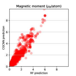
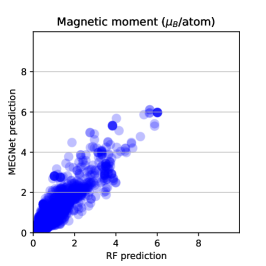
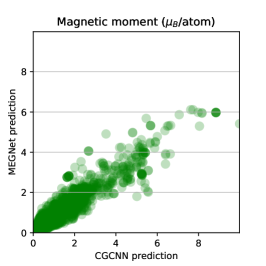
Figure 9: Scatter plots of the predicted magnetic moment per atom as a function of the machine learning models.

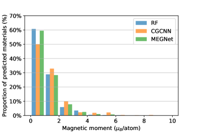
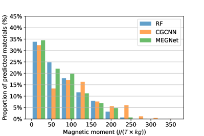
Figure 10: Histograms of the predicted magnetic moments for materials that contain at least one magnetic atom as defined by the L2 list detailed in Appendix F. Left (right) panel shows the magnetic moment per atom (kg).

Appendix G More details on the predictions on ICSD

In this Appendix, we offer more analysis of the predictions on the ICSD database. We start by illustrating the distribution of the predictions as a function of the machine learning model in Figure 9. These scatter plots yield information similar to that given in the histograms of Figure 6. A perfectly linear distribution would indicate that two methods give the exact same predictions for the same materials. The deviation to linearity observed in the plots instead show the degree of variability offered by the different methods. As anticipated from the histograms shown in Figure 6, the random forest and MEGNet predictions are closer to each other than they are to the CGCNN predictions.

Next, we produce histograms of the predicted magnetic moments per atom and per mass unit analogous to the ones shown in Figure 6, but this time we only plot the data for the materials that contain at least one magnetic element as defined in the L2 list of Appendix F. The results are shown in Figure 10. The reason we choose to illustrate the results in this way is to investigate whether or not the models simply predict high values of the magnetic moments for materials that contain magnetic atoms, which would render the predictions trivial. However, comparing Figures 10 and 6, we note that the distributions of the predicted magnetic moments for the full dataset and for the filtered one are similar. More specifically, between $35$% and $38$% of the materials containing at least one element belonging to the L2 list are predicted as having a magnetic moment smaller than $0.5\mu_{B}$/atom. These proportions are smaller than the ones for the full dataset ($45$% to $48$%). This is expected since the elements of L2 are the ones that were found to result in non-zero magnetism in the Materials Project database. However, the high proportion of small predicted magnetic moments for this subset of the ICSD database leads us to believe that the predictions we obtain are more than a trivial classification of materials containing specific elements.

References

- Liu et al. [2020] Z.-L. Liu, P. Kang, Y. Zhu, L. Liu, and H. Guo, Material informatics for layered high-tc superconductors, APL Materials 8, 061104 (2020).
- Wu et al. [2020] Y. Wu, J. Guo, R. Sun, and J. Min, Machine learning for accelerating the discovery of high-performance donor/acceptor pairs in non-fullerene organic solar cells, npj Computational Materials 6, 120 (2020).
- Ortiz et al. [2009] C. Ortiz, O. Eriksson, and M. Klintenberg, Data mining and accelerated electronic structure theory as a tool in the search for new functional materials, Computational Materials Science 44, 1042 (2009).
- Ward et al. [2016] L. Ward, A. Agrawal, A. Choudhary, and C. Wolverton, A general-purpose machine learning framework for predicting properties of inorganic materials, npj Computational Materials 2, 10.1038/npjcompumats.2016.28 (2016).
- Landrum and Genin [2003] G. A. Landrum and H. Genin, Application of machine-learning methods to solid-state chemistry: ferromagnetism in transition metal alloys, Journal of Solid State Chemistry 176, 587 (2003), special issue on The Impact of Theoretical Methods on Solid-State Chemistry.
- Rhone et al. [2020] T. D. Rhone, W. Chen, S. Desai, S. B. Torrisi, D. T. Larson, A. Yacoby, and E. Kaxiras, Data-driven studies of magnetic two-dimensional materials, Scientific Reports 10, 10.1038/s41598-020-72811-z (2020).
- Möller et al. [2018] J. J. Möller, W. Körner, G. Krugel, D. F. Urban, and C. Elsässer, Compositional optimization of hard-magnetic phases with machine-learning models, Acta Materialia 153, 53 (2018).
- Jain et al. [2013] A. Jain, S. P. Ong, G. Hautier, W. Chen, W. D. Richards, S. Dacek, S. Cholia, D. Gunter, D. Skinner, G. Ceder, and K. a. Persson, The Materials Project: A materials genome approach to accelerating materials innovation, APL Materials 1, 011002 (2013).
- Kirklin et al. [2015] S. Kirklin, J. E. Saal, B. Meredig, A. Thompson, J. W. Doak, M. Aykol, S. Rühl, and C. Wolverton, The open quantum materials database (oqmd): assessing the accuracy of dft formation energies, npj Computational Materials 1, 15010 (2015).
- Court and Cole [2020] C. J. Court and J. M. Cole, Magnetic and superconducting phase diagrams and transition temperatures predicted using text mining and machine learning, npj Computational Materials 6, 10.1038/s41524-020-0287-8 (2020).
- Curtarolo et al. [2012] S. Curtarolo, W. Setyawan, G. L. Hart, M. Jahnatek, R. V. Chepulskii, R. H. Taylor, S. Wang, J. Xue, K. Yang, O. Levy, M. J. Mehl, H. T. Stokes, D. O. Demchenko, and D. Morgan, Aflow: An automatic framework for high-throughput materials discovery, Computational Materials Science 58, 218 (2012).
- Xie and Grossman [2018] T. Xie and J. C. Grossman, Crystal graph convolutional neural networks for an accurate and interpretable prediction of material properties, Physical Review Letters 120, 10.1103/physrevlett.120.145301 (2018).
- Chen et al. [2019] C. Chen, W. Ye, Y. Zuo, C. Zheng, and S. P. Ong, Graph networks as a universal machine learning framework for molecules and crystals, Chemistry of Materials 31, 3564 (2019), https://doi.org/10.1021/acs.chemmater.9b01294 .
- Schütt et al. [2017] K. Schütt, P.-J. Kindermans, H. E. S. Felix, S. Chmiela, A. Tkatchenko, and K.-R. Müller, Schnet: A continuous-filter convolutional neural network for modeling quantum interactions, in Advances in Neural Information Processing Systems (2017) pp. 991–1001.
- Nakamura [2018] H. Nakamura, The current and future status of rare earth permanent magnets, Scripta Materialia 154, 273 (2018).
- Weiss, Pierre and Piccard, Auguste [1917] Weiss, Pierre and Piccard, Auguste, Le phénomène magnétocalorique, J. Phys. Theor. Appl. 7, 103 (1917).
- Gómez et al. [2013] J. R. Gómez, R. F. Garcia, A. D. M. Catoira, and M. R. Gómez, Magnetocaloric effect: A review of the thermodynamic cycles in magnetic refrigeration, Renewable and Sustainable Energy Reviews 17, 74 (2013).
- Smith et al. [2012] A. Smith, C. R. Bahl, R. Bjørk, K. Engelbrecht, K. K. Nielsen, and N. Pryds, Materials challenges for high performance magnetocaloric refrigeration devices, Advanced Energy Materials 2, 1288 (2012).
- Brown [1976] G. V. Brown, Magnetic heat pumping near room temperature, Journal of Applied Physics 47, 3673 (1976), https://doi.org/10.1063/1.323176 .
- Pecharsky and Gschneidner [1997] V. K. Pecharsky and K. A. Gschneidner, Jr., Giant magnetocaloric effect in , Phys. Rev. Lett. 78, 4494 (1997).
- Breiman [2001] L. Breiman, Random forests, Machine learning 45, 5 (2001).
- James et al. [2017] G. James, D. Witten, T. Hastie, and R. Tibshirani, An Introduction to Statistical Learning, 8th ed. (Springer, New York, 2017).
- Liaw and Wiener [2002] A. Liaw and M. Wiener, Classification and regression by randomforest, R news 2, 18 (2002).
- Bergerhoff et al. [1983] G. Bergerhoff, R. Hundt, R. Sievers, and I. Brown, The inorganic crystal structure data base, Journal of chemical information and computer sciences 23, 66 (1983).
- Horton et al. [2019] M. K. Horton, J. H. Montoya, M. Liu, and K. A. Persson, High-throughput prediction of the ground-state collinear magnetic order of inorganic materials using density functional theory, npj Computational Materials 5, 64 (2019).
- Pavarini [2021] E. Pavarini, Solving the strong-correlation problem in materials, La Rivista del Nuovo Cimento 10.1007/s40766-021-00025-8 (2021).
- Gudivada et al. [2017] V. Gudivada, A. Apon, and J. Ding, Data quality considerations for big data and machine learning: Going beyond data cleaning and transformations, International Journal on Advances in Software 10, 1 (2017).
- Pedregosa et al. [2011] F. Pedregosa, G. Varoquaux, A. Gramfort, V. Michel, B. Thirion, O. Grisel, M. Blondel, P. Prettenhofer, R. Weiss, V. Dubourg, J. Vanderplas, A. Passos, D. Cournapeau, M. Brucher, M. Perrot, and Édouard Duchesnay, Scikit-learn: Machine learning in python, Journal of Machine Learning Research 12, 2825 (2011).
- Tin Kam Ho [1995] Tin Kam Ho, Random decision forests, in Proceedings of 3rd International Conference on Document Analysis and Recognition, Vol. 1 (1995) pp. 278–282 vol.1.
- Stanev et al. [2018] V. Stanev, C. Oses, A. G. Kusne, E. Rodriguez, and J. Paglione, Machine learning modeling of superconducting critical temperature, npj Computational Materials 4 (2018).
- Liu et al. [2019] Z.-L. Liu, P. Kang, Y. Zhu, L. Liu, and H. Guo, Material informatics for superconductors (2019).
- Louppe [2015] G. Louppe, Understanding Random Forests: From Theory to Practice, Ph.D. thesis, University of Liège (2015).
- Duvenaud et al. [2015] D. K. Duvenaud, D. Maclaurin, J. Iparraguirre, R. Bombarell, T. Hirzel, A. Aspuru-Guzik, and R. P. Adams, Convolutional networks on graphs for learning molecular fingerprints, in Advances in neural information processing systems (2015) pp. 2224–2232.
- Gilmer et al. [2017] J. Gilmer, S. S. Schoenholz, P. F. Riley, O. Vinyals, and G. E. Dahl, Neural message passing for quantum chemistry, in Proceedings of the 34th International Conference on Machine Learning, Proceedings of Machine Learning Research, Vol. 70, edited by D. Precup and Y. W. Teh (PMLR, International Convention Centre, Sydney, Australia, 2017) pp. 1263–1272.
- Chakraborty et al. [2017] S. Chakraborty, R. Tomsett, R. Raghavendra, D. Harborne, M. Alzantot, F. Cerutti, M. Srivastava, A. Preece, S. Julier, R. M. Rao, et al., Interpretability of deep learning models: A survey of results, in 2017 IEEE smartworld, ubiquitous intelligence & computing, advanced & trusted computed, scalable computing & communications, cloud & big data computing, Internet of people and smart city innovation (smartworld/SCALCOM/UIC/ATC/CBDcom/IOP/SCI) (IEEE, 2017) pp. 1–6.
- [36] See Supplemental Material at [url] for information on the datasets used in the study, implementation of the machine learning models and additional results. Also included are references [100-104].
- Kingma and Ba [2014] D. P. Kingma and J. Ba, Adam: A method for stochastic optimization, arXiv preprint arXiv:1412.6980 (2014).
- Johnson and Khoshgoftaar [2019] J. M. Johnson and T. M. Khoshgoftaar, Survey on deep learning with class imbalance, Journal of Big Data 6, 1 (2019).
- Chen and Zhuang [2008] X. Chen and Y. H. Zhuang, Magnetocaloric effect of gd12co7, Solid State Communications 148, 322–325 (2008).
- Crangle and Goodman [1971] J. Crangle and G. M. Goodman, The magnetization of pure iron and nickel, Proceedings of the Royal Society of London. Series A, Mathematical and Physical Sciences 321, 477–491 (1971).
- Hong et al. [2005] H.-M. Hong, Y.-J. Kang, J. Kang, E.-C. Lee, Y.-H. Kim, and K. J. Chang, Effect of chemical bonding on the magnetic stability and magnetic moment in mn-based binary compounds, Physical Review B 72, 144408 (2005).
- Hong et al. [2018] K. H. Hong, A. M. Arevalo-Lopez, M. Coduri, G. M. McNally, and J. P. Attfield, Cation, magnetic, and charge ordering in mnfe3o5, Journal of Materials Chemistry C 6, 3271–3275 (2018).
- Jiang et al. [2018] L. Jiang, S. Yang, M. Zheng, H. Chen, and A. Wu, Synthesis and magnetic properties of nanocrystalline gd3fe5o12 and gdfeo3 powders prepared by sol–gel auto-combustion method, Materials Research Bulletin 104, 92–96 (2018).
- Mansmann and Wallace [1964] M. Mansmann and W. E. Wallace, Magnetic properties of gdfe2 and dyfe2, The Journal of Chemical Physics 40, 1167–1168 (1964).
- Modder et al. [1999] I. W. Modder, H. Bakker, and G. F. Zhou, Defects and magnetism in cubic gdx2 laves phase compounds, Physica B: Condensed Matter 262, 141–158 (1999).
- Rafiq et al. [2021] M. A. Rafiq, A. Javed, M. N. Rasul, M. Nadeem, F. Iqbal, and A. Hussain, Structural, electronic, magnetic and optical properties of ab2o4 (a = ge, co and b = ga, co) spinel oxides, Materials Chemistry and Physics 257, 123794 (2021).
- Tsuzuki et al. [1984] A. Tsuzuki, S. Sago, S. I. Hirano, and S. Naka, High temperature and pressure preparation and properties of iron carbides fe7c3 and fe3c, Journal of Materials Science 19, 2513–2518 (1984).
- Wakizaka et al. [2022] M. Wakizaka, W.-J. Chun, T. Imaoka, and K. Yamamoto, Synthesis and magnetic properties of sub-nanosized iron carbides on a carbon support, RSC Advances 12, 3238–3242 (2022).
- Williams et al. [2003] D. Williams, P. M. Shand, C. Stark, T. Pekarek, R. Brown, L. Yue, and D. L. Leslie-Pelecky, Curie–weiss analysis of ferromagnetic and glassy transitions in nanostructured gdal2, Journal of Applied Physics 93, 6525–6527 (2003).
- Yamamoto et al. [2020] T. Yamamoto, K. Kaminaga, D. Saito, D. Oka, and T. Fukumura, Rock salt structure gdo epitaxial thin film with a high ferromagnetic curie temperature, Applied Physics Letters 117, 052402 (2020).
- Zhao et al. [2017] N. Zhao, W. Wang, X. Lei, Z. Ye, X. Chen, H. Ding, and H. Yang, Synthesis, structure and magnetic properties of fe3n nanoparticles, Journal of Materials Science: Materials in Electronics 28, 15701–15707 (2017).
- McWhan et al. [1966] D. B. McWhan, P. C. Souers, and G. Jura, Magnetic and structural properties of europium metal and europium monoxide at high pressure, Physical Review 143, 385–389 (1966).
- Le Binh et al. [2013] D. Le Binh, B. J. Ruck, F. Natali, H. Warring, H. J. Trodahl, E.-M. Anton, C. Meyer, L. Ranno, F. Wilhelm, and A. Rogalev, Europium nitride: A novel diluted magnetic semiconductor, Physical Review Letters 111, 167206 (2013).
- Pecharsky et al. [2002] V. Pecharsky, K. Gschneidner, S. Y. Dan’kov, and A. Tishin, Magnetocaloric properties of gd3al2, in Cryocoolers 10, edited by R. G. Ross (Springer US, Boston, MA, 2002) p. 639–645.
- Anton et al. [2016] E.-M. Anton, J. F. McNulty, B. J. Ruck, M. Suzuki, M. Mizumaki, V. N. Antonov, J. W. Quilty, N. Strickland, and H. J. Trodahl, Ndn: An intrinsic ferromagnetic semiconductor, Physical Review B 93, 064431 (2016).
- Labroo and Ali [1998] S. Labroo and N. Ali, Magnetism of rare‐earth disilicides, Journal of Applied Physics 67, 4811 (1998).
- Zhong et al. [2011] X. C. Zhong, M. Zou, H. Zhang, Z. W. Liu, D. C. Zeng, K. A. Gschneidner, and V. K. Pecharsky, Crystal structure and magnetic properties of r5sn4 alloys, where r is tb, dy, ho, and er, Journal of Applied Physics 109, 07A917 (2011).
- Yakubovich et al. [2017] O. V. Yakubovich, L. V. Shvanskaya, O. V. Dimitrova, O. S. Volkova, and A. N. Vasiliev, Magnetically frustrated synthetic end member mn2(po4)oh in the triplite–triploidite family, Dalton Transactions 46, 8680–8686 (2017).
- Wada and Shiga [1994] H. Wada and M. Shiga, Antiferromagnetic properties of eual2, Physica B: Condensed Matter 193, 25–30 (1994).
- Tristan et al. [2002] N. V. Tristan, S. A. Nikitin, T. Palewski, K. Skokov, and J. Warchulska, Magnetization of a gd3ni single crystal, Journal of Alloys and Compounds 334, 40–44 (2002).
- Roger et al. [2006] J. Roger, V. Babizhetskyy, K. Hiebl, J.-F. Halet, and R. Guérin, Structural chemistry, magnetism and electrical properties of binary gd silicides and ho3si4, Journal of Alloys and Compounds 407, 25–35 (2006).
- Pollard et al. [1983] R. J. Pollard, V. H. McCann, and J. B. Ward, Magnetic structures of alpha-mns and mnse from 57fe mossbauer spectroscopy, Journal of Physics C: Solid State Physics 16, 345 (1983).
- Li et al. [2000] X. G. Li, M. Sato, S. Takahashi, K. Aoki, and T. Masumoto, Magnetic properties of gd2al compound in amorphous, crystalline and nitrided states, Journal of Magnetism and Magnetic Materials 212, 145–152 (2000).
- Carlin et al. [1980] R. L. Carlin, R. D. Chirico, K. O. Joung, G. K. Shenoy, and D. G. Westlake, Magnetic ordering in gdh3, Physics Letters A 75, 413–414 (1980).
- Kolenda et al. [1990] M. Kolenda, A. Szytula, J. Leciejewicz, A. Pawlukojc, and H. Ptasiewicz-Bak, Magnetic structure of mn3ni2si, Journal of Magnetism and Magnetic Materials 89, 26–28 (1990).
- Johnson et al. [2018] R. D. Johnson, D. D. Khalyavin, P. Manuel, L. Zhang, K. Yamaura, and A. A. Belik, Magnetic structures of the rare-earth quadruple perovskite manganites r mn 7 o 12, Physical Review B 98, 104423 (2018).
- Hémon et al. [2000] S. Hémon, R. A. Cowley, R. C. C. Ward, M. R. Wells, L. Douysset, and H. Ronnow, Magnetic structure of gd, gdh2 and ndh2 single crystal films, Journal of Physics: Condensed Matter 12, 5011 (2000).
- Baranov et al. [1993] N. V. Baranov, A. V. Andreev, A. I. Kozlov, G. M. Kvashnin, H. Nakotte, H. Aruga Katori, and T. Goto, Magnetic phase transitions in gd3co, Journal of Alloys and Compounds 202, 215–224 (1993).
- Tsutaoka et al. [2018] T. Tsutaoka, K. Ueda, and T. Matsushita, Magnetic and electrical properties of nd7pt3 studied on single crystals, Physica B: Condensed Matter 541, 50–53 (2018).
- Ozeki et al. [1991] S. Ozeki, Y. S. Kwon, Y. Haga, T. Suzuki, G. Kido, and T. Kasuya, De haas-van aplhen effect in smsb, Physica B: Condensed Matter 169, 499–500 (1991).
- Missell et al. [1977] F. P. Missell, R. P. Guertin, and S. Foner, Magnetic properties of ndsb, gdsb, tbsb, dysb, hbsb and ersb under hydrostatic pressure, Solid State Communications 23, 369–372 (1977).
- Golosovskii and Plakhty [1973] I. V. Golosovskii and V. P. Plakhty, Magnetic ordering in nds, physica status solidi (b) 56, 61–67 (1973).
- Felcher et al. [1973] G. P. Felcher, T. O. Brum, R. J. Gambino, and M. Kuznietz, Magnetic structure of dysb, Physical Review B 8, 260–265 (1973).
- Čermák et al. [2015] P. Čermák, K. Prokeš, B. Ouladdiaf, M. Boehm, M. Kratochvílová, and P. Javorský, Magnetic structures in the magnetic phase diagram of , Physical Review B 91, 144404 (2015).
- Reiffers et al. [2010] M. Reiffers, S. Ilkovič, B. Idzikowski, J. Šebek, and E. Šantavá, Heat capacity and point-contact spectra of the melt-spun cubic recu 5 compounds ( re – heavy rare earths), Journal of Physics: Conference Series 200, 032061 (2010).
- Tuncel et al. [2009] S. Tuncel, J. G. Roquefère, C. Stan, J.-L. Bobet, B. Chevalier, E. Gaudin, R.-D. Hoffmann, U. C. Rodewald, and R. Pöttgen, Rare earth metal rich magnesium compounds re4nimg (re=y, pr–nd, sm, gd–tm, lu)—synthesis, structure, and hydrogenation behavior, Journal of Solid State Chemistry 182, 229–235 (2009).
- Wäckerlin et al. [2015] C. Wäckerlin, F. Donati, A. Singha, R. Baltic, A.-C. Uldry, B. Delley, S. Rusponi, and J. Dreiser, Strong antiferromagnetic exchange between manganese phthalocyanine and ferromagnetic europium oxide, Chemical Communications 51, 12958–12961 (2015).
- Rumble [2022] J. R. Rumble, CRC Handbook of Chemistry and Physics, 103rd ed. (CRC Press/Taylor & Francis, 2022).
- Wu et al. [2017] F. Wu, C. Y. Guo, M. Smidman, J. L. Zhang, and H. Q. Yuan, Large magnetoresistance and fermi surface topology of prsb, Physical Review B 96, 125122 (2017).
- Wang et al. [2018] Y.-Y. Wang, H. Zhang, X.-Q. Lu, L.-L. Sun, S. Xu, Z.-Y. Lu, K. Liu, S. Zhou, and T.-L. Xia, Extremely large magnetoresistance and electronic structure of tmsb, Physical Review B 97, 085137 (2018).
- Tamerius et al. [2018] A. D. Tamerius, S. M. Clarke, M. Gu, J. P. S. Walsh, M. Esters, Y. Meng, C. H. Hendon, J. M. Rondinelli, S. D. Jacobsen, and D. E. Freedman, Discovery of cu3 pb, Angewandte Chemie (International Edition) 57, 10.1002/anie.201807934 (2018).
- Salamakha et al. [2011] L. Salamakha, E. Bauer, H. Michor, G. Hilscher, H. Müller, R. Svagera, O. Sologub, P. Rogl, J. Hester, T. Roisnel, G. Giester, and S. Mudryi, First-order phase transition in a new cacu5-related antimonide, cept5sb, Chemistry of Materials 23, 4016–4024 (2011).
- Qian et al. [2018] B. Qian, F. Tang, Y. R. Ruan, Y. Fang, Z. D. Han, X. F. Jiang, J.-M. Zhang, S. Y. Chen, and D. H. Wang, Extremely large magnetoresistance in the nonmagnetic semimetal ybi, Journal of Materials Chemistry C 6, 10020–10029 (2018).
- Heletta and Pöttgen [2018] L. Heletta and R. Pöttgen, Equiatomic rare earth rhodium plumbides rerhpb (re=y, la–nd, sm, gd–lu) with zrnial-type structure, Zeitschrift für Naturforschung 73, 251–258 (2018), pubAg AGID: 5970055.
- Carnicom et al. [2017] E. M. Carnicom, W. W. Xie, E. M. Seibel, T. Klimczuk, and R. J. Cava, The lapdin4 indide and elementary properties of the latin4 (t=ni, pd, pt) materials family, Journal of Alloys and Compounds 694, 682–686 (2017).
- Alami-Yadri et al. [1997] K. Alami-Yadri, D. Jaccard, and P. Link, High-pressure magnetic ordering of ybsi and ybcu2si2, Physica B: Condensed Matter Proceedings of the International Conference on Strongly Correlated Electron Systems, 230–232, 272–274 (1997).
- Wedig et al. [2010] U. Wedig, V. Saltykov, J. Nuss, and M. Jansen, Homoatomic stella quadrangula [tl8]6 in cs18tl8o6, interplay of spin-orbit coupling, and jahn-teller distortion, Journal of the American Chemical Society 132, 12458–12463 (2010).
- Tursina et al. [2011] A. Tursina, S. Nesterenko, E. Murashova, Z. Kurenbaeva, Y. Seropegin, H. Noël, T. Roisnel, and D. Kaczorowski, Synthesis, crystal structure and magnetic properties of the new ternary indides repd2in4 (re=la, ce, pr, nd), Intermetallics 19, 1864–1872 (2011).
- Stoiber et al. [2017] D. Stoiber, M. Bobnar, P. Höhn, and R. Niewa, Lithium alkaline earth tetrelides of the type li2aett (ae=ca, ba, tt=si, ge, sn, pb): synthesis, crystal structures and physical properties, Zeitschrift für Naturforschung B 72, 847–853 (2017).
- Grykałowska and Nowak [2007] A. Grykałowska and B. Nowak, Nuclear spin-lattice relaxation in narrow gap semiconductors tiptsn and zrptsn, Intermetallics 15, 1479–1482 (2007).
- Paul et al. [2016] R. Paul, P. Sen, and I. Das, Effect of morphology on the magnetic properties of gd2o3 nanotubes, Physica E: Low-dimensional Systems and Nanostructures 80, 149–154 (2016).
- Idzikowski et al. [1999] B. Idzikowski, A. Jezierski, and K. Nenkov, Magnetic properties, magnetoresistance, and electronic structure of cubic dycu5, Journal of Applied Physics 85, 4744–4746 (1999).
- Balli et al. [2020] M. Balli, S. Mansouri, D. Z. Dimitrov, P. Fournier, S. Jandl, and J.-Y. Juang, Strong conventional and rotating magnetocaloric effects in crystals over a wide cryogenic temperature range, Phys. Rev. Materials 4, 114411 (2020).
- Balli et al. [2014] M. Balli, S. Jandl, P. Fournier, and M. M. Gospodinov, Anisotropy-enhanced giant reversible rotating magnetocaloric effect in homn2o5 single crystals, Applied Physics Letters 104, 232402 (2014).
- Balli et al. [2016] M. Balli, S. Jandl, P. Fournier, and D. Z. Dimitrov, Giant rotating magnetocaloric effect at low magnetic fields in multiferroic tbmn2o5 single crystals, Applied Physics Letters 108, 102401 (2016), https://doi.org/10.1063/1.4943109 .
- Orendá et al. [2018] M. Orendá, S. Gabáni, E. Gao, G. Pristá, N. Shitsevalova, K. Siemensmeyer, and K. Flachbart, Rotating magnetocaloric effect and unusual magnetic features in metallic strongly anisotropic geometrically frustrated tmb4, Scientific Reports 8, 10933 (2018).
- Zhang et al. [2015] H. Zhang, Y. Li, E. Liu, Y. Ke, J. Jin, Y. Long, and B. Shen, Giant rotating magnetocaloric effect induced by highly texturing in polycrystalline dynisi compound, Scientific Reports 5, 11929 (2015).
- Kresse and Furthmüller [1996] G. Kresse and J. Furthmüller, Efficient iterative schemes for ab initio total-energy calculations using a plane-wave basis set, Phys. Rev. B 54, 11169 (1996).
- Lejaeghere et al. [2014] K. Lejaeghere, V. V. Speybroeck, G. V. Oost, and S. Cottenier, Error estimates for solid-state density-functional theory predictions: An overview by means of the ground-state elemental crystals, Critical Reviews in Solid State and Materials Sciences 39, 1 (2014).
- [100] Wolverton Research Group, Magpie, https://bitbucket.org/wolverton/magpie/src/master/.
- Wikipedia [2021] Wikipedia, List of elements by atomic properties (2021).
- [102] Scikit-learn: Feature importances with a forest of trees, [online], https://scikit-learn.org/stable/auto_examples/ensemble/plot_forest_im portances.html.