Estimates for the lightest baryon masses in $\mathcal{N}=1$ supersymmetric Yang-Mills theory

Abstract

$\mathcal{N}=1$ supersymmetric Yang-Mills theory describes gluons interacting with gluinos, which are spin-$\frac{1}{2}$ Majorana particles in the adjoint representation of the gauge group. In addition to glueballs and mesonic bound states, the theory contains color neutral bound states of three gluinos, which are analogous to baryons in QCD. We calculate their correlation functions, involving “sunset diagrams” and “spectacle diagrams”, numerically for gauge group SU(2) and present an update on the estimates for the lowest masses.

1 Introduction

$\mathcal{N}=1$ supersymmetric Yang-Mills (SYM) theory describes the strong interaction between gluons and their superpartners, the gluinos, represented by the fields $A^{a}_{\mu}(x)$ and $\lambda^{a}(x)$, respectively, where $a=1,\ldots,N^{2}_{c}-1$ for gauge group SU($N_{c}$). Gluinos are Majorana fermions transforming in the adjoint representation of the gauge group. The Lagrangian of $\mathcal{N}=1$ SYM theory in Minkowski space reads

$$\mathcal{L}_{\text{SYM}}=-\frac{1}{4}F^{a}_{\mu\nu}F^{a,\mu\nu}+\frac{\mathrm{i}}{2}\bar{\lambda}^{a}\gamma^{\mu}\left(\mathcal{D}_{\mu}\lambda\right)^{a}-\frac{m_{\tilde{g}}}{2}\bar{\lambda}^{a}\lambda^{a}.$$ (1)

The first term in the above Lagrangian is the gauge part where $F^{a}_{\mu\nu}$ is the non-abelian field strength tensor. The second term is the kinetic part, where $\mathcal{D}_{\mu}$ is the covariant derivative in the adjoint representation. The last term is the gluino mass term with mass $m_{\tilde{g}}$, which breaks supersymmetry softly. For the Monte-Carlo simulations on an Euclidean hypercubic lattice we use the action proposed by Curci and Veneziano [1] based on a Wilson fermion formulation. The bare mass is related the hopping parameter by $\kappa=1/(2m_{\tilde{g}}+8)$. A clover term can be added to the action to improve the results up to $O(a^{2})$ [2]. The gluino mass has to be finite in the simulations, and a chiral extrapolation is required to obtain final results in zero gluino mass limit.

Based on effective Lagrangians, Veneziano et al. and Farrar et al. predicted supermultiplets of lightest bound states for the theory [3, 4]. The masses of the members of a multiplet are degenerate if supersymmetry is not broken.

In the last few years we have investigated the low-lying mass spectrum of SYM theory on the lattice with gauge groups SU(2) and SU(3), which we have calculated nonperturbatively from first principles using Monte-Carlo techniques [5, 6, 7, 8, 9]. In addition, we have studied the SUSY Ward identities, where we showed that the broken supersymmetry is recovered in the combined chiral and continuum limit [10, 11].

Theoretically it is possible in SYM theory to form bound states of three gluinos, for any number of colors and for gauge groups SU(2) and SU(3). In analogy to the baryons of QCD, we also call these objects generally “baryons”. We have already presented preliminary results for baryon masses for the gauge group SU(2) [12]. In this article we will present improved results, the improvement being made by choosing an optimal set of parameters in the stochastic estimator technique and by putting more sources on the full time extent of the lattice. In Sec. 2 we will briefly discuss the theoretical construction of baryon correlation functions, while Sec. 3 will be about numerical results of correlation functions and corresponding masses.

2 Baryon correlation functions

As a first step, we discuss the analytical form of the baryon two-point correlation function that is numerically evaluated on the lattice and the appropriate function fitted to the data to obtain the corresponding mass. The correlation function can be obtained from the interpolating field $W(x)$ and its conjugate field $\overline{W}(x)$ as follows

$$B(x,y)=\braket{W(x)\overline{W}(y)}.$$ (2)

The interpolating field $W(x)$ is a three fermion operator with by now unspecified matrices $\Gamma$ acting on spinor indices. Using the Majorana condition, the correlator can be simplified to [13]

$$B^{\alpha\delta}(x,y) =\langle W^{\alpha}(x)\overline{W}^{\delta}(y)\rangle=\langle W^{\alpha}(x)C^{\delta\alpha^{\prime}}W^{\alpha^{\prime}}(y)\rangle$$

$$=t_{abc}t_{a^{\prime}b^{\prime}c^{\prime}}\Gamma^{\beta\gamma}\Gamma^{\beta^{\prime}\gamma^{\prime}}C^{\delta\alpha^{\prime}}\,\langle\lambda_{a}^{\alpha}(x)\lambda_{b}^{\beta}(x)\lambda_{c}^{\gamma}(x)\lambda_{a^{\prime}}^{\alpha^{\prime}}(y)\lambda_{b^{\prime}}^{\beta^{\prime}}(y)\lambda_{c^{\prime}}^{\gamma^{\prime}}(y)\rangle,$$ (3)

where $C$ is the charge conjugation matrix. The fermions are integrated out based on Wick’s theorem. For the contractions we use $\langle\lambda^{\alpha}_{a}(x)\lambda^{\beta}_{b}(y)\rangle_{F}=-\left(\Delta(x,y)C\right)^{\alpha\beta}_{ab}$, where the propagator $\Delta=D_{w}^{-1}$ is the inverse of the Wilson-Dirac matrix $D_{w}$. We obtain two major contributions, namely the “sunset piece” ($B^{\pm}_{Sset}$) and the “spectacle piece” ($B^{\pm}_{Spec}$).

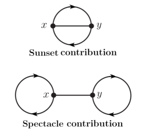
Figure 1: Graphical representation of the sunset and spectacle contributions.

With the choice $\Gamma=C\gamma_{4}$, and for gauge group SU(2), which we consider in the numerical work, the expressions are

$$B^{\pm}_{Sset}(x,y)=-\varepsilon_{abc}\varepsilon_{a^{\prime}b^{\prime}c^{\prime}} (C\gamma_{4})^{\beta\gamma}(C\gamma_{4})^{\beta^{\prime}\gamma^{\prime}}P_{\pm}^{\alpha\alpha^{\prime}}$$

$$\langle +2\Delta^{\alpha\alpha^{\prime}}_{aa^{\prime}}(x,y)\Delta^{\beta\beta^{\prime}}_{bb^{\prime}}(x,y)\Delta^{\gamma\gamma^{\prime}}_{cc^{\prime}}(x,y)$$

$$+4\Delta^{\alpha\beta^{\prime}}_{ab^{\prime}}(x,y)\Delta^{\beta\gamma^{\prime}}_{bc^{\prime}}(x,y)\Delta^{\gamma\alpha^{\prime}}_{ca^{\prime}}(x,y)\rangle,$$ (4)

and

$$B^{\pm}_{Spec}(x,y)=-\varepsilon_{abc}\varepsilon_{a^{\prime}b^{\prime}c^{\prime}} (C\gamma_{4})^{\beta\gamma}(C\gamma_{4})^{\beta^{\prime}\gamma^{\prime}}P_{\pm}^{\alpha\alpha^{\prime}}$$

$$\langle +2\Delta^{\alpha\beta}_{ab}(x,x)\Delta^{\delta\alpha^{\prime}}_{ca^{\prime}}(x,y)\Delta^{\delta^{\prime}\beta^{\prime}}_{c^{\prime}b^{\prime}}(y,y)C^{\gamma\delta}C^{\delta^{\prime}\gamma^{\prime}}$$

$$+4\Delta^{\alpha\beta}_{ab}(x,x)\Delta^{\beta^{\prime}\gamma}_{b^{\prime}c}(y,x)\Delta^{\gamma^{\prime}\alpha^{\prime}}_{c^{\prime}a^{\prime}}(y,y)$$

$$+1\Delta^{\alpha\alpha^{\prime}}_{aa^{\prime}}(x,y)\Delta^{\beta\delta}_{bc}(x,x)\Delta^{\delta^{\prime}\beta^{\prime}}_{c^{\prime}b^{\prime}}(y,y)C^{\gamma\delta}C^{\delta^{\prime}\gamma^{\prime}}$$

$$+2\Delta^{\alpha\delta^{\prime}}_{ac^{\prime}}(x,y)\Delta^{\beta\delta}_{bc}(x,x)\Delta^{\beta^{\prime}\alpha^{\prime}}_{b^{\prime}a^{\prime}}(y,y)C^{\gamma\delta}C^{\delta^{\prime}\gamma^{\prime}}\rangle.$$ (5)

Here $P_{\pm}$ denotes a parity projection; for zero momentum states it is defined as $P_{\pm}=\frac{1}{2}(1\pm\gamma_{4})$ [14]. $\varepsilon_{abc}$ are the totally antisymmetric structure constants for SU(2).

3 Numerical results

In the present section numerical results for baryon correlation functions and corresponding masses for gauge group SU(2) will be discussed. The numerically intensive and non-trivial task is to compute the inverse of the Wilson-Dirac operator. The fermion propagators appearing in the “sunset piece” are obtained from point sources using standard techniques. The all-to-all propagators appearing in the “spectacle piece” are calculated using the stochastic estimator technique. A combination of 80 stochastic estimators and 200 lowest eigenvalues has been used to minimize the stochastic noise. These parameters are optimized compared to the first test presented in Ref. [12] to improve the signal. As the spectacle contribution is still noisy, we used several sources placed randomly at all time slices of the lattice. After computing both contributions separately, they are added up for each configuration to obtain the full correlation function. We measured the baryon correlator for lattice volume $24^{3}\times 48$ at $\beta=1.75$ and $\kappa=0.14925$ on 1757 configurations. Numerical results for positive and negative parity correlation functions are shown in Fig. 2. Statistical errors have been estimated by the Jackknife method. To remove the autocorrelation along the Monte-Carlo time the data blocking method, with an optimal binlength of 50, has been used.

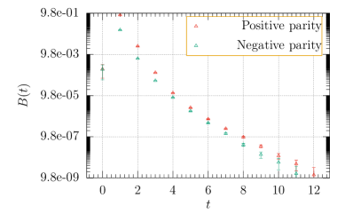
(a) Sunset contribution only.

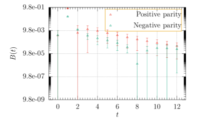
(b) Both sunset and spectacle contributions.

Figure 2: Numerical results for the positive and negative parity baryon correlation functions at $\beta=1.75$ and $\kappa=0.14925$.

In order to obtain estimates for the masses of baryonic states, the effective mass of positive and negative parity baryons is plotted as a function of time-slice distance, and is shown in Fig. 3. For precise results, a $\sinh$ function is fitted to the numerical data and a fit range $t\in\{4,9\}$ for both parities is considered. Masses obtained from the above fit ranges are shown in Tab. 1.

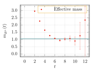
(a) Sunset: Effective mass of positive parity baryon.

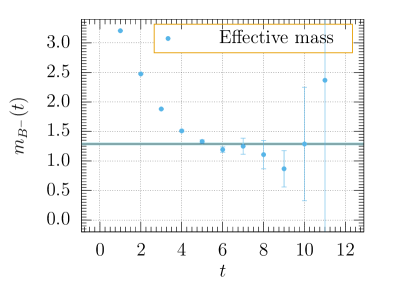
(b) Sunset: Effective mass of negative parity baryon.

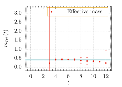
(c) Full: Effective mass of positive parity baryon.

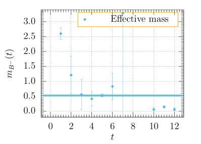
(d) Full: Effective mass of negative parity baryon.

Figure 3: Numerical results for the effective masses at $\beta=1.75$ and $\kappa=0.14925$.

Bound state	Mass (in lattice units)
$m_{B^{+}}$	0.4207(083)
$m_{B^{-}}$	0.5429(263)

Table 1: Masses of the positive and negative parity baryons in $\mathcal{N}$=1 SUSY Yang-Mills theory at $\beta=1.75$ and $\kappa=0.14925$.

4 Conclusion and outlook

We presented numerical results for positive and negative parity baryon correlators and their corresponding masses in lattice units for the gauge group SU(2). Both masses are different as expected. They are still at finite gluino mass and lattice spacing. In the next step we will measure the baryon masses from ensembles produced at different bare gluino masses, which allows to perform chiral extrapolations. In the future we plan to measure the masses for the gauge group SU(3), where we have better statistics and a well controlled continuum limit.

References

- [1] G. Curci and G. Veneziano, Nucl. Phys. B 292 (1987) 555.
-
[2]
S. Musberg, G. Münster and S. Piemonte,
JHEP 1305 (2013) 143,
[arXiv: 1304.5741[hep-lat]]. - [3] G. Veneziano and S. Yankielowicz, Phys. Lett. B 113 (1982) 231.
- [4] G. R. Farrar, G. Gabadadze and M. Schwetz, Phys. Rev. D 58 (1998) 015009, [arXiv: hep-th/9711166 ].
- [5] G. Bergner, P. Giudice, I. Montvay, G. Münster and S. Piemonte, JHEP 1603 (2016) 080, [arXiv: 1512.07014[hep-lat]].
- [6] S. Ali, G. Bergner, H. Gerber, P. Giudice, S. Kuberski, I. Montvay, G. Münster and S. Piemonte, EPJ Web Conf. 175 (2018) 08016, [arXiv: 1710.07464[hep-lat]].
- [7] S. Ali, G. Bergner, H. Gerber, P. Giudice, I. Montvay, G. Münster, S. Piemonte and P. Scior, JHEP 1803 (2018) 113, [arXiv: 1801.08062[hep-lat]].
- [8] S. Ali, G. Bergner, H. Gerber, S. Kuberski, I. Montvay, G. Münster, S. Piemonte and P. Scior, JHEP 1904 (2019) 150, [arXiv: 1901.02416[hep-lat]].
- [9] S. Ali, G. Bergner, H. Gerber, I. Montvay, G. Münster, S. Piemonte and P. Scior, Phys. Rev. Lett. 122 (2019) 2216011, [arXiv: 1902.11127[hep-lat]].
- [10] S. Ali, G. Bergner, H. Gerber, I. Montvay, G. Münster, S. Piemonte and P. Scior, Eur. Phys. J. C 78 (2018) 404, [arXiv: 1802.07067[hep-lat]].
- [11] S. Ali, G. Bergner, H. Gerber, I. Montvay, G. Münster, S. Piemonte and P. Scior, Eur. Phys. J. C 80 (2020) 548, [arXiv: 2003.04110[hep-lat]].
- [12] S. Ali, G. Bergner, H. Gerber, C. Lopez, I. Montvay, G. Münster, S. Piemonte and P. Scior, PoS(LATTICE 2018) 207, [arXiv: 1811.02297[hep-lat]].
- [13] S. Ali, PhD thesis, University of Münster, June, 2019.
- [14] I. Montvay and G. Münster, Quantum Fields on a Lattice, Cambridge University Press, 1994.