Abstract  In this paper we solve the longstanding Gaussian curvature conjecture of a minimal graph $S$ over the unit disk. This conjecture states the following. For any minimal graph lying above the entire unit disk, the Gaussian curvature at the point above the origin satisfies the sharp inequality $|\mathcal{K}|<\pi^{2}/2$. The conjecture is first reduced to the estimation of the Gaussian curvature of certain Scherk type minimal surfaces over some bicentric quadrilaterals inscribed in the unit disk containing the origin. Then we make a sharp estimate of the Gaussian curvature of those minimal surfaces over those bicentric quadrilaterals at the point above the zero. Our proof uses complex-analytic methods since minimal surfaces that we consider allow conformal harmonic parameterization.

Keywords  Conformal minimal surface, minimal graph, curvature

MSC (2010):  53A10, 32B15, 32E30, 32H02

Date:

1.  Introduction and the main result

Let $D(w_{0},R)$ be a dist in $\mathbf{R}^{2}$ and let $\mathbf{f}:D(w_{0},R)\to\mathbf{R}$ be a $\mathbf{C}^{2}$ function that solves the minimal surface equation

$$\mathbf{f}_{uu}(1+\mathbf{f}_{v}^{2})-2\mathbf{f}_{u}\mathbf{f}_{v}\mathbf{f}_{uv}+\mathbf{f}_{vv}(1+\mathbf{f}_{u}^{2})=0.$$

The graph of $\mathbf{f}$: $S=\mathrm{Graph}_{\mathbf{f}}=\{(u,v,\mathbf{f}(u,v))\}$ is called a minimal graph in $\mathbf{R}^{3}$ over the disk $D(w_{0},R).$ Then the Gaussian curvature of the graph $S$ at a point $P=(u,v,\mathbf{f}(u,v))$ is given by

$$\mathcal{K}(P)=\frac{\mathbf{f}_{uu}\mathbf{f}_{vv}-\mathbf{f}_{uv}^{2}}{(1+\mathbf{f}^{2}_{u}+\mathbf{f}_{v}^{2})^{2}}.$$

Assume that $\xi$ is a point above $w_{0}$. A longstanding open problem in the theory of minimal surfaces is to determine the precise value of the constant $c_{0}$ in the inequality

(1.1) $$|\mathcal{K}(\xi)|\leq\frac{c_{0}}{R^{2}}.$$

This problem has its origin in 1952 [9]. More precisely, E. Heinz in [9] proved the famous Bernstein theorem (see also the monograph by T. Colding and W. Minicozzi II [3, Theorem 2.3]) by proving that there is a positive constant $c_{0}$ so that (1.1) holds. A number of improvements and generalizations have been obtained by several authors: E. Hopf [11], R. Finn and R. Osserman [6], J. C. C. Nitsche [16], R. Hall [7, 8]. E. Hopf [11] (1953) asked for optimality of the constant $c_{0}$ in the so-called Heinz inequality (1.1) and he proposed the following conjecture

Conjecture 1.1.

(1.2) $$c_{0}=\frac{\pi^{2}}{2}.$$

This conjecture has been proved by Finn and Osserman [6] under the additional assumption that the tangential plane of the minimal surface is horizontal at the point $\xi$. Further J. C. C. Nitsche [16] proved (1.2) for symmetric minimal surfaces.

This conjecture has also been mentioned by Duren in [4, p. 185], Finch in [5, p. 401] and Kovalev and Yang in [14].

In this paper we solve the Conjecture 1.2 by proving the following theorem:

Theorem 1.2.

Assume that $S$ is a minimal graph over the disk $D(w_{0},R)$, where $\xi$ is a point above $w_{0}$. Then the sharp inequality

(1.3) $$|\mathcal{K}(\xi)|<\frac{\pi^{2}}{2}\frac{1}{R^{2}}$$

holds. The equality in (1.3) cannot be attained.

It must be emphasizes that, the proof os this conjecture proves a beautiful connection between two classical mathematical topics differential geometry and complex analysis in proving a property for minimal surfaces that represents the most beautiful geometrical objects. The first step toward the proof of the conjecture is the following result (Theorem 1.4) which has been announced by the first author in the unpublished manuscript [13] in order to get some partial results concerning the conjecture. Since the other results from that preprint are obsolete, and for the sake of completeness argument the first author decided to withdraw that manuscript and to insert its main result in this paper. In order to formulate Theorem 1.4 we use the following:

Definition 1.3.

Assume that $Q=Q(a,b,c,d)$ is a bicentric quadrilateral inscribed in the unit disk $\mathbb{D}$. A minimal graph $S=\{(u,v,\mathbf{f}(u,v)),(u,v)\in Q\}$ over the quadrilateral $Q$ is called a Scherk type surface if it satisfies $\mathbf{f}(u,v)\rightarrow+\infty$ when $(u,v)\rightarrow\zeta\in(a,b)\cup(c,d)$ and $\mathbf{f}(u,v)\rightarrow-\infty$ when $(u,v)\rightarrow\zeta\in(b,c)\cup(a,d)$ .

Theorem 1.4.

For every $w\in\mathbb{D}$, there exist four different points $a_{0},a_{1},a_{2},a_{3}\in\mathbf{T}$ and a harmonic mapping $f$ of the unit disk onto the quadrilateral $Q(a_{0},a_{1},a_{2},a_{3})$ that solves the Beltrami equation

(1.4) $$\bar{f}_{z}(z)=\left(\frac{w+\frac{\mathfrak{i}\left(1-w^{4}\right)z}{\left|1-w^{4}\right|}}{1+\frac{\mathfrak{i}\overline{w}\left(1-w^{4}\right)z}{\left|1-w^{4}\right|}}\right)^{2}f_{z}(z),$$

$|z|<1$ and satisfies the initial condition $f(0)=0$, $f_{z}(0)>0$. The mapping $f$ gives rise to a Scherk type minimal surface $S^{\diamond}:\zeta=\mathbf{f}^{\diamond}(u,v)$ over the quadrilateral $Q(a_{0},a_{1},a_{2},a_{3})$, containing the point $\xi=(0,0,0)$ above the origin so that its Gaussian normal is

$$\mathbf{n}^{\diamond}_{\xi}=-\frac{1}{1+|w|^{2}}(2\Im w,2\Re w,-1+|w|^{2}),$$

and such that $D_{uv}\mathbf{f}^{\diamond}(0,0)=0$. Moreover, every other non-parametric minimal surface $S:$ $\zeta=\mathbf{f}(u,v)$ over the unit disk, containing the point $\xi$ above zero, with $\mathbf{n}_{\xi}=\mathbf{n}^{\diamond}_{\xi}$ and $D_{uv}\mathbf{f}(0,0)=0$ satisfies the sharp inequality

$$|\mathcal{K}_{S}(\xi)|<|\mathcal{K}_{S^{\diamond}}(\xi)|.$$

In order to prove Theorem 1.2, we will construct all Scherk type surfaces over the unit disk and estimate their curvature at the point above zero. Namely we will prove the following theorem:

Theorem 1.5.

Assume that $Q(b_{0},b_{1},b_{2},b_{3})$ is a quadrilateral inscribed in the unit disk and assume that $0\in Q(b_{0},b_{1},b_{2},b_{3})$. Assume also that $\zeta(u,v)=(u,v,\mathbf{f}^{\ast}(u,v))$ is a minimal surface above $Q(b_{0},b_{1},b_{2},b_{3})$ with $\xi$ above $0$. Then

$$|\mathcal{K}(\xi)|\leq\frac{\pi^{2}}{2}.$$

1.1.  Organization of the paper

This section contains one more subsection where we express the Gaussian curvature in terms of Enneper–Weierstrass. In the sequel we have three more sections. Proofs of Theorem 1.5 and Theorem 1.4 are the main content of this paper. They are involved and contains a number of subtle relations. The proof of Theorem 1.4 is given in Section 2. The proof of Theorem 1.5 is presented in Section 4. We prepare for the proof in Section 3 by describing all Scherk type surfaces over the unit disk. Having Theorem 1.4 and Theorem 1.5, the proof of Theorem 1.2 is a simple matter.

Proof of Theorem 1.2.

Assume that $S=\{(u,v,\mathbf{f}(u,v))\}$ is an arbitrary minimal surface above the unit disk, and assume that $\xi$ is the point above $w_{0}$. Assume, without loss of generality, that $R=1$ and $w_{0}=0$. Let $v=e^{\mathfrak{i}\tau}$ and $\mathbf{f}^{\tau}(w)=\mathbf{f}(e^{\mathfrak{i}\tau}w)$, then

$$\mathbf{f}^{\tau}_{u}(0,0)=\cos\tau\,\mathbf{f}_{u}(0,0)+\sin\tau\,\mathbf{f}_{v}(0,0).$$

Further

$$\mathbf{f}^{\tau}_{uv}(0,0)=\cos(2\tau)\mathbf{f}_{uv}(0,0)+\cos(\tau)\sin(\tau)\left(-\mathbf{f}_{vv}(0,0)+\mathbf{f}_{uu}(0,0)\right).$$

Since $\mathbf{f}^{\pi/2}_{uv}(0,0)=-\mathbf{f}_{uv}(0,0)$, there is $\tau$ so that $\mathbf{f}^{\tau}_{uv}(0,0)=0$. In other words the new minimal surface $S^{\tau}:\zeta(u,v)=(u,v,\mathbf{f}^{\tau}(u,v))$ satisfies the condition $\mathbf{f}^{\tau}_{uv}(0,0)=0$ of Theorem 1.4. Let $\mathbf{n}$ be its unit normal at $\xi=(0,0,\mathbf{f}^{\tau}(0,0))=(0,0,0)$. Then, from Theorem 1.4 there is a Scherk type surface $S^{\diamond}:\zeta(u,v)=(u,v,\mathbf{f}^{\diamond}(u,v))$, above a quadrilateral $Q(a_{0},a_{1},a_{2},a_{3})$ having the unit normal equal to $\mathbf{n}$ at $(0,0,0)$. Moreover

$$|\mathcal{K}_{S^{\tau}}(\mathbf{w})|<|\mathcal{K}_{S^{\diamond}}(\mathbf{w})|.$$

On the other hand by Theorem 1.5 $|\mathcal{K}_{S^{\diamond}}(\mathbf{w})|\leq\pi^{2}/2$ and this finishes the proof. ∎

1.2.  Minimal surfaces and Gaussian curvature

Let $M\subset\mathbb{R}^{3}=\mathbb{C}\times\mathbb{R}$ be a minimal graph lying over the unit disc $\mathbb{D}\subset\mathbb{C}$. Let $w=(w_{1},w_{2},w_{3}):\mathbb{D}\to M$ be a conformal harmonic parameterization of $M$ with $w(0)=0$. Its projection $(w_{1},w_{2}):\mathbb{D}\to\mathbb{D}$ is a harmonic diffeomorphism of the disc which may be assumed to preserve orientation. Let $z$ be a complex variable in $\mathbb{D}$, and write $w_{1}+\mathfrak{i}w_{2}=f$ in the complex notation. We denote by $f_{z}=\partial f/\partial z$ and $f_{\bar{z}}=\partial f/\partial\bar{z}$ the Wirtinger derivatives of $f$. The function $\omega$ defined by

(1.5) $$\overline{f_{\bar{z}}}=\omega f_{z}$$

is called the second Beltrami coefficient of $f$, and the above equation is the second Beltrami equation with $f$ as a solution. Observe that $\bar{f}_{z}=\overline{f_{\bar{z}}}$ and this notation will be used in the sequel.

Orientability of $f$ is equivalent to $\mathrm{Jac}(f)=|f_{z}|^{2}-|f_{\bar{z}}|^{2}>0$, hence to $|\omega|<1$ on $\mathbb{D}$. Furthermore, the function $\omega$ is holomorphic whenever $f$ is harmonic and orientation preserving. (In general, it is meromorphic when $f$ is harmonic.) To see this, let

(1.6) $$u+\mathfrak{i}v=f=h+\overline{g}$$

be the canonical decomposition of the harmonic map $f:\mathbb{D}\to\mathbb{D}$, where $h$ and $g$ are holomorphic functions on the disk. Then,

(1.7) $$f_{z}=h^{\prime},\quad\ f_{\bar{z}}=\overline{g}_{\bar{z}}=\overline{g^{\prime}},\quad\ \omega=\overline{f_{\bar{z}}}/f_{z}=g^{\prime}/h^{\prime}.$$

In particular, the second Beltrami coefficient $\omega$ equals the meromorphic function $g^{\prime}/h^{\prime}$ on $\mathbb{D}$. In our case we have $|\omega|<1$, so it is a holomorphic map $\omega:\mathbb{D}\to\mathbb{D}$.

We now consider the Enneper–Weierstrass representation of the minimal graph $\varpi=(u,v,T):\mathbb{D}\to M\subset\mathbb{D}\times\mathbb{R}$ over $f$, following Duren [4, p. 183]. We have

$$u(z) = \Re f(z)=\Re\int_{0}^{z}\phi_{1}(\zeta)d\zeta$$

$$v(z) = \Im f(z)=\Re\int_{0}^{z}\phi_{2}(\zeta)d\zeta$$

$$T(z) = \Re\int_{0}^{z}\phi_{3}(\zeta)d\zeta$$

where

$$\phi_{1} = 2(u)_{z}=2(\Re f)_{z}=(h+\bar{g}+\bar{h}+g)_{z}=h^{\prime}+g^{\prime},$$

$$\phi_{2} = 2(v)_{z}=2(\Im f)_{z}=\mathfrak{i}(\bar{h}+g-h-\bar{g})_{z}=\mathfrak{i}(g^{\prime}-h^{\prime}),$$

$$\phi_{3} = 2(T)_{z}=\sqrt{-\phi_{1}^{2}-\phi_{2}^{2}}=\pm 2\mathfrak{i}\sqrt{h^{\prime}g^{\prime}}.$$

The last equation follows from the identity $\phi_{1}^{2}+\phi_{2}^{2}+\phi_{3}^{2}=0$ which is satisfied by the Enneper–Weierstrass datum $\phi=(\phi_{1},\phi_{2},\phi_{3})=2\partial w$ of any conformal minimal (equivalently, conformal harmonic) immersion $w:D\to\mathbb{R}^{3}$ from a conformal surface $D$. Let us introduce the notation $\mathbf{p}=f_{z}$. We have

(1.8) $$\mathbf{p}=f_{z}=(\Re f)_{z}+\mathfrak{i}(\Im f)_{z}=\frac{1}{2}(h^{\prime}+g^{\prime}+h^{\prime}-g^{\prime})=h^{\prime}.$$

By using $\omega=\overline{f_{\bar{z}}}/f_{z}=g^{\prime}/h^{\prime}$ (see (1.7)), it follows that

$$\phi_{1}=h^{\prime}+g^{\prime}=\mathbf{p}(1+\omega),\quad\phi_{2}=-\mathfrak{i}(h^{\prime}-g^{\prime})=-\mathfrak{i}\mathbf{p}(1-\omega),\quad\phi_{3}=\pm 2\mathfrak{i}\mathbf{p}\sqrt{\omega}.$$

From the formula for $\phi_{3}$ we infer that $\omega$ has a well-defined holomorphic square root:

(1.9) $$\omega=\mathbf{q}^{2},\qquad\mathbf{q}:\mathbb{D}\to\mathbb{D}\ \ \text{holomorphic}.$$

In terms of the Enneper–Weierstrass parameters $(\mathbf{p},\mathbf{q})$ given by (1.8) and (1.9) we obtain

(1.10) $$\phi_{1}=\mathbf{p}(1+\mathbf{q}^{2}),\quad\phi_{2}=-\mathfrak{i}\mathbf{p}(1-\mathbf{q}^{2}),\quad\phi_{3}=-2\mathfrak{i}\mathbf{p}\mathbf{q}.$$

(The choice of sign in $\phi_{3}$ is a matter of convenience; since we have two choices of sign for $\mathbf{q}$ in (1.9), this does not cause any loss of generality.) Hence,

$$\varpi(z)=\left(\Re f(z),\Im f(z),\Im\int_{0}^{z}2\mathbf{p}(\zeta)\mathbf{q}(\zeta)d\zeta\right),\quad z\in\mathbb{D}.$$

The curvature $\mathcal{K}$ of the minimal graph $M$ is expressed in terms of $(h,g,\omega)$ (1.7), and in terms of the Enneper–Weierstrass parameters $(\mathbf{p},\mathbf{q})$, by

(1.11) $$\mathcal{K}=-\frac{|\omega^{\prime}|^{2}}{|h^{\prime}g^{\prime}|(1+|\omega|)^{4}}=-\frac{4|\mathbf{q}^{\prime}|^{2}}{|\mathbf{p}|^{2}(1+|\mathbf{q}|^{2})^{4}},$$

where $\mathbf{p}=f_{z}$ and $\omega=\mathbf{q}^{2}=\overline{f_{\bar{z}}}/f_{z}$. (See Duren [4, p. 184].) For a slightly different formula concerning the expression of Gaussian curvature we refer to the monographs by Alarcon, Forstnerič and Lopez [1, Sec. 2.6].

2.  Proof of Theorem 1.4

Proof of Theorem 1.4.

In order to prove Theorem 1.4, we will derive a useful formula for $\mathbf{f}_{uv}$, of a non-parametric minimal surface $w=\mathbf{f}(u,v)$. Namely we will express $\mathbf{f}_{uv}$ as a function of Enneper-Weisstrass parameters. Assume that $q(z)=a(z)+\mathfrak{i}b(z)=\sqrt{\omega(z)}$ and $p$ are Enneper-Weisstrass parameters of a minimal disk $S=\{(u(z),v(z),T(z)),z\in\mathbb{D}\}=\{(u,v,\mathbf{f}(u,v)):(u,v)\in\mathbb{D}\}$ over the unit disk. Here $f=u+iv$ and $\bar{f}_{z}=\omega(z)f_{z}$.

Then the unit normal at $\mathbf{w}\in S$, in view of [4, p. 169] is given by

$$\mathbf{n}_{\mathbf{w}}=-\frac{1}{1+|q(z)|^{2}}(2\Im q(z),2\Re q(z),-1+|q(z)|^{2}).$$

It is also given by the formula

$$\mathbf{n}_{\mathbf{w}}=\frac{1}{\sqrt{1+\mathbf{f}_{u}^{2}+\mathbf{f}_{v}^{2}}}\left(-\mathbf{f}_{u},-\mathbf{f}_{v},1\right).$$

Then we have the relations

(2.1) $$\mathbf{f}_{v}(u(x,y),v(x,y))=\frac{2a(x,y)}{-1+a(x,y)^{2}+b(x,y)^{2}}$$

(2.2) $$\mathbf{f}_{u}(u(x,y),v(x,y))=\frac{2b(x,y)}{-1+a(x,y)^{2}+b(x,y)^{2}}.$$

By differentiating (2.1) and (2.2) w.r.t. $x$ we obtain the equations

(2.3) $$v_{x}\mathbf{f}_{uv}(u,v)+u_{x}\mathbf{f}_{uu}(u,v)=-\frac{4aba_{x}+2\left(1-a^{2}+b^{2}\right)b_{x}}{\left(-1+a^{2}+b^{2}\right)^{2}}$$

(2.4) $$v_{x}\mathbf{f}_{vv}(u,v)+u_{x}\mathbf{f}_{uv}(u,v)=-\frac{4abb_{x}+2\left(1-a^{2}+b^{2}\right)a_{x}}{\left(-1+a^{2}+b^{2}\right)^{2}}.$$

Now recall the minimal surface equation

(2.5) $$\left(1+\mathbf{f}^{2}_{u}(u,v)^{2}\right)\mathbf{f}_{vv}(u,v)+\left(1+\mathbf{f}^{2}_{v}(u,v)^{2}\right)\mathbf{f}_{uu}(u,v)=2\mathbf{f}_{v}(u,v)\mathbf{f}_{u}(u,v)\mathbf{f}_{uv}(u,v)$$

From (2.1), (2.2), (2.3),(2.4) and (2.5) we get

$$\mathbf{f}_{uv}=\frac{M}{N}$$

where

$$\begin{split}M&=-2(a^{4}+2a^{2}(-1+b^{2})+(1+b^{2})^{2})((1+a^{2}-b^{2})a_{x}+2abb_{x})u_{x}\\ &-2((1+a^{2})^{2}+2(-1+a^{2})b^{2}+b^{4})(2aba_{x}+(1-a^{2}+b^{2})b_{x})v_{x}\end{split}$$

and

$$\begin{split}N&=(1-a^{2}-b^{2})^{2}\\ &\times((a^{4}-2a^{2}(1-b^{2})+(1+b^{2})^{2})u_{x}^{2}+8abu_{x}v_{x}+((1+a^{2})^{2}-2(1-a^{2})b^{2}+b^{4})v_{x}^{2}).\end{split}$$

Let $q(z)=a+\mathfrak{i}b=re^{it}$, $q^{\prime}(z)=a_{x}+\mathfrak{i}b_{x}=Re^{is}$ and $p=Pe^{im}$. Because $u_{x}=\Re(p(1+q^{2}))$, and $v_{x}=-\Re(\mathfrak{i}p(1-q^{2}))$, after straightforward calculation we get

$$\mathbf{f}_{uv}=-\frac{2R\left(\cos[m-s]-r^{4}\cos[m-s+4t]\right)}{P\left(1-r^{2}\right)^{3}\left(1+r^{2}\right)}$$

which can be written as

(2.6) $$\mathbf{f}_{uv}=-\frac{2\Re\left[p(1-q^{4})\overline{q^{\prime}}\right]}{|p|^{2}(1-|q|^{2})^{3}(1+|q|^{2})}.$$

Now we continue to prove Theorem 1.4. The solution of (1.4) with such initial conditions exists and is unique [2, Theorem A& Theorem 1] and maps the unit disk onto a quadrilateral $Q(a_{0},a_{1},a_{2},a_{3})$ whose vertices $a_{0},a_{1},a_{2},a_{3}$, $a_{4}=a_{0}$ belongs to the unit circle. Moreover by [2, Theorem B], there are four points $b_{k}=e^{\mathfrak{i}\alpha_{k}},\ k=0,1,2,3$, $b_{4}=b_{0},b_{5}=b_{1}$,

$$F(e^{it})=\sum_{k=1}^{4}a_{k}I_{(\alpha_{k},\alpha_{k+1})}(t).$$

Here $F$ is the boundary function of $f$. Therefore ([Duren, p. 63]) we can conclude that

$$f_{z}(z)=\sum_{k=1}^{4}\frac{d_{k}}{z-b_{k}},$$

and that

$$\bar{f}_{z}(z)=-\sum_{k=1}^{4}\frac{\overline{d_{k}}}{z-b_{k}},$$

where

$$d_{k}=\frac{a_{k}-a_{k+1}}{2\pi\mathfrak{i}}.$$

Therefore the third coordinate of conformal parameterisation is

$$T(z)=\pm 2\Re\mathfrak{i}\int_{0}^{z}\sqrt{f_{z}\bar{f}_{z}}dz$$

thus when $z$ is close to $b_{k}$, then

$$T(z)=\pm|d_{k}|^{2}\log|1-z/b_{k}|+O(z-b_{k}).$$

Thus when $z\to b_{k}$, $T(z)\to\pm\infty$. This implies that $\mathbf{f}(z)\to\pm\infty$ if $z\to a\in(a_{k},a_{k+1})$. Since

$$q(z)=\frac{w+\frac{\mathfrak{i}\left(1-w^{4}\right)z}{\left|1-w^{4}\right|}}{1+\frac{\mathfrak{i}\overline{w}\left(1-w^{4}\right)z}{\left|1-w^{4}\right|}},$$

we get

$$q(0)=w\ \ \text{and}\ \ q^{\prime}(0)=\frac{\mathfrak{i}\left(1-w^{4}\right)\left(1-|w|^{2}\right)}{\left|1-w^{4}\right|}.$$

Further

$$p(0)(1-q(0)^{4})\overline{q^{\prime}(0)}=-\mathfrak{i}f_{z}(0)|1-w^{4}|(1-|w|^{2}).$$

So in view of the formula (2.6) we conclude $\mathbf{f}^{\diamond}_{uv}=0.$

Now we assert that

(2.7) $$|\mathcal{K}_{S}(\mathbf{w})|<|\mathcal{K}_{S^{\diamond}}(\mathbf{w})|.$$

Assume the converse $|\mathcal{K}_{S}(\mathbf{w})|\geq|\mathcal{K}_{S^{\diamond}}(\mathbf{w})|$ and argue by a contradiction. Then as in [6], by using the dilatation $L(\zeta)=\lambda\zeta$ for some $\lambda\geq 1$ we get the surface

$$S_{1}=L(S)=\{(u,v,\lambda\mathbf{f}\left(\frac{u}{\lambda},\frac{v}{\lambda}\right):|u+\mathfrak{i}v|<{\lambda}\},$$

whose Gaussian curvature

$$\mathcal{K}_{1}(\mathbf{w})=\frac{\frac{1}{\lambda^{2}}\left(\mathbf{f}_{uu}(0,0)\mathbf{f}_{vv}(0,0)-\mathbf{f}_{uv}(0,0)^{2}\right)}{(1+\mathbf{f}_{u}(0,0)^{2}+\mathbf{f}_{v}(0,0)^{2})^{2}}.$$

Observe that such transformation does not change the unit normal at $\mathbf{w}$.

Then there is $\lambda_{\ast}\geq 1$ so that $\mathcal{K}_{1}(\mathbf{w})=\mathcal{K}_{S^{\diamond}}(\mathbf{w})$. Let

$$\mathbf{f}^{\ast}(u,v)=\lambda_{\ast}\mathbf{f}\left(\frac{u}{\lambda_{\ast}},\frac{v}{\lambda_{\ast}}\right).$$

From $\mathbf{n}_{\diamond}=\mathbf{n}_{\ast}$ we get

(2.8) $$\mathbf{f}^{\diamond}_{u}(0,0)=\mathbf{f}^{\ast}_{u}(0,0),\ \mathbf{f}^{\diamond}_{v}(0,0)=\mathbf{f}^{\ast}_{v}(0,0).\$$

Further we have

$$(1+(\mathbf{f}^{\ast}_{u}(0,0))^{2})\mathbf{f}^{\ast}_{vv}(0,0)-2\mathbf{f}^{\ast}_{u}(0,0)\mathbf{f}^{\ast}_{v}(0,0)\mathbf{f}^{\ast}_{uv}(0,0)+(1+(\mathbf{f}^{\ast}_{v}(0,0))^{2})\mathbf{f}^{\ast}_{uu}(0,0)=0,$$

$$(1+(\mathbf{f}^{\diamond}_{u}(0,0))^{2})\mathbf{f}^{\diamond}_{vv}(0,0)-2\mathbf{f}^{\diamond}_{u}(0,0)\mathbf{f}^{\diamond}_{v}(0,0)\mathbf{f}^{\diamond}_{uv}(0,0)+(1+(\mathbf{f}^{\diamond}_{v}(0,0))^{2})\mathbf{f}^{\diamond}_{uu}(0,0)=0,$$

$$\mathbf{f}^{\diamond}_{uv}(0,0)=\mathbf{f}^{\ast}_{uv}(0,0)$$

and the equation

$$\frac{\left(\mathbf{f}^{\ast}_{uu}(0,0)\mathbf{f}^{\ast}_{vv}(0,0)-\mathbf{f}^{\ast}_{uv}(0,0)^{2}\right)}{(1+\mathbf{f}^{\ast}_{u}(0,0)^{2}+\mathbf{f}^{\ast}_{v}(0,0)^{2})^{2}}=\frac{\left(\mathbf{f}^{\diamond}_{uu}(0,0)\mathbf{f}^{\diamond}_{vv}(0,0)-\mathbf{f}^{\diamond}_{uv}(0,0)^{2}\right)}{(1+\mathbf{f}^{\diamond}_{u}(0,0)^{2}+\mathbf{f}^{\diamond}_{v}(0,0)^{2})^{2}}.$$

We can also w.l.g. assume that $\mathbf{f}^{\ast}_{uu}$ and $\mathbf{f}^{\diamond}_{uu}$ as well as $\mathbf{f}^{\ast}_{vv}$ and $\mathbf{f}^{\diamond}_{vv}$ have the same sign. If not, then we choose $\lambda_{\ast}\leq-1$ and repeat the previous procedure with

$$S_{1}=L(S)=\{(u,v,\lambda\mathbf{f}\left(\frac{u}{\lambda},\frac{v}{\lambda}\right):|u+\mathfrak{i}v|<{|\lambda|}\}.$$

Thus the function $F(u,v)=\mathbf{f}^{\ast}(u,v)-\mathbf{f}^{\diamond}(u,v)$ has all derivatives up to the order $2$ equal to zero in the point $w=0$.

To continue the proof we use the following lemma

Lemma 2.1.

Assume that the quadrilateral $Q=Q(a,b,c,d)$ is inscribed in the unit disk, and assume that $\zeta=\mathbf{f}(u,v)$ is a Scherk’s type minimal surface $S$ above $Q$. i.e. assume that $\mathbf{f}(u,v)\to+\infty$ when $\zeta=u+iv\to w\in(a,b)\cup(c,d)$ and $\mathbf{f}(u,v)\to-\infty$ when $\zeta=u+iv\to w\in(b,c)\cup(a,d)$. Then there is not any other bounded minimal graph $\zeta=\mathbf{f}_{1}(u,v)$ over a domain $\Omega$ that contains $Q$ which has the same Gaussian curvature, the same Gaussian normal, and the same mixed derivative at the same point $\mathbf{w}\in Q$ as the given surface $S$.

Proof of Lemma 2.1.

We observe that [6, Proof of Proposition 1] works for every Scherk’s type minimal surface, so if we would have a bounded minimal surface having the all derivatives ap to the order 2 equal to zero, then such non-parametric parameterizations $\mathbf{f}$ and $\mathbf{f}_{1}$, in view of [6, Lemma 1] will satisfy the relation $F(z)=\mathbf{f}(z)-\mathbf{f}_{1}(z)=O(\zeta^{N}(z))$, $N\geq 3$, where $\zeta$ is a certain homeomorphism between two open sets containing $0$. Then by following the proof of [6, Proof of Proposition 1] (second part) we get that this is not possible, because Sherk’s type surface has four ”sides” but the number $2N$ is bigger or equal to $6$ which is not possible. ∎

This leads to the contradiction so (2.7) is true. ∎

3.  Two parameter family of Scherk type minimal surfaces

In this section we will describe all Scherk type surfaces over the unit disk. By the result of Jenkins and Serrin from [12] or Sheil-Small from [17] we know that the image of the corresponding harmonic function $f$ is bicentric quadrilateral. Also, after the construction we will find the explicit values of the certain quantities needed for the calculation of the Gaussian curvature.

Harmonic mappings with given dilatation, especially when Beltrami coefficient is a Blaschke product (as it is our case), are investigated in many papers. Several results on the existence and the uniqueness of these and more general mappings can be found, for example, in [2], [10] [12], [17].

3.1.  Construction of the two-parameter family

We start from the following Beltrami equation:

(3.1) $$\overline{f}_{z}=z^{2}f_{z},$$

since its solution can be easily understood and described. Indeed, if $f_{1}$ is harmonic mapping and it satisfies the equation (3.1), by [2] and [17], it is a mapping of the unit disk onto a quadrilateral inscribed in the unit disk, which is a Poisson extension of a step function, determined by a set of four points on the unit circle, that defines a quadrilateral in the domain. In [17] it is proved that the sums of lengths of two non-adjacent sides of quadrilateral in co-domain are equal. Moreover, in Example 4 from the same paper the relation between the vertices of quadrilaterals in domain and co-domain is given. Precisely, if $b_{0}=1,b_{1}=e^{\mathfrak{i}s_{1}},b_{2}=e^{\mathfrak{i}s_{2}},b_{3}=e^{\mathfrak{i}s_{3}}$ and $f_{1}$ is defined as the harmonic extension of the function

$$F_{1}(\psi)=\left\{\begin{array}[]{ll}a_{1}=e^{\mathfrak{i}t_{1}},&\hbox{if $\psi\in[0,s_{1})$;}\\ a_{2}=e^{\mathfrak{i}t_{2}},&\hbox{if $\psi\in[s_{1},s_{2})$;}\\ a_{3}=e^{\mathfrak{i}t_{3}},&\hbox{if $\psi\in[s_{2},s_{3})$;}\\ a_{4}=e^{\mathfrak{i}t_{4}},&\hbox{if $\psi\in[s_{3},2\pi)$.}\end{array}\right.$$

then we have:

$$b_{k}=\epsilon_{k}\frac{|a_{k+1}-a_{k}|}{a_{k+1}-a_{k}}$$

for $k=1,2,3,4,$ $\epsilon_{1}=\epsilon_{3}=1,\epsilon_{2}=\epsilon_{4}=-1,$ $t_{5}=t_{1}+2\pi.$ From

$$a_{k+1}-a_{k}=e^{\mathfrak{i}t_{k+1}}-e^{\mathfrak{i}t_{k}}=2\mathfrak{i}\sin\frac{t_{k+1}-t_{k}}{2}e^{\mathfrak{i}\frac{t_{k+1}+t_{k}}{2}},$$

we conclude $b_{0}b_{2}+b_{1}b_{3}=0$ and

(3.2) $$b_{k}=e^{\mathfrak{i}\big{(}\frac{3\pi}{2}-\frac{t_{k+1}+t_{k}}{2}\big{)}}.$$

Hence, if we take $s_{1}=p,$ $s_{2}=q,$ then $s_{3}=\pi+q-p$,

(3.3) $$0\leq p\leq q\leq q-p+\pi\leq 2\pi.$$

Also, from the equation (3.2) we can express $t_{k}^{\prime}$s in terms of $p,q,\beta$ as $t_{1}=\frac{q+\pi}{2}+\beta-p,$ $t_{2}=\frac{5\pi-q}{2}-p-\beta,$ $t_{3}=\frac{5\pi-3q}{2}+\beta+p$ and $t_{4}=\frac{5\pi-q}{2}+p-\beta$. This follows easily.

After the rotation $R$ of the quadrilateral in co-domain for the angle $\beta+\frac{q-\pi}{2},$ we get the quadrilateral with vertices $e^{\mathfrak{i}x},e^{\mathfrak{i}y},e^{\mathfrak{i}s},e^{\mathfrak{i}p}$ where $x=q-p+2\beta,y=2\pi-p,s=2\pi-q+p+2\beta,$ and $\beta$ is a certain parameter. We will show that $\beta$ also depends on $p$ and $q.$ However, since the quadrilateral with vertices $a_{0},a_{1},a_{2},a_{3}$ is bicentric, the same holds for the new quadrilateral obtained after rotation.

Therefore, we start from the identity:

$$|e^{\mathfrak{i}p}-e^{\mathfrak{i}x}|+|e^{\mathfrak{i}y}-e^{\mathfrak{i}s}|=|e^{\mathfrak{i}x}-e^{\mathfrak{i}y}|+|e^{\mathfrak{i}s}-e^{\mathfrak{i}p}|,$$

or, equivalently:

$$\bigg{|}\sin\frac{p-x}{2}\bigg{|}+\bigg{|}\sin\frac{y-s}{2}\bigg{|}=\bigg{|}\sin\frac{x-y}{2}\bigg{|}+\bigg{|}\sin\frac{s-p}{2}\bigg{|}.$$

Inserting $x=q-p+2\beta,y=2\pi-p,s=2\pi-q+p+2\beta,$ we get

$$|\sin(\beta+\frac{q}{2}-p)|+|\sin(\beta+p-\frac{q}{2})|=|\sin(\frac{q}{2}+\beta-\pi)|+|\sin(\pi-\frac{q}{2}+\beta)|.$$

To transform this equality in more conventional form, we recall the ordering between vertices. In fact, there holds the following chain of inequalities:

(3.4) $$p\leq q-p+2\beta\leq 2\pi-p\leq 2\pi-q+p+2\beta\leq 2\pi+p,$$

which implies

$$\beta+p\geq\frac{q}{2},\beta+\frac{q}{2}\geq p,$$

$$\frac{q}{2}+\beta\leq\pi$$

and

$$\frac{q}{2}\geq\beta.$$

It further implies $\beta\geq 0$ and

$$\beta+\frac{q}{2}-p\in[0,\pi],$$

$$\beta+\frac{q}{2}\in[0,\pi]$$

and

$$0\leq\beta+p-\frac{q}{2}=\beta+\frac{q}{2}+p-q\leq\beta+\frac{q}{2}\leq\pi.$$

Hence

$$|\sin(\beta+\frac{q}{2}-p)|=\sin(\beta+\frac{q}{2}-p),\ |\sin(\frac{q}{2}+\beta-\pi)|=\sin(\frac{q}{2}+\beta),$$

and

$$|\sin(\beta+p-\frac{q}{2})|=\sin(\beta+p-\frac{q}{2}),\ \ |\sin(\pi-\frac{q}{2}+\beta)|=\sin(\pi-\frac{q}{2}+\beta).$$

Therefore,

$$\sin(\beta+\frac{q}{2}-p)+\sin(\beta+p-\frac{q}{2})=\sin(\beta+\frac{q}{2})+\sin(\frac{q}{2}-\beta)$$

and now, we easily conclude

$$\sin\beta\cos(\frac{q}{2}-p)=\cos\beta\sin\frac{q}{2},$$

i.e.

(3.5) $$\tan\beta=\frac{\sin\frac{q}{2}}{\cos(\frac{q}{2}-p)}.$$

Note that $\tilde{f}:=R(f_{1}(z))$ has the dilatation

(3.6) $$\tilde{\omega}(z)=\frac{\tilde{g}^{\prime}}{\tilde{h}^{\prime}}=-e^{-\mathfrak{i}(2\beta+q)}z^{2}.$$

We are now searching for Möbius transformation $M$ which maps

$$(z_{1},z_{2},z_{2},z_{2})=(1,e^{\mathfrak{i}\alpha},-1,-e^{\mathfrak{i}\alpha})$$

to

$$(w_{1},w_{2},w_{3},w_{4})=(1,e^{\mathfrak{i}p},e^{\mathfrak{i}q},-e^{\mathfrak{i}(q-p)}).$$

By using the formula

$$\frac{(z_{1}-z_{3})(z_{2}-z)}{(z_{2}-z_{3})(z_{1}-z)}=\frac{(w_{1}-w_{3})(w_{2}-w)}{(w_{2}-w_{3})(w_{1}-w)},$$

where $w_{j}=M(z_{j}),j=1,2,3,$ and $w=M(z),$ we get:

$$\frac{2(e^{\mathfrak{i}\alpha}-z)}{(e^{\mathfrak{i}\alpha}+1)(1-z)}=\frac{(1-e^{\mathfrak{i}q})(e^{ip}-M(z))}{(e^{\mathfrak{i}p}-e^{\mathfrak{i}q})(1-M(z))},$$

i.e.:

(3.7) $$M(z)=1+\frac{z-1}{\frac{2(z-e^{\mathfrak{i}\alpha})}{(e^{\mathfrak{i}\alpha}+1)(e^{\mathfrak{i}q}-1)}+\frac{(e^{\mathfrak{i}\alpha}-1)(z+1)}{(e^{\mathfrak{i}\alpha}+1)(e^{\mathfrak{i}p}-1)}}.$$

It remains to choose a specific $\alpha$ so that $M(-e^{\mathfrak{i}\alpha})=-e^{\mathfrak{i}(q-p)}$. Using equation (3.7), with $z=-e^{\mathfrak{i}\alpha}$ and $M(z)=-e^{\mathfrak{i}(q-p)}$, we get

$$\frac{4e^{\mathfrak{i}\alpha}}{(e^{\mathfrak{i}\alpha}+1)^{2}}=\frac{(1-e^{\mathfrak{i}q})(e^{\mathfrak{i}p}+e^{\mathfrak{i}(q-p)})}{(e^{\mathfrak{i}p}-e^{\mathfrak{i}q})(1+e^{\mathfrak{i}(q-p)})},$$

i.e. after inverting both sides and reducing to sine and cosine functions

$$\cos^{2}\frac{\alpha}{2}=\frac{\sin(q-p)}{2\sin(\frac{q}{2})\cdot\cos(\frac{q}{2}-p)}.$$

The last identity leads to the following identity

(3.8) $$\begin{split}\cos\alpha&=\frac{\sin(q-p)-\sin(\frac{q}{2})\cos(\frac{q}{2}-p)}{\sin(\frac{q}{2})\cos(\frac{q}{2}-p)}\\ &=\frac{\sin(q-p)-\sin p}{2\sin(\frac{q}{2})\cos(\frac{q}{2}-p)}\\ &=\frac{\tan(\frac{q}{2}-p)}{\tan(\frac{q}{2})}\\ &=\frac{\sin(q-p)-\sin p}{\sin(q-p)+\sin p}.\end{split}$$

Assume now that

(3.9) $$\mathcal{R}=\{(p,q):(p,q)\text{ satisfies }\eqref{eq:poredak}\text{ and }\eqref{eq:condition1}\text{ and }\ 0\in Q(e^{\mathfrak{i}p},e^{\mathfrak{i}x},e^{\mathfrak{i}y},e^{\mathfrak{i}s})\}.$$

From now on, we will assume that $(p,q)\in\mathcal{R}$ and consider the mapping $f(z):=\tilde{f}(M(z)).$ It maps the unit disk onto a bicentric quadrilateral whose vertices are $e^{\mathfrak{i}p},$ $e^{\mathfrak{i}x}$, $e^{\mathfrak{i}y},$ and $e^{\mathfrak{i}s}.$ Note that the points from the unit circle that are the limit points for the mapping $f$ are $1,e^{\mathfrak{i}\alpha},-1,-e^{\mathfrak{i}\alpha}$ and makes a rectangle. More precisely,

$$f(re^{it})=\frac{1}{2\pi}\int_{0}^{2\pi}\frac{1-r^{2}}{1+r^{2}-2r\cos(t-\psi)}F(e^{\mathfrak{i}\psi})d\psi$$

where $F$ is the step function defined by

$$F(e^{\mathfrak{i}\psi})=\left\{\begin{array}[]{ll}e^{\mathfrak{i}x},&\hbox{if $\psi\in[0,\alpha)$;}\\ e^{\mathfrak{i}y},&\hbox{if $\psi\in[\alpha,\pi)$;}\\ e^{\mathfrak{i}s},&\hbox{if $\psi\in[\pi,\pi+\alpha)$;}\\ e^{\mathfrak{i}p},&\hbox{if $\psi\in[\pi+\alpha,2\pi)$.}\end{array}\right.$$

From [17], we again infer the existence of $a\in\mathbb{D},b\in\mathbb{C},\theta\in[0,2\pi]$ such that

(3.10) $$\mathbf{p}=\frac{b(1-z\overline{a})^{2}}{(z^{2}-1)(z^{2}-e^{2\mathfrak{i}\alpha})}$$

and

(3.11) $$\mathbf{q}=e^{\mathfrak{i}\theta}\frac{z-a}{1-z\overline{a}},$$

where $\mathbf{p}=h^{\prime}$ and $\mathbf{p}\mathbf{q}^{2}=g^{\prime}.$ Note that $a$ is the zero of the Möbius transformation $M$.

In the next lemma we will give the explicit formula for mapping $f.$

Lemma 3.1.

The mapping $f$ given by the Poisson extension of the step function $F$ can be represented as:

(3.12) $$f(z)=u(z)+\mathfrak{i}v(z)+f(0),$$

with

$$f(0)=\frac{\alpha e^{2\mathfrak{i}\beta}\cos(p-q)+(\pi-\alpha)\cos p}{\pi},$$

(3.13) $$\begin{split}u(re^{\mathfrak{i}t})&=\frac{\cos(q-p+2\beta)-\cos p}{\pi}\tan^{-1}\frac{r\sin(\alpha-t)}{1-r\cos(\alpha-t)}\\ &+\frac{\cos p-\cos(p-q+2\beta)}{\pi}\tan^{-1}\frac{r\sin t}{1+r\cos t}\\ &+\frac{\cos p-\cos(p-q+2\beta)}{\pi}\tan^{-1}\frac{r\sin(\alpha-t)}{1+r\cos(\alpha-t)}\\ &+\frac{\cos(q-p+2\beta)-\cos p}{\pi}\tan^{-1}\frac{r\sin t}{1-r\cos t}\end{split}$$

and

(3.14) $$\begin{split}v(re^{\mathfrak{i}t})&=\frac{\sin(q-p+2\beta)+\sin p}{\pi}\tan^{-1}\frac{r\sin(\alpha-t)}{1-r\cos(\alpha-t)}\\ &-\frac{\sin p+\sin(p-q+2\beta)}{\pi}\tan^{-1}\frac{r\sin t}{1+r\cos t}\\ &+\frac{\sin p-\sin(p-q+2\beta)}{\pi}\tan^{-1}\frac{r\sin(\alpha-t)}{1+r\cos(\alpha-t)}\\ &+\frac{\sin(q-p+2\beta-\sin p)}{\pi}\tan^{-1}\frac{r\sin t}{1-r\cos t}.\end{split}$$

Proof.

Following [4] and [13] and the definition of $f$ as the harmonic extension of the step function $F$, we find

$$h^{\prime}(z)=\frac{1}{2\pi\mathfrak{i}}\bigg{(}\frac{e^{\mathfrak{i}x}-e^{\mathfrak{i}y}}{z-e^{\mathfrak{i}\alpha}}+\frac{e^{\mathfrak{i}y}-e^{\mathfrak{i}s}}{z+1}+\frac{e^{\mathfrak{i}s}-e^{\mathfrak{i}p}}{z+e^{\mathfrak{i}\alpha}}+\frac{e^{\mathfrak{i}p}-e^{\mathfrak{i}x}}{z-1}\bigg{)}$$

and

$$g^{\prime}(z)=\frac{1}{2\pi\mathfrak{i}}\bigg{(}\frac{e^{-\mathfrak{i}x}-e^{-\mathfrak{i}y}}{z-e^{\mathfrak{i}\alpha}}+\frac{e^{-\mathfrak{i}y}-e^{-\mathfrak{i}s}}{z+1}+\frac{e^{-\mathfrak{i}s}-e^{-\mathfrak{i}p}}{z+e^{\mathfrak{i}\alpha}}+\frac{e^{-\mathfrak{i}p}-e^{-\mathfrak{i}x}}{z-1}\bigg{)}$$

and, therefore:

$$\begin{split}\varphi_{1}(z)&=h^{\prime}(z)+g^{\prime}(z)\\ &=\frac{1}{\pi\mathfrak{i}}\bigg{(}\frac{\cos x-\cos y}{z-e^{\mathfrak{i}\alpha}}+\frac{\cos y-\cos s}{z+1}+\frac{\cos s-\cos p}{z+e^{\mathfrak{i}\alpha}}+\frac{\cos p-\cos x}{z-1}\bigg{)}\\ &=\frac{1}{\pi\mathfrak{i}}\bigg{(}\frac{\cos(q-p+2\beta)-\cos p}{z-e^{\mathfrak{i}\alpha}}+\frac{\cos p-\cos(p-q+2\beta)}{z+1}\\ &\ \ +\frac{\cos(p-q+2\beta)-\cos p}{z+e^{\mathfrak{i}\alpha}}+\frac{\cos p-\cos(q-p+2\beta)}{z-1}\bigg{)}\end{split}$$

and

$$\begin{split}\varphi_{2}(z)&=-\mathfrak{i}\big{(}h^{\prime}(z)-g^{\prime}(z)\big{)}\\ &=\frac{1}{\pi\mathfrak{i}}\bigg{(}\frac{\sin x-\sin y}{z-e^{\mathfrak{i}\alpha}}+\frac{\sin y-\sin s}{z+1}+\frac{\sin s-\sin p}{z+e^{\mathfrak{i}\alpha}}+\frac{\sin p-\sin x}{z-1}\bigg{)}\\ &=\frac{1}{\pi\mathfrak{i}}\bigg{(}\frac{\sin(q-p+2\beta)+\sin p}{z-e^{\mathfrak{i}\alpha}}-\frac{\sin p+\sin(p-q+2\beta)}{z+1}\\ &+\frac{\sin(p-q+2\beta)-\sin p}{z+e^{\mathfrak{i}\alpha}}+\frac{\sin p-\sin(q-p+2\beta)}{z-1}\bigg{)}.\end{split}$$

Now we set

$$u(z)=\Re\int_{0}^{z}\varphi_{1}(\zeta)d\zeta$$

$$v(z)=\Re\int_{0}^{z}\varphi_{2}(\zeta)d\zeta.$$

Let

$$P(r,\psi-t)=\frac{1}{2\pi}\frac{1-r^{2}}{1+r^{2}-2r\cos(\psi-t)}.$$

From the Poisson representation formula

$$\begin{split}f(re^{\mathfrak{i}t})&=\int_{0}^{\alpha}P(r,\psi-t)e^{\mathfrak{i}x}d\psi+\int_{\alpha}^{\pi}P(r,\psi-t)d\psi\\ &+\int_{\pi}^{\pi+\alpha}P(r,\psi-t)e^{\mathfrak{i}s}d\psi+\int_{\pi+\alpha}^{2\pi}P(r,\psi-t)e^{\mathfrak{i}p}d\psi\end{split}$$

we have

$$\begin{split}f(0)&=\frac{\alpha(e^{\mathfrak{i}x}+e^{\mathfrak{i}s})+(\pi-\alpha)(e^{\mathfrak{i}y}+e^{\mathfrak{i}p})}{2\pi}\\ &=\frac{\alpha e^{2\mathfrak{i}\beta}\cos(p-q)+(\pi-\alpha)\cos p}{\pi}.\end{split}$$

To determine $u$ and $v$ we will first evaluate

$$\Im\int_{0}^{z}\frac{1}{\zeta-e^{\mathfrak{i}\gamma}}d\zeta,$$

for $\gamma\in(0,2\pi).$ This is the content of the following claim.

Claim 3.2.

$$\Im\int_{0}^{z}\frac{1}{\zeta-e^{\mathfrak{i}\gamma}}d\zeta=\tan^{-1}\frac{r\sin(\gamma-t)}{1-r\cos(\gamma-t)},$$

for $z=re^{\mathfrak{i}t}.$

Proof.

We start from

$$\frac{1}{\zeta-e^{\mathfrak{i}\gamma}}=\frac{-e^{-\mathfrak{i}\gamma}}{1-e^{-\mathfrak{i}\gamma}\zeta}=-e^{-\mathfrak{i}\gamma}\sum_{n=0}^{+\infty}\big{(}e^{-\mathfrak{i}\gamma}\zeta\big{)}^{n}.$$

Integrating this sum on the line segment $0$ to $z$, we get:

$$\int_{0}^{z}\frac{1}{\zeta-e^{\mathfrak{i}\gamma}}d\zeta=-e^{-\mathfrak{i}\gamma}\sum_{n=0}^{+\infty}e^{-\mathfrak{i}n\gamma}\frac{\zeta^{n+1}}{n+1}=\log\big{(}1-e^{-\mathfrak{i}\gamma}z\big{)}.$$

Taking the imaginary parts, we get the desired conclusion. ∎

Using this claim and formulae for $\varphi_{1}$ and $\varphi_{2}$, we finally find the closed form for $u$ and $v$ as it is given by (3.13) and (3.14). ∎

3.2.  Explicit calculation of $a,b,\theta$

This subsection contains further calculations of already mentioned parameters as the functions of $p$ and $q.$ It will be an important step toward finding the final expression for the Gaussian curvature in the point over the origin. From

(3.15) $$\begin{split}2\pi\mathfrak{i}(z^{2}-1)(z^{2}&-e^{2\mathfrak{i}\alpha})h^{\prime}(z)=z^{2}\big{(}e^{\mathfrak{i}\alpha}(e^{\mathfrak{i}x}-e^{\mathfrak{i}y})-(e^{\mathfrak{i}y}-e^{\mathfrak{i}s})-e^{\mathfrak{i}\alpha}(e^{\mathfrak{i}s}-e^{\mathfrak{i}p})+e^{\mathfrak{i}p}-e^{\mathfrak{i}x})\big{)}\\ &-z\big{(}e^{\mathfrak{i}x}-e^{\mathfrak{i}y}+e^{2\mathfrak{i}\alpha}(e^{\mathfrak{i}y}-e^{\mathfrak{i}s})+e^{\mathfrak{i}s}-e^{\mathfrak{i}p}+e^{2\mathfrak{i}\alpha}(e^{\mathfrak{i}p}-e^{\mathfrak{i}x})\big{)}\\ &-e^{\mathfrak{i}\alpha}(e^{\mathfrak{i}x}-e^{\mathfrak{i}y})+e^{2\mathfrak{i}\alpha}(e^{\mathfrak{i}y}-e^{\mathfrak{i}s})+e^{\mathfrak{i}\alpha}(e^{\mathfrak{i}s}-e^{\mathfrak{i}p})-e^{2\mathfrak{i}\alpha}(e^{\mathfrak{i}p}-e^{\mathfrak{i}x})\end{split}$$

and the expression for $h^{\prime}$ we have:

$$\begin{split}2\pi\mathfrak{i}b&=e^{\mathfrak{i}\alpha}\bigg{[}e^{\mathfrak{i}s}-e^{\mathfrak{i}p}-e^{\mathfrak{i}x}+e^{\mathfrak{i}y}+e^{\mathfrak{i}\alpha}(e^{\mathfrak{i}y}+e^{\mathfrak{i}x}-e^{\mathfrak{i}p}-e^{\mathfrak{i}s})\bigg{]}\\ &=2\mathfrak{i}e^{\mathfrak{i}\alpha}\bigg{[}e^{2\mathfrak{i}\beta}\sin(p-q)-\sin p-e^{\mathfrak{i}\alpha}\bigg{(}\sin p+e^{2\mathfrak{i}\beta}\sin(p-q)\bigg{)}\bigg{]}\\ &=-4\mathfrak{i}e^{\frac{3\mathfrak{i}\alpha}{2}}\bigg{[}\sin p\cos\frac{\alpha}{2}-\sin(p-q)\sin(2\beta)\sin\frac{\alpha}{2}+\mathfrak{i}\cos(2\beta)\sin(p-q)\sin\frac{\alpha}{2}\bigg{]}\end{split}$$

and thus

$$b=\frac{e^{\mathfrak{i}\alpha}}{\pi}\bigg{(}e^{2\mathfrak{i}\beta}\sin(p-q)-\sin p-e^{\mathfrak{i}\alpha}\big{(}\sin p+e^{2\mathfrak{i}\beta}\sin(p-q)\big{)}\bigg{)},$$

i.e.

(3.16) $$b=-\frac{e^{i\alpha}\left(\left(1+e^{i\alpha}\right)\sin p+e^{2i\beta}\left(-1+e^{i\alpha}\right)\sin(p-q)\right)}{\pi}.$$

From (3.16) we have

(3.17) $$\begin{split}|b|^{2}&=\frac{4}{\pi^{2}}\bigg{(}\big{(}\sin p\cos\frac{\alpha}{2}-\sin(p-q)\sin(2\beta)\sin\frac{\alpha}{2}\big{)}^{2}+\cos^{2}(2\beta)\sin^{2}(p-q)\sin^{2}\frac{\alpha}{2}\bigg{)}\\ &=\frac{2}{\pi^{2}}\bigg{(}2\sin^{2}(p-q)\sin^{2}\frac{\alpha}{2}+2\sin^{2}p\cos^{2}\frac{\alpha}{2}-2\sin p\sin(p-q)\sin(2\beta)\sin\alpha\bigg{)}.\end{split}$$

Inserting

(3.18) $$\sin\alpha=\frac{2\sqrt{\sin p\sin(p-q)}}{\sin p+\sin(q-p)}$$

and

(3.19) $$\sin(2\beta)=\frac{\sin p+\sin(q-p)}{1+\sin(q-p)\sin p}$$

in (3.17), we get

$$\begin{split}\frac{\pi^{2}}{2}|b|^{2}&=\frac{2\sin p\sin^{2}(p-q)}{\sin(q-p)+\sin p}+\frac{2\sin^{2}p\sin(p-q)}{\sin(q-p)+\sin p}\\ &+2\sin p\sin(q-p)\frac{\sqrt{4\sin p\sin(p-q)}}{\sin p+\sin(q-p)}\frac{\sin p+\sin(q-p)}{1+\sin(q-p)\sin p}\\ &=\frac{2\big{(}1+\sin(q-p)\sin p\big{)}\sin(q-p)\sin p+4\sin(q-p)\sin p\sqrt{\sin(q-p)\sin p}}{1+\sin(q-p)\sin p}\\ &=\frac{2\big{(}\sin(q-p)\sin p+\sqrt{\sin(q-p)\sin p}\big{)}^{2}}{1+\sin(q-p)\sin p},\end{split}$$

i.e.

(3.20) $$|b|^{2}=\frac{4\big{(}\sin(q-p)\sin p+\sqrt{\sin(q-p)\sin p}\big{)}^{2}}{\pi^{2}(1+\sin(q-p)\sin p)}.$$

The formula (3.15) gives also a way to find $a$. Indeed, the linear coefficient is equal to $-2\overline{a}b.$ Hence, we have

$$\begin{split}-2\overline{a}b&=-\frac{1}{2\pi\mathfrak{i}}\big{(}1-e^{2\mathfrak{i}\alpha}\big{)}\big{(}e^{\mathfrak{i}x}+e^{\mathfrak{i}s}-e^{\mathfrak{i}p}-e^{\mathfrak{i}y}\big{)}\\ &=-\frac{1}{\pi}\big{(}1-e^{2\mathfrak{i}\alpha}\big{)}\big{(}e^{2\mathfrak{i}\beta}\cos(p-q)-\cos p\big{)}.\end{split}$$

From formula (3.16) we get

$$\overline{a}=\sin\alpha\cdot\frac{\cos p-e^{2\mathfrak{i}\beta}\cos(q-p)}{e^{2\mathfrak{i}\beta}\sin(p-q)(1-e^{\mathfrak{i}\alpha})-\sin p(1+e^{\mathfrak{i}\alpha})}.$$

By using (3.8), (3.18), (3.19) and

$$\cos(2\beta)=\frac{\cos p\cos(q-p)}{1+\sin(q-p)\sin p},$$

after a long, but straightforward calculation, we get:

(3.21) $$a=\frac{\cos(q-p)-\cos p-\mathfrak{i}\sin q}{1-\cos q+2\sqrt{\sin p\sin(q-p)}+\mathfrak{i}\big{(}\sin(q-p)-\sin p\big{)}}.$$

Elementary identities $(\cos(q-p)-\cos p)^{2}+\sin^{2}q=2(1-\cos q)(1-\sin(q-p)\sin p)$ and $(1-\cos q+2\sqrt{\sin p\sin(q-p)})^{2}+(\sin(q-p)-\sin p)^{2}=2(1-\cos q)(1+\sqrt{\sin(q-p)\sin p})^{2}$ (these are the squares of the norms of the numbers in the numerator and the denominator) lead us to

(3.22) $$|a|=\sqrt{\frac{1-\sqrt{\sin p\sin(q-p)}}{1+\sqrt{\sin p\sin(q-p)}}}.$$

Now, we can find also a more suitable form of $a$ than the one given by (3.21). In fact, by previous observations and some identities for trigonometric functions, we have:

(3.23) $$a=\sqrt{\frac{1-\sqrt{\sin p\sin(q-p)}}{1+\sqrt{\sin p\sin(q-p)}}}\big{(}\cos\delta+\mathfrak{i}\sin\delta\big{)},$$

where

(3.24) $$\begin{split}&\cos\delta=-\frac{\sin(\frac{q}{2}-p)}{\sin\frac{q}{2}\sqrt{1-\sin(q-p)\sin p}}\end{split}$$

and

(3.25) $$\begin{split}&\sin\delta=-\frac{\cos\frac{q}{2}\sqrt{\sin(q-p)\sin p}}{\sin\frac{q}{2}\sqrt{1-\sin(q-p)\sin p}}.\end{split}$$

From (3.6) we obtain the following formula

(3.26) $$\begin{split}\frac{g^{\prime}(0)}{h^{\prime}(0)}&=\mathbf{q}^{2}(0)\\ &=-e^{-\mathfrak{i}(2\beta+q)}M^{2}(0)\\ &=\frac{e^{-2\mathfrak{i}\beta}\left(-e^{2\mathfrak{i}\beta}\left(1+e^{\mathfrak{i}\alpha}\right)\sin p-\left(-1+e^{\mathfrak{i}\alpha}\right)\sin(p-q)\right)}{\left(1+e^{\mathfrak{i}\alpha}\right)\sin p+e^{2\mathfrak{i}\beta}\left(-1+e^{\mathfrak{i}\alpha}\right)\sin(p-q)}.\end{split}$$

Also, we have that

(3.27) $$\varphi_{3}=-2\mathfrak{i}\mathbf{p}\mathbf{q}=-2\mathfrak{i}e^{\mathfrak{i}\theta}\frac{b(z-a)(1-z\overline{a})}{(z^{2}-1)(z^{2}-e^{2\mathfrak{i}\alpha})}.$$

Now from (3.26), the formula $\mathbf{q}(0)=-ae^{\mathfrak{i}\theta}$ and previous relations we get

$$\theta=\tan^{-1}[\cos(p-q)\tan(p)].$$

Then the third coordinate of our Scherk type surface is explicitly stated as a function that depends on parameters $p$ and $q$:

(3.28) $$\begin{split}T(z)&=\Re\int_{0}^{z}\varphi_{3}(\zeta)d\zeta=\Re\int_{0}^{z}(-2\mathfrak{i}\mathbf{p}(\zeta)\mathbf{q}(\zeta)d\zeta\\ &=\Im\bigg{[}\frac{be^{-\mathfrak{i}(\alpha-\theta)}}{e^{-\mathfrak{i}\alpha}-e^{\mathfrak{i}\alpha}}\bigg{(}\left(1+|a|^{2}\right)\log[\frac{1-z^{2}}{1-e^{-2\mathfrak{i}\alpha}z^{2}}]\\ &+4\Re(a)\tanh^{-1}(z)-4\Re(ae^{-\mathfrak{i}\alpha})\tanh^{-1}\left[e^{-\mathfrak{i}\alpha}z\right]\bigg{)}\bigg{]}.\end{split}$$

Based on (3.13), (3.14) and (3.28) we obtain a Scherk type surface $\varpi(z)=(u(z),v(z),T(z))$ in Figure 3.1

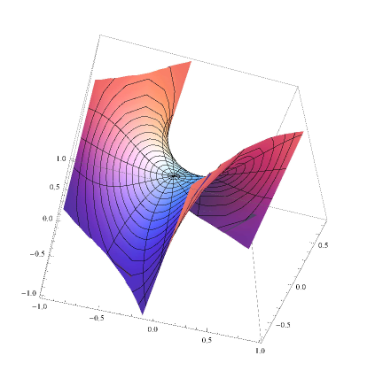
Figure 3.1. A Scherk type surface for $p=\pi/2+0.1$, $q=\pi-0.1$.

over the quadrilateral shown in Figure 3.2

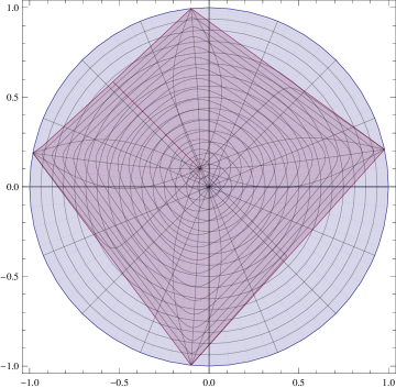
Figure 3.2. A bicentric quadrilateral inscribed in the unit disk for $p=\pi/2+0.1$, $q=\pi-0.1$.

4.  Curvature of two-parameter Scherk type surfaces and the proof of Theorem 1.5

After we gave the construction of two-parameter family of Scherk type surfaces, we continue with calculation of the curvature. It is given by

(4.1) $$\mathcal{K}=-\frac{4|\mathbf{q}^{\prime}|^{2}}{|\mathbf{p}|^{2}(1+|\mathbf{q}|^{2})^{4}}.$$

By using $|\mathbf{q}^{\prime}|=\frac{1-|a|^{2}}{|1-\overline{a}z|^{2}}$ and formulae (3.10), (3.11) and (3.22), we find that the Gaussian curvature at the point over the $0=f(z_{\circ})$ is equal to

(4.2) $$\mathcal{K}=-\frac{4(1-|a|^{2})^{2}}{|b|^{2}}\frac{|z_{\circ}^{2}-1|^{2}|z_{\circ}^{2}-e^{2\mathfrak{i}\alpha}|^{2}}{(|1-z_{\circ}\overline{a}|^{2}+|z_{\circ}-a|^{2})^{4}}.$$

Using already determined values of $a,b$ we get

(4.3) $$\begin{split}-\mathcal{K}&=\frac{4\pi^{2}(1+\sin p\sin(q-p))}{\left(1+\sqrt{\sin p\sin(q-p)}\right)^{4}}\frac{|1-z_{\circ}^{2}|^{2}|1-z_{\circ}^{2}e^{2\mathfrak{i}\alpha}|^{2}}{((1+|z_{\circ}|^{2})(1+|a|^{2})-4\Re(a\bar{z}_{\circ}))^{4}}\\ &=\frac{\pi^{2}}{4}\big{(}1+\sin p\sin(q-p)\big{)}\frac{|1-z_{\circ}^{2}|^{2}|1-z_{\circ}^{2}e^{2\mathfrak{i}\alpha}|^{2}}{((1+|z_{\circ}|^{2})-4\frac{\Re(a\bar{z}_{\circ})}{(1+|a|^{2})})^{4}}.\end{split}$$

Now our problem is reduced to maximization of the last expression for $(p,q)\in\mathcal{R}$. Note that $z_{\circ},$ $\alpha$ and $a$ also depend on $p,q.$ In order to prove the main inequality for the Gaussian curvature, next task will be localizing the zero of the mapping $f.$ It turns out that it is enough to find which one of four sectors $\{z:\arg z\in(0,\alpha)\},\{z:\arg z\in(\alpha,\pi)\},\{z:\arg z\in(\pi,\pi+\alpha)\}$ or $\{z:\arg z\in(\pi+\alpha,2\pi)\}$ contains the zero of $f.$

Let us show that that every sector is mapped by $f$ onto a curvilinear quadrilateral. Observe that the boundary function $G(t)=F(e^{it})$ of the harmonic function is piecewise continuous but has four jump discontinuities: $(t_{1},t_{2},t_{3},t_{4})=(0,\alpha,\pi,\pi+\alpha)$, $t_{5}=t_{1}+2\pi$. Moreover $G(0-)=e^{ip}$, $G(0+)=e^{ix}$, $G(\alpha-)=e^{ix}$, $G(\alpha+)=e^{iy}$, $G(\pi-)=e^{iy}$, $G(\pi+)=e^{is}$, $G(\pi+\alpha-)=e^{is}$, $G(\pi+\alpha+)=e^{ip}$.

Then

$$B_{k}=\lim_{r\to 1}f(re^{\mathfrak{i}t_{k}})=\frac{1}{2}\left(G(t_{k}-)+G(t_{k}+)\right),k=1,2,3,4,$$

and put $B_{5}=B_{1}$. Let $A_{1}=e^{\mathfrak{i}p}$, $A_{2}=e^{\mathfrak{i}x}$, $A_{3}=e^{\mathfrak{i}y}$, $A_{4}=e^{\mathfrak{i}s}$, $A_{5}=A_{1}$. This is a basic fact but we also refer to [4, p. 13].

Then the boundary of the first sector $\arg z\in[t_{k},t_{k+1}]$, $k=1,2,3,4$, consists of two curves $\gamma_{k}$, $\gamma_{k+1}$ ($\gamma_{5}=\gamma_{1}$) starting from $f(0)$ and emanating at the points $B_{k}$ and $B_{k+1}$ and the union of linear segments $B_{k}A_{k}$ and $A_{k}B_{k+1}$. The image of the sector $\arg z\in[t_{k},t_{k+1}]$ under $f$ is a domain $Q_{k}$, $k=1,2,3,4$ bounded by $\gamma_{k},$, $\gamma_{k+1}$, and $B_{k}A_{k}$ and $A_{k}B_{k+1}$. Observe that the quadrilateral $Q(e^{\mathfrak{i}p},e^{\mathfrak{i}x},e^{\mathfrak{i}y},e^{\mathfrak{i}s})$ is equal to $\bigcup_{k=1}^{4}Q_{k}$ (see Figure 4.1).

We will determine which of the domains $Q_{k}$, $k=1,2,3,4$ contains zero. In order to do so we consider the curves $\delta_{k}=\gamma_{k}+\gamma_{k+1}^{-}$, $k=1,2,3,4$, and find one that ”goes” around zero. Here superscript ”$-$” means that we have changed the orientation. The curve in co-domain ”goes around” the zero if and only if the field of its tangent vectors is monotonically decreasing or increasing, which indicates that it ”goes around” the zero in negative or positive direction. For a fixed pair $(p,q)$, there is exactly one sector that contains the zero $z_{\circ}$. We will determine it in the next lemma.

Lemma 4.1 (Localization of the zero $z_{\circ}$).

Assume that $(p,q)$ is a pair of real numbers that belongs to the domain $\mathcal{R}$ defined in (3.9) and assume that $z_{\circ}$ is the zero of $f$. Then we have

1. $\arg z_{\circ}\in(\alpha,\pi),$ for $q<\pi,q<2p,$

2. $\arg z_{\circ}\in(\pi+\alpha,2\pi),$ for $q>\pi,q>2p,$

3. $\arg z_{\circ}\in(\pi,\pi+\alpha),$ for $q\in(\pi,2p),$

4. $\arg z_{\circ}\in(0,\alpha)$, for $q\in(2p,\pi)$ .

The proof of Lemma 4.1 is presented in the following four subsections.

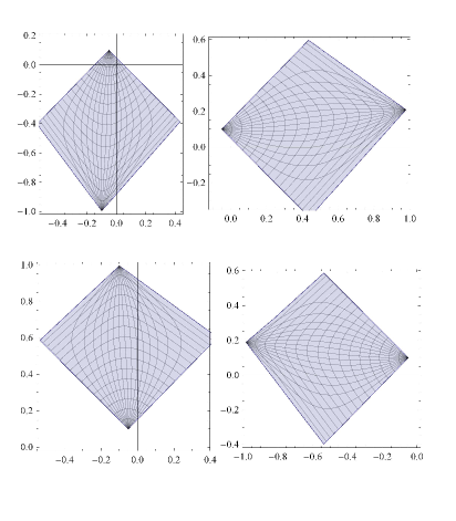
Figure 4.1. The images of four consecutive sectors, $\arg z\in[\alpha,\pi]$, $[\pi,\pi+\alpha]$, $[\pi+\alpha,2\pi]$ and $[0,\alpha]$ under the harmonic mapping $f$. In this case $p=\pi/2+0.1$, $q=\pi-0.1$, so $q<\min\{2p,\pi\}$. Notice that the first curvilinear quadrilateral contains the zero, and we are in the case a).

4.0.1.  The case a)

From the formulae for $u$ and $v$ ((3.13), (3.14)), we find:

$$\begin{split}u(re^{\mathfrak{i}\alpha})&=\frac{\cos p-\cos(p-q+2\beta)}{\pi}\tan^{-1}\frac{r\sin\alpha}{1+r\cos\alpha}\\ &+\frac{\cos(q-p+2\beta)-\cos p}{\pi}\tan^{-1}\frac{r\sin\alpha}{1-r\cos\alpha}\end{split}$$

and

$$\begin{split}v(re^{\mathfrak{i}\alpha})&=-\frac{\sin p+\sin(p-q+2\beta)}{\pi}\tan^{-1}\frac{r\sin\alpha}{1+r\cos\alpha}\\ &+\frac{\sin(q-p+2\beta)-\sin p}{\pi}\tan^{-1}\frac{r\sin\alpha}{1-r\cos\alpha},\end{split}$$

while

$$\begin{split}u(-r)&=\frac{\cos p-\cos(q-p+2\beta)}{\pi}\tan^{-1}\frac{r\sin\alpha}{1+r\cos\alpha}\\ &+\frac{\cos(p-q+2\beta)-\cos p}{\pi}\tan^{-1}\frac{r\sin\alpha}{1-r\cos\alpha}\end{split}$$

and

$$\begin{split}v(-r)&=-\frac{\sin p+\sin(q-p+2\beta)}{\pi}\tan^{-1}\frac{r\sin\alpha}{1+r\cos\alpha}\\ &+\frac{\sin(p-q+2\beta)-\sin p}{\pi}\tan^{-1}\frac{r\sin\alpha}{1-r\cos\alpha}.\end{split}$$

Now, we consider the following quantity:

$$\begin{split}\Psi(r,\varphi)&=\arg\bigg{(}\frac{\partial f(re^{\mathfrak{i}\varphi})}{\partial r}\bigg{)}\\ &=\arg\bigg{(}\frac{\partial u(re^{\mathfrak{i}\varphi})}{\partial r}+\mathfrak{i}\frac{\partial v(re^{\mathfrak{i}\varphi})}{\partial r}\bigg{)}\\ &=\tan^{-1}\bigg{(}\frac{\frac{\partial v(re^{\mathfrak{i}\varphi})}{\partial r}}{\frac{\partial u(re^{\mathfrak{i}\varphi})}{\partial r}}\bigg{)}.\end{split}$$

Its monotonicity gives an important property of the tangent vector at the curve $f(re^{\mathfrak{i}\varphi}),$ for fixed $\varphi$. In fact, the monotonicity of the argument of tangent vector means that the curve goes around $0,$ in one of two directions- positive if the function is increasing or negative if it is decreasing. Further, we have

$$\begin{split}\frac{\partial}{\partial r}u(re^{\mathfrak{i}\alpha})&=\frac{\cos p-\cos(p-q+2\beta)}{\pi}\frac{\sin\alpha}{1+r^{2}+2r\cos\alpha}\\ &+\frac{\cos(q-p+2\beta)-\cos p}{\pi}\frac{\sin\alpha}{1+r^{2}-2r\cos\alpha},\end{split}$$

$$\begin{split}\frac{\partial}{\partial r}v(re^{\mathfrak{i}\alpha})&=-\frac{\sin p+\sin(p-q+2\beta)}{\pi}\frac{\sin\alpha}{1+r^{2}+2r\cos\alpha}\\ &+\frac{\sin(q-p+2\beta)-\sin p}{\pi}\frac{\sin\alpha}{1+r^{2}-2r\cos\alpha}.\end{split}$$

The function $\Psi$ has the same monotonicity as the function $\tan\Psi,$ hence we will find the derivative of

$$\frac{\frac{\partial v(re^{\mathfrak{i}\varphi})}{\partial r}}{\frac{\partial u(re^{\mathfrak{i}\varphi})}{\partial r}}=\frac{P}{Q},$$

where

$$P=A(1+r^{2}+2r\cos\alpha)+B(1+r^{2}-2r\cos\alpha),$$

$$Q=C(1+r^{2}+2r\cos\alpha)+D(1+r^{2}-2r\cos\alpha),$$

with:

$$A=\sin(q-p+2\beta)-\sin p=2\sin(\frac{q}{2}-p+\beta)\cos(\beta+\frac{q}{2}),$$

$$B=-\sin p-\sin(p-q+2\beta)=-2\sin(p+\beta-\frac{q}{2})\cos(\frac{q}{2}-\beta),$$

$$C=\cos(q-p+2\beta)-\cos p=-2\sin(\beta+\frac{q}{2})\sin(\frac{q}{2}+\beta-p),$$

$$D=\cos p-\cos(p-q+2\beta)=-2\sin(p+\beta-\frac{q}{2})\sin(\beta-\frac{q}{2}).$$

The straightforward calculation gives

$$\begin{split}&P^{\prime}Q-Q^{\prime}P\\ &=\big{(}2A(r+\cos\alpha)+2B(r-\cos\alpha)\big{)}\bigg{(}C(1+r^{2}+2r\cos\alpha)+D(1+r^{2}-2r\cos\alpha)\bigg{)}\\ &-\big{(}2C(r+\cos\alpha)+2D(r-\cos\alpha)\big{)}\bigg{(}A(1+r^{2}+2r\cos\alpha)+B(1+r^{2}-2r\cos\alpha)\bigg{)}\\ &=4(1-r^{2})(AD-BC)\cos\alpha.\end{split}$$

For this range of $p$ and $q,$ we have $\cos\alpha=\frac{\tan(\frac{q}{2}-p)}{\tan\frac{q}{2}}\leq 0,$ since $0\leq\frac{q}{2}<\frac{\pi}{2}$ and $-\frac{\pi}{2}<\frac{q}{2}-p<0.$ Also,

$$\begin{split}AD-BC&=4\sin(\beta+\frac{q}{2}+\beta-p)\sin(\beta+p-\frac{q}{2})\\ &\times\bigg{(}-\sin(\beta-\frac{q}{2})\cos(\beta+\frac{q}{2})-\cos(\beta-\frac{q}{2})\sin(\beta+\frac{q}{2})\bigg{)}\\ &=-4\sin(\beta+\frac{q}{2}-p)\sin(\beta+p-\frac{q}{2})\sin(2\beta)<0,\end{split}$$

because $\beta+\frac{q}{2}-p,\beta+p-\frac{q}{2}\in(0,\pi)$ and $\beta\in(0,\frac{\pi}{2}).$

We conclude $P^{\prime}Q-Q^{\prime}P>0$, i.e. the tangent vector at $f(re^{\mathfrak{i}\alpha})$ has an increasing argument. (This follows from (3.4); it will be also important for the other cases.)

For the second part of the curve, we have:

$$\begin{split}\frac{\partial}{\partial r}u(-r)&=\frac{\cos p-\cos(q-p+2\beta)}{\pi}\frac{\sin\alpha}{1+r^{2}+2r\cos\alpha}\\ &+\frac{\cos(p-q+2\beta)-\cos p}{\pi}\frac{\sin\alpha}{1+r^{2}-2r\cos\alpha},\end{split}$$

$$\begin{split}\frac{\partial}{\partial r}v(-r)&=-\frac{\sin p+\sin(q-p+2\beta)}{\pi}\frac{\sin\alpha}{1+r^{2}+2r\cos\alpha}\\ &+\frac{\sin(p-q+2\beta)-\sin p}{\pi}\frac{\sin\alpha}{1+r^{2}-2r\cos\alpha}.\end{split}$$

This time, we consider

$$\tan\Psi=\frac{\frac{\partial}{\partial r}v(-r)}{\frac{\partial}{\partial r}u(-r)}=\frac{P}{Q}=\frac{A(1+r^{2}+2r\cos\alpha)+B(1+r^{2}-2r\cos\alpha}{C(1+r^{2}+2r\cos\alpha)+D(1+r^{2}-2r\cos\alpha)},$$

with:

$$A=\sin(p-q+2\beta)-\sin p=2\sin(\beta-\frac{q}{2})\cos(p+\beta-\frac{q}{2}),$$

$$B=-\sin p-\sin(q-p+2\beta)=-2\sin(\beta+\frac{q}{2})\cos(p-\beta-\frac{q}{2}),$$

$$C=\cos(p-q+2\beta)-\cos p=-2\sin(p+\beta-\frac{q}{2})\sin(\beta-\frac{q}{2}),$$

$$D=\cos p-\cos(q-p+2\beta)=-2\sin(\beta+\frac{q}{2})\sin(p-\beta-\frac{q}{2}).$$

Since we work on the same range of $p$’s and $q$’s, $\cos\alpha<0.$ Here we have:

$$\begin{split}AD-BC&=-4\sin(\beta+\frac{q}{2})\sin(\beta-\frac{q}{2})\\ &\times\bigg{(}\sin(p-\beta-\frac{q}{2})\cos(p+\beta-\frac{q}{2})+\cos(p-\beta-\frac{q}{2})\sin(p+\beta-\frac{q}{2})\bigg{)}\\ &=-4\sin(\beta+\frac{q}{2})\sin(\beta-\frac{q}{2})\sin(2p-q)>0,\end{split}$$

because $\frac{q}{2}-\beta\in(0,p),\beta+\frac{q}{2}\in(p,\pi)$ and $2p-q\in(0,\pi).$ This implies $P^{\prime}Q-Q^{\prime}P=4(1-r^{2})(AD-BC)\cos\alpha<0.$

Finally, we can conclude that the argument of the tangent vector of $f(re^{\mathfrak{i}\varphi})$ is increasing for $\varphi=\alpha$, while it is decreasing for $\alpha=\pi,$ considered as a function on $r.$ This exactly means that the whole curve, which consists of these two parts, which starts at $f(-1),$ goes as $f(-r)$ till $f(0)$ and then continues as $f(re^{i\alpha})$ till the end in $f(e^{\mathfrak{i}\alpha})$ has the tangent vector with an increasing argument i.e. it goes around the $0.$ This implies that $\arg z_{\circ}\in(\alpha,\pi).$

4.0.2.  The case b)

Let $q>\max\{\pi,2p\}.$ Here we consider $f(re^{\mathfrak{i}\varphi})$ with $\varphi=0$ and $\varphi=\pi+\alpha.$ We easily find that

$$\begin{split}\frac{\partial}{\partial r}u(r)&=\frac{\cos(q-p+2\beta)-\cos p}{\pi}\frac{\sin\alpha}{1+r^{2}-2r\cos\alpha}\\ &+\frac{\cos p-\cos(p-q+2\beta)}{\pi}\frac{\sin\alpha}{1+r^{2}+2r\cos\alpha},\end{split}$$

$$\begin{split}\frac{\partial}{\partial r}v(r)&=\frac{\sin(q-p+2\beta)+\sin p}{\pi}\frac{\sin\alpha}{1+r^{2}-2r\cos\alpha}\\ &+\frac{\sin p-\sin(p-q+2\beta)}{\pi}\frac{\sin\alpha}{1+r^{2}+2r\cos\alpha}\end{split}$$

and in the expression for

$$\tan\Psi=\frac{P}{Q}=\frac{A(1+r^{2}+2r\cos\alpha)+B(1+r^{2}-2r\cos\alpha)}{C(1+r^{2}+2r\cos\alpha)+D(1+r^{2}-2r\cos\alpha)},$$

we get:

$$A=\sin(q-p+2\beta)+\sin p=2\sin(\beta+\frac{q}{2})\cos(\beta+\frac{q}{2}-p),$$

$$B=\sin p-\sin(p-q+2\beta)=2\sin(\frac{q}{2}-\beta)\cos(p+\beta-\frac{q}{2}),$$

$$C=\cos(q-p+2\beta)-\cos p=-2\sin(\beta+\frac{q}{2})\sin(\frac{q}{2}+\beta-p),$$

$$D=\cos p-\cos(p-q+2\beta)=2\sin(\beta-\frac{q}{2})\sin(p+\beta-\frac{q}{2}).$$

For $q>\pi,q>2p$ we have $\cos\alpha=\frac{\tan(\frac{q}{2}-p)}{\tan\frac{q}{2}}<0,$ while:

$$\begin{split}AD-BC&=4\sin(\beta+\frac{q}{2})\sin(\beta-\frac{q}{2})\\ &\times\bigg{(}\sin(p+\beta-\frac{q}{2})\cos(\beta+\frac{q}{2}-p)-\sin(\frac{q}{2}+\beta-p)\cos(p+\beta-\frac{q}{2})\bigg{)}\\ &=4\sin(\beta+\frac{q}{2})\sin(\beta-\frac{q}{2})\sin(2p-q)>0.\end{split}$$

Therefore, $P^{\prime}Q-Q^{\prime}P=4(1-r^{2})(AD-BC)\cos\alpha<0.$

Similarly,

$$\frac{\partial}{\partial r}u(re^{\mathfrak{i}(\pi+\alpha)})=\frac{\cos(p-q+2\beta)-\cos p}{\pi}\frac{\sin\alpha}{1+r^{2}-2r\cos\alpha}$$

$$+\frac{\cos p-\cos(q-p+2\beta)}{\pi}\frac{\sin\alpha}{1+r^{2}+2r\cos\alpha},$$

$$\frac{\partial}{\partial r}v(re^{\mathfrak{i}(\pi+\alpha)})=\frac{\sin(p-q+2\beta)+\sin p}{\pi}\frac{\sin\alpha}{1+r^{2}-2r\cos\alpha}$$

$$+\frac{\sin p-\sin(q-p+2\beta)}{\pi}\frac{\sin\alpha}{1+r^{2}+2r\cos\alpha}$$

and for $\frac{P}{Q}$ we get the analogous expression, but with different values of the coefficients $(A,B,C,D)$:

$$A=\sin(p-q+2\beta)+\sin p=2\sin(p+\beta-\frac{q}{2})\cos(\frac{q}{2}-\beta),$$

$$B=\sin p-\sin(q-p+2\beta)=2\sin(p-\frac{q}{2}-\beta)\cos(\frac{q}{2}+\beta),$$

$$C=\cos(p-q+2\beta)-\cos p=-2\sin(p+\beta-\frac{q}{2})\sin(\beta-\frac{q}{2}),$$

$$D=\cos p-\cos(q-p+2\beta)=-2\sin(\beta+\frac{q}{2})\sin(p-\beta-\frac{q}{2}).$$

For this part of curve, we get:

$$\begin{split}AD-BC&=-4\sin(p-\beta-\frac{q}{2})\sin(p+\beta-\frac{q}{2})\\ &\times\bigg{(}-\sin(\beta+\frac{q}{2})\cos(\beta-\frac{q}{2})+\cos(\beta+\frac{q}{2})\sin(\beta-\frac{q}{2})\bigg{)}\\ &=-4\sin(p-\beta-\frac{q}{2})\sin(p+\beta-\frac{q}{2})\sin q<0,\end{split}$$

thus $P^{\prime}Q-Q^{\prime}P>0.$

The above calculations in this case allow us to conclude that the tangent vector of the curve, starting from $f(e^{\mathfrak{i}(\pi+\alpha)})$ and moving along $f(re^{\mathfrak{i}(\pi+\alpha)})$ through $f(0)$ and then along $f(r)$ ending in $f(1)$ has a decreasing argument, therefore $\arg z_{\circ}\in(\pi+\alpha,2\pi).$

4.0.3.  The case c), i.e. the case $q\in(\pi,2p)$

Proof of this case is similar. However, we will prove it using the earlier calculations. Namely in the previous cases, we already computed the coefficients $A,B,C,D$ for all $f(re^{\mathfrak{i}\varphi}),$ with $\varphi=0,\alpha,\pi,\pi+\alpha.$

For $\varphi=\pi,$ we have $AD-BC=-4\sin(\beta+\frac{q}{2})\sin(\beta-\frac{q}{2})\sin(2p-q)>0$ and $\cos\alpha>0,$ giving $P^{\prime}Q-Q^{\prime}P>0.$

On the other side, for $\varphi=\pi+\alpha,$ the same quantities are $AD-BC=-4\sin(p+\beta-\frac{q}{2})\sin(p-\beta-\frac{q}{2})\sin q<0$ and $\cos\alpha>0,$ which implies $P^{\prime}Q-Q^{\prime}P<0.$

We conclude now that the tangent vector of the curve starting from $f(-1)$ and moving along $f(-r)$ till $f(0)$ and then along $f(re^{\mathfrak{i}(\pi+\alpha)})$ till $f(e^{\mathfrak{i}(\pi+\alpha)})$ has a decreasing argument, hence $\arg z_{\circ}\in(\pi,\pi+\alpha).$

4.0.4.  The case d), i.e. $q\in(2p,\pi)$

For $\varphi=0,$ we get $AD-BC=4\sin(\beta+\frac{q}{2})\sin(\beta-\frac{q}{2})\sin(2p-q)>0$ and $\cos\alpha>0,$ which gives $P^{\prime}Q-Q^{\prime}P>0.$ The second part, i.e. for $\varphi=\alpha,$ $AD-BC=-4\sin(2\beta)\sin(\beta+\frac{q}{2}-p)\sin(\beta+p-\frac{q}{2})<0$ implies $P^{\prime}Q-Q^{\prime}P<0.$

The curve with starting point $f(1)$, crossing through the point $f(0)$ and ending in $f(e^{\mathfrak{i}\alpha})$ going along $f(r)$ and $f(re^{\mathfrak{i}\alpha})$, respectively, has an increasing argument. Thus $\arg z_{\circ}\in(0,\alpha).$

Proof of Theorem 1.5.

Given the Scherk type minimal surface $S:(u,v,\mathbf{f}(u,v))$ let $\tilde{f}$ be the projection of conformal parameterization (i.e. of Enneper–Weierstrass representation of the minimal graph $\varpi=(u,v,T):\mathbb{D}\to S\subset\mathbb{D}\times\mathbb{R}$). Then $\tilde{f}=(u,v)$ is a harmonic mapping of the unit disk onto $Q(b_{0},b_{1},b_{2},b_{3})$, which is certainly induced by a step mapping of the unit disk onto the vertices of the quadrilateral. Then there exists a unique Möbius transform $M$, which maps the points $1,e^{\mathfrak{i}\alpha},-1,-e^{\mathfrak{i}\alpha}$ onto the points $\tilde{f}^{-1}(b_{0},b_{1})$, $\tilde{f}^{-1}(b_{1},b_{2})$, $\tilde{f}^{-1}(b_{2},b_{3})$, $\tilde{f}^{-1}(b_{3},b_{0})$. Then the mapping $f=\tilde{f}\circ M$ satisfies the condition of Section 2. In other words we are in position to use constants $a$ and $z_{\circ}$, where $f(z_{\circ})=0$. Using Lemma 4.1 (the localization of $z_{\circ}=r_{0}e^{\mathfrak{i}t_{\circ}}$) and formulae for $a$ given by (3.23), (LABEL:eq:kosargumenta) and (LABEL:eq:sinargumenta), we find:

(4.4) $$\begin{split}\Re(z_{\circ}\overline{a})&=|z_{\circ}||a|\big{(}\cos t_{\circ}\cos\delta+\sin t_{\circ}\sin\delta\big{)}\\ \\ &=-\frac{|z_{\circ}||a|}{\sin\frac{q}{2}\sqrt{1-\sin p\sin(q-p)}}\\ &\times\bigg{(}\sin(\frac{q}{2}-p)\cos t_{\circ}+\cos\frac{q}{2}\sin t_{\circ}\sqrt{\sin p\sin(q-p)}\bigg{)}\leq 0.\end{split}$$

Indeed, for $q<\min\{\pi,2p\}$ we have $t_{\circ}\in(\alpha,\pi)$ and, since $\cos\alpha=\frac{\tan(\frac{q}{2}-p)}{\tan\frac{q}{2}}<0$ we conclude $t_{\circ}\in(\frac{\pi}{2},\pi)$ and $\sin t_{\circ}>0,\cos t_{\circ}<0.$ In this case, $\sin(\frac{q}{2}-p)<0$ and $\cos\frac{q}{2}>0$, hence the inequality follows.

Similarly, for $q>\max\{\pi,2p\}$ we have found that $t_{\circ}\in(\pi+\alpha,2\pi),$ and, by $\cos\alpha=\frac{\tan(\frac{q}{2}-p)}{\tan\frac{q}{2}}<0$ it follows that $t_{\circ}\in(\frac{3\pi}{2},2\pi)$ and $\sin t_{\circ}<0,\cos t_{\circ}>0.$ Also, $\sin(\frac{q}{2}-p)>0$ and $\cos\frac{q}{2}<0$ and we are done again.

The same reasoning works for the two remaining cases. If $q\in(\pi,2p)$ then $t_{\circ}\in(\pi,\pi+\alpha),$ while $\cos\alpha=\frac{\tan(\frac{q}{2}-p)}{\tan\frac{q}{2}}>0$ gives $\alpha\in(0,\frac{\pi}{2})$ and $t_{\circ}\in(\pi,\frac{3\pi}{2})$, thus $\sin t_{\circ}<0,\cos t_{\circ}<0.$ Now, $\sin(\frac{q}{2}-p)<0$ and $\cos\frac{q}{2}<0$ implies the non-positivity of $\Re(z_{\circ}\overline{a}).$ If $q\in(2p,\pi)$ then $t_{\circ}\in(0,\alpha),$ with $\cos\alpha=\frac{\tan(\frac{q}{2}-p)}{\tan\frac{q}{2}}>0$ which leads to $t_{\circ}\in(0,\frac{\pi}{2})$ and $\sin t_{\circ}>0$ and $\cos t_{\circ}>0.$ The conclusion follows from $\sin(\frac{q}{2}-p)>0$ and $\cos\frac{q}{2}>0.$

By using continuity and limiting process we can conclude the same for $q=2p$ or $q=\pi.$ The reader can note that in these two cases, one of two summands from the brackets in (4.4) is equal to zero, while the other is non-negative. Only for $p=\frac{\pi}{2}$ and $q=\pi,$ both of them are $0$ and $\Re(z_{\circ}\overline{a})=0.$ Also, for $q=2p$ we have $e^{\mathfrak{i}p}e^{\mathfrak{i}s}=e^{\mathfrak{i}x}e^{\mathfrak{i}y},$ which means that the quadrilateral in the co-domain is a trapezoid. Similarly, for $q=\pi$ there holds $e^{\mathfrak{i}p}e^{\mathfrak{i}x}=e^{\mathfrak{i}y}e^{\mathfrak{i}s},$ and the image is again a trapezoid. The case of the deltoid as the image has been mentioned in [16], but without a proof. Here, it is covered when $q-p=\frac{\pi}{2}.$

From the formula (4.3) we get

$$|\mathcal{K}|\leq\frac{\pi^{2}}{2}\frac{|1-z_{\circ}^{2}|^{2}|z_{\circ}^{2}-e^{2\mathfrak{i}\alpha}|^{2}}{(1+|z_{\circ}|^{2})^{4}}\leq\frac{\pi^{2}}{2},$$

which was to be proved. ∎

Acknowledgements

The first author is partially supported by a research fund of University of Montenegro. The authors would like to thank Franc Forstnerič for fruitful conversation and his remarks which led to improved presentation and he also thanks Antonio Ros for encouraging him to work on this problem. We also wish to thank the following people for a number of useful remarks that have improved the presentation of this paper Kristian Seip, Anti Perälä and Igor Uljarević. The second author is partially supported by MPNTR grant, no. 174017, Serbia.

David Kalaj

University of Montenegro, Faculty of Natural Sciences and Mathematics, 81000, Podgorica, Montenegro

e-mail: davidk@ucg.ac.me

Petar Melentijević

University of Belgrade, Faculty of Mathematics, 11000, Belgrade, Serbia,

e-mail: petarmel@matf.bg.ac.rs

References

- [1] A. Alarcon, F. Forstnerič, F. J. Lopez, Minimal surfaces from a complex analytic viewpoint, Springer Monographs in Mathematics, Springer, Cham, (2021)
- [2] D. Bshouty, A. Lyzzaik, A. Weitsman, Uniqueness of Harmonic Mappings with Blaschke Dilatations, J. Geom. Anal., 17(1):41-47, (2007)
- [3] T. H. Colding and W. P. I. Minicozzi. A course in minimal surfaces, volume 121. Providence, RI: American Mathematical Society (AMS), 2011.
- [4] P. Duren, Harmonic mappings in the plane, volume 156 of Cambridge Tracts in Mathematics, Cambridge University Press, Cambridge, (2004)
- [5] S. Finch, Mathematical constants II, Encyclopedia of Mathematics and its Applications, Cambridge University Press, (2018)
- [6] R. Finn and R. Osserman, On the Gauss curvature of non-parametric minimal surfaces, J. Analyse Math., 12:351-364, (1964)
- [7] R. R. Hall, On an inequality of E. Heinz, J. Analyse Math., 42:185-198, (1982/83)
- [8] R. R. Hall, The Gaussian curvature of minimal surfaces and Heinz’ constant, J. Reine. Angew. Math., 502:19-28, (1998)
- [9] E. Heinz, Über die Lösungen der Minimalflächengleichung, Nachr. Acad. Wiss. Göttingen, Math.-Phys. Kl., Math.-Phys.-Chem. Abt., 44:51-56, (1952)
- [10] W. Hengartner, G. Schober, Harmonic mappings with given dilatation, J. London Math. Soc.(2), 33(3):473-483, (1986)
- [11] E. Hopf, On an inequality for minimal surfaces , J. Ration. Mech. Anal., 2:519-522, (1953)
- [12] H. Jenkins, J. Serrin, Variational problems of minimal surface type. III: The Dirichlet problem with infinite data, Arch. Ration. Mech. Anal., 29:304-322, (1968)
- [13] D. Kalaj, Curvature of minimal graphs, arXiv 2108.09447
- [14] L. V. Kovalev and X. Yang. Fourier series of circle embeddings. Comput. Methods Funct. Theory, 19(2):323–340, 2019.
- [15] J. C. C. Nitsche, On new results in the theory of minimal surfaces, Bull. Amer. Math. Soc., 71:195-270, (1965)
- [16] J. C. C. Nitsche, On the inequality of E. Heinz and E. Hopf, Appl. Anal., 3:47-56, (1973)
- [17] T. Sheil-Small, On the Fourier Series of a Step Function, Michigan Math. J., 36(3):459-475, (1989)