Worldvolume tempered Lefschetz thimble method and its error estimation

Abstract

The worldvolume tempered Lefschetz thimble method (WV-TLTM) is an algorithm towards solving the sign problem, where hybrid Monte Carlo updates are performed on a continuous accumulation of flowed surfaces foliated by the anti-holomorphic gradient flow (the worldvolume of integration surface). Sharing the advantage with the original tempered Lefschetz thimble method (TLTM) that the sign problem is resolved without introducing the ergodicity problem, the new algorithm is expected to significantly reduce the computational cost, because it eliminates the need to compute the Jacobian of the flow in generating a configuration. We demonstrate the effectiveness of the WV-TLTM with its successful application to the Stephanov model (a chiral random matrix model), for which the complex Langevin method is known to suffer from a serious wrong convergence problem. We also discuss the statistical analysis method for the WV-TLTM.

1 Introduction

The sign problem is a notorious problem in applying Monte Carlo methods to systems with complex actions, which include the finite density QCD as a typical example [1]. The tempered Lefschetz thimble method (TLTM) [2] was proposed as a versatile solution to this problem. This algorithm resolves the ergodicity problem inherent in Lefschetz thimble methods by tempering the system with the antiholomorphic gradient flow, where a discrete set of replicas of configuration space is introduced. In spite of its successful applications to various models [2, 3, 4], the original TLTM has a drawback of high computational costs in generating a configuration, coming from the calculation of the Jacobian of the flow and from the introduction of a large number of replicas to ensure a sufficiently large acceptance rate in exchanging configurations between adjacent replicas.

The worldvolume tempered Lefschetz thimble method (WV-TLTM) [5] was introduced to overcome this issue. This algorithm belongs to a class of worldvolume Hybrid Monte Carlo (WV-HMC), where HMC updates are performed on a continuous set of replicas (the worldvolume of integration surface). The WV-TLTM is expected to significantly reduce the computational costs, because one no longer needs to compute the Jacobian of the flow in generating a configuration. In this talk, we review the WV-TLTM and show its successful application [5] to the Stephanov model [6]. We also discuss the statistical analysis method for this algorithm [7]. The basics and other applications of the (WV-)TLTM are discussed in the contribution [8].

2 Worldvolume tempered Lefschetz thimble method

In the Lefschetz thimble method [9, 10, 11, 12], we complexify the integration variable from $x\in{\mathbb{R}}^{N}$ to $z=x+iy\in{\mathbb{C}}^{N}$. We assume that the integrands in path integrals are entire functions over ${\mathbb{C}^{N}}$. Then, Cauchy’s theorem ensures that the integration surface can be continuously deformed, $\Sigma_{0}={\mathbb{R}^{N}}\to\Sigma_{t}$ ($t$ : deformation parameter), without changing the values of the integrals:

$$\langle{\mathcal{O}}\rangle\equiv\frac{\int_{{\mathbb{R}^{N}}}dx\,e^{-S(x)}{\mathcal{O}}(x)}{\int_{{\mathbb{R}^{N}}}dx\,e^{-S(x)}}=\frac{\int_{{\Sigma_{t}}}dz_{t}\,e^{-S(z_{t})}\mathcal{O}(z_{t})}{\int_{{\Sigma_{t}}}dz_{t}\,e^{-S(z_{t})}}.$$ (1)

We deform the integration surface with the following anti-holomorphic gradient flow:

$$\frac{d}{dt}z_{t}=[\partial S(z_{t})]^{*},\quad z_{t=0}=x.$$ (2)

The crucial property of the flow is that the flowed surface approaches a union of Lefschetz thimbles:

$${\Sigma_{t}}\xrightarrow{t\to\infty}\bigcup_{\sigma}{\mathcal{J}}_{\sigma},$$ (3)

where the Lefschetz thimble ${\mathcal{J}}_{\sigma}$ associated with a critical point $z_{\sigma}$ [at which $\partial S(z_{\sigma})=0$] consists of orbits flowing out of $z_{\sigma}$. Since the imaginary part of the action is constant on each ${\mathcal{J}}_{\sigma}$ [${\rm Im}\,S(z)={\rm Im}\,S(z_{\sigma})$ $(z\in{\mathcal{J}}_{\sigma})$], the oscillatory behavior of the integrals will become mild at large $t$. However, multiple ${\mathcal{J}}_{\sigma}$’s are often relevant to the estimation of the path integral [13], and since ${\mathcal{J}}_{\sigma}$’s are separated by regions where ${\rm Re}\,S(z)=\infty$, the distribution on $\Sigma_{t}$ gets multimodal as we increase the flow time $t$.

The tempered Lefschetz thimble method (TLTM) [2] resolves this issue by tempering the system with the flow time (where the parallel tempering [14, 15, 16] is employed). However, this algorithm becomes expensive at large degrees of freedom because of the increasing number of replicas so as to ensure a sufficiently large acceptance rate in the exchange process, as well as of the calculation of the determinant of the Jacobian of the flow, $J_{t}(x)\equiv\partial z_{t}(x)/\partial x$.

The worldvolume tempered Lefschetz thimble method (WV-TLTM) [5] resolves this drawback of the original TLTM. The key observation in the new algorithm is that Eq. (1) can be expressed as an integral over a region

$${\mathcal{R}}\equiv\bigl{\{}z_{t}(x)\in{\mathbb{C}}^{N}\,\bigl{|}\,\,x\in{\mathbb{R}^{N}},\,t\in[T_{0},T_{1}]\bigr{\}}=\bigcup_{t=T_{0}}^{T_{1}}{\Sigma_{t}},$$ (4)

by averaging the numerator and the denominator in Eq. (1) over $t$ with an arbitrary weight $e^{-W(t)}$:

$$\langle{\mathcal{O}}\rangle=\frac{\int_{{\Sigma_{t}}}dz_{t}\,e^{-S(z_{t})}\mathcal{O}(z_{t})}{\int_{{\Sigma_{t}}}dz_{t}\,e^{-S(z_{t})}}=\frac{\int_{T_{0}}^{T_{1}}dt\,e^{-W(t)}\int_{{\Sigma_{t}}}dz_{t}\,e^{-S(z_{t})}\mathcal{O}(z_{t})}{\int_{T_{0}}^{T_{1}}dt\,e^{-W(t)}\int_{{\Sigma_{t}}}dz_{t}\,e^{-S(z_{t})}}.$$ (5)

We call the region ${\mathcal{R}}$ the worldvolume, because this can be regarded as an orbit of integration surface (see Fig. 1).

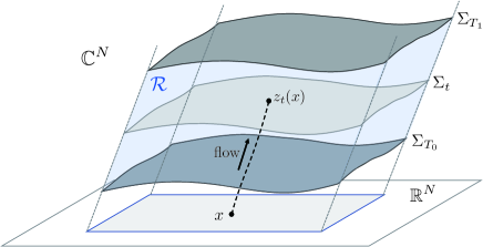
Figure 1: The worldvolume ${\mathcal{R}}$ (colored region) consisting of ${\Sigma_{t}}$ foliated by the flow (2) .

To perform Monte Carlo calculations, we further rewrite Eq. (5) to the form

$$\langle{\mathcal{O}}\rangle=\frac{\int_{{\mathcal{R}}}Dz\,e^{-[W(t(z))+{\rm Re}\,S(z)]}\bigl{(}dt\,dz_{t}/Dz\bigr{)}\,e^{-i\,{\rm Im}\,S(z)}\,\mathcal{O}(z)}{\int_{{\mathcal{R}}}Dz\,e^{-[W(t(z))+{\rm Re}\,S(z)]}\bigl{(}dt\,dz_{t}/Dz\bigr{)}\,e^{-i\,{\rm Im}\,S(z)}},$$ (6)

where $Dz$ is the invariant volume element on ${\mathcal{R}}$ and $t(z)$ is the flow time at $z\in{\mathcal{R}}$. If we use $(t,x)$ as coordinates on ${\mathcal{R}}$, then $dz_{t}$ and $Dz$ can be written as

$$dz_{t} =\det J_{t}(x)\,dx,$$ (7)

$$Dz =\alpha(z_{t}(x))\,|\det J_{t}(x)|\,dx\,dt,$$ (8)

where $\alpha(z_{t})$ is the magnitude of the normal component of $\dot{z}_{t}(x)=[\partial S(z_{t}(x))]^{\ast}$ to ${\mathcal{R}}$. Then, by introducing the potential $V(z)$ and the reweighting factor $A(z)$ as

$$V(z) \equiv{\rm Re}\,S(z)+W(t(z)),$$ (9)

$$A(z) \equiv\frac{dtdz_{t}}{Dz}\,e^{-i\,{\rm Im}\,S(z)}=\alpha^{-1}(z)\,\frac{\det\,J_{t}(x)}{|\det\,J_{t}(x)|}\,e^{-i\,{\rm Im}\,S(z)},$$ (10)

Eq. (6) can be written as a ratio of reweighted averages,

$$\langle{\mathcal{O}}\rangle=\frac{\langle A(z)\,{\mathcal{O}}(z)\rangle_{\mathcal{R}}}{\langle A(z)\rangle_{\mathcal{R}}}\quad\biggl{(}\langle f(z)\rangle_{\mathcal{R}}\equiv\frac{\int_{{\mathcal{R}}}Dz\,e^{-V(z)}f(z)}{\int_{{\mathcal{R}}}Dz\,e^{-V(z)}}\biggr{)}.$$ (11)

The reweighted averages $\langle\,\ast\,\rangle_{\mathcal{R}}$ on the subspace ${\mathcal{R}}$ are estimated by the Hybrid Monte Carlo with the RATTLE discretization [17, 18] (for the use of the RATTLE in Lefschetz thimble methods, see [11, 19] and [4]).

The computational cost of the WV-TLTM is reduced from that of the original TLTM for two reasons. One is that the continuous migration of $t$ eliminates the need to worry about the acceptance rate in the exchange process. The other is that, as the potential $V(z)$ in the molecular dynamics does not contain the Jacobian matrix $J_{t}(x)$ [see Eq. (9)], $J_{t}(x)$ needs not be calculated in generating a configuration if we use an iterative method in linear inversion as in Ref. [20] (see Ref. [5] for details).

3 Application to the Stephanov model

To confirm the effectiveness of the WV-TLTM, we apply this algorithm to the Stephanov model [6]. This model has been regarded as an important benchmark for algorithms towards solving the sign problem, because it reproduces the qualitative behavior of finite density QCD in the limit of large matrix size [22, 6, 21] and also it gives rise to a serious wrong convergence problem [23] with the complex Langevin method [24, 25].

The partition function of the model is given by

$$Z_{\rm Steph}\equiv\int d^{2}We^{-n\,{\rm tr}\,W^{\dagger}W}{\rm det}\begin{bmatrix}m&iW+\mu\\ iW^{\dagger}+\mu&m\\ \end{bmatrix}.$$ (12)

Here, $W$ is an $n\times n$ complex matrix representing the gauge-field degrees of freedom with a flat measure $d^{2}W\equiv\prod_{i,j}(d{\rm Re}\,W_{ij}\,d{\rm Im}\,W_{ij})$, and $m$ and $\mu$ correspond to the quark mass and the baryon number chemical potential, respectively. We have set the temperature to zero, for which the sign problem is most severe. We estimate the chiral condensate $\langle\overline{\psi}\psi\rangle$ and the baryon number density $\langle\psi^{\dagger}\psi\rangle$ defined by

$$\langle\overline{\psi}\psi\rangle\equiv\frac{1}{2n}\,\frac{\partial}{\partial m}\log Z_{\rm Steph},\quad\langle\psi^{\dagger}\psi\rangle\equiv\frac{1}{2n}\,\frac{\partial}{\partial\mu}\log Z_{\rm Steph}.$$ (13)

Figure 2 shows the results for varying $\mu$ with $n=10$ (thus $N=2n^{2}=200$) and $m=0.004$.

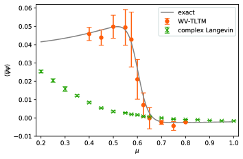
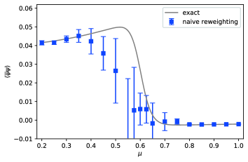
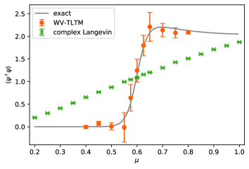
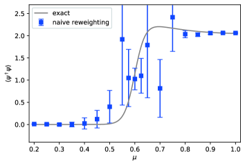
Figure 2: Estimates of the chiral condensate (upper panels) and the number density (lower panels) [5].

We also give for comparison the results obtained with the naive reweighting method and with the complex Langevin method (see [5] for detailed analysis). This size of matrix ($n=10$) requires more than about 70 replicas in the original TLTM, making the computation very costly. The sample size is set to 4,000–17,000 for the WV-TLTM varying on $\mu$, and to 10,000 for the naive reweighting and complex Langevin methods.

From the results with the naive reweighting, we see that there is a severe sign problem for this parameter. We also see that the complex Langevin suffers from the wrong convergence (largely deviated means from the exact values with small statistical errors; see [23] for a detailed analysis of the Stephanov model with the complex Langevin method). In contrast, the WV-TLTM gives results in good agreement with the exact values with controlled statistical errors, which proves the effectiveness of the WV-TLTM.

4 Statistical analysis method for the WV-TLTM

In generating configurations, $T_{1}$ must be set sufficiently large to reduce the sign problem and $T_{0}$ sufficiently small to recover ergodicity. In the estimation, however, we can use different values of $T_{0},\,T_{1}$ (denoted by $\tilde{T}_{0}$,  $\tilde{T}_{1}$) by restricting the data to those belonging to the interval $[\tilde{T}_{0},\tilde{T}_{1}]$. Note that in an ideal situation the estimate of a fixed observable does not depend on the choice of $\tilde{T}_{0},\,\tilde{T}_{1}$ according to Cauchy’s theorem. We can in turn use this fact in actual calculations to test the sufficiency of the sample size for the whole configuration space to be well explored. Furthermore, when necessary, we may exclude two extreme regions: one is the small $t$ region suffering from phase fluctuations, and the other is the large $t$ region having possible large autocorrelations and systematic errors due to the complicated geometry of $\Sigma_{t}$ at large $t$.

We now show that the restricted data set can be regarded as obtained from a Markov chain [7]. Let $P(z^{\prime}|z)$ be the transition matrix in the whole worldvolume with $[T_{0},T_{1}]$, and denote by $\tilde{\mathcal{R}}$ the restricted region with $[\tilde{T}_{0}$, $\tilde{T}_{1}]$. Then, the probability $\tilde{P}(z^{\prime}|z)$ to obtain $z^{\prime}\in\tilde{\mathcal{R}}$ from $z\in\tilde{\mathcal{R}}$ can be expressed as

$$\tilde{P}(z^{\prime}|z)=P(z^{\prime}|z)+\int_{{\tilde{\mathcal{R}}}^{c}}dw\,P(z^{\prime}|w)P(w|z)+\int_{{\tilde{\mathcal{R}}}^{c}}dw_{2}dw_{1}\,P(z^{\prime}|w_{2})P(w_{2}|w_{1})P(w_{1}|z)+\cdots,$$ (14)

where $\tilde{{\mathcal{R}}}^{c}\equiv{\mathcal{R}}\backslash\tilde{{\mathcal{R}}}$. The first term describes a direct transition in $\tilde{{\mathcal{R}}}$, while the rest describes processes that leave $\tilde{\mathcal{R}}$ once. The ergodicity of $P$ ensures that of $\tilde{P}$, so that $\tilde{P}$ has the correct normalization as a transition matrix. Furthermore, if $P$ satisfies the detailed balance with equilibrium distribution $\rho_{\rm eq}(z)$, $\tilde{P}$ also satisfies the detailed balance with the equilibrium distribution $\tilde{\rho}_{\rm eq}(z)\equiv\rho_{\rm eq}(z)/\int_{\tilde{\mathcal{R}}}dz\,\rho_{\rm eq}(z)$. We thus can apply standard statistical analysis methods (such as the Jackknife) to the restricted data set.

Figure 3 shows the estimates of the baryon number density with varying $\tilde{T}_{0}$ and fixed $\tilde{T}_{1}$ for the Stephanov model of a matrix size $n=2$ (see [7] for details). We observe a plateau for a wide range of $r\equiv(\tilde{T}_{1}-\tilde{T}_{0})/(T_{1}-T_{0})$, from which we confirm that the estimates do not depend on $\tilde{T}_{0}$. The estimates are slightly deviated from the exact value at $r\lesssim 0.2$, but this can be understood by the smallness of the sample size when $\tilde{T}_{0}$ gets close to $\tilde{T}_{1}$.

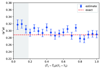
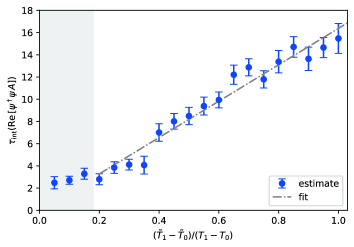
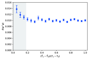
Figure 3: The dependence of statistical quantities on the choice of $\tilde{\mathcal{R}}$ with varying $\tilde{T}_{0}$ and fixed $\tilde{T}_{1}$. (Top) $\tilde{T}_{0}$-independence of the estimates [7]. (Bottom left) Scaling of $\tilde{\tau}_{{\rm int}}$, Eq. (18), and (Bottom right) $\tilde{T}_{0}$-independence of the statistical errors, Eq. (20) [7]. The integrated autocorrelation times are saturated in the shaded region, $\tilde{\tau}_{{\rm int}}\simeq 1$, where the scaling (18) breaks down.

One may be worried about the increase in statistical errors due to the reduced size of restricted data set. We can argue that this is not the case because the effect of the decrease in the sample size is compensated by the decrease in autocorrelation. In fact, one can show that the effective sample size $N_{\rm conf}^{\rm eff}$ defined by

$$N_{\rm conf}^{\rm eff}\equiv N_{\rm conf}/\tau_{\rm int}$$ (15)

does not depend on the choice of $\tilde{T}_{0},\,\tilde{T}_{1}$. Here, $N_{\rm conf}$ is the original sample size, and $\tau_{\rm int}$ is the integrated autocorrelation time of a given operator ${\mathcal{O}}$, defined from the autocorrelation functions $C_{k}\equiv\langle(\mathcal{O}_{0}-\langle\mathcal{O}\rangle)(\mathcal{O}_{k}-\langle\mathcal{O}\rangle)\rangle$ as

$$\tau_{\rm int}\equiv 1+2\sum_{k=1}^{\infty}C_{k}/C_{0}.$$ (16)

We assume that the flow time $t\in[T_{0},T_{1}]$ is uniformly distributed, which is equivalent to assuming that the weight function $W(t)$ is ideally chosen [see discussion below Eq. (5)]. We also assume that the integrated autocorrelation time of $t$ is 1. Then, the probability for a configuration to appear in $[\tilde{T}_{0},\tilde{T}_{1}]$ is given by

$$p\equiv\frac{\tilde{T}_{1}-\tilde{T}_{0}}{T_{1}-T_{0}}.$$ (17)

Since a configuration appears in the subregion $\tilde{{\mathcal{R}}}$ with this probability, the integrated autocorrelation time of the subsample will be reduced as

$$\tilde{\tau}_{\rm int}=p\tau_{\rm int}.$$ (18)

Since the sample size is reduced with the same ratio, $\tilde{N}_{\rm conf}=pN_{\rm conf}$, the effective sample size does not change:

$$\tilde{N}_{\rm conf}/\tilde{\tau}_{\rm int}=N_{\rm conf}/\tau_{\rm int}=N_{\rm conf}^{\rm eff},$$ (19)

which means that the statistical error $\delta\langle{\mathcal{O}}\rangle$ to the estimate of $\langle\mathcal{O}\rangle$ is independent of the choice of $\tilde{T}_{0},\tilde{T}_{1}$ because $\delta\langle{\mathcal{O}}\rangle$ is given by the formula

$$\delta\langle{\mathcal{O}}\rangle=\sigma_{{\mathcal{O}}}/\sqrt{N_{\rm conf}^{\rm eff}}\quad\bigl{(}\sigma_{{\mathcal{O}}}^{2}\equiv\langle({\mathcal{O}}-\langle{\mathcal{O}}\rangle)^{2}\rangle\bigr{)}.$$ (20)

The scaling (18) and the $\tilde{T}_{0},\tilde{T}_{1}$-independence of Eq. (20) can actually be confirmed as in Fig. 3.

5 Summary and outlook

We have reported that the worldvolume tempered Lefschetz thimble method (WV-TLTM) works quite well, by demonstrating its effectiveness with the application to the Stephanov model. We also discussed the statistical analysis method for the WV-TLTM, which is expected to become useful especially when performing large-scale computations.

We are now preparing large-scale simulations with the WV-TLTM for systems having the sign problem, such as finite density QCD, the Hubbard model, and real-time QM/QFTs. In parallel with research in this direction, we believe that it is still important to continue developing the algorithm itself, for example, to find an efficient algorithm to determine the weight function $W(t)$. A study along these lines is in progress and will be reported elsewhere.

References

- [1] J. Guenther, An overview of the QCD phase diagram at finite and , PoS LATTICE2021 (2021) 013
- [2] M. Fukuma and N. Umeda, Parallel tempering algorithm for integration over Lefschetz thimbles, PTEP 2017 (2017) 073B01 [hep-lat/1703.00861].
- [3] M. Fukuma, N. Matsumoto and N. Umeda, Applying the tempered Lefschetz thimble method to the Hubbard model away from half filling, Phys. Rev. D 100 (2019) 114510 [1906.04243].
- [4] M. Fukuma, N. Matsumoto and N. Umeda, Implementation of the HMC algorithm on the tempered Lefschetz thimble method, 1912.13303.
- [5] M. Fukuma and N. Matsumoto, Worldvolume approach to the tempered Lefschetz thimble method, PTEP 2021 (2021) 023B08 [2012.08468].
- [6] M. A. Stephanov, Random matrix model of QCD at finite density and the nature of the quenched limit, Phys. Rev. Lett. 76 (1996) 4472 [hep-lat/9604003].
- [7] M. Fukuma, N. Matsumoto and Y. Namekawa, Statistical analysis method for the worldvolume hybrid Monte Carlo algorithm, to appear in PTEP [hep-lat/2107.06858].
- [8] M. Fukuma, N. Matsumoto, The basics and applications of the tempered Lefschetz thimble method for the numerical sign problem, PoS LATTICE2021 (2021) 395.
- [9] E. Witten, Analytic Continuation Of Chern-Simons Theory, AMS/IP Stud. Adv. Math. 50 (2011) 347 [1001.2933].
- [10] M. Cristoforetti, F. Di Renzo and L. Scorzato, New approach to the sign problem in quantum field theories: High density QCD on a Lefschetz thimble, Phys. Rev. D 86 (2012) 074506 [1205.3996].
- [11] H. Fujii, D. Honda, M. Kato, Y. Kikukawa, S. Komatsu and T. Sano, Hybrid Monte Carlo on Lefschetz thimbles - A study of the residual sign problem, JHEP 1310 (2013) 147 [1309.4371].
- [12] A. Alexandru, G. Başar, P. F. Bedaque, G. W. Ridgway and N. C. Warrington, Sign problem and Monte Carlo calculations beyond Lefschetz thimbles, JHEP 1605 (2016) 053 [hep-lat/1512.08764].
- [13] H. Fujii, S. Kamata and Y. Kikukawa, Lefschetz thimble structure in one-dimensional lattice Thirring model at finite density, JHEP 11 (2015) 078 [erratum: JHEP 02 (2016) 036] [hep-lat/1509.08176].
- [14] R. H. Swendsen and J.-S. Wang, Replica Monte Carlo Simulation of Spin-Glasses, Phys. Rev. Lett. 57 (1986) 2607.
- [15] C. J. Geyer, Markov Chain Monte Carlo Maximum Likelihood, in Computing Science and Statistics: Proceedings of the 23rd Symposium on the Interface, American Statistical Association, New York, p. 156 (1991).
- [16] K. Hukushima and K. Nemoto, Exchange Monte Carlo method and application to spin glass simulations, J. Phys. Soc. Jpn. 65 (1996) 1604.
- [17] H. C. Andersen, RATTLE: A “velocity” version of the SHAKE algorithm for molecular dynamics calculations, J. Comput. Phys. 52 (1983) 24.
- [18] B. J. Leimkuhler and R. D. Skeel, Symplectic numerical integrators in constrained Hamiltonian systems, J. Comput. Phys. 112 (1994) 117 .
- [19] A. Alexandru, Improved algorithms for generalized thimble method, talk at the 37th international conference on lattice field theory, Wuhan, 2019.
- [20] A. Alexandru, G. Başar, P. F. Bedaque and G. W. Ridgway, Schwinger-Keldysh formalism on the lattice: A faster algorithm and its application to field theory, Phys. Rev. D 95 (2017) 114501 [1704.06404].
- [21] M. A. Halasz, A. D. Jackson, R. E. Shrock, M. A. Stephanov and J. J. M. Verbaarschot, On the phase diagram of QCD, Phys. Rev. D 58 (1998) 096007 [hep-ph/9804290].
- [22] E. V. Shuryak and J. J. M. Verbaarschot, Random matrix theory and spectral sum rules for the Dirac operator in QCD, Nucl. Phys. A 560 (1993) 306-320 [hep-th/9212088].
- [23] J. Bloch, J. Glesaaen, J. J. M. Verbaarschot and S. Zafeiropoulos, Complex Langevin Simulation of a Random Matrix Model at Nonzero Chemical Potential, JHEP 03 (2018) 015 [1712.07514].
- [24] G. Parisi, On complex probabilities, Phys. Lett. B 131 (1983) 393.
- [25] J.R. Klauder, Coherent State Langevin Equations for Canonical Quantum Systems With Applications to the Quantized Hall Effect, Phys. Rev. A 29 (1984) 2036.