Chaos and irreversibility of a flexible filament in periodically–driven Stokes flow

Abstract

The flow of Newtonian fluid at low Reynolds number is, in general, regular and time-reversible due to absence of nonlinear effects. For example, if the fluid is sheared by its boundary motion that is subsequently reversed, then all the fluid elements return to their initial positions. Consequently, mixing in microchannels happens solely due to molecular diffusion and is very slow. Here, we show, numerically, that the introduction of a single, freely-floating, flexible filament in a time-periodic linear shear flow can break reversibility and give rise to chaos due to elastic nonlinearities, if the bending rigidity of the filament is within a carefully chosen range. Within this range, not only the shape of the filament is spatiotemporally chaotic, but also the flow is an efficient mixer. Overall, we find five dynamical phases: the shape of a stiff filament is time-invariant – either straight or buckled; it undergoes a period-two bifurcation as the filament is made softer; becomes spatiotemporally chaotic for even softer filaments but, surprisingly, the chaos is suppressed if bending rigidity is decreased further.

I Introduction

Flows at very small Reynolds number play a key role in biology Purcell (1977); Lauga and Powers (2009); Phillips et al. (2012); Taylor (1951) and microfluidics Squires and Quake (2005); Kirby (2010); Stone et al. (2004). In the presence of rigid boundaries, such flows are typically laminar and reversible. For example, consider the fluid between two concentric cylinders sheared by rotating the outer one slowly. If the rotation is reversed the fluid particles come back to their original positions (ignoring the small fluctuations due to Brownian motion) Taylor (1967). Consequently, mixing by periodic stirring is in general catastrophically slow in microfluidic flows although Lagrangian chaos is possible in pressure–driven flows through rigid but complex boundaries Aref et al. (2017). Addition of elastic polymers Groisman and Steinberg (2000, 2001, 2000); Stroock et al. (2002); Steinberg (2021), or active objects Dombrowski et al. (2004); Wensink et al. (2012); Dunkel et al. (2013) and mutual hydrodynamic interaction between many suspended colloidal particles Pine et al. (2005), can also give rise to breakdown of time-reversibility and to chaotic flows.

Here we consider a neutrally–buoyant inextensible, elastic filament, of length $L$ and bending rigidity $B$, subject to a linear shear flow ${\bm{U}}_{0}(x,y)=\dot{\gamma}y\hat{\rm x}$. The strain-rate $\dot{\gamma}$ is time-periodic with a period $T$, $\dot{\gamma}=S\sin(\omega t)$, where $\omega=2\pi/T$. Initially the filament is placed along the $y$ direction, see Figure. 1. The flow parameters, $S$, $T$, and dynamic viscosity of the fluid, $\eta$, are chosen such that the Reynolds number is very small. This corresponds to, for example, the demonstration by G.I. Taylor where he puts a small thread in a Taylor-Couette apparatus filled with syrup, turns the outer cylinder in one direction and then reverses it exactly back to its starting position Taylor (1967) This experiment does break time-reversal invariance – the thread is buckled at the end of the cycle. Here our aim is to study the same phenomena in a numerical setup For simplicity, we consider a plane Couette flow without boundaries.

An elastic filament, of length $L$, in a constant-in-time flow has been extensively studied, numerically and experimentally Becker and Shelley (2001); Guglielmini et al. (2012); Liu et al. (2018); LaGrone et al. (2019); Slowicka et al. (2019); Żuk et al. (2021); Kuei et al. (2015); Hu et al. (2021); Chakrabarti et al. (2020) for the last two decades. Depending on the flow, the filament either attains a complex shape, which is one case can even be helical Chakrabarti et al. (2020), or shows a wide range of morphological transition Liu et al. (2018) depending on its elastoviscous number $\overline{\mu}\equiv(8\pi\eta SL^{4})/B$ For small elastoviscous number (large bending rigidity), typically, the filament behaves like a rigid one. Hence we expect that in our case, if the bending rigidity of the filament is very large, the filament would rotate away and back to its original position without any change in shape. We also expect that once the bending rigidity is below a threshold, (or $\overline{\mu}$ is above a threshold) the filament would buckle – it would not return to its original shape. The time reversibility would be broken. If the bending rigidity is decreased further we expect elastic nonlinearities to play a more and more dominant role in the dynamics thereby giving rise to complex morphologies. Repeating the experiments over many cycles can potentially give rise to spatiotemporaly chaotic behaviour of the filament.

II Model

We use the bead-spring model for the numerical simulation of the filament in a Stokes flow Larson et al. (1999); Wada and Netz (2006); Guglielmini et al. (2012); Nazockdast et al. (2017); Slowicka et al. (2019); Żuk et al. (2021). The model consists of $N$ spherical beads of diameter $d$, connected by overdamped springs of equilibrium length $a$. The equation of motion for the $i$-th bead is given by Wada and Netz (2006):

$$\partial_{t}R_{\rm i}^{\alpha} =-\sum_{j=0}^{N-1}M_{\rm ij}^{\alpha\beta}(\bm{R}_{\rm ij})\frac{\partial\mathcal{H}}{\partial R_{\rm j}^{\beta}}+U_{0}^{\alpha}(\bm{R}_{\rm i})\quad\/,$$ (1a)

$$M_{\rm ij}^{\alpha\beta}(\bm{R}) =\frac{1}{8\pi\eta R}\Big{[}\delta^{\alpha\beta}+\frac{R^{\alpha}R^{\beta}}{R^{2}}$$

$$+\frac{d^{2}}{2R^{2}}\left(\frac{\delta^{\alpha\beta}}{3}-\frac{R^{\alpha}R^{\beta}}{R^{2}}\right)\Big{]},\quad\text{for}\quad{\rm i}\neq{\rm j}$$

$$=\frac{1}{3\pi\eta d}\delta^{\alpha\beta}\quad\text{for}\quad{\rm i}={\rm j}$$ (1b)

Where $\bm{R}_{\rm i}$ is the position vector of the center of the $i$-th bead, $\bm{R}_{\rm ij}\equiv\bm{R}_{\rm j}-\bm{R}_{\rm i}$, ${\bm{U}}$ is the velocity of the background shear flow, and $\eta$ is the dynamic viscosity of the fluid.

The hydrodynamic interaction between the beads is described by the Rotne–Prager mobility tensor $M_{\rm ij}(\bm{R})$ Rotne and Prager (1969); Brady and Bossis (1988); Guazzelli and Morris (2011); Kim and Karrila (2013) derived by solving the Stokes equation, i.e., our simulations are at zero Reynolds number. The Latin indices run from $1$ to $N$, the total number of beads, and the greek indices run from $1$ to $D$, where $D=3$ is dimensionality of space. Repeated greek indices are summed.

The elastic Hamiltonian, $\mathcal{H}$, contains contribution from both bending and stretching but not torsion: $\mathcal{H}=\mathcal{H}_{\rm B}+\mathcal{H}_{\rm S}$, where $\mathcal{H}_{\rm B}$ and $\mathcal{H}_{\rm S}$ are contributions from bending Montesi et al. (2005); Bergou et al. (2010) and stretching Wada and Netz (2006, 2007) respectively. The bending energy of a continuous filament is given by Powers (2010):

$$\mathcal{H}_{\rm B}=\frac{B}{2}\int\kappa^{2}(s)\rm{d}s,$$ (2)

where $B$ is the bending modulus, $\kappa$ is curvature, and $s$ is the material coordinate. As we use a discrete bead–spring model, hence we must discretize the Hamiltonian, see appendix A.

We define three dimensionless parameters: the elastoviscous number, $\overline{\mu}$, the non-dimensional frequency, $\sigma$, and the ratio of stretching to bending, $K$, defined respectively as

$$\overline{\mu}=\frac{8\pi\eta SL^{4}}{B},\quad\sigma=\frac{\omega}{S},\quad\text{and}\quad K=\frac{Hd^{2}}{B}\/.$$ (3)

The elastoviscous number measures the relative strength of the elastic forces due to bending and the visous forces.

In appendix A, we give a comprehensive description of the model, its numerical implementation, and the parameters of simulations. The elastoviscous number of our simulations includes in the same range as the experiments in Ref. Liu et al. (2018). Our code reproduces their experimental results, see appendix A.

The velocity of the flow at any Eulerian point $\bm{r}=(x,y,z)$ is given by

$$U^{\alpha}(\bm{r}) =U_{0}^{\alpha}(\bm{r})+\mathcal{G}^{\alpha\beta}(\bm{r}-\bm{R}_{\rm i})F^{\beta}_{\rm i}\/,\quad\/,\text{where}$$ (4a)

$$F^{\alpha}_{\rm i} =-\frac{\partial\mathcal{H}}{\partial R^{\alpha}_{\rm i}}\/,\quad\text{and}$$ (4b)

$$\mathcal{G}^{\alpha\beta}(\bm{R}) =\frac{1}{8\pi\eta R}\left[\delta^{\alpha\beta}+\frac{R^{\alpha}R^{\beta}}{R^{2}}+\frac{d^{2}}{4R^{2}}\left(\frac{1}{3}\delta^{\alpha\beta}-\frac{R^{\alpha}R^{\beta}}{R^{2}}\right)\right]$$ (4c)

In (4a) $U_{0}^{\alpha}(\bm{r})$ is the background linear shear flow and $\mathcal{G}^{\alpha\beta}$ is the Green’s function given in (4c).

III Results

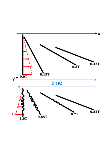
Figure 1: Sketch of numerical experiment: Initially the filament is straight. It rotates and translates while advected by ${\bm{U}}=\dot{\gamma}y\hat{\rm x}$ with $\dot{\gamma}=S\sin(\omega t)$ over the first-half of the cycle. In the second half the filament rotates and translates back but in addition buckles if its elastoviscous number is large enough. The flow ${\bm{U}}$ at $t=T/4$ (top panel) and $t=3T/4$ (bottom panel) are shown as red arrows.

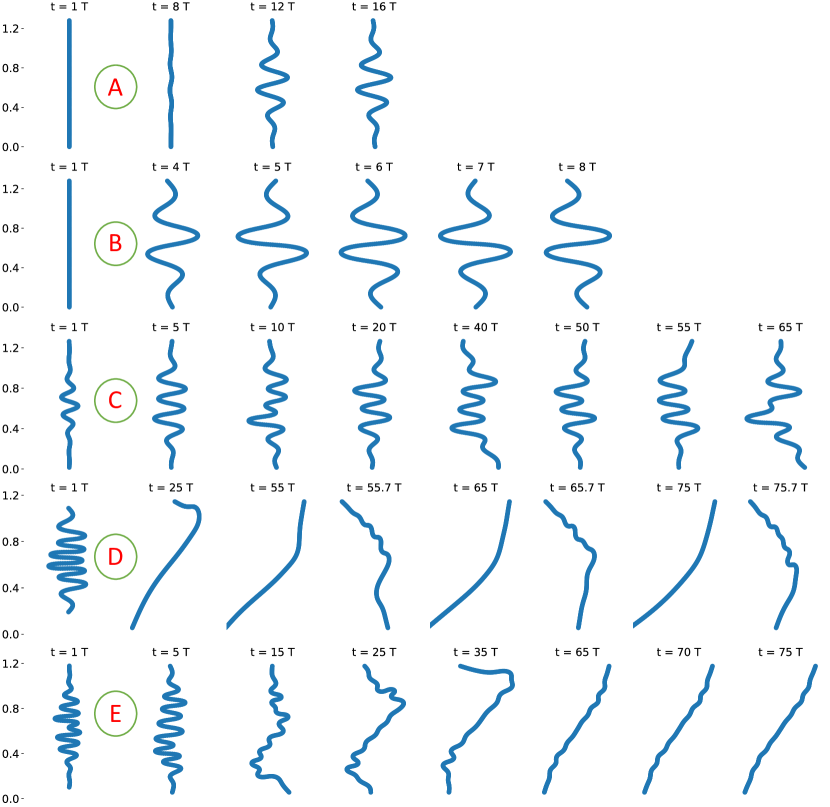
Figure 2: Kaleidoscope of dynamical behavior: (A) Periodic buckling ($\overline{\mu}=1.46\times 10^{6}$, $\sigma=1.5$): The filament is buckled after $8$ cycles and repeats itself after every cycle afterwards. Till cycle $8$ the filament is not straight but slightly deformed from its initial straight shape. This small deformation is barely noticeable in this figure. (B) Two-period ($\overline{\mu}=0.67\times 10^{6}$, $\sigma=0.75$): The shape of the filament is either of two shapes, which are mirror images of each other, at odd and even cycles. (C) and (D) The two types of Complex phases: (C)For $\overline{\mu}=3.35\times 10^{6}$, $\sigma=1.5$: The filament never repeats itself. (D) For $\overline{\mu}=6.7\times 10^{6}$, $\sigma=0.75$: The filament shows spatiotemporally complex behavior but for late cycles, the filament (almost) repeats at the end of every cycle ($nT$) ($t=55T,65T,75T$) but not at any other time. To illustrate, we show the snapshots at $t=55.7T,65.7T,75.7T$ – the shape of the filament is different from one another. Note, the filament shows maximum buckling, not at the end of a cycle, but at times in-between the cycles, i.e., at $t=(n+p)T$, where $n$ is an integer and $0<p<1$. (E) Complex transients($\overline{\mu}=16.75\times 10^{6}$, $\sigma=1.5$): Filament shows complex behavior for early periods but repeats itself at late times.

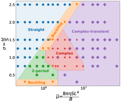
Figure 3: Phase diagram from time-dependent numerical simulations in the $\overline{\mu}$–$\sigma$ parameter space; $\left(\sigma=\frac{\omega}{S},\overline{\mu}=\frac{8\pi\eta SL^{4}}{B}\right)$. Here $\omega$ is rate of change of strain, $S$ is strain rate, $\eta$ is the viscosity, $L$ is length of the filament, and $B$ is the bending modulus. Initially, the filament is freely suspended in the shear flow, see Figure. 1. We show five different dynamical phases in the system represented by five symbols. Straight ($\bullet$) : The filament comes back to the initial position in the straight configuration after every period. Periodic buckling ($\blacktriangledown$):- The filament comes back in the buckled configuration after every period. Two-period ($\blacksquare$) : The filament repeats its configuration not after every but after two-period. Complex($\bigstar$): The filament buckles into complex shape with very high mode of buckling instability. Complex–transients($\blacklozenge$) : Filament shows long transients with complex shape but at late times, the shape of the filament repeats itself. The boundary between the complex and complex-transient phase is difficult to clearly demarcate.

Initially, the filament is placed along the $y$ direction with its head at $y=0$, see Figure. 1. We use $N=256$, $K=16$ and $a=d$ in all our simulations and vary both $\sigma$ and $\overline{\mu}$ to explore a variety of dynamical behaviour.

As we impose an external linear flow with a period $T$, it is useful to look at stroboscopic snapshots of the filament separated by time $T$. We note that in some cases filament does not return to its original position at the end of a cycle. When that happens time-reversal invariance is already broken even if the shape of the filament remains unchanged. We call this swimming. In this paper we focus not on swimming but on how the shape of the filament changes.

III.1 Dynamical phases

Based on the shape, a kaleidoscope of qualitative behavior emerges that we classify into five different dynamical phases. For small elastoviscous number ($\overline{\mu}$) the filament comes back to its original position undeformed at the end of every period (not shown in Fig. 2). As $\overline{\mu}$ is increased, the filament is buckled at the end of every period; see Fig. 2 panel A. On increasing $\overline{\mu}$ further we reach a phase where two buckled states, which are mirror images of each other, alternate at the end of even and odd periods – a period–two solution; see Fig. 2 panel B. At even higher $\overline{\mu}$ the shape of the filament at the end of every cycle is different – the filament never repeats itself. We continue these simulations to long times. In some cases the shape of the filament never repeats itslf, see Figure. 2 panel C. In some other cases, the shape of the filament is almost repeated at the end of every period, but the shape is different at all other times, e.g., consider the snapshots in Figure. 2 panel D. The shape of the filament at $65T$ and $75T$ are almost the same. But the shapes at $65.7T$ and $75.7T$ are not. We do not make a distinction between these two dynamical behavior – we call both of them complex. Finally, for large $\overline{\mu}$ we find that the shape of the filament shows complex spatiotemporal behaviour till intermediate times $t<60T$ but almost settles (it comes very close but does not repeat itself) to a fixed spatially complex shape at late times; see Fig. 2 panel E. By surveying a range of values for $\overline{\mu}$ and $\sigma$ we construct a phase diagram in Fig. 3. We find that the straight phase can go unstable in two ways, depending on the value of $\sigma$. It can either undergo a bifurcation to a two-period solution or go to a buckled phase which repeats itself. The buckled solution appears at end of every period, it is a time-reversible solution, the two-period solution is not. The boundary between the phases can be clearly demarcated except the boundary between the complex and the complex-transient phase. Thus it may be possible that there is a fractal boundary between these two phases. Fractal boundaries are not an uncommon occurance in many dynamical systems including transition to turbulence in pipe flows Schneider et al. (2007), different forms of spiral-wave dynamics in mathematical models of cardiac tissues Shajahan et al. (2007), and onset of dynamo in shell-models Sahoo et al. (2010). We have not explored this aspect in any detail in this paper. Except the region of the phase diagram where we find straight solutions, swimming solutions appear everywhere else.

III.1.1 Complex Phase

Let us first discuss in detail a representative simulation in the complex phase. As we focus on the shape of the filament we describe the filament in its intrinsic coordinates – its curvature ($\kappa$) as a function of material coordinate ($s$). We calculate curvature using a discrete approximation, see appendix A. In Fig. 4 we plot $\kappa$ versus $s$ for early times, at $t=T,10T,19T$ and $28T$, in Fig. 4(A) and for late times in Fig. 4(C), at t=$35T,45T,55T$ and $75T$. At all times, the curvature is zero at the two end of the filament, as dictated by the boundary conditions, and changes sign several times, i.e., a quite complex morphology is observed, as we show in Fig. 4(B) and Fig. 4(D) respectively. The minimum value of the radius of curvature is approximately $10d$ where $d$ is the diameter of each bead or alternatively the thickness of the filament. A sine transform of the $\kappa(s)$ to $\hat{\kappa}(q)$ shows several peaks, For $q\gtrapprox 20$ the $\hat{\kappa}$ is practically zero, see Appendix C. This demonstrates that our simulations are well resolved to capture the phenomena we observe. As the filament moves in the fluid it changes the background flow. In Fig. 4(E) and Fig. 4(F) we plot a typical phase-potrait of the velocity of the flow (after subtracting out the background velocity) at a fixed Eulerian point. For small $\overline{\mu}$, in the part of the phase diagram where the filament always remain straight, the phase potrait is a simple closed curve as shown in orange in Fig. 4(E) and Fig. 4(F). For the case where the filament is in the complex phase we obtain a non-trivial attractor.

There is another intriguing feature seen in some of the runs in the complex phase: although the filament never repeat itself exactly in the $\kappa$–$s$ space it comes very close to periodic behavior with a large period, in one case $30T$.

III.1.2 Complex–Transient phase

Next we turn to the phase we call Complex–Transient. Here the behavior is the same as the Complex phase upto quite late times, e.g., $60T$ after which the filament comes to almost the same shape at the end of every period. Here also the dynamics of the filament is not strictly periodic. The shapes, which are complex, change but very slowly over time. This slow drift in the configuration space can be measured by calculating

$$K(p-m)=\left[\int\mid\kappa(s,pT)-\kappa(s,mT)\mid^{2}ds\right]^{1/2}$$ (5)

where $m>60$ is a period where the filament has already reached its late time behavior. We find $K(p-m)\sim(p-m)$, for not too large values of $p-m$. i.e., an algebraic growth. We perform another numerical experiment. We take the filament in its late almost stationary configuration and add a small perturbation and then evolve again. The perturbation goes to zero very quickly, the filament goes back to its almost stationary configuration.

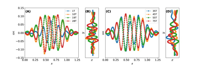
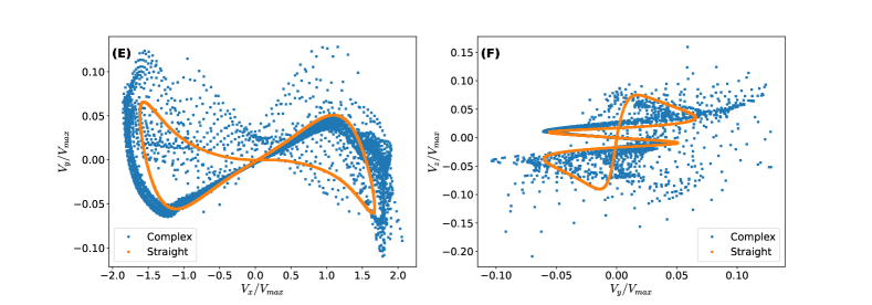
Figure 4: Evolution in the complex phase: ($\overline{\mu}=3.35\times 10^{6}$, $\sigma=1.5$) The filament shows complex behavior and does not repeat in real space or configuration space ($t<45T$) 9. (A) Curvature ($\kappa$) as a function of material coordinate, $s$, of the filament at early cycles, $t=T,10T,19T$ and $28T$. (B) Image of the filament at the same times. (C) and (D) Same as (A) and (B) but for late times. (E,F) Phase portrait of tracer velocity at a fixed Eulerian point for late cycles $t=45T$–$75T$.

III.2 Stroboscopic map

So far we have studied the different dynamical phases through time-stepping our numerical code. Potentially, both the complex and complex-transient phase are spatiotemporally chaotic. But a time-stepping code however accurate accumulates error which grows with the number of time-steps taken. To investigate the fate of the filament at late times we do have to integrate over long times. Hence we need additional evidence to confirm the existence of chaos in this problem.

We start by defining the stroboscopic map, $\mathcal{F}$,

$$\kappa(s,T)=\mathcal{F}\kappa(s,0)$$ (6)

The dynamical system obeyed by the filament, equation (1a), is non-autonomous because the external flow ${\bm{U}}$ is an explicit function of time, the map $\mathcal{F}$, which is generated by integrating (1a) over exactly one time period $T$, is autonomous. This is a map of $N$-dimensional space onto itself where $N$ is the number of beads. The function $\kappa(s,t)$ at $t=nT$ and $t=(n+1)T$ are related by one iteration of this map. We proceed to study the fixed points and periodic orbits of this map as a function of the parameters, $\overline{\mu}$ and $\sigma$, following Refs. Auerbach et al. (1987); Cvitanovic et al. (2005). Such techniques have been used widely to study transition to turbulence in high-dimensional flows Kerswell (2005); Suri et al. (2020); Page et al. (2020) and has also been applied to other fields of fluid dynamics Franco-Gómez et al. (2018); Gaillard et al. (2021). The detailed numerical techniques are described in appendix A.

In Fig. 5 we show several examples of the solutions we obtain, for a fixed $\sigma=0.75$ as a function of $\overline{\mu}$. For small $\overline{\mu}=0.17\times 10^{6}$ we obtain only one fixed point and it corresponds to $\kappa(s)=0$, i.e., a straight filament. At $\overline{\mu}=0.33\times 10^{6}$ in addition to the straight filament a new fixed point appears, where $\kappa$ is zero at one end, changes sign once roughly at the middle of the filament and has two maximas. We show the shape of the filament in Fig. 5(B1). At exactly this point in the phase diagram, see top line in Fig. 5, obtained from the evolution code, we find a straight filament. This implies, either of the two possibilities: one, the new solution is unstable; two both the solutions are stable but the evolution code lands up in the straight one because of the initial condition we chose. Next at $\overline{\mu}=0.33\times 10^{6}$ we no longer find any fixed points. We find two periodic orbits, one that is a two–period Fig. 5(C1) and one with four periods Fig. 5(C2). The two solutions in the two-period solution are mirror images of each other. At the same place in the phase diagram the evolution code finds the same two–period solution. Increasing $\overline{\mu}$ to $0.84\times 10^{6}$ we find that the four-period solution has disappeared, two two–period solutions exist, Fig. 5(D). At even higher values of $\overline{\mu}$ we start to obtain many solutions. We show a few examples in Fig. 5(F), Fig. 5(G), and Fig. 5(H). This is the region of phase space where complex and complex-transient dynamical phases are seen.

To summarize, by turning our system of coupled non-autonomous differential equations, (1a) to an autonomous stroboscopic map and by studying the solutions of the map we find further support of breakdown of time reversibiity and appearence of chaos that we had already seen from the evolution of the differential equations. We demonstrate that the first appearence of breakdown of time-reversibility is through a period-two bifurcation. The map has many solutions and the number of solutions increases as we increase $\overline{\mu}$.

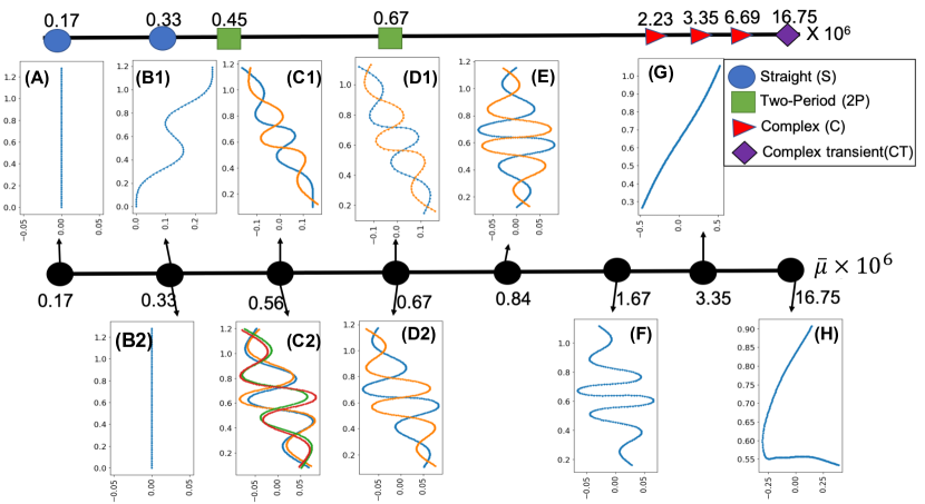
Figure 5: Solutions of stroboscopic map in real space for $\sigma=0.75$ for different values of $\overline{\mu}$. We find multiple co-existing solutions as we increase $\overline{\mu}$ (black symbols from left to right) indicating the complexity of the system. We compare this solutions with the solutions obtained at late times from the evolution code at the same points in the phase diagram.

III.3 Mixing of passive tracer

Next we study how passive tracers are transported by the flow generated by the presence of the filament for parameters in the complex phase. The velocity of the flow, ${\bm{U}}(\bm{r})$, at any Eulerian point, $\bm{r}=(x,y,z)$ is given in (4a). The equation of motion of a passive tracer, whose position at time $t$ is given by ${\bm{X}}(t)$, is

$$\frac{d{\bm{X}}}{dt}={\bm{U}}(\bm{r})\delta(\bm{r}-{\bm{X}})\/.$$ (7)

We solve (7) simultaniously with (4a) and for $N_{\rm p}$ tracers. The tracers are introduced into the flow on concentric circles in the $x$–$y$ plane, Fig. 6(A), after approximately $10$ cycles, when the flow has reached a statistically stationary They are colored by radius of the circle on which they lie on at the initial time. After $8$ periods, $t=8T$, we find that the outer rings are still somewhat intact but the inner rings have somewhat merged with each other and also moved out of the $x$–$y$ plane. At even later time, $t=256T$, we find the tracer particles are well mixed with each other.

In the rest of this section, we set $t=0$ at the time the tracers are introduced. To obtain a quantitative measure of mixing we define

$$\Delta{\bm{X}}^{\rm k}_{\rm j}\equiv{\bm{X}}^{\rm k}((j+1)T)-{\bm{X}}^{\rm k}(jT)\quad\/,$$ (8)

the net displacement of the ${\rm k}$-th tracer particle over the $j$-th cycle – $t=jT$ to $t=(j+1)T$, where $j$ is an integer. The net displacement of the ${\rm k}$-th tracer after $q$ cycles is

$$\bm{\rho}^{{\rm k}}(q)=\sum_{j=1}^{q}\Delta{\bm{X}}^{{\rm k}}_{{\rm j}}\/.$$ (9)

The total mean square displacement, averaged over all the tracers, at the end of $q$ cycles is given by

$$\left\langle\rho^{2}(q)\right\rangle\equiv\frac{1}{N_{\rm p}}\sum_{{\rm k}=1}^{N_{\rm p}}\lvert\bm{\rho}^{{\rm k}}(q)\rvert^{2}$$ (10)

If the tracers diffuse then we expect $\left\langle\rho^{2}(q)\right\rangle\sim q$ for large $q$ Taylor (1922). In Fig. 6(D) we plot $\left\langle\rho^{2}(q)\right\rangle$ versus $q$ in log-log scale. Clearly $\left\langle\rho^{2}(q)\right\rangle$ increases faster than $q$ but slower than $q^{2}$! Could it be possible that the tracers show Levy-like superdiffusion ?

If this is true then the probability distribution function (PDF), $\mathcal{P}$, of the displacement $\Delta X^{{\rm k}}_{{\rm j}}$ must have a power-law tail with an exponent $\gamma\geq-2$. We probe this by calculating the cumulative probability distribution (CDF) function for $\Delta X^{{\rm k}}_{{\rm j}}$ for all $j$ and $k$. We calculate the CDF using rank-order method. The advantace of using the CDF is that unlike the PDF it is not plagued by binning error. The CDF of $\Delta X^{{\rm k}}_{{\rm j}}$ is different for each of its components. The CDF of the out-of-plane component, $X_{3}$, has an exponential tail. The CDF of the two in-plane components are qualitatively similar, hence we calculate $\Delta s=\sqrt{X_{1}^{2}+X_{2}^{2}}$ and plot its CDF, $\mathcal{Q}(\Delta s)$, calculated by the rank-order method, in Fig. 6(E). The tail of the CDF has a slope approximately equal to $-3$, which implies that the tail of the corresponding PDF has a slope of approximately $-4$. Thus, by the central limit theorem we conclude that the tracers to show diffusion, not superdiffusion. However, as the PDF has power-law tail we expect that very long averaging over very many number of tracer particles is necessary for convergence. This explains why we do not observe clear evidence of diffusion from the mean square displacement.

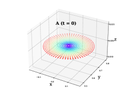
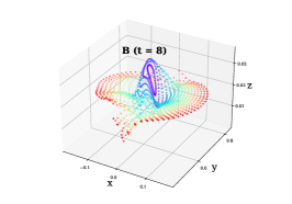
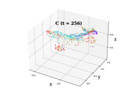
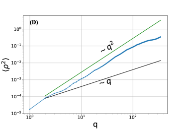
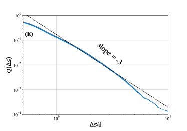
Figure 6: Mixing of passive tracer: (A) to (C) Positions of tracer particles at different times for the filament in complex phase ($\overline{\mu}=3.3\times 10^{6}$, $\sigma=1.5$). Initially, the tracers are placed on concentric circles, color coded by their distance from the center of the circles. The mixing of the colors show the mixing of the scalars. (D) Mean squre displacment (MSD), $\left\langle\rho^{2}\right\rangle(qT)$, defined in (10), as a function of $q$ in log-log scale. We also plot two lines with slopes $1$ and $2$. (E) Cumulative probability distribution function, $1-\mathcal{Q}(\Delta s)$ as a function of $\Delta s=\sqrt{X_{1}^{2}+X_{2}^{2}}$ ($X_{1}$ and $X_{2}$ are in-plane coordinate of the tracers).

IV Conclusion

To summarize, we numerically study the motion of a freely-floating elastic filament in a linear shear flows that changes periodically with time, at zero Reynolds number. We find that elastic nonlinearies of the filament are responsible for breakdown of time-reversal symmetry. The first signature of this breakdown, which appears as we increase the elasto-viscous number, is that the filament starts to swim – it does not return to its initial poistion after one period, although it returns to the same shape. As the elastoviscous number is increased we find period-two bifurcation and eventually what could be spatiotemporally chaotic behavior of the shape of the filament. Surprisingly, at quite large elastoviscous number we find that chaos is suppressed at late times – the filament returns to the same shape at the end of every period but does not repeat itself between the periods. We also demonstrate that such a filament is an efficient mixer of a passive scalar. Few comments are now in order.

Our numerical experiments corresponds, roughly, to the same range of elastoviscous parameters as the recent experiments Liu et al. (2018) of flexible filaments in constant-in-time shear flow and our code reproduces the behaviour seen in these experiments. Hence we expect it will be possible to experimentally confirm our results, at least qualitatively. Intriguingly, the spatiotemporally chaotic behavior is observed within a window of values of the elastoviscous number for a fixed value of $\sigma$.

We have not confined the numerical solution of our problem to two dimensions. The filament could, in principle, bend out-of-plane when buckled, but it never does. We expect, if torsion is included the filament will bend out of the plane and also break the reflection symmetry. However, the passive tracers driven by the filament do move out of the plane.

In addition to elastic nonlinearity, we have included non-local viscous interaction. In its simplest approximation a filament in a viscous flow can be described by including only the diagonal term (${\rm i}={\rm j}$) in the Rotne–Prager tensor Goldstein et al. (1998) in (1b). We have checked that for such a model we also find spatiotemporally chaotic behavior, which will be reported elsewhere.

Spatiotemporally chaotic systems are rare in nonlinear systems in one space dimension, e.g., the one-dimensional Burgers equation does not show chaotic behavior. When described in terms of its intrinsic coordinates our filament could, naively, considered to be, a spatiotemporally chaotic one dimensional system. However, this is not true because the external shear cannot be captured only with the intrinsic coordinates.

A single rigid ellipsoid in a shear flow shows low-dimensional chaotic motion for appropriate choice of parameters Radhakrishnan et al. (1999); Lundell (2011); Nilsen and Andersson (2013). Hence, from a fundamental point of view, it is not a surprise that a deformable thread in a time-dependent shear can show spatiotemporally chaotic behaviour. However, it has never been demonstrated before.

For a small enough filament, e.g., a single large polymer molecule, thermal effects that we have ignored, may be important. We have ignored them for two reasons. First, in many experimental situations Liu et al. (2018) the filament is large enough that the thermal fluctuations may not be crucial. Second, we want to address the fundamental question of emergence of chaotic behavior due to elastic nonlinearities in the absence of any external stochastic fluctuations. We further emphasize that most strategies of increasing mixing in microfluidics rely on having a non-zero but small molecular diffusivity – “ For efficient mixing to be achieved, the velocity field must stir together different portions of the fluid to within a scale that is small enough for diffusion to take over and homogenize the concentrations of the advected quantities.” Aref et al. (2017). By contrast, we operate at zero molecular diffusivity – our system is diffusive even at infinite Peclet number.

Appendix A Model and Method

A.1 Model

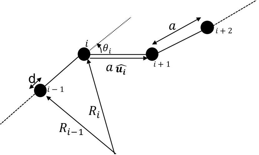
Figure 7: Schematic of a freely jointed bead-rod chain. We show $a>d$ for illustration, but we use $a=d$ for our simulation.

We use the bead-spring model for the numerical simulation of the filament in a flow Larson et al. (1999); Guglielmini et al. (2012); Nazockdast et al. (2017); Slowicka et al. (2019); Wada and Netz (2006); Żuk et al. (2021). The model consists of $N$ spherical beads of diameter $d$, connected by overdamped springs of equilibrium length $a$, see Fig. 7. The total length of the filament is $L$. The position of the center of the $i$-th bead is $\bm{R}_{\rm i}$, where $i=1,\ldots N$. The equation of motion for the $i$-th bead is given by Wada and Netz (2006):

$$\partial_{t}R_{\rm i}^{\alpha}=-\sum_{j=0}^{N-1}M_{\rm ij}^{\alpha\beta}(\bm{R}_{\rm ij})\frac{\partial\mathcal{H}}{\partial R_{\rm j}^{\beta}}+U^{\alpha}_{0}(\bm{R}_{\rm i})\quad\/.$$ (11)

Where $\bm{R}_{\rm ij}=\bm{R}_{\rm j}-\bm{R}_{\rm i}$, $\mathcal{H}$ is the elastic hamiltonian, $\partial(\cdot)/\partial(\cdot)$ denotes the partial derivative, the greek indices run from $1$ to $D$, where $D=3$ is dimensionality of space. Repeated greek indices are summed. The velocity of the background flow, ${\bm{U}}_{0}$ is given by

$${\bm{U}}_{0}(x,y)=\dot{\gamma}y\hat{\rm x}\/,\quad\text{with}\quad\dot{\gamma}=S\sin(\omega t)\/,$$ (12)

being the time–periodic strain—rate and $\omega\equiv 2\pi/T$.

The hydrodynamic interaction between the beads is encoded by the Rotne–Prager mobility tensor $M_{\rm ij}(\bm{R})$ Rotne and Prager (1969); Guazzelli and Morris (2011); Brady and Bossis (1988); Kim and Karrila (2013):

$$M_{\rm ij}^{\alpha\beta}(\bm{R})=\left\{\begin{array}[]{ll}\frac{1}{8\pi\eta R}\left[\delta^{\alpha\beta}+\frac{R^{\alpha}R^{\beta}}{R^{2}}+\frac{d^{2}}{2R^{2}}\left(\frac{{\delta^{\alpha\beta}}}{3}-\frac{R^{\alpha}R^{\beta}}{R^{2}}\right)\right]&,{\rm i}\neq{\rm j}\\ \frac{1}{3\pi\eta d}\delta^{\alpha\beta}&,{\rm i}={\rm j}\end{array}\right\}.$$ (13)

Here $\eta$ is viscosity of the fluid, and $R=\left|\bm{R}\right|$.

The Hamiltonian of the system, $\mathcal{H}$, is $\mathcal{H}=\mathcal{H}_{\rm B}+\mathcal{H}_{\rm S}$ – we do not consider torsion. Here $\mathcal{H}_{\rm B}$ and $\mathcal{H}_{\rm S}$ are contributions from bending Montesi et al. (2005); Bergou et al. (2010) and stretching Wada and Netz (2006, 2007) respectively. The bending energy of a filament is given by Powers (2010):

$$\mathcal{H}_{\rm B}=\frac{B}{2}\int\kappa^{2}(s)ds,$$ (14)

where $B$ is the bending modulus, $\kappa$ is curvature, and $s$ is the material coordinate. The discrete form of $\mathcal{H}_{\rm B}$ is Bergou et al. (2008, 2010); Montesi et al. (2005):

$$\mathcal{H}_{\rm B}=aB\sum_{i=0}^{N-1}\kappa_{i}^{2}=\frac{B}{a}\sum_{i=0}^{N-1}\hat{\bm{u}}_{i}\cdot\hat{\bm{u}}_{i-1}=\frac{B}{a}\sum_{i=0}^{N-1}\cos\theta_{i}\/,$$ (15)

where

$$\kappa_{\rm i}=\frac{2}{a}\tan\left(\frac{\theta_{\rm i}}{2}\right)\approx\frac{\sin\left(\theta_{\rm i}\right)}{a}=\frac{\left|\hat{\bm{u}}_{\rm i}\times\hat{\bm{u}}_{{\rm i}-1}\right|}{a},$$ (16a)

$$\hat{\bm{u}}_{\rm i}=\frac{\bm{R}_{{\rm i}+1}-\bm{R}_{\rm i}}{\lvert{\bm{R}_{{\rm i}+1}-\bm{R}_{\rm i}}\rvert}\quad\/,$$ (16b)

and $\theta_{\rm i}$ is the angle between two consecutive unit vectors $\hat{\bm{u}}_{\rm i}$ and $\hat{\bm{u}}_{\rm{i-1}}$ (see Fig. 1(A)). In the second step of (15), we have dropped a constant term. In the last step of (16a), we have used the small-angle approximation Montesi et al. (2005).

The stretching energy is discretized Wada and Netz (2006, 2007) as:

$$\mathcal{H}_{\rm S}=\frac{H}{2a}\sum_{{\rm i}=0}^{N-1}(\lvert{\bm{R}_{{\rm i}+1}-\bm{R}_{\rm i}}\rvert-a)^{2}\/,$$ (17)

where $H$ is the stretching modulus. We ignore thermal fluctuations.

A.2 Non–dimensionalization

We use $L$ and $1/S$ as our characteristic scales for length and time, respectively. The evolution equation in non-dimensional form is:.

$$\partial_{\tilde{t}}\widetilde{R}_{\rm i}^{\alpha}=-\frac{1}{\overline{\mu}}\sum_{j=0}^{N-1}\widetilde{M}_{\rm ij}^{\alpha\beta}(\widetilde{R}_{\rm ij})\left[\frac{\partial\widetilde{\mathcal{H}}_{\rm B}}{\partial\widetilde{R}_{\rm j}^{\beta}}+K\left(\frac{L}{d}\right)^{3}\left(\frac{d}{a}\right)\frac{\partial\widetilde{\mathcal{H}}_{\rm S}}{\partial\widetilde{R}_{\rm j}^{\beta}}\right]\\ +\tilde{y}\sin{\sigma\tilde{t}}\quad\/.$$ (18)

Here $\tilde{(\cdot)}$ denotes non-dimensional quantities. We get the following dimensionless parameters: The elasto-viscous number,

$$\overline{\mu}\equiv\frac{8\pi\eta SL^{4}}{B},$$ (19)

the non-dimensional frequency,

$$\sigma\equiv\frac{\omega}{S},$$ (20)

and the ratio of stretching to bending,

$$K\equiv\frac{Hd^{2}}{B}.$$ (21)

All the parameter values are shown in table 1.

Appendix B Numerical Implementation

We use the adaptive Runge-Kutta method Press et al. (2007) with cash-karp parameters Press and Teukolsky (1992); Cash and Karp (1990) to evolve the system. We use time-step, $\Delta t$, such that

$$\tilde{\Delta}=\frac{B\Delta t}{8\pi\eta L^{4}}=10^{-11}\text{ -- }10^{-12}$$ (22)

We use numerical accuracy of order $10^{-6}$ Press et al. (2007); Press and Teukolsky (1992); Cash and Karp (1990). We use CUDA to parallelize the code .

The dimensionless frequency, $\sigma$, must be small enough such that the Stokesian approximation remains valid. We use $K=16$ (see table 1) for all the simulations. Note that (15) is exact for an inextensible filament. In our case, the total length of the filament changes at most by $2\%$ – the filament is practically inextensible. Hence (15) remains a reasonable approximation. Our code reproduces the experimental results by Liu et. al. Liu et al. (2018) (see Fig. 8).

Parameters	Simulation values
Number of beads, $N$	$256$
Equilibrium distance between beads, $a$	$0.005$
Filament diameter, $d$	$0.005$
Filament length, $L$	$1.28$
Bending modulus, $B$	$2\times 10^{-5}\mbox{--}8\times 10^{-3}$
Strain Rate amplitude, $S$	$2$
Viscosity, $\eta$	$10$
Rate of change of strain rate, $\omega$	$1\mbox{--}6$
Time-step, $\Delta$	$10^{-4}\mbox{--}10^{-6}$
Elasto-viscous number, $\overline{\mu}=\frac{8\pi\eta SL^{4}}{B}$	$1.7\times 10^{5}\mbox{--}6.8\times 10^{7}$
Frequency parameter, $\sigma=\frac{\omega}{S}$	$0.5\mbox{--}3$
Stretching-bending modulus ratio, $K=\frac{Ha^{2}}{B}$	$16$

Table 1: Parameters of simulation. Earlier studies have used $N=20-40$ Wada and Netz (2006), $N=40$ Slowicka et al. (2019), N=400 Chakrabarti et al. (2020)

Figure 8: Comparison with experimental results: We reproduce the experimental results of Ref. Liu et al. (2018). The filament lies along the x-axis. It is advected by a flow ${\bm{U}}=(\dot{\gamma}y,0)$, where $\dot{\gamma}$ is the shear rate. The flow is constant in time. We observe different dynamical behavior for different $\overline{\mu}$. The grey background are figures from Ref. Liu et al. (2018), and the white background are results of our simulation. Initially, we add small perturbation to the filament but ignore thermal fluctuations. The $\overline{\mu}_{\rm E}$ and $\overline{\mu}_{\rm S}$ are the values of $\overline{\mu}$ from experiments and our simulations respectively.

Appendix C Detailed description of the dynamical phases

Our simulations reveal five different dynamical phases which we call – straight, buckling, two-period, complex and complex–transients (see Fig. 3 from main text).

For each case, we describe the dynamics through the morphology of the filament. This we do in two ways:

1. Extrinsic (real space) – actual shape of the filament.

2. Intrinsic (configurational space) – curvature ($\kappa$) of the filament as a function of the material coordinate($s$). Our classification of dynamical phase is based on the intrinsic coordinates. Conversion between extrinsic to intrinsic coordinates is done using (16) – this conversion is unique. Although the inverse is not true. To impose uniqueness, we fix the position of the first bead and slope of the bond to the next one.

C.1 Straight (S)

The filament does not buckle but remains straight all through its evolution, the curvature remains zero always.

C.2 Periodic buckling (B)

The filament develops buckling instability. The filament settles into periodic behavior after initial transients and repeats itself stroboscopically (after every cycle) both extrinsically and intrinsically.

C.3 Two-period (2P)

The filament does not repeat itself after every period but after every two periods. Also, the filament does not come back to its position but is rotated after two-cycles – which we call swimming.

C.4 Complex (C)

The filament rotates in the first half of the cycle (see Fig. 1). In the second half, it buckles. In Fig. 9 (A), we plot the filament at the end of $1$st, $10$th, $19$th and $28$th cycle for $\overline{\mu}=3.35\times 10^{6}$, $\sigma=1.5$) – the filament never repeats itself. In Fig. 9 (B), we plot the curvature ($\kappa$) of the filament as a function of arc-length ($s$) at the same times. This shows too that the shape of the filament never repeats at the end of each cycle. Even at late times $t>60T$, the filament does not repeat itself at the end of a cycle – see Fig. 9(C) where we plot the shape of the filament at $t=35T,45T,...,75T$. The corresponding plot of $\kappa$ versus $s$ is shown in Fig. 9(D). Here it may seem that the filament comes close to its previous shapes but a careful look tells us that it never completely repeats itself. Note that, the $\kappa$ – $s$ plot for $t=35T$ is very close to the one at $t=65T$, although not exactly the same. The same is true for $t=45T$ and $t=75T$. This suggests that there maybe a very high period solution to the stroboscopic map. A sine transform of the $\kappa(s)$ to $\hat{\kappa}(q)$ shows several peaks, For $q\gtrapprox 20$ the $\hat{\kappa}$ is practically zero (Fig. 10) This demonstrates that our simulations are well resolved to capture the phenomena we observe.

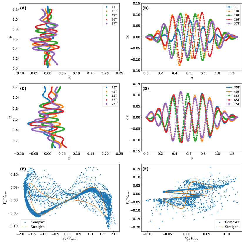
Figure 9: Evolution of the filament in complex phase ($\overline{\mu}=3.35\times 10^{6}$, $\sigma=1.5$) The filament shows complex behavior for cycles at intermediate times, (A) real space; (B) configurational space. (C,D) For late cycles also, the filament either does not repeat itself or comes close to repeating itself with very high time-period. The filament shows maximum compression at the end of cycle. (E,F) Phase portrait of tracer velocity late cycles $t=45T$–$75T$. For comparison we also show the phase potrait for a case in the straight phase (organge).

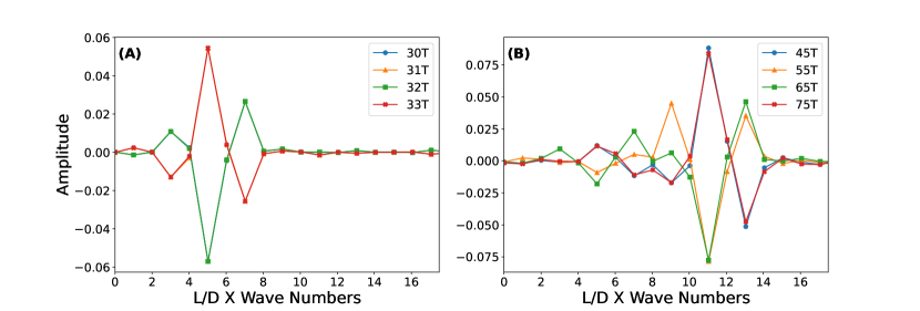
Figure 10: Discrete sine transform for two-period phase (A), and complex phase (B).

Note that, in some cases of this complex phase, at late times, the filament achieves the most buckled state (as measured by total elastic energy) not at the end of the cycle but somewhere in between. One such case is shown in Fig. 11 for $\overline{\mu}=6.7\times 10^{6}$ and $\sigma=0.75$. The $\kappa$–$s$ plot at the end of every cycle comes very close to repeating itself – Fig. 11(B). The corresponding plots of the filament in real space, is shown in Fig. 11(A), are also very close to one another although do not overlap everywhere. However, if we loook at intermediate times e.g. at $t=65.7T...75.7T$, we find that the filament does not repeat itself, Fig. 11(C,D).

To measure the disturbances in the flow due to moving filament, we calculate the time series of flow disturbance (${\bm{U}}-{\bm{U}}_{0}$) at an Eulerian point $\bm{r}=[0,L/2,2d]$. The numerical method is described in the main body of the paper, see also chapter 8 of Ref. Kim and Karrila (2013). The Eulerian point is chosen to be just above the $XY$ plane such that the filament does not overlap with it. We show the phase portraits of fluctuating velocity at late times ($t=40T$ to $t=75T$) in Fig. 9, Fig. 11(E,F) respectively. Note that, the velocity values are larger compared to the straight phase (Fig. 9(E,F)).

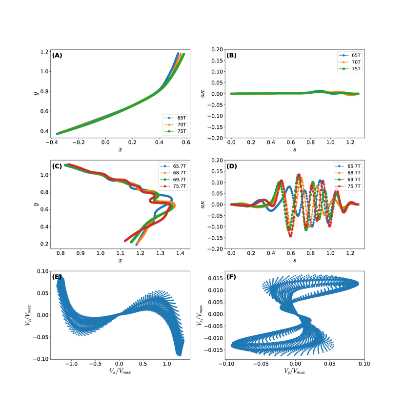
Figure 11: Evolution of the filament in the complex phase ($\overline{\mu}=6.7\times 10^{6}$, $\sigma=0.75$) The filament shows complex behavior at early cycles respectively in real space and configuration space. However, for late times ($t=65T,70T,75T$), the filament almost repeats itself at $nT$, where $n$ is an integer (A,B). Also note that, highest bending energy of the filament is at $(n+p)T$, $p\neq 0$ instead of $nT$ (C,D). The filament is shown stroboscopically for $p=0.7$ respectively in real space and configuration space. We observe that the filament does not repeat itself. (E,F) Phase portrait in $(x,y)$ and $(y,z)$ of Eulerian velocity at one point.

C.5 Complex transients:

The filament shows high mode of buckling. We compare the filament extrinsically and intrinsically at the end of $24$th, $34$th, $44$th cycle for $\overline{\mu}=3.35\times 10^{7},\sigma=1.5$ respectively in Fig. 12(A,B). The filament shows complex behavior and does not repeat itself for early periods ($t<60T$), similar to the complex phase. However, the complex behavior is transient and the filament comes very close to itself for late periods – at the end of a cycle ($t=80T,90T,100T$, see Fig. 12(C)) and intermediate times between cycle where the filament shows maximum buckling ($t=80.8T,90.8T,100.8T$, see Fig. 12(E)). The corresponding plots of $\kappa$–$s$ are shown in Fig. 12 (D)(F) – this also shows the almost–periodic behavior of filament at late times. In Fig. 12(G), we show the shapes at $t=80T,130T,180T$ and $230T$. Over such a long time scale, the shape does change. The corresponding $s$–$\kappa$ plots are shown in Fig. 12(H) In Fig. 12(I) and (J) we show the phase portrait of Eulerian velocity at $\bm{r}=[0,L/2,2d]$ for late times ($t>80T$).

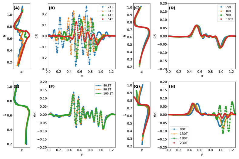
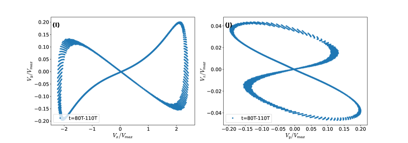
Figure 12: Evolution in the complex–transient phase: ($\overline{\mu}=3.35\times 10^{7}$, $\sigma=1.5$). The shape of the filament in (A)(C)(E) and the corresponding curvature is shown in (B)(D)(F). For early cycles (t $\leq$ 60T), the filament shows complex behavior and does not repeat itself (A,B), similar to the complex phase (see Fig. 9). For late cycles (t=70T …100T), although the filament does not repeat itself, it comes very close after every cycle (C,D,E,F). The filament shape, from the end of one cycle to next, changes very slowly, e.g. (E) shows the shape at $t=80.8T,90.8T,100.8T$. In (G), we show the shapes at $t=80T,130T\dots$. Over such a long time scale, the shape does change. (I)(J) Phase portrait of velocity at an Eulerian point for the late cycles.

Appendix D Stroboscopic map

We take a dynamical system approach to analyze the complex dynamics we observe. Such techniques have been used widely to study highly turbulent flows Kerswell (2005); Suri et al. (2020); Page et al. (2020) and has also been applied to other fields of fluid dynamics Franco-Gómez et al. (2018); Gaillard et al. (2021). Let us define an operator $\mathcal{F}$ such that:

$$\bm{\kappa}(T)=\mathcal{F}\bm{\kappa}(0)$$ (23a)

$$\mathcal{F}^{\rm p}=\mathcal{F}\mathcal{F}...\text{p times}...\mathcal{F},$$ (23b)

where $\bm{\kappa}=[\kappa_{1},\kappa_{2},\dots\kappa_{\rm i}\dots\kappa_{N}]$, where $\kappa_{\rm i}$ is the curvature at point ${\rm i}$. For a given $\bm{\kappa}$, the operator, $\mathcal{F}$, returns the values of $\bm{\kappa}$ after evolving the system for exactly one time-period. We look for fixed points and periodic orbits of this map Cvitanovic et al. (2005) by solving $\bm{\kappa}=\mathcal{F}^{\rm p}\bm{\kappa}$. The task is now to calculate the solutions of set of the non-linear equations:

$$\mathcal{N}_{\rm p}\bm{\kappa}\equiv\left(\mathcal{F}^{\rm p}-1\right)\bm{\kappa}=0$$ (24)

For example, $\bm{\kappa}=\bm{0}$, ${\rm p}=1$, is a solution for straight phase. The periodic buckling and two–period have non–zero curvature ($\bm{\kappa}$) solution respectively for ${\rm p}=1$ and ${\rm p}=2$. We use the Newton-Krylov method Knoll and Keyes (2004) based on Generalized Minimal Residual Method (GMRES) Saad and Schultz (1986) in jacobian–free way to find the solutions. It is described next.

D.1 Newton–Krylov

Figure 13: Flowchart for Newton–Krylov iteration. $\mathbb{K}$ is co-ordinate transformation from real to curvature space using equation (16). Similarly, $\mathbb{K}^{-1}$ is the inverse coordinate transformation from curvature to real space. We use the notation: $\mathcal{J}$ is jacobian of the operator $\mathcal{N}$, described in (24). We use $\rm{tol}=0.01$

The flow-chart of the algorithm is shown in Fig. 13. We start with a guess for the curvature, $\bm{\kappa}(0)$. Then we calculate the positions of the beads given by $\bm{y}\equiv[y_{1},...y_{2j-1},y_{2j},...y_{2N}]\equiv[R_{1}^{1},...,R_{j}^{1},R_{j}^{2},...R_{N}^{2}]$. We call this transformation $\bm{\kappa}$ to $\bm{y}$, $\mathbb{K}^{-1}$, such that:

$$\bm{y}(0)=\mathbb{K}^{-1}\bm{\kappa}(0)$$ (25)

Then we evolve in time from $t=0$ to $t={\rm p}T$ by solving (11) to obtain $\bm{y}({\rm p}T)$. Then we apply the inverse transformation, $\mathbb{K}$, to obtain

$$\bm{\kappa}({\rm p}T)=\mathbb{K}(\bm{y}({\rm p}T))$$ (26)

Then we check how accurately (24) is satisfied, i.e. we define

$$\text{error}=\frac{||\mathcal{N}_{\rm p}\bm{\kappa}||_{2}}{||\bm{\kappa}(0)||_{2}}.$$ (27)

The case for straight solution is dealt specially because in this case $\bm{\kappa}=0$. Here we use:

$$\text{error}=\frac{||\mathcal{N}_{\rm p}\bm{\kappa}||_{2}}{N*\text{tol}}$$ (28)

If the error is less than a preset tolerance, then we accept the guess ($\bm{\kappa}(0)$) as a solution, otherwise, we generate a new guess by

$$\bm{\kappa}(0)=\bm{\kappa}(0)+\delta\bm{\kappa},$$ (29a)

such that

$$\mathcal{J}\cdot\delta\bm{\kappa}=-\mathcal{N}_{\rm p}\bm{\kappa}(0).$$ (29b)

Here $\mathcal{J}$ is jacobian matrix of the operator $\mathcal{N}_{\rm p}$ computed at $\bm{\kappa}(0)$. We do not calculate $\mathcal{J}$, instead we calculate:

$$\mathcal{J}\cdot\delta\bm{\kappa}=\frac{\mathcal{N}_{\rm p}(\bm{\kappa}(0)+\varepsilon\delta\bm{\kappa})-\mathcal{N}_{\rm p}(\bm{\kappa}(0)-\varepsilon\delta\bm{\kappa})}{2\varepsilon}.$$ (30)

Here $\varepsilon$ is a step size Knoll and Keyes (2004). We use the GMRES Saad and Schultz (1986); Guennebaud et al. (2010) method in matrix-free way using (30) to find solutions of (29b). The operator $\mathcal{N}_{\rm p}$ is implemented as described in Figure. 13. The value of $\varepsilon$ should be small enough such that (30) is well approximated and large enough such that the floating point round–off errors are not too large Knoll and Keyes (2004). We compute $\varepsilon$ in the following way:

$$\varepsilon=\varepsilon_{\rm{rel}}\left(1+\frac{||\bm{\kappa}(0)||_{2}}{||\delta\bm{\kappa}(0)||_{2}}\right),$$ (31)

where $||\cdot||$ is the $2$nd norm, and $\varepsilon_{\rm{rel}}=10^{-4}$.

Note that, the conversion from curvature space to real space ($\mathbb{K}^{-1}$) is not unique. However, if we fix the position of the first bead and slope of the bond to the next one, it is unique. One advantage of using this method is that, it accounts for all the continuous symmetries (translation in $x$,$y$ direction) present in the system Cvitanovic et al. (2005).

Also note that the $\bm{\kappa}$ is the same for two filaments which has the same shape but are rotated with respect to each other. But the evolution of two such filaments are not the same, in principle, because the ambient flow depends on space. In some cases, we find the solutions such that the filament comes to the same shape as before but rotated. We call these solutions “swimming solutions”.