Quantum effects beyond mean-field treatment in quantum optics

Abstract

Mean-field treatment (MFT) is frequently applied to approximately predict the dynamics of quantum optics systems, to simplify the system Hamiltonian through neglecting certain modes that are driven strongly or couple weakly with other modes. While in practical quantum systems, the quantum correlations between different modes might lead to unanticipated quantum effects and lead to significantly distinct system dynamics. Here, we provide a general and systematic theoretical framework based on the perturbation theory in company with the MFT to capture these quantum effects. The form of nonlinear dissipation and parasitic Hamiltonian are predicted, which scales inversely with the nonlinear coupling rate. Furthermore, the indicator is also proposed as a measure of the accuracy of mean-field treatment. Our theory is applied to the example of quantum frequency conversion, in which mean-field treatment is commonly applied, to test its limitation under strong pump and large coupling strength. The analytical results show excellent agreement with the numerical simulations. Our work clearly reveals the attendant quantum effects under mean-field treatment and provides a more precise theoretical framework to describe quantum optics systems.

I Introduction

Mean-field treatment (MFT) is frequently applied to quantum many-body systems to reduce the degrees of freedom for readily solvable evolution equations. A typical application of MFT is demonstrated via the Ising model and achieves great success in predicting phase transitions (stanley1971mean, ). The main idea behind MFT is to focus on the average evolution of the systems by discarding the quantum correlation and fluctuation (kadanoff2009more, ), where the Bogoliubov inequality (bogolyubov2013method, ) serves as the mathematical foundation. Within the realm of quantum optics, MFT approximates the field of the optical modes to be complex numbers by neglecting quantum statistics and has been widely adopted. Such a treatment avoids the infinite dimension of number states and greatly simplifies the system dynamics to semi-classical nonlinear equations. It is demonstrated to be valid under weak coupling or strong drive. In a more general form, the MFT is also applicable to a subsystem by neglecting the quantum nature of part of the modes. The representative examples are the manipulation of atom states and squeezed light generation using strong coherent lasers, in which the strongly-pumped modes are isolated from the rest of the system and solved independently following the MFT.

Despite the great achievement in the application of MFT in quantum optics, its validity is challenged for significant quantum correlations and quantum fluctuations, which usually increase with the nonlinear interaction strength. Another circumstance is the urgent need for high-fidelity quantum information processors. The MFT on the control field limits the fidelity of quantum gates since the control field might entangle with the qubits. Even though these properties can be expressed fully by tracking the density matrix in a large Hilbert space, the computation complexity is beyond the capability of current computers and it is not always necessary when the system does not exhibit significant quantum features. Alternatively, it is efficient to reveal these omitted quantum effects neglected by MFT and add these elegant forms for a more accurate prediction of the system dynamics. When the quantum correlations of a subsystem are neglected, decoherence such as dephasing (blais2004cavity, ) of the remaining system could be expected by the reduced density matrix after tracing off the subsystem. Even worse, such correlation can affect the expectation values of the system and lead to the deviation from the prediction by MFT. Several studies have focused on the side effects of the coupling between a strong coherent field and a local quantum system, which is common in many quantum optics experimental platforms. It is expected that a high-intensity pump field can reduce the effect of dissipation (gea2002some, ; igeta2013fundamental, ; gea2010energy, ), while it may actually lead to the strong interaction between the signal and the pump modes (van2001classical, ). To suppress or make use of those correlation-induced phenomena beyond mean-field for high-fidelity quantum device implement, we should have a clearer understanding of how they depend on the experimental parameters thatoccurs with the rapid development of quantum nonlinear optics devices. A case in point is the advent of high-Q whispering gallery resonators (strekalov2016nonlinear, ), which enables the strong coupling strength among different modes to facilitate nontrivial quantum effects induced by correlation.

In this Letter, we offer the mean-field perturbation treatment (MFPT) to extract the incidental quantum effects for an open quantum system beyond the MFT. The general form of the incoherent dissipation and parasitic coherent interaction are derived when a quantum system is coupled to an MFT-applicable pump system. In addition, the indicators, as the measure of the accuracy of MFT are put forward to reveal the effect of quantum correlations on the system behavior. The theory is introduced with a complete analysis of the quantum frequency conversion process under a coherent pump, which agrees well with the simulation and shows how the property of the coherent pump affects the fidelity of the operation.

II Principle of Mean-Field Perturbation Treatment

For an open quantum system, the Lindblad master equation offers a general form to describe the system dynamics via (lindblad1976generators, ) $\dot{\rho}=\mathbb{L}\rho,$ where $\mathbb{L}$ is some generalized Liouville super-operator and can be written as

$$\mathbb{L}=-i[H,.]+\sum_{\alpha}\kappa_{\alpha}\mathscr{L}_{d_{\alpha}}[.],$$ (1)

where $H$ is the overall Hamiltonian for the system, $\mathscr{L}_{d_{\alpha}}[\rho]=2d_{\alpha}\rho d_{\alpha}^{\dagger}-d_{\alpha}^{\dagger}d_{\alpha}\rho-\rho d_{\alpha}^{\dagger}d_{\alpha}$ is the diagonalized Lindblad super-operator with the corresponding decoherence rate $\kappa_{\alpha}$ and the subscript $\alpha$ denotes different jump operator $d_{\alpha}$. In quantum optics systems, the $H$ is composed of the bosonic field operators of different optical modes, i.e. the annihilation operator $a$ and the creation operator $a^{\dagger}$. Those operators are spanned over an infinite-dimension Fock space, in which the equation is hardly solvable both analytically and numerically. Therefore, MFT is applied by simply replacing some of the bosonic operators with their expectation values in the simplified mean-field Hamiltonian $H_{\mathrm{MFT}}$. In general, for an $N$-th order term of the field operators in $H$ denoted as $\hat{N}=\widehat{N-M}\hat{M}$ with $M<N$, we can apply MFT by replacing the first term with its expectation value $\langle\widehat{N-M}\rangle_{0}(t)$ and obtain $\hat{N}_{\mathrm{MFT}}=\langle\widehat{N-M}\rangle_{0}(t)\hat{M},$ thus reducing the order from $N$ to $M$. Here, expectation values $\langle\widehat{N-M}\rangle_{0}(t)$ are solved according to their evolution under $H_{\mathrm{MFT}}$.

With the MFT, the system could be approximately solved with

$$\mathbb{L}_{\mathrm{MFT}}=-i[H_{\mathrm{MFT}},.]+\sum_{\alpha}\kappa_{\alpha}\mathscr{L}_{d_{\alpha}}[.].$$ (2)

As the generalized Liouville super-operators form an Abelian additive group, we can still consider the full model by including the influence of the dropped operators $\delta H=H-H_{\mathrm{MFT}}$ as

$$\delta\mathbb{L}=\mathbb{L}-\mathbb{L}_{\mathrm{MFT}}=-i[\delta H,.].$$ (3)

The essential idea of this work is to apply the perturbation of $\delta\mathbb{L}$ to the MFT, thus capturing the effects induced by the neglected quantum correlations. According to the general perturbation theory (yi2000perturbative, ), we obtain a set of equations to solve the evolution in power series of $\delta\mathbb{L}$ as

$$\frac{d}{dt}\rho_{i}=\mathbb{\mathbb{L}}_{\mathrm{MFT}}\rho_{i}+\delta\mathbb{L}\rho_{i-1},$$ (4)

with $i\geq 1$ denotes the order of the perturbation and $d\rho_{0}/dt=\mathbb{L}_{\mathrm{MFT}}\rho_{0}$ for the zeroth order. Eventually, the full solution of density matrix is $\rho=\sum_{i=0}^{\infty}\rho_{i}$ with the normalized condition $\mathrm{Tr}(\rho_{i})=0$ for $i\geq 1$.

To provide a concrete discussion about the proposed mean-field perturbation treatment (MFPT), we consider a general quantum system with a Hamiltonian of $H=H_{\mathrm{I}}+H_{0}^{\mathrm{A}}+H_{0}^{\mathrm{B}}$, which divided into two subsystems A and B, with the interaction between the subsystems as $H_{\mathrm{I}}=\sum_{j=1}^{m}F_{j}^{\mathrm{A}}F_{j}^{\mathrm{B}}$, which is decomposed into $m$ tensor products of operators in each subsystem as $F_{j}^{\alpha}$ ($\alpha\in\{\mathrm{A},\mathrm{B}\}$). We propose two approaches to apply the MFPT: (1) The symmetric MFPT that applies the MFT to the interaction Hamiltonian symmetrically to both subsystems as

$$H_{\mathrm{I},\mathrm{MFT}}=\sum_{j=1}^{m}\left(\langle F_{j}^{\mathrm{A}}\rangle_{0}F_{j}^{\mathrm{B}}+F_{j}^{\mathrm{A}}\langle F_{j}^{\mathrm{B}}\rangle_{0}\right)$$ (5)

with $\delta H=\sum_{j=1}^{m}\delta F_{j}^{\mathrm{A}}\delta F_{j}^{\mathrm{B}}.$ (2) The asymmetric MFPT that only apply the MFT to one subsystem $A$, thus

$$H_{\mathrm{I},\mathrm{MFT}}=\sum_{j=1}^{m}\langle F_{j}^{\mathrm{A}}\rangle_{0}F_{j}^{\mathrm{B}},$$ (6)

with $\delta H=\sum_{j=1}^{m}F_{j}^{B}\delta F_{j}^{A}$. It should be remarked that for the symmetric MFPT, one can find the first-order reduced density matrix for each subsystem are zero if the Lindblad super-operators do not couple them together, i.e.

$$\rho_{1}^{\mathrm{A}} =\mathrm{Tr}_{\mathrm{B}}(\rho_{1})=0,$$

$$\rho_{1}^{B} =\mathrm{Tr}_{\mathrm{A}}(\rho_{1})=0.$$ (7)

While for the asymmetric MFPT, only the reduced density matrix for subsystem B is zero. A simple proof is provided in the Supplementary Materials.

To reveal the quantum effects beyond the MFT, we can solve the perturbation of the density matrix $\rho_{i}$ and Liouville super-operator $\delta\mathbb{L}$ by submitting Eq. (4) into the master equation. Here we consider a common case that only a subsystem ($A$) is strongly driven by external coherent sources and weakly coupled with other modes ($B$), thus we can applied the asymmetric MFPT. Beyond the simple replacement of operators of subsystem $A$ by mean-field values, the fluctuations of the modes in A could be treated as the noise of the environment to $B$. Therefore, when we are focusing on the dynamics of subsystem B by tracing out $A$ from the whole density matrix, the correlations between $A$ and $B$ might induce decoherences and also shifting of the eigenspectrum of $B$. To understand such effects, we first include all the interactions with the outer environments explicitly in the total Hamiltonian in order to get rid of the Lindblad super operators in $\mathbb{L}_{\textrm{MFT}}.$ Then we can turn to the interaction picture with $\mathbb{L}_{\textrm{MFT}}$, after which the equation for the reduced density matrix of subsystem B could be deduced as

$$\frac{\partial\rho^{\mathrm{B}}}{\partial t}=\sum_{j=2}^{\infty}\frac{\partial\rho_{j}^{\mathrm{B}}}{\partial t},$$ (8)

where the evolution of $j$-th order perturbation component reads

$$\frac{\partial\rho_{j}^{\mathrm{B}}}{\partial t_{j}} =\left(-i\right)^{j}\int_{0}^{t_{j}}\ldots\int_{0}^{t_{2}}dt_{1}\ldots dt_{j-1}$$

$$\times\mathrm{Tr}_{\mathrm{A}}\left[\delta H\left(t_{j}\right),\ldots,\left[\delta H\left(t_{1}\right),\rho_{0}\right]\right].$$ (9)

For simplicity, we set the initial time to be zero, and the form of time-dependent operators in the interaction picture can be deduced via the Heisenberg-Langevin approach (scully1999quantum, ). To the second-order perturbation, the evolution of subsystem $B$ follows

$$\frac{\partial\rho^{B}}{\partial t}\approx\frac{\partial\rho_{2}^{B}}{\partial t}=-\int_{0}^{t}dt_{1}Tr\left(\left[\delta H\left(t\right),\left[\delta H\left(t_{1}\right),\rho_{0}^{A}\otimes\right]\right]\right)\rho_{0}^{B}.$$ (10)

To the limit of Markovian dynamics, since $\rho_{2}^{B}(t)$ is of higher order, we replace $\rho_{0}^{B}$ with $\rho_{0}^{B}+\rho_{2}^{B}(t)$ and neglect the induced higher-order effects, we obtain the effective extra Liouvillian due to the MFPT as

$$\frac{\partial\rho^{B}}{\partial t}\approx\mathbb{L}_{ex}\rho^{B}$$ (11)

with $\mathbb{L}_{ex}=-\int_{0}^{t}dt_{1}Tr_{A}\left(\left[\delta H\left(t\right),\left[\delta H\left(t_{1}\right),\rho_{0}^{A}\otimes\right]\right]\right)$. The super-operator $\mathbb{L}_{ex}$ can be classified into Hermitian and non-Hermitian parts, corresponding to a modification of the Hamiltonian of $B$ and the induced extra decoherence processes of $B$.

III Validity of MFT

The MFPT provides a universal approach to include the incidental quantum effects beyond the MFT by evaluating the influence of the fluctuations in A. However, for the coupled two subsystems, there are also backaction from B to A, and the modification of the evolution of B might also contribute to A. Especially, when the coupling between the subsystems is strong or the modes in subsystem B are excited to large amplitudes. Considering an arbitrary operator $R$ and according to Eqs. (2)-(4), we obtain

$$\frac{d\langle R\rangle_{0}}{dt} =-i\langle[R,H_{\mathrm{MFT}}]\rangle_{0}+\sum_{\alpha}\kappa_{\alpha}\langle\mathscr{L}_{d_{\alpha}}^{{}^{\prime}}[R]\rangle_{0},$$ (12)

$$\frac{d\langle R\rangle_{j}}{dt} =-i\langle[R,H_{\mathrm{MFT}}]\rangle_{j}+\sum_{\alpha}\kappa_{\alpha}\langle\mathscr{L}_{d_{\alpha}}^{{}^{\prime}}[R]\rangle_{j}$$

$$\,\,-i\langle[R,\delta H]\rangle_{j-1}.$$ (13)

where $\mathscr{L}_{d_{\alpha}}^{{}^{\prime}}[R]=2d_{\alpha}^{\dagger}Rd_{\alpha}-d_{\alpha}^{\dagger}d_{\alpha}R-Rd_{\alpha}^{\dagger}d_{\alpha}$ is the Lindblad operators in Heisenberg picture. We can deduce from Eq. (13) that if there are no cubic or higher-order terms in the mean-field Hamiltonian and if $d_{\alpha}$ are all simple field operators (first-order field operators), the dynamical equation of any moment operator expectation $\langle R\rangle$ only couples to other moment operators by a finite set of equations, which can be solved analytically. Thus, by carefully selecting the mean-field Hamiltonian, it is possible to extract the evolution of the expectation values for the moment operators beyond MFT to any order readily via Eq. (13).

Therefore, we evaluate the validity of MFT by introducing an indicator based on $\left\langle R\right\rangle_{j}$ with $j\geq 1$ as a measure of the accuracy of MFT. If the system admits a single physically steady solution, we can solve the steady value of the moments by simply setting the derivatives on the right side of the equations to zero (gomez2018perturbation, ). Following the idea of Ginzburg criterion (ginzburg1961some, ), we are able to qualify the effectiveness of MFT by defining the $n$-th order indicator as the absolute ratio of $n$-th order perturbation to the sum of all lower order values, i.e.

$$\mathscr{I}_{n}[R]=\left|\frac{\langle R\rangle_{n,ss}}{\sum_{j=0}^{n-1}\langle R\rangle_{j,ss}}\right|.$$ (14)

If we expect MFT to work effectively, we shall make sure that any order indicators of all operators to be uniformly small. While in practice, we can simply check the first- or second-order indicators ($\mathscr{I}_{1}$ or $\mathscr{I}_{2}$) if the interaction Hamiltonian is governed by an overall factor.

IV Application of MFPT on quantum frequency conversion

In this section, we verify the MFPT by analyzing a practical model, i.e., quantum frequency conversion, which is usually realized by sum-frequency generation (SFG) with Hamiltonian of

$$H=g(a^{\dagger}bc^{\dagger}+ab^{\dagger}c)+E_{a}(a^{\dagger}+a).$$ (15)

IV.1 Asymmetric MFPT

Treating modes $b$ and $c$ as the target quantum subsystem B and mode $a$ as subsystem A, and applying the asymmetric MFPT, we have

$$H_{\mathrm{MFT}}=g(\alpha^{*}bc^{\dagger}+\alpha bc)+E_{a}(a^{\dagger}+a)$$ (16)

with the perturbation $\delta H=g[(a^{\dagger}-\alpha^{*})bc^{\dagger}+(a-\alpha)b^{\dagger}c]$. The three modes involved in the interaction experience energy decay rates $\kappa_{a}$, $\kappa_{b}$ and $\kappa_{c}$. Since mode $a$ is dominant for $E_{a},\kappa_{a}\gg g$, thus the correlation between mode $a$ and modes $b,c$ can be neglected, which is a necessary condition of MFT. To simplify our analysis, we assume the dissipations in system $B$ are small enough for an efficient conversion before the loss of photons. We can easily find that the extra Liouvillian [Eq. (11) ] is relative to the integral of $\langle\delta a(t)\delta a^{\dagger}(t_{1})\rangle_{0}(R(t)R^{\dagger}(t_{1})[.]-R^{\dagger}(t_{1})[.]R(t))$ and $\langle\delta a(t_{1})\delta a^{\dagger}(t)\rangle_{0}([.]R(t_{1})R^{\dagger}(t)-R^{\dagger}(t)[.]R(t_{1}))$ with $t\geq t_{1}$, and $R(t)=b^{\dagger}(t)c(t)$ can be solved as

$$R(t)=\frac{1}{2}(X+We^{i2|G|t}+W^{\dagger}e^{-i2|G|t}),$$ (17)

where $G=g\alpha$ is the stimulated linear coupling between modes $b$ and $c$, $\bar{n}_{a}=|\alpha|^{2}=4E_{a}^{2}/\kappa_{a}$ is the mean pump excitation number, $X=R-R^{\dagger}$, $Y=R+R^{\dagger}$, $Z=[R,R^{\dagger}]=b^{\dagger}b-c^{\dagger}c$, and $W=\frac{1}{2}(Y-iZ)$ are the generalized Pauli operators for the subsystem B. Substituting Eq. (17) into the integral of $t_{1}$ and neglect the high-frequency term under the assumption that $|G|\gg\gamma_{1}$, we arrive at three extra Liouvillian in the interaction picture as follows

$$\mathbb{L}_{1} =\gamma_{1}\mathscr{L}_{X}[.],$$ (18)

$$\mathbb{L}_{2} =\gamma_{2}(\mathscr{L}_{Y}[.]+\mathscr{L}_{Z}[.])$$ (19)

$$\mathbb{L}_{3} =-i[\Delta iX,.]$$ (20)

where $\gamma_{1}=\frac{g^{2}}{2\kappa_{a}}$, $\gamma_{2}=\frac{g^{2}\kappa_{a}}{4\left(\kappa_{a}^{2}+16g^{2}\bar{n}_{a}\right)}\approx\frac{1}{2}\gamma_{1}$, and $\Delta=-\frac{2g^{2}}{\kappa_{a}^{2}+16g^{2}\bar{n}_{a}}|G|.$ We notice that Eq. (18) and Eq. (19) lead to the dissipation of $X$, $Y$ and $Z$ with rates on the order of $g^{2}$: $\mathscr{L}_{Z}$ leads to the degradation of diagonal elements with a rate proportional to the photon number difference of modes $b$ and $c$, while $\mathscr{L}_{Y}$ and $\mathscr{L}_{X}$ lead to the degradation of all elements. Since the rates of these dissipations are all inverse to the dissipation rate $\kappa_{a}$ of the pump mode, it is beneficial to select a pump mode with large dissipation for high-fidelity quantum frequency conversion. Surprisingly, $\mathbb{L}_{1}$ is completely independent of the amplitude of the pump laser and completely determined by the coupling rate and mode dissipation. But for fixed linear coupling $G$, it will scale inversely to the pump field, which is consistent with the previous results (gea2010energy, ). Since the rate in $\mathbb{L}_{2}$ is inverse to the averaged photon number of mode $a$, $\mathbb{L}_{1}$ becomes dominant for strong pump power. In addition to the decoherence effects, the eliminating of mode $a$ also leads to the modification of the internal Hamiltonian of system $B$, shown by Eq. (20). The net effect of $\mathbb{L}_{3}$ is to shift the Rabi oscillation frequency between modes $b$ and $c$. Similar to $\mathbb{L}_{2},$it can be suppressed with either a large dissipation rate or a large photon population.

The analytical result of MFPT is numerically verified by setting mode $b$ with an initial single-photon state. In our MFPT framework, the evolution of the photon population of mode $b$ can be $N_{b}=\frac{1}{2}(1+e^{-4(\gamma_{1}+\gamma_{2})t}\cos[(2G-2\Delta)t])$, from which one see the Rabi frequency shift accompanied with a dissipation-induced exponential decay [dashed lines in Fig. 1]. Figures. 1(b)-(c), shows the relation between the dissipation rate, frequency shift, and the coupling rate $g$ and driving strength $E_{a}$. All results of our analytical results are in good agreement with numerical simulation [solid lines in Fig. 1] based on the full Hamiltonian in Eq. (15). But the full model simulation costs a much longer time to calculate. In our calculations, the averaged photon number of mode $a$ is set large enough, thus only a single dissipation rate of $\gamma_{1}$ is dominant.

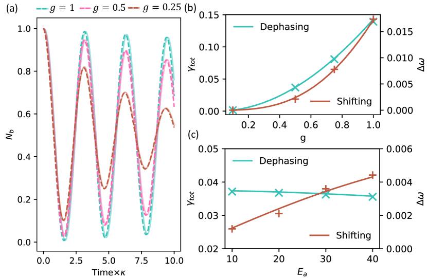
Figure 1: Comparison between numerical simulation results and analytical prediction of quantum frequency conversion. Here, the parameters for all the results are $\kappa_{a}=20$, $E_{a}=20$, and $g=0.5$. (a) The evolution of photon population of mode $b$ under various $g$, with a fixed $G$ via full model (solid lines) and $H_{\mathrm{MFT}}$ with extra operators (dashed lines). (b) The dissipation rate and frequency shift (solid line) under various $g$ and fixed $E_{a}$ and $\kappa_{a}$ compared with simulation results (cross). (c) The dephasing rate and frequency shift (solid line) under various $E_{a}$ and fixed $g$ and $\kappa_{a}$ compared with simulation results (cross).

The validity of the MFPT is also tested by considering the indicator for the amplitude of subsystem A. As pointed out above, the mean-field $\alpha$ of mode $a$ might not be solved independently if the coupling strength $g$ or excitation numbers in mode $b,c$ is strong enough, as the backaction from subsystem B would affect the mean-field of mode $a$ in practical experiments. Considering the practical frequency conversion experiments with a coherent signal input $E_{b}(b^{\dagger}+b)$ to mode $b$, and thus we have

$$\mathscr{I}[a]_{1} =\frac{4E_{b}^{2}g^{2}}{\left(\frac{\kappa_{b}}{2}+\frac{2|G|^{2}}{\kappa_{c}}\right)^{2}\kappa_{a}\kappa_{c}}.$$

As expected, larger $E_{a}$ ($G\propto gE_{a}$) and smaller $E_{b}$ lead to a smaller $\mathscr{I}[a]_{1}$, i.e. a better approximation of $H_{\mathrm{MFT}}$. As shown in Fig. 2(a), we see that the indicator decreases monotonously with $E_{a}$ if we fix $G$, i.e. $g\propto 1/E_{a}$. While for small pump power $E_{a}$ (shadow area), the indicator grows extremely large and the MFT shall fail here. The numerical results are obtained using the quantum cluster expansion (QCE) method and Fock state truncation (FST) by Qutip (huang2021classical, ; johansson2012qutip, ). The deviation between the indicator and the results of QCE and FST demonstrate such a statement. We can see from Fig. 2(b) that the indicator fits well with the simulation with small discrepancy. It justifies the argument that for strong coupling strength $g$, a sufficiently large $E_{a}$ is necessary to ensure the accuracy of traditional MFT.

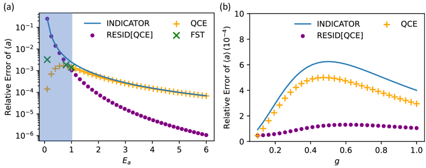
Figure 2: The indicator by the analytical prediction (blue solid line) and the numerical simulation via quantum cluster expansion (QCE) method (orange cross) and Fock state truncation (FST, green cross) under asymmetric MFPT. The purple dot corresponds to the residual error between the analytical results and the results from QCE. The relative error is defined by $\textrm{Relative Error of }\langle R\rangle\triangleq\left|\frac{\langle R\rangle_{simu}-\langle R\rangle_{MFT}}{\langle R\rangle_{MFT}}\right|,$ where $\langle R\rangle_{simu}$ is the value given by full model simulation and $\langle R\rangle_{MFT}$ is the value given by the MFT. (a) The indicators under various drive strength of mode $a$ with fixed $G=-i$ and the shadow area indicates the parameter region where asymmetric first-order MFPT may fail. (b) The indicators under various $g$ with a fixed pump strength $E_{a}=2$. In both cases, $\kappa_{a}=\kappa_{b}=\kappa_{c}=2$ and $E_{b}=0.1$ are fixed.

IV.2 Symmetric MFPT

Lastly, we provide an example of symmetric MFPT. All the above analyses are focusing on an asymmetric system with $E_{a}\gg E_{b}$ to give a precise description of the system. In principle, adapting the asymmetric MFPT can also describe the backward perturbation from subsystem B to A when applying the perturbation theory to high orders. While the calculation of the higher-order perturbations is cumbersome in practice due to the existence of the first-order perturbation terms in subsystem A. By treating the two subsystems on the same footing, symmetric MFPT helps include all the mean-field influences between two subsystems and extract the correction induced by the correlations to the higher-order, which is quite suitable for investigating the case that $E_{b}$ is comparable to $E_{a}$. For the symmetric MFPT

$$H_{\mathrm{MFT}}= g(\alpha^{*}bc^{\dagger}+\alpha bc)+E_{a}(a^{\dagger}+a)$$

$$+g\left(a^{\dagger}\langle bc^{\dagger}\rangle_{0}+a\langle b^{\dagger}c\rangle_{0}\right)+E_{b}(b^{\dagger}+b),$$ (21)

the mean-field value of $a$ is the solution of the cubic equation

$$\alpha=-iE_{a}+\frac{E_{b}^{2}g^{2}\alpha}{(1+|\alpha|^{2}g^{2})^{2}},$$ (22)

where we assume $\kappa_{a}=\kappa_{b}=\kappa_{c}=2$ for simplicity in the following calculation. According to Eq. (7), the first order indicators for both subsystems are zero and we follow the same process to calculate the second-order indicators as

$$\mathscr{\mathscr{I}}[a]_{2} =\left|\frac{-ig\langle bc^{\dagger}\rangle_{1,ss}}{\langle a\rangle_{0,ss}}\right|=0$$ (23)

$$\mathscr{I}[b]_{2} =\mathscr{I}[c]_{2}=\left|\frac{2g^{2}}{(1+|\alpha|^{2}g^{2})(4-g^{2}|\alpha|^{2})}\right|.$$ (24)

It can be seen directly that the symmetric MFPT is a third-order approximation for mode $a$ and thus the MFPT is efficient for subsystem A as long as the pump is large enough. As shown in Fig. 3, the proposed theory agrees quite well with the simulation of the relative error..

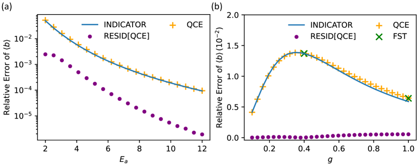
Figure 3: The indicator (solid line) compared to the simulation result of the relative error via quantum cluster expansion (QCE) method (orange cross) and Fock state truncation (FST, green cross) under symmetric MFPT. The purple dot corresponds to the residual between Indicator and QCE. The relative error is defined by $\textrm{Relative Error of }\langle R\rangle\triangleq\left|\frac{\langle R\rangle_{simu}-\langle R\rangle_{MFT}}{\langle R\rangle_{MFT}}\right|,$ where $\langle R\rangle_{simu}$ is the value given by full model simulation and $\langle R\rangle_{MFT}$ is the value given by the MFT. (a) Results against $E_{a}$, with fixed coupling strength $g=1$. (b) Results against coupling strength $g$, with fixed drive amplitude $E_{a}=4$. In both cases, $\kappa_{a}=\kappa_{b}=\kappa_{c}=2$ and $E_{b}=0.1$ are fixed.

V Conclusion

In summary, a general approach combining the MFT and the perturbation theory is developed to extract the quantum correlation-induced effects beyond the MFT in quantum optics systems. Upon the traditional MFT, which separates the system into two subsystems and neglects the correlation between them, we derive the additional decoherence effects and modification of Hamiltonian to provide a more precise description of the quantum system. Furthermore, indicators are provided to quantitatively measure the accuracy of MFT. Via a practical quantum optics model of frequency conversion, our approach is validated by comparing with numerical simulations based on the full Hamiltonian. The indicators as well as the extra super-operators derived by our approach help us design the system parameters so that the unwanted effects could be suppressed and optimal quantum operation fidelity could be achieved in experiments. Our approach provides a general framework of the MFT, and the choice of MFT Hamiltonian enjoys a high degree of freedom, which may give rise to rich possibilities of extracting the appreciable evolution beyond the mean-value. Further extension of the approach to divide the system into more subsystems and the applications in designing quantum devices are potential research topics for future works.

- (1) H. Stanley, Mean field theory of magnetic phase transitions, Introduction to Phase Transitions and Critical Phenomena (1971).
- (2) L. P. Kadanoff, More is the same; phase transitions and mean field theories, Journal of Statistical Physics 137, 777 (2009).
- (3) N. N. Bogolyubov, A method for studying model Hamiltonians: a minimax principle for problems in statistical physics, volume 43 (Elsevier 2013).
- (4) A. Blais, R.-S. Huang, A. Wallraff, S. M. Girvin, and R. J. Schoelkopf, Cavity quantum electrodynamics for superconducting electrical circuits: An architecture for quantum computation, Physical Review A 69, 062320 (2004).
- (5) J. Gea-Banacloche, Some implications of the quantum nature of laser fields for quantum computations, Physical Review A 65, 022308 (2002).
- (6) K. Igeta, N. Imoto, and M. Koashi, Fundamental limit to qubit control with coherent field, Physical Review A 87, 022321 (2013).
- (7) J. Gea-Banacloche, Energy constraints for quantum logic via nonlinear optical processes, Optics communications 283, 719 (2010).
- (8) S. J. van Enk and H. J. Kimble, On the classical character of control fields in quantum information processing, arXiv preprint quant-ph/0107088 (2001).
- (9) D. V. Strekalov, C. Marquardt, A. B. Matsko, H. G. Schwefel, and G. Leuchs, Nonlinear and quantum optics with whispering gallery resonators, Journal of Optics 18, 123002 (2016).
- (10) G. Lindblad, On the generators of quantum dynamical semigroups, Communications in Mathematical Physics 48, 119 (1976).
- (11) X. Yi, C. Li, and J. Su, Perturbative expansion for the master equation and its applications, Physical Review A 62, 013819 (2000).
- (12) M. O. Scully and M. S. Zubairy, Quantum optics (American Association of Physics Teachers 1999).
- (13) E. A. Gómez, J. D. Castaño-Yepes, and S. P. Thirumuruganandham, Perturbation theory for open quantum systems at the steady state, Results in Physics 10, 353 (2018).
- (14) V. Ginzburg, Some remarks on phase transitions of the second kind and the microscopic theory of ferroelectric materials, Soviet Phys. Solid State 2, 1824 (1961).
- (15) Y.-X. Huang, M. Li, K. Lin, Y.-L. Zhang, G.-C. Guo, and C.-L. Zou, Classical-to-quantum transition in multimode nonlinear systems with strong photon-photon coupling, arXiv preprint arXiv:2111.09557 (2021).
- (16) J. R. Johansson, P. D. Nation, and F. Nori, Qutip: An open-source python framework for the dynamics of open quantum systems, Computer Physics Communications 183, 1760 (2012).