font=normalsize

A short course on
Tensor algebra and analysis for engineers
with applications to differential geometry

To Carla, Bianca and Alessandro

Preface

This textbook, addressed to graduate students and young researchers in mechanics, has been developed from the class notes of different courses in continuum mechanics that I have been delivering for several years as part of the Master’s program in MMM - Mathematical Methods for Mechanics, at the University Paris-Saclay.

Far from being exhaustive, as any primer text, the intention of this book is to introduce students in mechanics and engineering to the mathematical language and tools that are necessary for a modern approach to continuum theoretical and applied mechanics. The presentation of the matter is hence tailored for this scientific community and necessarily it is different, in terms of language and objectives, from that normally proposed to students of other disciplines, such as physics, especially general relativity, or pure mathematics.

What has motivated me to write this textbook is the idea of collecting in a single, introductory book a set of results and tools useful for studies in mechanics and presenting them in a modern, succinct way. Almost all the results and theorems are proved and the reader is guided along a tour that starts from vectors and ends at the differential geometry of surfaces, passing through the algebra of tensors of second and fourth orders, the differential geometry of curves, the tensor analysis for fields and deformations and the use of curvilinear coordinates.

Some topics are specially treated, such as rotations, the algebra of fourth order tensors, fundamental for the mechanics of modern materials, or the properties of differential operators. Some other topics are intentionally omitted because they are less important to continuum mechanics or too advanced for an introductory text. Though, in some modern texts, tensors are directly presented in the most general setting of curvilinear coordinates, I preferred here to choose a more traditional approach, introducing first tensors in Cartesian coordinates, normally used for classical problems. Then, an entire chapter is devoted to the passage to curvilinear coordinates and to the formalism of co- and contravariant components.

The tensor theory and results are specially applied to introduce some subjects concerning differential geometry of curves and surfaces. Also in this case, the presentation is mainly intended for applications to continuum mechanics and, in particular, in view of courses on slender beams or thin shells. All the presentation of the topics of differential geometry is extensively based on tensor algebra and analysis.

More than a hundred exercises are proposed to the reader, many of them completing the theoretical part through new results and proofs. All the exercises are entirely developed and solved at the end of the book, in order to provide the reader with thorough support for his learning.

In Chapter 1, vectors and points are introduced and also, with a small anticipation of some results of the second Chapter, also applied vectors are visited. Chapter 2 is completely devoted to the algebra of second-rank tensors and the succeeding Chapter 3 to that of fourth-rank tensors. Intentionally, these are the only two types of tensors introduced in the book: They are the most important types of tensors in mechanics, by them we can represent deformation, stress and the constitutive laws. I preferred not to introduce tensors in an absolutely general way but to go directly to the most important tensors for applications in mechanics; for the same reason, the algebra of other tensors, namely of third-rank tensors, is not presented in this primer text.

The analysis of tensors is first done using differential geometry of curves, in Chapter 4, for differentiation and integration with respect to only one variable, then introducing the differential operators for fields and deformations, in Chapter 5.

Then, a generalization of second-rank tensor algebra and analysis in the sense of the use of curvilinear coordinates is presented in Chapter 6, where the notion of metric tensor, co- and contravariant components and Christoffel’s symbols are introduced.

Finally, Chapter 7 is entirely devoted to an introduction to the differential geometry of surfaces. Classical topics such as the first and second fundamental forms of a surface, the different types of curvatures, the Gauss-Weingarten equations or the concepts of minimal surfaces, geodesics and the Gauss-Codazzi conditions are presented, with all these topics being of a great interest in mechanics.

I tried to write a coherent, almost self-contained manual of mathematical tools for graduate students in mechanics, with the hope of helping young students progress in their studies. The exposition is as simple as possible, sober, sometimes minimalist. I intentionally avoided burdening the language and the text with nonessential details and considerations, but I have always tried to grasp the essence of a result and its usefulness.

It is my most sincere hope that the reader who dares to persevere through the pages of this book will find a benefit for his studies in continuum mechanics. This is, eventually, the goal of this primer text.

Versailles, June 16, 2022

List of symbols

$:=$ : definition symbol
$|$: such that
$\exists!$: exists and is unique
$\mathbb{R}$: set of real numbers
$\mathcal{E}$: ordinary 3D Euclidean space
$\mathcal{V}$: vector space of translations, associated with $\mathcal{E}$
$Lin(\mathcal{V})$: vector space of second-rank tensors
$\mathbb{L}$in$(\mathcal{V})$: vector space of fourth-rank tensors
$x,y,z$ etc.: scalars (elements of $\mathbb{R}$)
$p,q,r$ etc.: points (elements of $\mathcal{E}$)
$\mathbf{u},\mathbf{v},\mathbf{w}$ etc.: vectors (elements of $\mathcal{V}$)
$\mathbf{u}=p-q$ etc.: vector difference of two points of $\mathcal{E}$
$\mathbf{L},\mathbf{M},\mathbf{N}$ etc.: second-rank tensors (elements of $Lin(\mathcal{V})$)
$\mathbb{L},\mathbb{M},\mathbb{N}$ etc.: fourth-rank tensors (elements of $\mathbb{L}$in$(\mathcal{V})$)
$\mathbf{u}\cdot\mathbf{v}$ etc.: scalar product of vectors
$\mathbf{L}\cdot\mathbf{M}$ etc.: scalar product of second-rank tensors
$\mathbf{u}\times\mathbf{v}$ etc.: cross product of vectors
$\mathbf{u}\otimes\mathbf{v}$ etc.: dyad (second-rank tensor) of vectors
$u=|\mathbf{u}|$: norm of a vector
$L=|\mathbf{L}|$: norm of a tensor
$|p-q|,|\mathbf{u}-\mathbf{v}|,|\mathbf{L}-\mathbf{M}|$: distance of points, vectors or tensors
$\det\mathbf{L}$: determinant of a second-rank tensor $\mathbf{L}$
$\mathbf{L}^{\top}$: transpose of a second-rank tensor $\mathbf{L}$
$\mathbf{L}^{-1}$: inverse of a second-rank tensor $\mathbf{L}$
$\mathbf{L}^{-\top}=(\mathbf{L}^{\top})^{-1}=(\mathbf{L}^{-1})^{\top}$
$Sym(\mathcal{V})$: subspace of $Lin(\mathcal{V})$ of symmetric second-rank tensors
$Skw(\mathcal{V})$: subspace of $Lin(\mathcal{V})$ of skew second-rank tensors
$Sph(\mathcal{V})$: subspace of $Lin(\mathcal{V})$ of spherical second-rank tensors
$Dev(\mathcal{V})$: subspace of $Lin(\mathcal{V})$ of deviatoric second-rank tensors
$Orth(\mathcal{V})$: subspace of $Lin(\mathcal{V})$ of orthogonal second-rank tensors
$Orth(\mathcal{V})^{+}$: subspace of $Lin(\mathcal{V})$ of rotation second-rank tensors
$\mathcal{S}$: unit sphere of $\mathcal{V}$: $\mathcal{S}=\{\mathbf{u}\in\mathcal{V}|\ |\mathbf{u}|=1\}$
$\delta_{ij}$: Kronecker’s delta
$\Re$: real part of a complex quantity
$\Im$: imaginary part of a complex quantity
$\mathbb{L}=\mathbf{A}\boxtimes\mathbf{B}$: conjugation product of two second-rank tensors
$\mathbb{S}^{sph}$: spherical projector
$\mathbb{D}^{dev}$: deviatoric projector
$\mathbb{T}^{trp}$: transpose projector
$\mathbb{S}^{sym}$: symmetry projector
$\mathbb{W}^{skw}$: antisymmetry projector
$\mathbb{I}$: identity of $\mathbb{L}$in($\mathcal{V}$)
$\mathbb{I}^{s}$: restriction of $\mathbb{I}$ to symmetric tensors of $Lin(\mathcal{V})$

Contents

1. Preface
2. List of symbols
3. 1 Points and vectors
   1. 1.1 Points and vectors
   2. 1.2 Scalar product, distance, orthogonality
   3. 1.3 Basis of $\mathcal{V}$, expression of the scalar product
   4. 1.4 Applied vectors
   5. 1.5 Exercises
4. 2 Second rank tensors
   1. 2.1 Second-rank tensors
   2. 2.2 Dyads, tensor components
   3. 2.3 Tensor product
   4. 2.4 Transpose, symmetric and skew tensors
   5. 2.5 Trace, scalar product of tensors
   6. 2.6 Spherical and deviatoric parts
   7. 2.7 Determinant, inverse of a tensor
   8. 2.8 Eigenvalues and eigenvectors of a tensor
   9. 2.9 Skew tensors and cross product
   10. 2.10 Orientation of a basis
   11. 2.11 Rotations
   12. 2.12 Reflexions
   13. 2.13 Polar decomposition
   14. 2.14 Exercises
5. 3 Fourth rank tensors
   1. 3.1 Fourth-rank tensors
   2. 3.2 Dyads, tensor components
   3. 3.3 Conjugation product, transpose, symmetries
   4. 3.4 Trace and scalar product of fourth-rank tensors
   5. 3.5 Projectors, identities
   6. 3.6 Orthogonal conjugator
   7. 3.7 Rotations and symmetries
   8. 3.8 The Kelvin formalism
   9. 3.9 The polar formalism for plane tensors
   10. 3.10 Exercises
6. 4 Tensor analysis: curves
   1. 4.1 Curves of points, vectors and tensors
   2. 4.2 Differention of curves
   3. 4.3 Integral of a curve of vectors and length of a curve
   4. 4.4 The Frenet-Serret basis
   5. 4.5 Curvature of a curve
   6. 4.6 The Frenet-Serret formulae
   7. 4.7 The torsion of a curve
   8. 4.8 Osculating sphere and circle
   9. 4.9 Evolute, involute and envelopes of plane curves
   10. 4.10 The theorem of Bonnet
   11. 4.11 Canonic equations of a curve
   12. 4.12 Exercises
7. 5 Tensor analysis: fields
   1. 5.1 Scalar, vector and tensor fields
   2. 5.2 Differentiation of fields, differential operators
   3. 5.3 Properties of the differential operators
   4. 5.4 Theorems on fields
   5. 5.5 Differential operators in Cartesian coordinates
   6. 5.6 Differential operators in cylindrical coordinates
   7. 5.7 Differential operators in spherical coordinates
   8. 5.8 Exercises
8. 6 Curvilinear coordinates
   1. 6.1 Introduction
   2. 6.2 Curvilinear coordinates, metric tensor
   3. 6.3 Co- and contra-variant components
   4. 6.4 Spatial derivatives of fields in curvilinear coordinates
   5. 6.5 Exercises
9. 7 Surfaces in $\mathcal{E}$
   1. 7.1 Surfaces in $\mathcal{E}$, coordinate lines, tangent planes
   2. 7.2 Surfaces of revolution
   3. 7.3 Ruled surfaces
   4. 7.4 First fundamental form of a surface
   5. 7.5 Second fundamental form of a surface
   6. 7.6 Curvatures of a surface
   7. 7.7 The theorem of Rodrigues
   8. 7.8 Classification of the points of a surface
   9. 7.9 Developable surfaces
   10. 7.10 Points of a surface of revolution
   11. 7.11 Lines of curvature, conjugated directions, asymptotic directions
   12. 7.12 The Dupin’s conical curves
   13. 7.13 The Gauss-Weingarten equations
   14. 7.14 The Theorema Egregium
   15. 7.15 Minimal surfaces
   16. 7.16 Geodesics
   17. 7.17 The Gauss-Codazzi compatibility conditions
   18. 7.18 Exercises

Chapter 1 Points and vectors

1.1 Points and vectors

We consider in the following a point space $\mathcal{E}$, whose elements are points $p$. In classical mechanics, $\mathcal{E}$ is to be identified with the Euclidean three-dimensional space, wherein events are intended to be set. On $\mathcal{E}$, we admit the existence of an operation, the difference of any couple of its elements:

$$q-p,\ \ p,q\in\mathcal{E}.$$

We associate to $\mathcal{E}$ a vector space $\mathcal{V}$ whose dimension is dim$\mathcal{V}=3$ and whose elements are vectors $\mathbf{v}$ representing translations over $\mathcal{E}$:

$$\forall p,q\in\mathcal{E},\ \exists!\ \mathbf{v}\in\mathcal{V}|\ q-p=\mathbf{v}.$$

Any element $\mathbf{v}\in\mathcal{V}$ is hence a transformation over $\mathcal{E}$ that, using the previous definition, can be written as :

$$\forall\mathbf{v}\in\mathcal{V},\ \mathbf{v}:\mathcal{E}\rightarrow\mathcal{E}|\ q=\mathbf{v}(p)\ \rightarrow\ q=p+\mathbf{v}.$$

We remark that the result of the application of the translation $\mathbf{v}$ depends upon the argument $p$:

$$q=p+\mathbf{v}\neq p_{1}+\mathbf{v}=q_{1},$$

whose geometric meaning is depicted in Fig. 1.1. Unlike difference, the sum of two points is not defined and is meaningless.

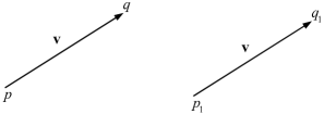
Figure 1.1: Same translation applied to two different points.

We define the sum of two vectors $\mathbf{u}$ and $\mathbf{v}$ as the vector $\mathbf{w}$ such that

$$(\mathbf{u}+\mathbf{v})(p)=\mathbf{u}(\mathbf{v}(p))=\mathbf{w}(p)$$

This means that, if

$$q=\mathbf{v}(p)=p+\mathbf{v},$$

then

$$r=\mathbf{u}(q)=q+\mathbf{u}=\mathbf{w}(p),$$

see Fig. 1.2, which shows that the above definition actually coincides with the parallelogram rule and that

$$\mathbf{u}+\mathbf{v}=\mathbf{v}+\mathbf{u},$$

as obvious, for the sum over a vector space commutes. It is evident that the sum of more than two vectors can be defined iteratively, summing up a vector at a time to the sum of the previous vectors.

The null vector $\mathbf{o}$ is defined as the difference of any two coincident points:

$$\mathbf{o}:=p-p\ \ \forall p\in\mathcal{E};$$

$\mathbf{o}$ is unique and the only vector such that

$$\mathbf{v}+\mathbf{o}=\mathbf{v}\ \ \forall\mathbf{v}\in\mathcal{V}.$$

Figure 1.2: Sum of two vectors: the parallelogram rule.

In fact,

$$\forall p\in\mathcal{E},\ \ \mathbf{v}+\mathbf{o}=\mathbf{v}+p-p\ \rightarrow\ p+\mathbf{v}+\mathbf{o}=p+\mathbf{v}\ \iff\ \mathbf{v}+\mathbf{o}=\mathbf{v}.$$

A linear combination of $n$ vectors $\mathbf{v}_{i}$ is defined as the vector

$$\mathbf{w}:=k_{i}\mathbf{v}_{i},\ \ k_{i}\in\mathbb{R},\ \ i=1,...,n.$$

The $n+1$ vectors $\mathbf{w},\ \mathbf{v}_{i},\ i=1,...,n,$ are said to be linear independent if there does not exist a set of $n$ scalars $k_{i}$ such that the above equation is satisfied and are said to be linear dependent in the opposite case.

1.2 Scalar product, distance, orthogonality

A scalar product on a vector space is a positive definite, symmetric, bilinear form. A form $\omega$ is a function

$$\omega:\mathcal{V}\times\mathcal{V}\rightarrow\mathbb{R},$$

i.e. $\omega$ operates on a couple of vectors to give a real number, a scalar. We will indicate the scalar product of two vectors $\mathbf{u}$ and $\mathbf{v}$ as

$$\omega(\mathbf{u},\mathbf{v})=\mathbf{u}\cdot\mathbf{v}.$$

The properties of bilinearity prescribe that, $\forall\mathbf{u},\mathbf{v}\in\mathcal{V}$ and $\forall\alpha,\beta\in\mathbb{R}$,

$$\begin{split}&\mathbf{u}\cdot(\alpha\mathbf{v}+\beta\mathbf{w})=\alpha\mathbf{u}\cdot\mathbf{v}+\beta\mathbf{u}\cdot\mathbf{w},\\ &(\alpha\mathbf{u}+\beta\mathbf{v})\cdot\mathbf{w}=\alpha\mathbf{u}\cdot\mathbf{w}+\beta\mathbf{v}\cdot\mathbf{w},\end{split}$$

while symmetry implies that

$$\mathbf{u}\cdot\mathbf{v}=\mathbf{v}\cdot\mathbf{u}\ \ \forall\mathbf{u},\mathbf{v}\in\mathcal{V}.$$

Finally, the positive definiteness means that

$$\mathbf{v}\cdot\mathbf{v}>0\ \ \forall\mathbf{v}\in\mathcal{V},\ \ \mathbf{v}\cdot\mathbf{v}=0\ \iff\ \mathbf{v}=\mathbf{o}.$$

Any two vectors $\mathbf{u},\mathbf{v}\in\mathcal{V}$ are said to be orthogonal $\iff$

$$\mathbf{u}\cdot\mathbf{v}=0.$$

Thanks to the properties of the scalar product, we can define the Euclidean norm of a vector $\mathbf{v}$ as the nonnegative scalar, denoted equivalently by $v$ or $|\mathbf{v}|$,

$$v=|\mathbf{v}|:=\sqrt{\mathbf{v}\cdot\mathbf{v}}$$

Theorem 1.

The norm of a vector has the following properties: $\forall\mathbf{u},\mathbf{v}\in\mathcal{V},k\in\mathbb{R}$,

$$\begin{split}&|\mathbf{u}\cdot\mathbf{v}|\leq u\ v\ \ \mathrm{(Schwarz^{\prime}s\ inequality)};\\ &|\mathbf{u}+\mathbf{v}|\leq u+v\ \ \mathrm{(Minkowski^{\prime}s\ triangular\ inequality)};\\ &|k\mathbf{v}|=|k|v.\end{split}$$

Proof.

Schwarz’s inequality: It is sufficient to prove that

$$(\mathbf{u}\cdot\mathbf{v})^{2}\leq\mathbf{u}\cdot\mathbf{u}\ \mathbf{v}\cdot\mathbf{v}.$$

Let $x=\mathbf{v}\cdot\mathbf{v}$ and $y=-\mathbf{u}\cdot\mathbf{v}$. Then, by the positive definiteness of the scalar product, we get

$$(x\mathbf{u}+y\mathbf{v})\cdot(x\mathbf{u}+y\mathbf{v})\geq 0,$$

which implies that

$$x^{2}\mathbf{u}\cdot\mathbf{u}+2xy\mathbf{u}\cdot\mathbf{v}+y^{2}\mathbf{v}\cdot\mathbf{v}=(\mathbf{v}\cdot\mathbf{v})^{2}\mathbf{u}\cdot\mathbf{u}-2\mathbf{v}\cdot\mathbf{v}(\mathbf{u}\cdot\mathbf{v})^{2}+\mathbf{v}\cdot\mathbf{v}(\mathbf{u}\cdot\mathbf{v})^{2}\geq 0;$$

supposing $\mathbf{v}\neq\mathbf{o}$ (otherwise, the proof is trivial), we get the thesis on dividing by $\mathbf{v}\cdot\mathbf{v}$.

Minkowski’s inequality: Because the two members of the inequality to be proved are nonnegative, it is sufficient to prove that

$$(\mathbf{u}+\mathbf{v})\cdot(\mathbf{u}+\mathbf{v})\leq(u+v)^{2}=u^{2}+2uv+v^{2}.$$

This can be proved easily:

$$\begin{split}(\mathbf{u}+\mathbf{v})\cdot(\mathbf{u}+\mathbf{v})&=\mathbf{u}\cdot\mathbf{u}+2\mathbf{u}\cdot\mathbf{v}+\mathbf{v}\cdot\mathbf{v}=u^{2}+2\mathbf{u}\cdot\mathbf{v}+v^{2}\\ &\leq u^{2}+2|\mathbf{u}\cdot\mathbf{v}|+v^{2}\leq u^{2}+2uv+v^{2},\end{split}$$

in which the last operation follows from the Schwarz’s inequality.

The proof of the third property is immediate, it is sufficient to use the same definition of norm. ∎

We define distance between any two points $p$ and $q\ \in\mathcal{E}$ the scalar

$$d(p,q):=|p-q|=|q-p|.$$

Similarly, the distance between two any vectors $\mathbf{u}$ and $\mathbf{v}\ \in\mathcal{V}$ is defined as

$$d(\mathbf{u},\mathbf{v}):=|\mathbf{u}-\mathbf{v}|=|\mathbf{v}-\mathbf{u}|.$$

Two points or two vectors are coincident if and only if their distance is null.

The unit sphere $\mathcal{S}$ of $\mathcal{V}$ is defined as the set of all the vectors whose norm is one:

$$\mathcal{S}:=\{\mathbf{v}\in\mathcal{V}|\ v=1\}.$$

1.3 Basis of $\mathcal{V}$, expression of the scalar product

There is a general way to define a basis for a vector space of any kind. Here, we limit the introduction of the concept of basis to the case of $\mathcal{V}$ only, of interest in classical mechanics. Generally speaking, a basis $\mathcal{B}$ of $\mathcal{V}$ is any set of three linearly independent vectors $\mathbf{e}_{i},i=1,2,3$ of $\mathcal{V}$:

$$\mathcal{B}=\{\mathbf{e}_{1},\mathbf{e}_{2},\mathbf{e}_{3}\}.$$

The introduction of a basis for $\mathcal{V}$ is useful for representing vectors. In fact, once a basis $\mathcal{B}$ is fixed, any vector $\mathbf{v}\in\mathcal{V}$ can be represented as a linear combination of the vectors of the basis, where the coefficients $v_{i}$ of the linear combination are the Cartesian components of $\mathbf{v}$:

$$\mathbf{v}=v_{i}\mathbf{e}_{i}=v_{1}\mathbf{e}_{1}+v_{2}\mathbf{e}_{2}+v_{3}\mathbf{e}_{3}.$$

Though the choice of the elements of a basis is completely arbitrary, the only condition being their linear independency, we will use in the following only orthonormal bases, which are bases composed of mutually orthogonal vectors of $\mathcal{S}$, i.e. satisfying

$$\mathbf{e}_{i}\cdot\mathbf{e}_{j}=\delta_{ij},$$

where the symbol $\delta_{ij}$ is the so-called Kronecker’s delta:

$$\delta_{ij}=\left\{\begin{split}&1\ \mathrm{if}\ i=j,\\ &0\ \mathrm{if}\ i\neq j.\end{split}\right.$$

The use of orthonormal bases has great advantages; namely, it allows us to give a very simple rule for the calculation of the scalar product:

$$\mathbf{u}\cdot\mathbf{v}=u_{i}\mathbf{e}_{i}\cdot v_{j}\mathbf{e}_{j}=u_{i}v_{j}\delta_{ij}=u_{i}v_{i}=u_{1}v_{1}+u_{2}v_{2}+u_{3}v_{3}.$$

In particular, it is

$$\mathbf{v}\cdot\mathbf{e}_{i}=v_{k}\mathbf{e}_{k}\cdot\mathbf{e}_{i}=v_{k}\delta_{ik}=v_{i},\ \ i=1,2,3.$$

So, the Cartesian components of a vector are the projection of the vector on the three vectors of the basis $\mathcal{B}$; such quantities are the director cosines of $\mathbf{v}$ in the basis $\mathcal{B}$. In fact, if $\theta$ is the angle formed by two vectors $\mathbf{u}$ and $\mathbf{v}$, then

$$\mathbf{u}\cdot\mathbf{v}=u\ v\ \cos\theta.$$

This relation is used to define the angle between two vectors,

$$\theta=\arccos\frac{\mathbf{u}\cdot\mathbf{v}}{u\ v},$$

which can be proved easily: Given two vectors $\mathbf{u}$ and $\mathbf{v}$, we look for $c\in\mathbb{R}$ such that the vector $\mathbf{u}-c\mathbf{v}$ is orthogonal to $\mathbf{v}$:

$$(\mathbf{u}-c\mathbf{v})\cdot\mathbf{v}=0\ \iff\ c=\frac{\mathbf{u}\cdot\mathbf{v}}{\mathbf{v}\cdot\mathbf{v}}=\frac{\mathbf{u}\cdot\mathbf{v}}{v^{2}}.$$

Now, if $\mathbf{u}$ is inclined of $\theta$ on $\mathbf{v}$, its projection $u_{v}$ on the direction of $\mathbf{v}$ is

$$u_{v}=u\ \cos\theta,$$

and, by construction (see Fig. 1.3), it is also

$$u_{v}=c\ v.$$

So,

$$c=\frac{u}{v}\cos\theta\ \rightarrow\ \frac{u}{v}\cos\theta=\frac{\mathbf{u}\cdot\mathbf{v}}{v^{2}}\ \Rightarrow\ \cos\theta=\frac{\mathbf{u}\cdot\mathbf{v}}{u\ v}.$$

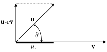
Figure 1.3: Angle between two vectors.

We remark that while the scalar product, being an intrinsic operation, does not change for a change of basis, the components $v_{i}$ of a vector are not intrinsic quantities, but they are basis-dependent: A change of the basis makes the components change. The way this change is done will be introduced in Section 2.11.

A frame $\mathcal{R}$ for $\mathcal{E}$ is composed of a point $o\in\mathcal{E}$, the origin, and a basis $\mathcal{B}$ of $\mathcal{V}$:

$$\mathcal{R}:=\{o,\mathcal{B}\}=\{o;\mathbf{e}_{1},\mathbf{e}_{2},\mathbf{e}_{3}\}.$$

The use of a frame for $\mathcal{E}$ is useful for determining the position of a point $p$, which can be done through its Cartesian coordinates $x_{i}$, defined as the components in $\mathcal{B}$ of the vector $p-o$:

$$x_{i}:=(p-o)\cdot\mathbf{e}_{i},\ \ i=1,2,3.$$

Of course, the coordinates $x_{i}$ of a point $p\in\mathcal{E}$ depend upon the choice of $o$ and $\mathcal{B}$.

1.4 Applied vectors

We introduce now a set of definitions, concepts and results that are widely used in physics, especially in mechanics. For that, we need to anticipate some results that are introduced in the next Chapter, namely that of cross product, in Section 2.9, and of complementary projector, in Exercise 2, Chapter 2. This slight deviation from the good rule of consistent progression in stating the results is justified by the fact that, actually, the matter exposed hereafter is still that of vectors. The readers can, of course, come back to the topics of this section once they have studied Chapter 2.

We call applied vector $\mathbf{v}^{p}$ a vector $\mathbf{v}$ associated to a point $p\in\mathcal{E}$. In physics the concept of applied vector is often employed, for example, to represent forces. We define the resultant of a system of $n$ applied vectors $\mathbf{v}^{p}_{i}$ as the vector

$$\mathbf{R}:=\sum_{i=1}^{n}\mathbf{v}^{p}_{i}.$$

We define moment of an applied vector $\mathbf{v}^{p}$ about a point $o$, called the center of the moment, the vector

$$\mathbf{M}_{o}:=(p-o)\times\mathbf{v}^{p},$$

and resultant moment of a system of $n$ applied vectors $\mathbf{v}^{p}_{i}$ about a point $o$ the vector

$$\mathbf{M}^{r}_{o}:=\sum_{i=1}^{n}(p_{i}-o)\times\mathbf{v}^{p}_{i}.$$

We remark that $\mathbf{R},\mathbf{M}_{o}$ and $\mathbf{M}^{r}_{o}$ are not applied vectors.

If $\mathbf{u}\in\mathcal{S}|\ \mathbf{u}\times\mathbf{v}^{p}=\mathbf{o}$, then

$$b:=|(\mathbf{I}-\mathbf{u}\otimes\mathbf{u})(p-o)|=|p-o|\sin\theta$$

is called the moment arm of $\mathbf{v}^{p}$ with respect to the center $o$. It measures the distance of $o$ from the line of action, i.e. the line passing through $p$ and parallel to $\mathbf{v}^{p}$, cf. Fig. 1.4.

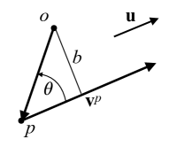
Figure 1.4: Moment arm of an applied vector.

Theorem 2.

(Transport of the moment). If $\mathbf{M}_{o_{1}}$ is the moment of an applied vector $\mathbf{v}^{p}$ about a center $o_{1}$, the moment $\mathbf{M}_{o_{2}}$ of $\mathbf{v}^{p}$ about to another center $o_{2}$ is

$$\mathbf{M}_{o_{2}}=\mathbf{M}_{o_{1}}+(o_{1}-o_{2})\times\mathbf{v}^{p}.$$

Proof.

Referring to Fig. 1.5,

$$\begin{split}\mathbf{M}_{o_{2}}&=(p-o_{2})\times\mathbf{v}^{p}=(p-o_{1}+o_{1}-o_{2})\times\mathbf{v}^{p}\\ &=(p-o_{1})\times\mathbf{v}^{p}+(o_{1}-o_{2})\times\mathbf{v}^{p}\\ &=\mathbf{M}_{o_{1}}+(o_{1}-o_{2})\times\mathbf{v}^{p}.\end{split}$$

∎

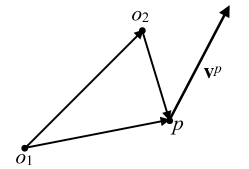
Figure 1.5: Scheme for the transposition of the moment.

A consequence of this theorem is that $\mathbf{M}_{o_{1}}=\mathbf{M}_{o_{2}}\iff\mathbf{v}^{p}\times(o_{1}-o_{2})$, i.e. if $\mathbf{v}^{p}$ and $o_{1}-o_{2}$ are parallel. It follows from this that the moment of an applied vector does not change when calculated about the points of a straight line parallel to the vector itself or, more importantly, if $\mathbf{v}^{p}$ is translated along its line of action.

The above theorem can be extended to the resultant moment of a system of applied vectors to give (the proof is quite similar)

$$\mathbf{M}^{r}_{o_{2}}=\mathbf{M}^{r}_{o_{1}}+(o_{1}-o_{2})\times\mathbf{R}.$$ (1.1)

Also in this case, the resultant moment does not change when $\mathbf{R}$ and $o_{1}-o_{2}$ are parallel vectors, but not exclusively, as another possibility is that $\mathbf{R}=\mathbf{o}$: For the systems of applied vectors with null resultant, the resultant moment is invariant with respect to the center of the moment.

An interesting relation can be found if the two members of the last equation are projected onto $\mathbf{R}$, which gives

$$\mathbf{M}^{r}_{o_{1}}\cdot\mathbf{R}=\mathbf{M}^{r}_{o_{2}}\cdot\mathbf{R}:$$ (1.2)

The projection of the resultant moment onto the direction of $\mathbf{R}$ does not depend upon the center of the moment.

A particularly important case of system with null resultant is that of a couple, which is composed by two opposite vectors $\mathbf{v},-\mathbf{v}$, applied to two points $p$ and $q$:

$$\mathbf{v}^{p}=-\mathbf{v}^{q}.$$

Of course, by definition, $\mathbf{R}=\mathbf{o}$ for any couple and, as a consequence, the resultant moment $\mathbf{M}^{r}$ of a couple, called the moment of the couple and simply denoted by $\mathbf{M}$, is independent of the center of the moment (that is why the index denoting the center of the moment is omitted): Referring to Fig. 1.6,

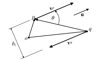
Figure 1.6: Scheme of a couple.

$$\begin{split}\mathbf{M}&=(p-o)\times\mathbf{v}^{p}+(q-o)\times\mathbf{v}^{q}=(p-o)\times\mathbf{v}-(q-o)\times\mathbf{v}\\ &=((p-o)-(q-o))\times\mathbf{v}=(p-q)\times\mathbf{v}.\end{split}$$

If $\mathbf{u}\in\mathcal{S}|\ \mathbf{u}\times\mathbf{v}=\mathbf{o}$, then

$$b_{c}:=|(\mathbf{I}-\mathbf{u}\otimes\mathbf{u})(p-q)|=|p-q|\sin\theta$$

is the couple arm. We then have

$$M=|(p-q)\times\mathbf{v}|=|p-q|v\sin\theta=b_{c}v.$$

The central axis $\mathbf{A}$ of a system of $n$ applied vectors with $\mathbf{R}\neq\mathbf{o}$ is the axis such that

$$\mathbf{M}^{r}_{a}\times\mathbf{R}=\mathbf{o}\ \ \ \forall a\in\mathcal{A}.$$

Theorem 3.

(Existence and uniqueness of the central axis). The central axis of a system of $n$ vectors exists and is unique.

Proof.

Existence: We need at least a point $a\in\mathcal{E}|\ \mathbf{M}^{r}_{a}=k\mathbf{R},\ \ k\in\mathbb{R}\Rightarrow\mathbf{M}^{r}_{a}\times\mathbf{R}=\mathbf{o}$. From Eq. (1.1), $\forall o\in\mathcal{E}$ we get

$$\mathbf{M}^{r}_{a}\times\mathbf{R}=\mathbf{M}^{r}_{o}\times\mathbf{R}+((o-a)\times\mathbf{R})\times\mathbf{R}=\mathbf{M}^{r}_{o}\times\mathbf{R}-\mathbf{R}^{2}(o-a)+(\mathbf{R}\cdot(o-a))\mathbf{R}.$$

Then, if we take for $o-a$ the vector

$$o-a=\frac{\mathbf{M}^{r}_{o}\times\mathbf{R}}{\mathbf{R}^{2}},$$

it is evident that we get

$$\mathbf{M}^{r}_{a}\times\mathbf{R}=\mathbf{o}.$$

Hence, the point

$$a=o-\frac{\mathbf{M}^{r}_{o}\times\mathbf{R}}{\mathbf{R}^{2}}\ \in\mathcal{A}.$$

So, because $\mathbf{M}^{r}$ does not change when calculated with respect to the points of an axis parallel to $\mathbf{R}$, $\mathcal{A}$ is the axis passing through $a$ and parallel to $\mathbf{R}$. Its equation is

$$p=a+t\ \mathbf{R}=o-\frac{\mathbf{M}^{r}_{o}\times\mathbf{R}}{\mathbf{R}^{2}}+t\ \mathbf{R},\ \ \ t\in\mathbb{R}.$$

Uniqueness: Suppose another axis $\hat{\mathcal{A}}\neq\mathcal{A}$ exists, which is necessarily parallel to $\mathcal{A}$. If $q\in\hat{\mathcal{A}}$, again using Eq. (1.1) we get

$$\mathbf{M}^{r}_{q}\times\mathbf{R}=\mathbf{M}^{r}_{a}\times\mathbf{R}+((a-q)\times\mathbf{R})\times\mathbf{R}.$$

In this equation the left-hand side and the first term on the right-hand side are null by the definition of central axis. Because $(a-q)\times\mathbf{R}$ is perpendicular to $\mathbf{R}$ and $\mathbf{R}\neq\mathbf{o}$ by hypothesis, the left-hand side is null if and only if $a=q\Rightarrow\hat{\mathcal{A}}=\mathcal{A}$. ∎

The central axis has another remarkable property:

Theorem 4.

(Property of minimum of the central axis). The points of the central axis minimize the resultant moment.

Proof.

When $\mathbf{M}^{r}$ is calculated about a point $a\in\mathcal{A}$, it is parallel to $\mathbf{R}$, which is not the case for any point $q\notin\mathcal{A}$. In this last case, hence, $\mathbf{M}^{r}$ has also a component orthogonal to $\mathbf{R}$. Then, by virtue of the invariance of the projection of $\mathbf{M}^{r}$ onto $\mathbf{R}$, Eq. (1.2), $\mathbf{M}^{r}$ gets its minimum value when calculated about the points of $\mathcal{A}$. ∎

Let us now consider the case of systems for which

$$\mathbf{M}^{r}_{o}\cdot\mathbf{R}=0\ \ \ \forall o\in\mathcal{E}.$$

This is namely the case of systems of coplanar or parallel vectors (cf. Exercise 7). Because in this case, for the points $a\in\mathcal{A}$, it must be at the same time $\mathbf{M}^{r}_{a}\cdot\mathbf{R}=0$ and $\mathbf{M}^{r}_{a}\times\mathbf{R}=\mathbf{o}$, the only possibility is that

$$\mathbf{M}^{r}_{a}=\mathbf{o}\ \ \ \forall a\in\mathcal{A},$$

i.e., in these cases $\mathcal{A}$ is the axis of points that make the resultant moment vanish.

Two systems of applied vectors are equivalent if they have the same resultant $\mathbf{R}$ and the same resultant moment $\mathbf{M}^{r}_{o}$ about any center $o\in\mathcal{E}$. The equivalence does not depend upon the center $o$. In fact, by Eq. (1.1), if two systems have the same $\mathbf{R}$ and the same $\mathbf{M}^{r}_{o_{1}}$, with $o_{1}$ a given point, then also $\mathbf{M}^{r}_{o_{2}}$ will be the same, $\forall o_{2}\in\mathcal{E}$.

Theorem 5.

(Reduction of a system of applied vectors). A system of applied vectors is always equivalent to the system composed by the resultant $\mathbf{R}$ applied at a point $o$ and by a couple with moment $\mathbf{M}=\mathbf{M}^{r}_{o}$, with $o$ any point of $\mathcal{E}$.

Proof.

By construction, $\mathbf{R}$ is the same for the two systems; moreover, for the equivalent system (resultant plus couple) it is

$$\mathbf{M}+(o-o)\times\mathbf{R}=\mathbf{M}.$$

So, if the couple has a moment $\mathbf{M}=\mathbf{M}^{r}_{o}$, the two systems are equivalent.

∎

In practice, this theorems affirms that it is always possible to reduce a system of $n$ applied vectors to only an applied vector equal to $\mathbf{R}$ and to a couple or, if one of the two vectors composing the couple is applied to the same point of $\mathbf{R}$, to two applied vectors. It is worth noting that the equivalence of two systems is preserved if a vector is translated along its line of action, because in such a case $\mathbf{R}$ and $\mathbf{M}^{r}_{o}$ do not change.

Finally, a system of $n$ applied vectors is said to be equilibrated if

$$\mathbf{R}=\mathbf{o},\ \ \ \mathbf{M}^{r}_{o}=\mathbf{o}\ \ \ \forall o\in\mathcal{E}.$$

We note that, because $\mathbf{R}=\mathbf{o}$, the center $o$ can be any point of $\mathcal{E}$.

1.5 Exercises

1. Prove that the null vector is unique.

2. Prove that the null vector is orthogonal to any vector.

3. Prove that the norm of the null vector is zero.

4. Prove that

   $$\mathbf{u}\cdot\mathbf{v}=0\ \iff\ |\mathbf{u}-\mathbf{v}|=|\mathbf{u}+\mathbf{v}|\ \ \forall\mathbf{u},\mathbf{v}\in\mathcal{V}.$$

5. Prove the linear forms representation theorem: Let $\psi:\mathcal{V}\rightarrow\mathbb{R}$ be a linear function. Then, $\exists!\ \mathbf{u}\in\mathcal{V}$ such that

   $$\psi(\mathbf{v})=\mathbf{u}\cdot\mathbf{v}\ \ \forall\mathbf{v}\in\mathcal{V}.$$

6. Consider a point $p$ and two noncollinear vectors $\mathbf{u},\mathbf{v}\in\mathcal{S}$ at $p$. Show that a vector $\mathbf{w}$ is the bisector of the angle formed by $\mathbf{u}$ and $\mathbf{v}$ if and only if $\mathbf{w}\cdot\mathbf{u}=\mathbf{w}\cdot\mathbf{v}$.

7. Show that in the case of systems composed of coplanar or parallel applied vectors with $\mathbf{R}\neq\mathbf{o},\mathbf{M}^{r}_{o}\cdot\mathbf{R}=0\ \forall o\in\mathcal{E}.$

8. Prove that any system of applied vectors with $\mathbf{R}=\mathbf{o}$ is equivalent to a couple.

9. Prove that a system of applied vectors all passing through a point $p$ is equivalent to $\mathbf{R}$ applied to $p$.

10. Prove that if for a system of applied vectors $\mathbf{M}^{r}_{o}=\mathbf{o}$, then the system is equivalent to $\mathbf{R}$ applied to $o$. Then, show that if $o\in\mathcal{A}$, this is the case of coplanar or parallel vectors.

11. Prove that a system of applied vectors is equilibrated if and only if any equivalent system is equilibrated.

12. Prove that two applied vectors form an equilibrated system if and only if they are two opposite vectors applied to the same point.

13. Prove that a system of applied vectors is equilibrated if all the vectors pass through the same point and $\mathbf{R}=\mathbf{o}$.

Chapter 2 Second rank tensors

2.1 Second-rank tensors

A second-rank tensor $\mathbf{L}$ is any linear application from $\mathcal{V}$ to $\mathcal{V}$:

$$\mathbf{L}:\mathcal{V}\rightarrow\mathcal{V}\ |\ \mathbf{L}(\alpha_{i}\mathbf{u}_{i})=\alpha_{i}\mathbf{L}\mathbf{u}_{i}\ \forall\alpha_{i}\in\mathbb{R},\ \mathbf{u}_{i}\in\mathcal{V},\ i=1,...,n.$$

Though here $\mathcal{V}$ indicates the vector space of translations over $\mathcal{E}$, the definition of tensor is more general and, in particular, $\mathcal{V}$ can be any vector space.

Defining the sum of two tensors as

$$(\mathbf{L}_{1}+\mathbf{L}_{2})\mathbf{u}=\mathbf{L}_{1}\mathbf{u}+\mathbf{L}_{2}\mathbf{u}\ \ \forall\mathbf{u}\in\mathcal{V},$$ (2.1)

the product of a scalar by a tensor as

$$(\alpha\mathbf{L})\mathbf{u}=\alpha(\mathbf{L}\mathbf{u})\ \ \forall\alpha\in\mathbb{R},\mathbf{u}\in\mathcal{V}$$

and the null tensor $\mathbf{O}$ as the unique tensor such that

$$\mathbf{O}\mathbf{u}=\mathbf{o}\ \forall\mathbf{u}\in\mathcal{V},$$

then the set of all the tensors $\mathbf{L}$ that operate on $\mathcal{V}$ forms a vector space, denoted by $Lin(\mathcal{V})$. We define the identity tensor $\mathbf{I}$ as the unique tensor such that

$$\mathbf{I}\mathbf{u}=\mathbf{u}\ \ \forall\mathbf{u}\in\mathcal{V}.$$

Different operations can be defined for the second-rank tensors. We consider all of them in the following sections.

2.2 Dyads, tensor components

For any couple of vectors $\mathbf{u}$ and $\mathbf{v}$, the dyad $\mathbf{u}\otimes\mathbf{v}$ is the tensor defined by

$$(\mathbf{u}\otimes\mathbf{v})\mathbf{w}:=\mathbf{v}\cdot\mathbf{w}\ \mathbf{u}\ \ \forall\mathbf{w}\in\mathcal{V}.$$

The application defined above is actually a tensor because of the bilinearity of the scalar product. The introduction of dyads allows us to express any tensor as a linear combination of dyads. In fact, it can be proved that if $\mathcal{B}=\{\mathbf{e}_{1},\mathbf{e}_{2},\mathbf{e}_{3}\}$ is a basis of $\mathcal{V}$, then the set of nine dyads

$$\mathcal{B}^{2}=\{\mathbf{e}_{i}\otimes\mathbf{e}_{j},\ i,j=1,2,3\},$$

is a basis of $Lin(\mathcal{V})$, so that dim$(Lin(\mathcal{V}))=9$. This implies that any tensor $\mathbf{L}\in Lin(\mathcal{V})$ can be expressed as

$$\mathbf{L}=L_{ij}\ \mathbf{e}_{i}\otimes\mathbf{e}_{j},\ \ i,j=1,2,3,$$

where the $L_{ij}$s are the nine Cartesian components of $\mathbf{L}$ with respect to $\mathcal{B}^{2}$. The $L_{ij}$s can be calculated easily:

$$\mathbf{e}_{i}\cdot\mathbf{L}\mathbf{e}_{j}=\mathbf{e}_{i}\cdot L_{hk}\mathbf{e}_{h}\otimes\mathbf{e}_{k}\ \mathbf{e}_{j}=L_{hk}\mathbf{e}_{i}\cdot\mathbf{e}_{h}\ \mathbf{e}_{k}\cdot\mathbf{e}_{j}=L_{hk}\delta_{ih}\delta_{jk}=L_{ij}.$$

The above expression is sometimes called the canonical decomposition of a tensor. The components of a dyad can be computed as follows:

$$(\mathbf{u}\otimes\mathbf{v})_{ij}=\mathbf{e}_{i}\cdot(\mathbf{u}\otimes\mathbf{v})\ \mathbf{e}_{j}=\mathbf{u}\cdot\mathbf{e}_{i}\ \mathbf{v}\cdot\mathbf{e}_{j}=u_{i}\ v_{j}.$$ (2.2)

The components of a vector $\mathbf{v}$ resulting from the application of a tensor $\mathbf{L}$ on a vector $\mathbf{u}$, can now be calculated:

$$\mathbf{v}=\mathbf{L}\mathbf{u}=L_{ij}(\mathbf{e}_{i}\otimes\mathbf{e}_{j})(u_{k}\mathbf{e}_{k})=L_{ij}u_{k}\delta_{jk}\mathbf{e}_{i}=L_{ij}u_{j}\mathbf{e}_{i}\ \rightarrow\ v_{i}=L_{ij}u_{j}.$$ (2.3)

Depending upon two indices, any second-rank tensor $\mathbf{L}$ can be represented by a matrix, whose entries are the Cartesian components of $\mathbf{L}$ in the basis $\mathcal{B}$:

$$\mathbf{L}=\left[\begin{array}[]{ccc}L_{11}&L_{12}&L_{13}\\ L_{21}&L_{22}&L_{23}\\ L_{31}&L_{32}&L_{33}\end{array}\right].$$

Because any $\mathbf{u}\in\mathcal{V}$, depending upon only one index, can be represented by a column vector, Eq. (2.3) represents actually the classical operation of the multiplication of a $3\times 3$ matrix by a $3\times 1$ vector.

2.3 Tensor product

The tensor product of $\mathbf{L}_{1}$ and $\mathbf{L}_{2}\in Lin(\mathcal{V})$ is defined by

$$(\mathbf{L}_{1}\mathbf{L}_{2})\mathbf{v}:=\mathbf{L}_{1}(\mathbf{L}_{2}\mathbf{v})\ \ \forall\mathbf{v}\in\mathcal{V}.$$

By linearity and Eq. (2.1), $\forall\mathbf{L},\mathbf{L}_{1},\mathbf{L}_{2}\in Lin(\mathcal{V}),\mathbf{u}\in\mathcal{V}$, we get

$$\begin{split}[\mathbf{L}(\mathbf{L}_{1}+\mathbf{L}_{2})]\mathbf{v}&=\mathbf{L}[(\mathbf{L}_{1}+\mathbf{L}_{2})\mathbf{v}]=\mathbf{L}(\mathbf{L}_{1}\mathbf{v}+\mathbf{L}_{2}\mathbf{v})\\ &=\mathbf{L}\mathbf{L}_{1}\mathbf{v}+\mathbf{L}\mathbf{L}_{2}\mathbf{v}=(\mathbf{L}\mathbf{L}_{1}+\mathbf{L}\mathbf{L}_{2})\mathbf{v}\ \rightarrow\\ &\ \ \ \ \mathbf{L}(\mathbf{L}_{1}+\mathbf{L}_{2})=\mathbf{L}\mathbf{L}_{1}+\mathbf{L}\mathbf{L}_{2}.\end{split}$$

We remark that the tensor product is not symmetric:

$$\mathbf{L}_{1}\mathbf{L}_{2}\neq\mathbf{L}_{2}\mathbf{L}_{1};$$

however, by the same definition of the identity tensor and of tensor product,

$$\mathbf{I}\mathbf{L}=\mathbf{L}\mathbf{I}=\mathbf{L}\ \forall\mathbf{L}\in Lin(\mathcal{V}).$$

The Cartesian components of a tensor $\mathbf{L}=\mathbf{A}\mathbf{B}$ can be calculated using Eq. (2.3):

$$\begin{split}L_{ij}&=\mathbf{e}_{i}\cdot(\mathbf{A}\mathbf{B})\mathbf{e}_{j}=\mathbf{e}_{i}\cdot\mathbf{A}(\mathbf{B}\mathbf{e}_{j})=\mathbf{e}_{i}\cdot\mathbf{A}(B_{hk}(\mathbf{e}_{j})_{k}\ \mathbf{e}_{h})=B_{hk}\delta_{jk}\mathbf{e}_{i}\cdot\mathbf{A}\mathbf{e}_{h}\\ &=B_{hk}\delta_{jk}\mathbf{e}_{i}\cdot(A_{pq}(\mathbf{e}_{h})_{q}\ \mathbf{e}_{p})=A_{pq}B_{hk}\delta_{jk}\delta_{qh}\delta_{ip}=A_{ih}B_{hj}.\end{split}$$

The above result simply corresponds to the row-column multiplication of two matrices. Using that, the following two identities can be readily shown:

$$\begin{split}&(\mathbf{a}\otimes\mathbf{b})(\mathbf{c}\otimes\mathbf{d})=\mathbf{b}\cdot\mathbf{c}(\mathbf{a}\otimes\mathbf{d})\ \ \forall\mathbf{a},\mathbf{b},\mathbf{c},\mathbf{d}\in\mathcal{V},\\ &\mathbf{A}(\mathbf{a}\otimes\mathbf{b})=(\mathbf{A}\mathbf{a})\otimes\mathbf{b}\ \ \forall\mathbf{a},\mathbf{b}\in\mathcal{V},\ \mathbf{A}\in Lin(\mathcal{V}).\end{split}$$ (2.4)

Finally, the symbol $\mathbf{L}^{2}$ is normally used to denote, in short, the product $\mathbf{L}\mathbf{L},\ \forall\mathbf{L}\in Lin(\mathcal{V})$.

2.4 Transpose, symmetric and skew tensors

For any tensor $\mathbf{L}\in Lin(\mathcal{V})$, there exists just one tensor $\mathbf{L}^{\top}$, called the transpose of $\mathbf{L}$, such that

$$\mathbf{u}\cdot\mathbf{L}\mathbf{v}=\mathbf{v}\cdot\mathbf{L}^{\top}\mathbf{u}\ \ \forall\mathbf{u},\mathbf{v}\in\mathcal{V}.$$ (2.5)

The transpose of the transpose of $\mathbf{L}$ is $\mathbf{L}$:

$$\mathbf{u}\cdot\mathbf{L}\mathbf{v}=\mathbf{v}\cdot\mathbf{L}^{\top}\mathbf{u}=\mathbf{u}\cdot(\mathbf{L}^{\top})^{\top}\mathbf{v}\ \ \Rightarrow\ \ (\mathbf{L}^{\top})^{\top}=\mathbf{L}.$$

The Cartesian components of $\mathbf{L}^{\top}$ are obtained by swapping the indices of the components of $\mathbf{L}$:

$$L^{\top}_{ij}=\mathbf{e}_{i}\cdot\mathbf{L}^{\top}\mathbf{e}_{j}=\mathbf{e}_{j}\cdot(\mathbf{L}^{\top})^{\top}\mathbf{e}_{i}=\mathbf{e}_{j}\cdot\mathbf{L}\mathbf{e}_{i}=L_{ji}.$$

It is immediate to show that

$$(\mathbf{A}+\mathbf{B})^{\top}=\mathbf{A}^{\top}+\mathbf{B}^{\top}\ \ \forall\mathbf{A},\mathbf{B}\in Lin(\mathcal{V}),$$

while

$$\mathbf{u}\cdot(\mathbf{A}\mathbf{B})\mathbf{v}=\mathbf{B}\mathbf{v}\cdot\mathbf{A}^{\top}\mathbf{u}=\mathbf{v}\cdot\mathbf{B}^{\top}\mathbf{A}^{\top}\mathbf{u}\ \ \Rightarrow\ \ (\mathbf{A}\mathbf{B})^{\top}=\mathbf{B}^{\top}\mathbf{A}^{\top}.$$

Moreover,

$$\mathbf{u}\cdot(\mathbf{a}\otimes\mathbf{b})\mathbf{v}=\mathbf{a}\cdot\mathbf{u}\ \mathbf{b}\cdot\mathbf{v}=\mathbf{v}\cdot(\mathbf{b}\otimes\mathbf{a})\mathbf{u}\ \ \Rightarrow\ \ (\mathbf{a}\otimes\mathbf{b})^{\top}=\mathbf{b}\otimes\mathbf{a}.$$ (2.6)

A tensor $\mathbf{L}$ is symmetric $\iff$

$$\mathbf{L}=\mathbf{L}^{\top}.$$

In such a case, because $L_{ij}=L^{\top}_{ij}$, we have

$$L_{ij}=L_{ji}.$$

A symmetric tensor is hence represented, in a given basis, by a symmetric matrix and has just six independent Cartesian components. Applying Eq. (2.5) to $\mathbf{I}$, it is immediately recognized that the identity tensor is symmetric: $\mathbf{I}=\mathbf{I}^{\top}$.

A tensor $\mathbf{L}$ is antisymmetric or skew $\iff$

$$\mathbf{L}=-\mathbf{L}^{\top}.$$

In this a case, because $L_{ij}=-L^{\top}_{ij}$, we have (no summation on the index $i$, see footnote 1, Chapter 1)

$$L_{ij}=-L_{ji}\ \Rightarrow\ L_{\underline{i}\underline{i}}=0\ \forall i=1,2,3.$$

A skew tensor is hence represented, in a given basis, by an antisymmetric matrix whose components on the diagonal are identically null in any basis; finally, a skew tensor only depends upon three independent Cartesian components.

If we denote by $Sym(\mathcal{V})$ the set of all the symmetric tensors and by $Skw(\mathcal{V})$ that of all the skew tensors, then it is evident that, $\forall\alpha,\beta,\lambda,\mu\in\mathbb{R}$,

$$\begin{split}Sym(\mathcal{V})\cap Sk&w(\mathcal{V})=\mathbf{O},\\ \alpha\mathbf{A}+\beta\mathbf{B}\in Sym(\mathcal{V})\ &\forall\mathbf{A},\mathbf{B}\in Sym(\mathcal{V}),\\ \lambda\mathbf{L}+\mu\mathbf{M}\in Skw(\mathcal{V})\ &\forall\mathbf{L},\mathbf{M}\in Skw(\mathcal{V}),\\ \end{split}$$

so $Sym(\mathcal{V})$ and $Skw(\mathcal{V})$ are vector subspaces of $Lin(\mathcal{V})$ with dim$(Sym(\mathcal{V}))=6$, while dim$(Skw(\mathcal{V}))=3$.

Any tensor $\mathbf{L}$ can be decomposed into the sum of a symmetric, $\mathbf{L}^{s}$, and an antisymmetric, $\mathbf{L}^{a}$, tensor:

$$\mathbf{L}=\mathbf{L}^{s}+\mathbf{L}^{a},$$

with

$$\mathbf{L}^{s}=\frac{\mathbf{L}+\mathbf{L}^{\top}}{2}\ \ \in Sym(\mathcal{V})$$

and

$$\mathbf{L}^{a}=\frac{\mathbf{L}-\mathbf{L}^{\top}}{2}\ \ \in Skw(\mathcal{V}),$$

so that, finally,

$$Lin(\mathcal{V})=Sym(\mathcal{V})\oplus Skw(\mathcal{V}).$$

2.5 Trace, scalar product of tensors

There exists one and only one linear form

$$\mathrm{tr}:Lin(\mathcal{V})\rightarrow\mathbb{R},$$

called the trace, such that

$$\mathrm{tr}(\mathbf{a}\otimes\mathbf{b})=\mathbf{a}\cdot\mathbf{b}\ \ \forall\mathbf{a},\mathbf{b}\in\mathcal{V}.$$

For its same definition, that has been given without making use of any basis of $\mathcal{V}$, the trace of a tensor is a tensor invariant, i.e. a quantity, extracted from a tensor, that does not depend upon the basis.

Linearity implies that

$$\mathrm{tr}(\alpha\mathbf{A}+\beta\mathbf{B})=\alpha\mathrm{tr}\mathbf{A}+\beta\mathrm{tr}\mathbf{B}\ \ \forall\alpha,\beta\in\mathbb{R},\ \mathbf{A},\mathbf{B}\in Lin(\mathcal{V}).$$

It is just linearity to give the rule for calculating the trace of a tensor $\mathbf{L}$:

$$\mathrm{tr}\mathbf{L}=\mathrm{tr}(L_{ij}\mathbf{e}_{i}\otimes\mathbf{e}_{j})=L_{ij}\mathrm{tr}(\mathbf{e}_{i}\otimes\mathbf{e}_{j})=L_{ij}\ \mathbf{e}_{i}\cdot\mathbf{e}_{j}=L_{ij}\delta_{ij}=L_{ii}.$$ (2.7)

A tensor is hence an operator whose sum of the components on the diagonal,

$$\mathrm{tr}\mathbf{L}=L_{11}+L_{22}+L_{33},$$

is constant, regardless of the basis.

Following the same procedure above, it is readily seen that

$$\mathrm{tr}\mathbf{L}^{\top}=\mathrm{tr}\mathbf{L},$$

which implies, by linearity, that

$$\mathrm{tr}\mathbf{L}=0\ \ \forall\mathbf{L}\in Skw(\mathcal{V}).$$ (2.8)

The scalar product of tensors $\mathbf{A}$ and $\mathbf{B}$ is the positive definite, symmetric bilinear form defined by

$$\mathbf{A}\cdot\mathbf{B}=\mathrm{tr}(\mathbf{A}^{\top}\mathbf{B}).$$

This definition implies that, $\forall\mathbf{L},\mathbf{M},\mathbf{N}\in Lin(\mathcal{V}),\ \alpha,\beta\in\mathbb{R}$,

$$\begin{split}&\mathbf{L}\cdot(\alpha\mathbf{M}+\beta\mathbf{N})=\alpha\mathbf{L}\cdot\mathbf{M}+\beta\mathbf{L}\cdot\mathbf{N},\\ &(\alpha\mathbf{L}+\beta\mathbf{M})\cdot\mathbf{N}=\alpha\mathbf{L}\cdot\mathbf{N}+\beta\mathbf{M}\cdot\mathbf{N},\\ &\mathbf{L}\cdot\mathbf{M}=\mathbf{M}\cdot\mathbf{L},\\ &\mathbf{L}\cdot\mathbf{L}>0\ \ \forall\mathbf{L}\in Lin(\mathcal{V}),\ \ \mathbf{L}\cdot\mathbf{L}=0\ \iff\ \mathbf{L}=\mathbf{O}.\end{split}$$

These properties give the rule for computing the scalar product of two tensors $\mathbf{A}$ and $\mathbf{B}$:

$$\begin{split}\mathbf{A}\cdot\mathbf{B}&=A_{ij}(\mathbf{e}_{i}\otimes\mathbf{e}_{j})\cdot B_{hk}(\mathbf{e}_{h}\otimes\mathbf{e}_{k})=A_{ij}B_{hk}(\mathbf{e}_{i}\otimes\mathbf{e}_{j})\cdot(\mathbf{e}_{h}\otimes\mathbf{e}_{k})\\ &=A_{ij}B_{hk}\ \mathrm{tr}[(\mathbf{e}_{i}\otimes\mathbf{e}_{j})^{\top}(\mathbf{e}_{h}\otimes\mathbf{e}_{k})]=A_{ij}B_{hk}\ \mathrm{tr}[(\mathbf{e}_{j}\otimes\mathbf{e}_{i})(\mathbf{e}_{h}\otimes\mathbf{e}_{k})]\\ &=A_{ij}B_{hk}\ \mathrm{tr}[\mathbf{e}_{i}\cdot\mathbf{e}_{h}(\mathbf{e}_{j}\otimes\mathbf{e}_{k})]=A_{ij}B_{hk}\ \mathbf{e}_{i}\cdot\mathbf{e}_{h}\ \mathbf{e}_{j}\cdot\mathbf{e}_{k}\\ &=A_{ij}B_{hk}\delta_{ih}\delta_{jk}=A_{ij}B_{ij}.\end{split}$$

As in the case of vectors, the scalar product of two tensors is equal to the sum of the products of the corresponding components. In a similar manner, or using Eq. (2.4)₁, it is easily shown that, $\forall\mathbf{a},\mathbf{b},\mathbf{c},\mathbf{d}\in\mathcal{V}$,

$$(\mathbf{a}\otimes\mathbf{b})\cdot(\mathbf{c}\otimes\mathbf{d})=\mathbf{a}\cdot\mathbf{c}\ \mathbf{b}\cdot\mathbf{d}=a_{i}b_{j}c_{i}d_{j},$$

while by the same definition of the tensor scalar product,

$$\mathrm{tr}\mathbf{L}=\mathbf{I}\cdot\mathbf{L}\ \ \forall\mathbf{L}\in Lin(\mathcal{V}).$$

Similar to vectors, we define Euclidean norm of a tensor $\mathbf{L}$ the nonnegative scalar, denoted either by $L$ or $|\mathbf{L}|$,

$$L=|\mathbf{L}|=\sqrt{\mathbf{L}\cdot\mathbf{L}}=\sqrt{\mathrm{tr}(\mathbf{L}^{\top}\mathbf{L})}=\sqrt{L_{ij}L_{ij}},$$

and the distance $d(\mathbf{L},\mathbf{M})$ of two tensors $\mathbf{L}$ and $\mathbf{M}$ the norm of the tensor difference:

$$d(\mathbf{L},\mathbf{M}):=|\mathbf{L}-\mathbf{M}|=|\mathbf{M}-\mathbf{L}|.$$

2.6 Spherical and deviatoric parts

Let $\mathbf{L}\in Sym(\mathcal{V})$; the spherical part of $\mathbf{L}$ is defined by

$$\mathbf{L}^{sph}:=\frac{1}{3}\mathrm{tr}\mathbf{L}\ \mathbf{I},$$

and the deviatoric part by

$$\mathbf{L}^{dev}:=\mathbf{L}-\mathbf{L}^{sph},$$

so that

$$\mathbf{L}=\mathbf{L}^{sph}+\mathbf{L}^{dev}.$$

We remark that

$$\mathrm{tr}\mathbf{L}^{sph}=\frac{1}{3}\mathrm{tr}\mathbf{L}\ \mathrm{tr}\mathbf{I}=\mathrm{tr}\mathbf{L}\ \Rightarrow\ \mathrm{tr}\mathbf{L}^{dev}=0,$$

i.e. the deviatoric part is a traceless tensor. Let $\mathbf{A},\mathbf{B}\in Lin(\mathcal{V})$; then

$$\mathbf{A}^{sph}\cdot\mathbf{B}^{dev}=\frac{1}{3}\mathrm{tr}\mathbf{A}\ \mathbf{I}\cdot\mathbf{B}^{dev}=\frac{1}{3}\mathrm{tr}\mathbf{A}\ \mathrm{tr}\mathbf{B}^{dev}=0,$$ (2.9)

i.e. any spherical tensor is orthogonal to any deviatoric tensor.

The sets

$$\begin{split}&Sph(\mathcal{V}):=\left\{\mathbf{A}^{sph}\in Lin(\mathcal{V})|\ \mathbf{A}^{sph}=\frac{1}{3}\mathrm{tr}\mathbf{A}\mathbf{I}\ \forall\mathbf{A}\in Lin(\mathcal{V})\right\},\\ &Dev(\mathcal{V}):=\left\{\mathbf{A}^{dev}\in Lin(\mathcal{V})|\ \mathbf{A}^{dev}=\mathbf{A}-\mathbf{A}^{sph}\ \forall\mathbf{A}\in Lin(\mathcal{V})\right\}\end{split}$$

form two subspaces of $Lin(\mathcal{V})$; the proof is left to the reader. For what is proved above, $Sph(\mathcal{V})$ and $Dev(\mathcal{V})$ are two mutually orthogonal subspaces of $Lin(\mathcal{V})$.

2.7 Determinant, inverse of a tensor

The reader is probably familiar with the concept of determinant of a matrix. We show here that the determinant of a second-rank tensor can be defined intrinsically and that it corresponds with the determinant of the matrix that represents it in any basis of $\mathcal{V}$. For this purpose, we first need to introduce a mapping:

$$\omega:\mathcal{V}\times\mathcal{V}\times\mathcal{V}\rightarrow\mathbb{R}$$

is a skew trilinear form if $\omega(\mathbf{u},\mathbf{v},\cdot),\omega(\mathbf{u},\cdot,\mathbf{v})$ and $\omega(\cdot,\mathbf{u},\mathbf{v})$ are linear forms on $\mathcal{V}$ and if

$$\omega(\mathbf{u},\mathbf{v},\mathbf{w})=-\omega(\mathbf{v},\mathbf{u},\mathbf{w})=-\omega(\mathbf{u},\mathbf{w},\mathbf{v})=-\omega(\mathbf{w},\mathbf{v},\mathbf{u})\ \forall\mathbf{u},\mathbf{v},\mathbf{w}\in\mathcal{V}.$$ (2.10)

Using this definition, we can state the following

Theorem 6.

Three vectors are linearly independent if and only if every skew trilinear form on them is not null.

Proof.

In fact, let $\mathbf{u}=\alpha\mathbf{v}+\beta\mathbf{w}$, then for any skew trilinear form $\omega$,

$$\omega(\mathbf{u},\mathbf{v},\mathbf{w})=\omega(\alpha\mathbf{v}+\beta\mathbf{w},\mathbf{v},\mathbf{w})=\alpha\omega(\mathbf{v},\mathbf{v},\mathbf{w})+\beta\omega(\mathbf{w},\mathbf{v},\mathbf{w})=0$$

because of Eq. (2.10) applied to the permutation of the positions of the two $\mathbf{v}$ and the two $\mathbf{w}$. ∎

It is evident that the set of all the skew trilinear forms is a vector space, that we denote by $\Omega$, whose null element is the null form $\omega_{0}$:

$$\omega_{0}(\mathbf{u},\mathbf{v},\mathbf{w})=0\ \forall\mathbf{u},\mathbf{v},\mathbf{w}\in\mathcal{V}.$$

For a given $\omega(\mathbf{u},\mathbf{v},\mathbf{w})\in\Omega$, any $\mathbf{L}\in Lin(\mathcal{V})$ induces another form $\omega_{L}(\mathbf{u},\mathbf{v},\mathbf{w})\in\Omega$, defined as

$$\omega_{L}(\mathbf{u},\mathbf{v},\mathbf{w})=\omega(\mathbf{L}\mathbf{u},\mathbf{L}\mathbf{v},\mathbf{L}\mathbf{w})\ \forall\mathbf{u},\mathbf{v},\mathbf{w}\in\mathcal{V}.$$

A key point for the following developments is that $\dim\Omega=1$.

This means that $\forall\omega_{1},\omega_{2}\neq\omega_{0}\in\Omega,\exists\lambda\in\mathbb{R}$ such that

$$\omega_{2}(\mathbf{u},\mathbf{v},\mathbf{w})=\lambda\omega_{1}(\mathbf{u},\mathbf{v},\mathbf{w})\ \forall\mathbf{u},\mathbf{v},\mathbf{w}\in\mathcal{V}.$$

So, $\forall\mathbf{L}\in Lin(\mathcal{V})$, there must exist $\lambda_{L}\in\mathbb{R}$ such that

$$\omega(\mathbf{L}\mathbf{u},\mathbf{L}\mathbf{v},\mathbf{L}\mathbf{w})=\omega_{L}(\mathbf{u},\mathbf{v},\mathbf{w})=\lambda_{L}\ \omega(\mathbf{u},\mathbf{v},\mathbf{w})\ \forall\mathbf{u},\mathbf{v},\mathbf{w}\in\mathcal{V}.$$ (2.11)

The scalar $\lambda_{L}$ is the determinant of $\mathbf{L}$ and in the following it will be denoted as $\det\mathbf{L}$. The determinant of a tensor $\mathbf{L}$ is an intrinsic quantity of $\mathbf{L}$, i.e. it does not depend upon the particular form $\omega$, nor on the basis of $\mathcal{V}$. In fact, we have never introduced, so far, a basis for defining $\det\mathbf{L}$, hence it cannot depend upon the choice of a basis for $\mathcal{V}$, i.e. $\det\mathbf{L}$ is a tensor invariant.

Then, if $\omega^{a}$ and $\omega^{b}\in\Omega$, because $\dim\Omega=1$, there exists $k\in\mathbb{R},\ k\neq 0$ such that

$$\begin{split}&\omega^{b}(\mathbf{u},\mathbf{v},\mathbf{w})=k\ \omega^{a}(\mathbf{u},\mathbf{v},\mathbf{w})\ \forall\mathbf{u},\mathbf{v},\mathbf{w}\in\mathcal{V}\Rightarrow\\ &\omega^{b}(\mathbf{L}\mathbf{u},\mathbf{L}\mathbf{v},\mathbf{L}\mathbf{w})=k\ \omega^{a}(\mathbf{L}\mathbf{u},\mathbf{L}\mathbf{v},\mathbf{L}\mathbf{w})\rightarrow\\ &\omega^{b}_{L}(\mathbf{u},\mathbf{v},\mathbf{w})=k\ \omega^{a}_{L}(\mathbf{u},\mathbf{v},\mathbf{w}).\end{split}$$

Moreover, by Eq. (2.11) we get

$$\begin{split}&\omega^{a}(\mathbf{L}\mathbf{u},\mathbf{L}\mathbf{v},\mathbf{L}\mathbf{w})=\omega^{a}_{L}(\mathbf{u},\mathbf{v},\mathbf{w})=\lambda^{a}_{L}\omega^{a}(\mathbf{u},\mathbf{v},\mathbf{w}),\\ &\omega^{b}(\mathbf{L}\mathbf{u},\mathbf{L}\mathbf{v},\mathbf{L}\mathbf{w})=\omega^{b}_{L}(\mathbf{u},\mathbf{v},\mathbf{w})=\lambda^{b}_{L}\omega^{b}(\mathbf{u},\mathbf{v},\mathbf{w}),\end{split}$$

so that

$$\begin{split}&\lambda^{b}_{L}k\ \omega^{a}(\mathbf{u},\mathbf{v},\mathbf{w})=\lambda^{b}_{L}\omega^{b}(\mathbf{u},\mathbf{v},\mathbf{w})=\omega^{b}_{L}(\mathbf{u},\mathbf{v},\mathbf{w})=\\ &k\ \omega^{a}_{L}(\mathbf{u},\mathbf{v},\mathbf{w})=\lambda^{a}_{L}k\ \omega^{a}(\mathbf{u},\mathbf{v},\mathbf{w})\iff\lambda^{a}_{L}=\lambda^{b}_{L},\end{split}$$

which proves that $\det\mathbf{L}$ does not depend upon the skew trilinear form, but only upon $\mathbf{L}$.

The definition given for $\det\mathbf{L}$ allows us to prove some important properties. First of all,

$$\det\mathbf{O}=0;$$

in fact, $\forall\omega\in\Omega$,

$$\det\mathbf{O}\ \omega(\mathbf{u},\mathbf{v},\mathbf{w})=\omega(\mathbf{O}\mathbf{u},\mathbf{O}\mathbf{v},\mathbf{O}\mathbf{w})=\omega(\mathbf{o},\mathbf{o},\mathbf{o})=0\ \forall\mathbf{u},\mathbf{v},\mathbf{w}\in\mathcal{V}$$

because $\omega$ operates on three identical, i.e. linearly dependent, vectors. Moreover, if $\mathbf{L}=\mathbf{I}$, then

$$\det\mathbf{I}\ \omega(\mathbf{u},\mathbf{v},\mathbf{w})=\omega(\mathbf{I}\mathbf{u},\mathbf{I}\mathbf{v},\mathbf{I}\mathbf{w})=\omega(\mathbf{u},\mathbf{v},\mathbf{w})$$

if and only if

$$\det\mathbf{I}=1.$$ (2.12)

A third property is that $\forall\mathbf{a},\mathbf{b}\in\mathcal{V}$,

$$\det(\mathbf{a}\otimes\mathbf{b})=0.$$ (2.13)

In fact, if $\mathbf{L}=\mathbf{a}\otimes\mathbf{b}$, then

$$\det\mathbf{L}\ \omega(\mathbf{u},\mathbf{v},\mathbf{w})=\omega(\mathbf{L}\mathbf{u},\mathbf{L}\mathbf{v},\mathbf{L}\mathbf{w})=\omega((\mathbf{b}\cdot\mathbf{u})\mathbf{a},(\mathbf{b}\cdot\mathbf{v})\mathbf{a},(\mathbf{b}\cdot\mathbf{w})\mathbf{a})=0$$

because the three vectors on which $\omega\in\Omega$ operates are linearly dependent; because $\mathbf{u},\mathbf{v}$ and $\mathbf{w}$ are arbitrarily chosen, this implies Eq. (2.13).

An important result is the

Theorem 7.

(Theorem of Binet). $\forall\mathbf{A},\mathbf{B}\in Lin(\mathcal{V})$

$$\det(\mathbf{A}\mathbf{B})=\det\mathbf{A}\det\mathbf{B}.$$ (2.14)

Proof.

$\forall\omega\in\Omega$ and $\forall\mathbf{u},\mathbf{v},\mathbf{w}\in\mathcal{V}$,

$$\begin{split}&\lambda_{AB}\omega(\mathbf{u},\mathbf{v},\mathbf{w})=\omega(\mathbf{A}\mathbf{B}\mathbf{u},\mathbf{A}\mathbf{B}\mathbf{v},\mathbf{A}\mathbf{B}\mathbf{w})=\omega(\mathbf{A}(\mathbf{B}\mathbf{u}),\mathbf{A}(\mathbf{B}\mathbf{v}),\mathbf{A}(\mathbf{B}\mathbf{w}))=\\ &\lambda_{A}\omega(\mathbf{B}\mathbf{u},\mathbf{B}\mathbf{v},\mathbf{B}\mathbf{w})=\lambda_{A}\lambda_{B}\omega(\mathbf{u},\mathbf{v},\mathbf{w})\iff\lambda_{AB}=\lambda_{A}\lambda_{B},\end{split}$$

which proves the theorem. ∎

A tensor $\mathbf{L}$ is called singular if $\det\mathbf{L}=0$, otherwise it is non-singular.

Considering Eq. (2.11), with some effort but without major difficulties, one can see that, if in a basis $\mathcal{B}$ of $\mathcal{V}$ it is $\mathbf{L}=L_{ij}\mathbf{e}_{i}\otimes\mathbf{e}_{j}$, then

$$\det\mathbf{L}=\sum_{\pi\in\mathcal{P}_{3}}\epsilon_{\pi(1),\pi(2),\pi(3)}L_{1,\pi(1)}L_{2,\pi(2)}L_{3,\pi(3)},$$

where $\mathcal{P}_{3}$ is the set of all the permutations $\pi$ of $\{1,2,3\}$ and the $\epsilon_{i,j,k}$s are the components of the Ricci’s alternator:

$$\epsilon_{i,j,k}:=\left\{\begin{array}[]{rll}1&\mathrm{if}\ \{i,j,k\}&\mathrm{is\ an\ even\ permutation\ of}\ \{1,2,3\},\\ 0&\mathrm{if}\ \{i,j,k\}&\mathrm{is\ not\ a\ permutation\ of}\ \{1,2,3\}\\ -1&\mathrm{if}\ \{i,j,k\}&\mathrm{is\ an\ odd\ permutation\ of}\ \{1,2,3\}.\end{array}\right.$$

The above rule for $\det\mathbf{L}$ coincides with that for calculating the determinant of the matrix whose entries are the $L_{ij}$s. This shows that, once chosen a basis $\mathcal{B}$ for $\mathcal{V}$, $\det\mathbf{L}$ coincides with the determinant of the matrix representing it in $\mathcal{B}$, and finally that

$$\begin{split}\det\mathbf{L}&=L_{11}L_{22}L_{33}+L_{12}L_{23}L_{31}+L_{13}L_{32}L_{21}\\ &-L_{11}L_{23}L_{32}-L_{22}L_{13}L_{31}-L_{33}L_{12}L_{21}.\end{split}$$ (2.15)

This result shows immediately that $\forall\mathbf{L}\in Lin(\mathcal{V})$, and regardless of $\mathcal{B}$, we have

$$\det\mathbf{L}^{\top}=\det\mathbf{L}.$$ (2.16)

Using Eq. (2.15), it is not difficult to show that, $\forall\alpha\in\mathbb{R}$,

$$\det(\mathbf{I}+\alpha\mathbf{L})=1+\alpha I_{1}+\alpha^{2}I_{2}+\alpha^{3}I_{3},$$ (2.17)

where $I_{1},I_{2}$ and $I_{3}$ are the three principal invariants of $\mathbf{L}$:

$$I_{1}=\mathrm{tr}\mathbf{L},\ \ I_{2}=\frac{\mathrm{tr}^{2}\mathbf{L}-\mathrm{tr}\mathbf{L}^{2}}{2},\ \ I_{3}=\det\mathbf{L}.$$ (2.18)

A tensor $\mathbf{L}\in Lin(\mathcal{V})$ is said to be invertible if there exists a tensor $\mathbf{L}^{-1}\in Lin(\mathcal{V})$, called the inverse of $\mathbf{L}$, such that

$$\mathbf{L}\mathbf{L}^{-1}=\mathbf{L}^{-1}\mathbf{L}=\mathbf{I}.$$ (2.19)

If $\mathbf{L}$ is invertible, then $\mathbf{L}^{-1}$ is unique. By the above definition, if $\mathbf{L}$ is invertible, then

$$\mathbf{u}_{1}=\mathbf{L}\mathbf{u}\Rightarrow\mathbf{u}=\mathbf{L}^{-1}\mathbf{u}_{1}.$$

Theorem 8.

Any invertible tensor maps triples of linearly independent vectors into triples of still linearly independent vectors.

Proof.

Let $\mathbf{L}$ be an invertible tensor and $\mathbf{u}_{1}=\mathbf{L}\mathbf{u},\mathbf{v}_{1}=\mathbf{L}\mathbf{v},\mathbf{w}_{1}=\mathbf{L}\mathbf{w}$, where $\mathbf{u},\mathbf{v},\mathbf{w}$ are three linearly independent vectors. Let us suppose that there exist $h,k\in\mathbb{R}$ such that

$$\mathbf{u}_{1}=h\mathbf{v}_{1}+k\mathbf{w}_{1}.$$

Then, because $\mathbf{L}$ is invertible,

$$\mathbf{L}^{-1}\mathbf{u}_{1}=\mathbf{L}^{-1}(h\mathbf{v}_{1}+k\mathbf{w}_{1})=h\mathbf{L}^{-1}\mathbf{v}_{1}+k\mathbf{L}^{-1}\mathbf{w}_{1}=h\mathbf{v}+k\mathbf{w},$$

which goes against the hypothesis. Consequently, $\mathbf{u}_{1},\mathbf{v}_{1}$ and $\mathbf{w}_{1}$ are linearly independent. ∎

This result, along with the definition of determinant, Eq. (2.11), and Theorem 6, proves the

Theorem 9.

(Invertibility theorem). $\mathbf{L}\in Lin(\mathcal{V})$ is invertible $\iff\det\mathbf{L}\neq 0$.

Using the theorem of Binet, 7, along with Eqs. (2.12) and (2.19), we get

$$\det\mathbf{L}^{-1}=\frac{1}{\det\mathbf{L}}.$$

Equation (2.19) applied to $\mathbf{L}^{-1}$, along with the uniqueness of the inverse, gives immediately that

$$(\mathbf{L}^{-1})^{-1}=\mathbf{L},$$

while

$$\mathbf{B}^{-1}\mathbf{A}^{-1}=\mathbf{B}^{-1}\mathbf{A}^{-1}\mathbf{A}\mathbf{B}(\mathbf{A}\mathbf{B})^{-1}=(\mathbf{A}\mathbf{B})^{-1}.$$

The operations of transpose and inversion commute:

$$\begin{array}[]{c}\mathbf{L}^{\top}(\mathbf{L}^{\top})^{-1}=\mathbf{I}=\mathbf{L}^{-1}\mathbf{L}=\mathbf{I}^{\top}=(\mathbf{L}^{-1}\mathbf{L})^{\top}=\mathbf{L}^{\top}(\mathbf{L}^{-1})^{\top}\Rightarrow\vskip 6.0pt plus 2.0pt minus 2.0pt\\ (\mathbf{L}^{-1})^{\top}=(\mathbf{L}^{\top})^{-1}:=\mathbf{L}^{-\top}.\end{array}$$

2.8 Eigenvalues and eigenvectors of a tensor

If there exists a $\lambda\in\mathbb{R}$ and a $\mathbf{v}\in\mathcal{V}$, except the null vector, such that

$$\mathbf{L}\mathbf{v}=\lambda\mathbf{v},$$ (2.20)

then $\lambda$ is an eigenvalue and $\mathbf{v}$ an eigenvector, relatif to $\lambda$, of $\mathbf{L}$. It is immediate to observe that, thanks to linearity, any eigenvector $\mathbf{v}$ of $\mathbf{L}$ is determined to within a multiplier, i.e. that $k\mathbf{v}$ is an eigenvector of $\mathbf{L}$ too $\forall k\in\mathbb{R}$. Often, the multiplier $k$ is fixed in such a way that $|\mathbf{v}|=1$.

To determine the eigenvalues and eigenvectors of a tensor, we rewrite Eq. (2.20) as

$$(\mathbf{L}-\lambda\mathbf{I})\mathbf{v}=\mathbf{o}.$$ (2.21)

The condition for this homogeneous system having a non null solution is

$$\det(\mathbf{L}-\lambda\mathbf{I})=0;$$

this is the so-called characteristic or Laplace’s equation. In the case of a second-rank tensor over $\mathcal{V}$, the Laplace’s equation is an algebraic equation of degree three with real coefficients. The roots of the Laplace’s equation are the eigenvalues of $\mathbf{L}$; because the components of $\mathbf{L}$, and hence the coefficients of the characteristic equation, are all real, then the eigenvalues of $\mathbf{L}$ are all real or one real and two complex conjugate.

For any eigenvalue $\lambda_{i},\ i=1,2,3$, of $\mathbf{L}$, the corresponding eigenvectors $\mathbf{v}_{i}$ can be found solving Eq. (2.21), once set $\lambda=\lambda_{i}$.

The proper space of $\mathbf{L}$ relatif to $\lambda$ is the subspace of $\mathcal{V}$ composed of all the vectors that satisfy Eq. (2.21). The multiplicity of $\lambda$ is the dimension of its proper space, while the spectrum of $\mathbf{L}$ is the set composed by all of its eigenvalues, each one with its multiplicity.

$\mathbf{L}^{\top}$ has the same eigenvalues of $\mathbf{L}$, because the Laplace’s equation is the same in both the cases:

$$\det(\mathbf{L}^{\top}-\lambda\mathbf{I})=\det(\mathbf{L}^{\top}-\lambda\mathbf{I}^{\top})=\det(\mathbf{L}-\lambda\mathbf{I})^{\top}=\det(\mathbf{L}-\lambda\mathbf{I}).$$

However, this is not the case for the eigenvectors, that are generally different, as a numerical example can show.

Developing the Laplace’s equation, it is easy to show that it can be written as

$$\det(\mathbf{L}-\lambda\mathbf{I})=-\lambda^{3}+I_{1}\lambda^{2}-I_{2}\lambda+I_{3}=0,$$

which is merely an application of Eq. (2.17). If we denote $\mathbf{L}^{3}=\mathbf{L}\mathbf{L}\mathbf{L}$, using Eq. (2.18) one can prove the Cayley-Hamilton theorem:

Theorem 10.

(Cayley-Hamilton theorem). $\forall\mathbf{L}\in Lin(\mathcal{V})$,

$$\mathbf{L}^{3}-I_{1}\mathbf{L}^{2}+I_{2}\mathbf{L}-I_{3}\mathbf{I}=\mathbf{O}.$$

A quadratic form defined by $\mathbf{L}$ is any form $\omega:\mathcal{V}\times\mathcal{V}\rightarrow\mathbb{R}$ of the type

$$\omega=\mathbf{v}\cdot\mathbf{L}\mathbf{v};$$

if $\omega>0\ \forall\mathbf{v}\in\mathcal{V},\ \omega=0\iff\mathbf{v}=\mathbf{o}$, then $\omega$ and $\mathbf{L}$ are said to be positive definite. The eigenvalues of a positive definite tensor are positive. In fact, if $\lambda$ is an eigenvalue of $\mathbf{L}$, which is positive definite, and $\mathbf{v}$ its eigenvector, then

$$\mathbf{v}\cdot\mathbf{L}\mathbf{v}=\mathbf{v}\cdot\lambda\mathbf{v}=\lambda\mathbf{v}^{2}>0\iff\lambda>0.$$

Let $\mathbf{v}_{1}$ and $\mathbf{v}_{2}$ be two eigenvectors of a symmetric tensor $\mathbf{L}$ relative to the eigenvalues $\lambda_{1}$ and $\lambda_{2}$, respectively, with $\lambda_{1}\neq\lambda_{2}$. Then

$$\lambda_{1}\mathbf{v}_{1}\cdot\mathbf{v}_{2}=\mathbf{L}\mathbf{v}_{1}\cdot\mathbf{v}_{2}=\mathbf{L}\mathbf{v}_{2}\cdot\mathbf{v}_{1}=\lambda_{2}\mathbf{v}_{2}\cdot\mathbf{v}_{1}\iff\mathbf{v}_{1}\cdot\mathbf{v}_{2}=0.$$

Actually, symmetric tensors have a particular importance, specified by the spectral theorem:

Theorem 11.

(Spectral theorem). The eigenvectors of a symmetric tensor form a basis of $\mathcal{V}$.

This theorem is of paramount importance in linear algebra: It proves that the eigenvalues of a symmetric tensor $\mathbf{L}$ are real valued and, remembering the definition of eigenvalues and eigenvectors, Eq. (2.20), that there exists a basis $\mathcal{B}_{N}=\{\mathbf{u}_{1},\mathbf{u}_{2},\mathbf{u}_{3}\}$ of $\mathcal{V}$ composed of eigenvectors of $\mathbf{L}$, i.e. by vectors that are mutually orthogonal and that remain mutually orthogonal once transformed by $\mathbf{L}$. Such a basis is called the normal basis.

If $\lambda_{i},i=1,2,3,$ are the eigenvalues of $\mathbf{L}$, then the components of $\mathbf{L}$ in $\mathcal{B}_{N}$ are

$$L_{ij}=\mathbf{u}_{i}\cdot\mathbf{L}\mathbf{u}_{j}=\mathbf{u}_{i}\cdot\lambda_{j}\mathbf{u}_{j}=\lambda_{j}\delta_{ij}$$

so finally in $\mathcal{B}_{N}$ we have

$$\mathbf{L}=\lambda_{i}\mathbf{e}_{i}\otimes\mathbf{e}_{i},$$

i.e. $\mathbf{L}$ is diagonal and is completely represented by its eigenvalues. In addition, it is easy to check that

$$I_{1}=\lambda_{1}+\lambda_{2}+\lambda_{3},\ I_{2}=\lambda_{1}\lambda_{2}+\lambda_{2}\lambda_{3}+\lambda_{3}\lambda_{1},\ I_{3}=\lambda_{1}\lambda_{2}\lambda_{3}.$$

A tensor with a unique eigenvalue $\lambda$ of multiplicity three is said to be spherical; in such a case, any basis of $\mathcal{V}$ is $\mathcal{B}_{N}$ and

$$\mathbf{L}=\lambda\mathbf{I}.$$

Eigenvalues and eigenvectors have also another important property: Let us consider the quadratic form $\omega:=\mathbf{v}\cdot\mathbf{L}\mathbf{v},\ \forall\mathbf{v}\in\mathcal{S}$, defined by a symmetric tensor $\mathbf{L}$. We look for the directions $\mathbf{v}\in\mathcal{S}$ whereupon $\omega$ is stationary. Then, we have to solve the constrained problem

$$\nabla_{\mathbf{v}}(\mathbf{v}\cdot\mathbf{L}\mathbf{v})=\mathbf{o},\ \ \mathbf{v}\in\mathcal{S}.$$

Using the Lagrange’s multiplier technique, we solve the equivalent problem

$$\nabla_{(\mathbf{v},\lambda)}(\mathbf{v}\cdot\mathbf{L}\mathbf{v}-\lambda(\mathbf{v}^{2}-1))=0,$$

which restitutes the equation

$$\mathbf{L}\mathbf{v}=\lambda\mathbf{v}$$

and the constraint $|\mathbf{v}|=1$. The above equation is exactly the one defining the eigenvalue problem for $\mathbf{L}$: The stationary values (i.e. the maximum and minimum) of $\omega$ hence corresponds to two eigenvalues of $\mathbf{L}$ and the directions $\mathbf{v}$, whereupon stationarity is get, coincide with the respective eigenvectors.

Two tensors $\mathbf{A}$ and $\mathbf{B}$ are said to be coaxial if they have the same normal basis $\mathcal{B}_{N}$, i.e. if they share the same eigenvectors. Let $\mathbf{u}$ be an eigenvector of $\mathbf{A}$, relative to the eigenvalue $\lambda_{A}$, and of $\mathbf{B}$, relatif to $\lambda_{B}$. Then,

$$\mathbf{A}\mathbf{B}\mathbf{u}=\mathbf{A}\lambda_{B}\mathbf{u}=\lambda_{B}\mathbf{A}\mathbf{u}=\lambda_{A}\lambda_{B}\mathbf{u}=\lambda_{A}\mathbf{B}\mathbf{u}=\mathbf{B}\lambda_{A}\mathbf{u}=\mathbf{B}\mathbf{A}\mathbf{u},$$

which shows, on the one hand, that also $\mathbf{B}\mathbf{u}$ is an eigenvector of $\mathbf{A}$, relative to the same eigenvalue $\lambda_{A}$; in the same way, of course, $\mathbf{A}\mathbf{u}$ is an eigenvector of $\mathbf{B}$ relative to $\lambda_{B}$. In other words, this shows that $\mathbf{B}$ leaves unchanged any proper space of $\mathbf{A}$ and vice versa. On the other hand, we see that, at least for what concerns the eigenvectors, two tensors commute if and only if they are coaxial. Because any vector can be written as a linear combination of the vectors of $\mathcal{B}_{N}$, and for the linearity of tensors, we finally have proved the commutation theorem:

Theorem 12.

(Commutation theorem). Two tensors commute if and only if they are coaxial.

2.9 Skew tensors and cross product

Because $\dim(\mathcal{V})=\dim(Skw(\mathcal{V}))=3$, an isomorphism can be established between $\mathcal{V}$ and $Skw(\mathcal{V})$, i.e. between vectors and skew tensors. We establish hence a way to associate in a unique way a vector to any skew tensor and inversely. For this purpose, we first introduce the following theorem:

Theorem 13.

The spectrum of any tensor $\mathbf{W}\in Skw(\mathcal{V})$ is $\{0\}$ and the dimension of its proper space is 1.

Proof.

This theorem states that zero is the only real eigenvalue of any skew tensor and that its multiplicity is 1. In fact, let $\mathbf{w}$ be an eigenvector of $\mathbf{W}$ relative to the eigenvalue $\lambda$. Then

$$\begin{split}\lambda^{2}\mathbf{w}^{2}&=\mathbf{W}\mathbf{w}\cdot\mathbf{W}\mathbf{w}=\mathbf{w}\cdot\mathbf{W}^{\top}\mathbf{W}\mathbf{w}=-\mathbf{w}\cdot\mathbf{W}\mathbf{W}\mathbf{w}\\ &=-\mathbf{w}\cdot\mathbf{W}(\lambda\mathbf{w})=-\lambda\mathbf{w}\cdot\mathbf{W}\mathbf{w}=-\lambda^{2}\mathbf{w}^{2}\iff\lambda=0.\end{split}$$

Then, if $\mathbf{W}\neq\mathbf{O}$ its rank is necessarily 2, because $\det\mathbf{W}=0\ \forall\mathbf{W}\in Skw(\mathcal{V})$; hence, the equation

$$\mathbf{W}\mathbf{w}=\mathbf{o}$$ (2.22)

has $\infty^{1}$ solutions, i.e. the multiplicity of $\lambda$ is 1, which proves the theorem. ∎

The last equation also shows the way the isomorphism is constructed: In fact, using Eq. (2.22) it is easy to check that if $\mathbf{w}=(a,b,c)$, then

$$\mathbf{w}=(a,b,c)\iff\mathbf{W}=\left[\begin{array}[]{ccc}0&-c&b\\ c&0&-a\\ -b&a&0\end{array}\right].$$ (2.23)

The proper space of $\mathbf{W}$ is called the axis of $\mathbf{W}$ and it is indicated by $\mathcal{A}(\mathbf{W})$:

$$\mathcal{A}(\mathbf{W}):=\{\mathbf{u}\in\mathcal{V}|\ \mathbf{W}\mathbf{u}=\mathbf{o}\}.$$

The consequence of what shown above is that $\dim\mathcal{A}(\mathbf{W})=1$. With regard to Eq. (2.23), one can easily check that the equation

$$\mathbf{u}\cdot\mathbf{u}=\frac{1}{2}\mathbf{W}\cdot\mathbf{W}$$ (2.24)

is satisfied only by $\mathbf{w}$ and by its opposite $-\mathbf{w}$. Because both these vectors belong to $\mathcal{A}(\mathbf{W})$, choosing one of them corresponds to choose an orientation for $\mathcal{E}$, see the next section. We always make our choice according to Eq. (2.23), which fixes once and for all the isomorphism between $\mathcal{V}$ and $Skw(\mathcal{V})$ that makes correspond any vector $\mathbf{w}$ with one and only one axial tensor $\mathbf{W}$ and vice-versa, any skew tensor $\mathbf{W}$ with a unique axial vector $\mathbf{w}$.

It is worth noting that the above isomorphism between the vector spaces $\mathcal{V}$ and $Skw(\mathcal{V})$ implies that to any linear combination of vectors $\mathbf{a}$ and $\mathbf{b}$ corresponds an equal linear combination of the corresponding axial tensors $\mathbf{W}_{a}$ and $\mathbf{W}_{b}$ and vice-versa, i.e. $\forall a,b\in\mathbb{R}$

$$\mathbf{w}=\alpha\mathbf{a}+\beta\mathbf{b}\iff\mathbf{W}=\alpha\mathbf{W}_{a}+\beta\mathbf{W}_{b},$$ (2.25)

where $\mathbf{W}$ is the axial tensor of $\mathbf{w}$. Such a property is immediately checked using Eq. (2.23).

We define cross product of two vectors $\mathbf{a}$ and $\mathbf{b}$ the vector

$$\mathbf{a}\times\mathbf{b}=\mathbf{W}_{a}\mathbf{b},$$

where $\mathbf{W}_{a}$ is the axial tensor of $\mathbf{a}$. If $\mathbf{a}=(a_{1},a_{2},a_{3})$ and $\mathbf{b}=(b_{1},b_{2},b_{3})$, then by Eq. (2.23) we get

$$\mathbf{a}\times\mathbf{b}=(a_{2}b_{3}-a_{3}b_{2},a_{3}b_{1}-a_{1}b_{3},a_{1}b_{2}-a_{2}b_{1}).$$

It is immediate to check that such a result can also be obtained using Ricci’s alternator

$$\mathbf{a}\times\mathbf{b}=\epsilon_{ijk}a_{j}b_{k}\mathbf{e}_{\mathit{i}},$$ (2.26)

or even computing the symbolic determinant

$$\mathbf{a}\times\mathbf{b}=\det\left[\begin{array}[]{ccc}\mathbf{e}_{1}&\mathbf{e}_{2}&\mathbf{e}_{3}\\ a_{1}&a_{2}&a_{3}\\ b_{1}&b_{2}&b_{3}\end{array}\right].$$

The cross product is bilinear: $\forall\mathbf{a},\mathbf{b},\mathbf{u}\in\mathcal{V},\ \alpha,\beta\in\mathbb{R}$,

$$\begin{split}&(\alpha\mathbf{a}+\beta\mathbf{b})\times\mathbf{u}=\alpha\mathbf{a}\times\mathbf{u}+\beta\mathbf{b}\times\mathbf{u},\\ &\mathbf{u}\times(\alpha\mathbf{a}+\beta\mathbf{b})=\alpha\mathbf{u}\times\mathbf{a}+\beta\mathbf{u}\times\mathbf{b}.\end{split}$$

In fact, the first equation above is a consequence of Eq. (2.25), while the second one is a simple application to axial tensors of the same definition of tensor.

Three important results concerning the cross product are stated by the following theorems.

Theorem 14.

(Condition of parallelism). Two vectors $\mathbf{a}$ and $\mathbf{b}$ are parallel, i.e. $\mathbf{b}=k\mathbf{a}$, $k\in\mathbb{R},\iff$

$$\mathbf{a}\times\mathbf{b}=\mathbf{o}.$$

Proof.

This property is actually a consequence of the fact that any eigenvalue of a tensor is determined to within a multiplier:

$$\mathbf{a}\times\mathbf{b}=\mathbf{W}_{a}\mathbf{b}=\mathbf{o}\iff\mathbf{b}=k\mathbf{a},\ k\in\mathbb{R},$$

for Theorem 13. ∎

Theorem 15.

(Orthogonality property).

$$\mathbf{a}\times\mathbf{b}\cdot\mathbf{a}=\mathbf{a}\times\mathbf{b}\cdot\mathbf{b}=0.$$ (2.27)

Proof.

$$\begin{split}&\mathbf{a}\times\mathbf{b}\cdot\mathbf{a}=\mathbf{W}_{a}\mathbf{b}\cdot\mathbf{a}=\mathbf{b}\cdot\mathbf{W}_{a}^{\top}\mathbf{a}=-\mathbf{b}\cdot\mathbf{W}_{a}\mathbf{a}=-\mathbf{b}\cdot\mathbf{o}=0,\\ \mathbf{a}\times&\mathbf{b}\cdot\mathbf{b}=\mathbf{W}_{a}\mathbf{b}\cdot\mathbf{b}=\mathbf{b}\cdot\mathbf{W}_{a}^{\top}\mathbf{b}=-\mathbf{b}\cdot\mathbf{W}_{a}\mathbf{b}\iff\mathbf{a}\times\mathbf{b}\cdot\mathbf{b}=0.\end{split}$$

∎

Theorem 16.

$\mathbf{a}\times\mathbf{b}$ is the axial vector of the tensor $(\mathbf{b}\otimes\mathbf{a}-\mathbf{a}\otimes\mathbf{b})$.

Proof.

First of all, by Eq. (2.6) we see that

$$(\mathbf{b}\otimes\mathbf{a}-\mathbf{a}\otimes\mathbf{b})\in Skew(\mathcal{V}).$$

Then,

$$(\mathbf{b}\otimes\mathbf{a}-\mathbf{a}\otimes\mathbf{b})(\mathbf{a}\times\mathbf{b})=\mathbf{a}\cdot\mathbf{a}\times\mathbf{b}\ \mathbf{b}-\mathbf{b}\cdot\mathbf{a}\times\mathbf{b}\ \mathbf{a}=0$$

for Theorem 15. ∎

Theorem 16 allows us to show another important result about cross product: the antisymmetry of the cross product:

Theorem 17.

(Antisymmetry of the cross product). The cross product is antisymmetric:

$$\mathbf{a}\times\mathbf{b}=-\mathbf{b}\times\mathbf{a}\ \forall\mathbf{a},\mathbf{b}\in\mathcal{V}.$$ (2.28)

Proof.

Let $\mathbf{W}_{1}=(\mathbf{b}\otimes\mathbf{a}-\mathbf{a}\otimes\mathbf{b})$ be the axial tensor of $\mathbf{a}\times\mathbf{b}$ and $\mathbf{W}_{2}=(-\mathbf{a}\otimes\mathbf{b}+\mathbf{b}\otimes\mathbf{a})$ that of $-\mathbf{b}\times\mathbf{a}$. Evidently, $\mathbf{W}_{1}=\mathbf{W}_{2}$ which implies Eq. (2.28) for the isomorphism between $\mathcal{V}$ and $Lin(\mathcal{V})$. ∎

This property and, again, Theorem 16 lets us derive the formula for the double cross product:

$$\mathbf{u}\times(\mathbf{v}\times\mathbf{w})=-(\mathbf{v}\times\mathbf{w})\times\mathbf{u}=-(\mathbf{w}\otimes\mathbf{v}-\mathbf{v}\otimes\mathbf{w})\mathbf{u}=\mathbf{u}\cdot\mathbf{w}\ \mathbf{v}-\mathbf{u}\cdot\mathbf{v}\ \mathbf{w}.$$ (2.29)

Another interesting result concerns the mixed product:

$$\mathbf{u}\times\mathbf{v}\cdot\mathbf{w}=\mathbf{W}_{u}\mathbf{v}\cdot\mathbf{w}=-\mathbf{v}\cdot\mathbf{W}_{u}\mathbf{w}=-\mathbf{v}\cdot\mathbf{u}\times\mathbf{w}=\mathbf{w}\times\mathbf{u}\cdot\mathbf{v},$$ (2.30)

and similarly

$$\mathbf{u}\times\mathbf{v}\cdot\mathbf{w}=\mathbf{v}\times\mathbf{w}\cdot\mathbf{u}.$$

Using this last result, we can obtain a formula for the norm of a cross product; if $\mathbf{a}=a\ \mathbf{e}_{a}$ and $\mathbf{b}=b\ \mathbf{e}_{b}$, with $\mathbf{e}_{a},\mathbf{e}_{b}\in\mathcal{S}$, are two vectors forming the angle $\theta$, then

$$\begin{split}&(\mathbf{a}\times\mathbf{b})\cdot(\mathbf{a}\times\mathbf{b})=\mathbf{a}\times\mathbf{b}\cdot(\mathbf{a}\times\mathbf{b})=(\mathbf{a}\times\mathbf{b})\times\mathbf{a}\cdot\mathbf{b}=-\mathbf{a}\times(\mathbf{a}\times\mathbf{b})\cdot\mathbf{b}=\\ &(-\mathbf{a}\cdot\mathbf{b}\ \mathbf{a}+\mathbf{a}^{2}\ \mathbf{b})\cdot\mathbf{b}=\mathbf{b}\cdot(\mathbf{a}^{2}\mathbf{I}-\mathbf{a}\otimes\mathbf{a})\mathbf{b}=a^{2}\ \mathbf{b}\cdot(\mathbf{I}-\mathbf{e}_{a}\otimes\mathbf{e}_{a})\mathbf{b}=\\ &a^{2}b^{2}\ \mathbf{e}_{b}\cdot(\mathbf{I}-\mathbf{e}_{a}\otimes\mathbf{e}_{a})\mathbf{e}_{b}=a^{2}b^{2}(1-\cos^{2}\theta)=a^{2}b^{2}\sin^{2}\theta\rightarrow|\mathbf{a}\times\mathbf{b}|=ab\sin\theta.\end{split}$$ (2.31)

So, the norm of a cross product can be interpreted, geometrically, as the area of the parallelogram spanned by the two vectors. As a consequence, the absolute value of the mixed product (2.30) measures the volume of the prism delimited by three non coplanar vectors, cf. Fig. 2.1.

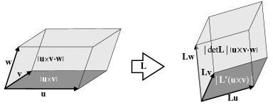
Figure 2.1: Geometrical meaning of the cross and mixed products before (left) and after (right) the application of a tensor $\mathbf{L}$ on the vectors $\mathbf{u},\mathbf{v},\mathbf{w}$.

Because the cross product is antisymmetric and the scalar one is symmetric, it is easy to check that the form

$$\beta(\mathbf{u},\mathbf{v},\mathbf{w})=\mathbf{u}\times\mathbf{v}\cdot\mathbf{w}$$

is a skew trilinear form. Then, Eq. (2.11), we get

$$\mathbf{L}\mathbf{u}\times\mathbf{L}\mathbf{v}\cdot\mathbf{L}\mathbf{w}=\det\mathbf{L}\ \mathbf{u}\times\mathbf{v}\cdot\mathbf{w}.$$ (2.32)

Following the interpretation given above for the absolute value of the mixed product, we can conclude that $|\det\mathbf{L}|$ can be interpreted as a coefficient of volume expansion, cf. again Fig. 2.1. A geometrical interpretation can then be given to the case of a non invertible tensor, i.e. of $\det\mathbf{L}=0$: It crushes a prism into a flat region (the three original vectors become coplanar, i.e. linearly dependent).

The adjugate of $\mathbf{L}$ is the tensor

$$\mathbf{L}^{*}:=(\det\mathbf{L})\mathbf{L}^{-\top}.$$

From Eq. (2.32) we get hence

$$\begin{array}[]{c}\det\mathbf{L}\ \mathbf{u}\times\mathbf{v}\cdot\mathbf{w}=\mathbf{L}\mathbf{u}\times\mathbf{L}\mathbf{v}\cdot\mathbf{L}\mathbf{w}=\mathbf{L}^{\top}(\mathbf{L}\mathbf{u}\times\mathbf{L}\mathbf{v})\cdot\mathbf{w}\ \ \forall\mathbf{w}\Rightarrow\vskip 6.0pt plus 2.0pt minus 2.0pt\\ \mathbf{L}\mathbf{u}\times\mathbf{L}\mathbf{v}=\mathbf{L}^{*}(\mathbf{u}\times\mathbf{v}).\end{array}$$

It is useful, for further development, to calculate the powers of $\mathbf{W}$:

$${\mathbf{W}^{2}}=\mathbf{W}\mathbf{W}=-\mathbf{W}^{\top}(-\mathbf{W}^{\top})=(\mathbf{W}\mathbf{W})^{\top}{=(\mathbf{W}^{2})^{\top}},$$ (2.33)

i.e., $\mathbf{W}^{2}$ is symmetric. Moreover, if we take $\mathbf{w}\in\mathcal{S}$, which is always possible because eigenvectors are determined to within an arbitrary multiplier,

$$\begin{split}{\mathbf{W}^{2}\mathbf{u}}&=\mathbf{W}\mathbf{W}\mathbf{u}=\mathbf{w}\times(\mathbf{w}\times\mathbf{u})=\mathbf{w}\cdot\mathbf{u}\mathbf{w}-\mathbf{w}\cdot\mathbf{w}\mathbf{u}\\ &=-(\mathbf{I}-\mathbf{w}\otimes\mathbf{w})\mathbf{u}\ \Rightarrow\ {\mathbf{W}^{2}{=-(\mathbf{I}-\mathbf{w}\otimes\mathbf{w})}};\end{split}$$ (2.34)

We remark that $\mathbf{W}^{2}\mathbf{u}$ gives the opposite of the projection of any vector $\mathbf{u}\in\mathcal{V}$ onto the direction orthogonal to $\mathbf{w}$, see Exercise 2.

Applying recursively the previous results,

$$\begin{split}&{\mathbf{W}^{3}}=\mathbf{W}\mathbf{W}^{2}=-\mathbf{W}(\mathbf{I}-\mathbf{w}\otimes\mathbf{w})=-\mathbf{W}+(\mathbf{W}\mathbf{w})\otimes\mathbf{w}{=-\mathbf{W}}\\ &{\mathbf{W}^{4}}=\mathbf{W}\mathbf{W}^{3}{=-\mathbf{W}^{2}}\\ &{\mathbf{W}^{5}}=\mathbf{W}\mathbf{W}^{4}{=-\mathbf{W}^{3}}\\ &etc.\end{split}$$ (2.35)

An important property of any couple axial tensor $\mathbf{W}-$axial vector $\mathbf{w}\in\mathcal{S}$ is

$$\mathbf{W}\mathbf{W}=-\frac{1}{2}|\mathbf{W}|^{2}(\mathbf{I}-\mathbf{w}\otimes\mathbf{w}),$$ (2.36)

while Eq. (2.24) can be generalized to any two axial couples $\mathbf{w}_{1},\mathbf{W}_{1}$ and $\mathbf{w}_{2},\mathbf{W}_{2}$ :

$$\mathbf{w}_{1}\cdot\mathbf{w}_{2}=\frac{1}{2}\mathbf{W}_{1}\cdot\mathbf{W}_{2}.$$

The proof of these two last properties is rather easy and left to the reader.

2.10 Orientation of a basis

It is immediate to observe that a basis $\mathcal{B}=\{\mathbf{e}_{1},\mathbf{e}_{2},\mathbf{e}_{3}\}$ can be oriented in two opposite ways: For example, once two unit mutually orthogonal vectors $\mathbf{e}_{1}$ and $\mathbf{e}_{2}$ are chosen, there are two opposite unit vectors perpendicular to both $\mathbf{e}_{1}$ and $\mathbf{e}_{2}$ that can be chosen to form $\mathcal{B}$.

We say that $\mathcal{B}$ is positively oriented or right-handed if

$$\mathbf{e}_{1}\times\mathbf{e}_{2}\cdot\mathbf{e}_{3}=1,$$

while $\mathcal{B}$ is negatively oriented or left-handed if

$$\mathbf{e}_{1}\times\mathbf{e}_{2}\cdot\mathbf{e}_{3}=-1.$$

Schematically, a right-handed basis is represented in Fig. 2.2, where a left-handed basis is represented too with a dashed $\mathbf{e}_{3}$.

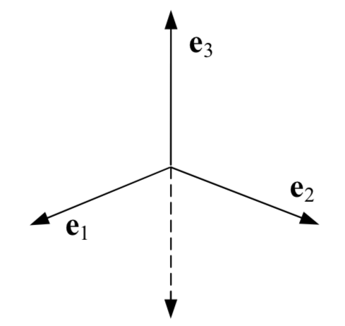
Figure 2.2: Right- and left-handed bases.

With a right-handed basis, by definition, the axial tensors of the three vectors of the basis are

$$\begin{split}&\mathbf{W}_{\mathbf{e}_{1}}=\mathbf{e}_{3}\otimes\mathbf{e}_{2}-\mathbf{e}_{2}\otimes\mathbf{e}_{3},\\ &\mathbf{W}_{\mathbf{e}_{2}}=\mathbf{e}_{1}\otimes\mathbf{e}_{3}-\mathbf{e}_{3}\otimes\mathbf{e}_{1},\\ &\mathbf{W}_{\mathbf{e}_{3}}=\mathbf{e}_{2}\otimes\mathbf{e}_{1}-\mathbf{e}_{1}\otimes\mathbf{e}_{2}.\\ \end{split}$$

2.11 Rotations

In the previous chapter, we have seen that the elements of $\mathcal{V}$ represent translations over $\mathcal{E}$. A rotation, i.e. a rigid rotation of the space, is an operation that transforms any two vectors $\mathbf{u},\mathbf{v}\in\mathcal{V}$ into two other vectors $\hat{\mathbf{u}},\hat{\mathbf{v}}\in\mathcal{V}$ in such a way that

$$u=\hat{u},\ \ v=\hat{v},\ \ \mathbf{u}\cdot\mathbf{v}=\hat{\mathbf{u}}\cdot\hat{\mathbf{v}},$$ (2.37)

i.e., a rotation is a transformation that preserves norms and angles. Because a rotation is a transformation from $\mathcal{V}$ to $\mathcal{V}$, rotations are tensors, so we can write

$$\hat{\mathbf{v}}=\mathbf{R}\mathbf{v},$$

with $\mathbf{R}$ the rotation tensor or simply rotation.

Conditions (2.37) impose some restrictions on $\mathbf{R}$:

$$\hat{\mathbf{u}}\cdot\hat{\mathbf{v}}=\mathbf{R}\mathbf{u}\cdot\mathbf{R}\mathbf{v}=\mathbf{u}\cdot\mathbf{R}^{\top}\mathbf{R}\mathbf{v}=\mathbf{u}\cdot\mathbf{v}\iff\mathbf{R}^{\top}\mathbf{R}=\mathbf{I}=\mathbf{R}\mathbf{R}^{\top}.$$

A tensor that preserves the angles belongs to $Orth(\mathcal{V})$, the subspace of orthogonal tensors; we leave to the reader the proof that actually $Orth(\mathcal{V})$ is actually a subspace of $Lin(\mathcal{V})$. Replacing in the above equation $\mathbf{v}$ with $\mathbf{u}$ shows immediately that an orthogonal tensor also preserves the norms. By the uniqueness of the inverse, we see that

$$\mathbf{R}\in Orth(\mathcal{V})\iff\mathbf{R}^{-1}=\mathbf{R}^{\top}.$$

The above condition is not sufficient to characterize a rotation; in fact, a rotation must transform a right-handed basis into another right-handed basis, i.e. it must preserve the orientation of the space. This means that it must be

$$\hat{\mathbf{e}}_{1}\times\hat{\mathbf{e}}_{2}\cdot\hat{\mathbf{e}}_{3}=\mathbf{R}\mathbf{e}_{1}\times\mathbf{R}\mathbf{e}_{2}\cdot\mathbf{R}\mathbf{e}_{3}=\mathbf{e}_{1}\times\mathbf{e}_{2}\cdot\mathbf{e}_{3}.$$

By Eq. (2.32), we get hence the condition

$$\det\mathbf{R}(\mathbf{e}_{1}\times\mathbf{e}_{2}\cdot\mathbf{e}_{3})=\mathbf{e}_{1}\times\mathbf{e}_{2}\cdot\mathbf{e}_{3}\iff\det\mathbf{R}=1.$$

The tensors of $Orth(\mathcal{V})$ that have a determinant equal to 1 form the subspace of proper rotations or simply rotations, indicated by $Orth(\mathcal{V})^{+}$ or also by $SO(3)$. Only tensors of $Orth(\mathcal{V})^{+}$ represent rigid rotations of $\mathcal{E}$.

Theorem 18.

Each tensor $\mathbf{R}\in Orth(\mathcal{V})$ has the eigenvalue $\pm 1$, with $+1$ for rotations.

Proof.

Let $\mathbf{u}$ be an eigenvector of $\mathbf{R}\in Orth(\mathcal{V})$ corresponding to the eigenvalue $\lambda$. Because $\mathbf{R}$ preserves the norm, we have

$$\mathbf{R}\mathbf{u}\cdot\mathbf{R}\mathbf{u}=\lambda^{2}\mathbf{u}^{2}=\mathbf{u}^{2}\ \rightarrow\ \lambda^{2}=1.$$

We must now prove that there exists at least one real eigenvector $\lambda$. To this end, we consider the characteristic equation

$$f(\lambda)=\lambda^{3}+k_{1}\lambda^{2}+k_{2}\lambda+k_{3}=0,$$

whose coefficients $k_{i}$ are real-valued, because $\mathbf{R}$ has real-valued components. It is immediate to recognize that

$$\lim_{\lambda\rightarrow\pm\infty}f(\lambda)=\pm\infty.$$

So, because $f(\lambda)$ is a real-valued continuous function, actually a polynomial of $\lambda$, there exists at least one $\lambda_{1}\in\mathbb{R}$ such that

$$f(\lambda_{1})=0.$$

In addition, we already know that $\forall\mathbf{R}\in Orth(\mathcal{V}),\det\mathbf{R}=\pm 1$ and that, if $\lambda_{i},i=1,2,3$ are the eigenvalues of $\mathbf{R}$, then $\det\mathbf{R}=\lambda_{1}\lambda_{2}\lambda_{3}$. Hence, the following two are the possible cases:

1. $\lambda_{1}\in\mathbb{R}$ and $\lambda_{2},\lambda_{3}\in\mathbb{C}$, with $\lambda_{3}=\overline{\lambda}_{2}$, the complex conjugate of $\lambda_{2}$;

2. $\lambda_{i}\in\mathbb{R}\ \forall i=1,2,3$.

Let us consider the case of $\mathbf{R}\in Orth(\mathcal{V})^{+}$, i.e. a (proper) rotation $\rightarrow\det\mathbf{R}=1$. Then, in the first case above,

$$\det\mathbf{R}=\lambda_{1}\lambda_{2}\overline{\lambda}_{2}=\lambda_{1}[\Re^{2}(\lambda_{2})+\Im^{2}(\lambda_{2})].$$

But

$$\Re^{2}(\lambda_{2})+\Im^{2}(\lambda_{2})=1$$

because it is the square of the modulus of the complex eigenvalue $\lambda_{2}$. So in this case

$$\det\mathbf{R}=1\iff\lambda_{1}=1.$$

In the second case, $\lambda_{i}\in\mathbb{R}\ \forall i=1,2,3$, either $\lambda_{1}>0,\lambda_{2},\lambda_{3}<0$, or all of them are positive. Because the modulus of each eigenvalue must be equal to 1, either $\lambda_{1}=1$ or $\lambda_{i}=1\ \forall i=1,2,3$ (in this case, $\mathbf{R}=\mathbf{I}$).

Following the same steps, one can easily show that $\forall\mathbf{S}\in Orth(\mathcal{V})$ with $\det\mathbf{S}=-1$, there exists at least one real eigenvalue $\lambda_{1}=-1$. ∎

Generally, a rotation tensor rotates the basis $\mathcal{B}=\{\mathbf{e}_{1},\mathbf{e}_{2},\mathbf{e}_{3}\}$ into the basis $\hat{\mathcal{B}}=\{\hat{\mathbf{e}}_{1},\hat{\mathbf{e}}_{2},\hat{\mathbf{e}}_{3}\}$:

$$\mathbf{R}\mathbf{e}_{i}=\hat{\mathbf{e}}_{i}\ \ \forall i=1,2,3\ \Rightarrow\ {R_{ij}=\mathbf{e}_{i}\cdot\mathbf{R}\mathbf{e}_{j}=\mathbf{e}_{i}\cdot\hat{\mathbf{e}}_{j}}.$$ (2.38)

This result actually means that the $j$th column of $\mathbf{R}$ is formed by the components in the basis $\mathcal{B}$ of the vector $\hat{\mathbf{e}}_{j}$ of $\hat{\mathcal{B}}$. Because the two bases are orthonormal, such components are the director cosines of the axes of $\hat{\mathcal{B}}$ with respect to $\mathcal{B}$.

Geometrically, any rotation is characterized by an axis of rotation ${\mathbf{w}},|\mathbf{w}|=1$, and by an amplitude $\varphi$, i.e. the angle through which the space is rotated about $\mathbf{w}$. By definition, $\mathbf{w}$ is the (only) vector that is left unchanged by $\mathbf{R}$, i.e.

$$\mathbf{R}\mathbf{w}=\mathbf{w},$$

or, in other words, it is the eigenvector corresponding to the eigenvalue $+1$.

The question is then: How can a rotation tensor $\mathbf{R}$ be expressed by means of its geometrical parameters, $\mathbf{w}$ and $\varphi$? To this end we have a fundamental theorem:

Theorem 19.

(Euler’s rotation representation theorem). $\forall\mathbf{R}\in Orth(\mathcal{V})^{+}$,

$${\mathbf{R}=\mathbf{I}+\sin\varphi\mathbf{W}+(1-\cos\varphi)\mathbf{W}^{2}}$$ (2.39)

with $\varphi$ the rotation’s amplitude and $\mathbf{W}$ the axial tensor of the rotation axis $\mathbf{w}$.

Proof.

We observe preliminarily that

$${\mathbf{R}\mathbf{w}}=\mathbf{I}\mathbf{w}+\sin\varphi\mathbf{W}\mathbf{w}+(1-\cos\varphi)\mathbf{W}\mathbf{W}\mathbf{w}=\mathbf{I}\mathbf{w}={\mathbf{w}}$$ (2.40)

i.e. that Eq. (2.39) actually defines a transformation that leaves unchanged the axis $\mathbf{w}$, like a rotation about $\mathbf{w}$ must do, and that $+1$ is an eigenvalue of $\mathbf{R}$.

We need now to prove that Eq. (2.39) actually represents a rotation tensor, i.e. we must prove that

$$\mathbf{R}\mathbf{R}^{\top}=\mathbf{I},\ \ \det\mathbf{R}=1.$$

Through Eq. (2.35) we get

$$\begin{split}{\mathbf{R}\mathbf{R}^{\top}}&=(\mathbf{I}+\sin\varphi\mathbf{W}+(1-\cos\varphi)\mathbf{W}^{2})(\mathbf{I}+\sin\varphi\mathbf{W}+(1-\cos\varphi)\mathbf{W}^{2})^{\top}\\ &=(\mathbf{I}+\sin\varphi\mathbf{W}+(1-\cos\varphi)\mathbf{W}^{2})(\mathbf{I}-\sin\varphi\mathbf{W}+(1-\cos\varphi)\mathbf{W}^{2})\\ &=\mathbf{I}+2(1-\cos\varphi)\mathbf{W}^{2}-\sin^{2}\varphi\mathbf{W}^{2}+(1-\cos\varphi)^{2}\mathbf{W}^{4}\\ &=\mathbf{I}+2(1-\cos\varphi)\mathbf{W}^{2}-\sin^{2}\varphi\mathbf{W}^{2}-(1-\cos\varphi)^{2}\mathbf{W}^{2}{=\mathbf{I}}.\end{split}$$

Then, through Eq. (2.34), we obtain

$$\begin{split}{\mathbf{R}}&=\mathbf{I}+\sin\varphi\mathbf{W}+(1-\cos\varphi)\mathbf{W}^{2}\\ &=\mathbf{I}+\sin\varphi\mathbf{W}-(1-\cos\varphi)(\mathbf{I}-\mathbf{w}\otimes\mathbf{w})\\ &{=\cos\varphi\mathbf{I}+\sin\varphi\mathbf{W}+(1-\cos\varphi)\mathbf{w}\otimes\mathbf{w}}.\end{split}$$ (2.41)

To go on, we need to express $\mathbf{W}$ and $\mathbf{w}\otimes\mathbf{w}$; if $\mathbf{w}=(w_{1},w_{2},w_{3})$, then by Eq. (2.23) we have

$${\mathbf{W}=\left[\begin{array}[]{ccc}0&-w_{3}&w_{2}\\ w_{3}&0&-w_{1}\\ -w_{2}&w_{1}&0\end{array}\right]}$$

and by Eq. (2.2),

$$\mathbf{w}\otimes\mathbf{w}=\left[\begin{array}[]{ccc}w_{1}^{2}&w_{1}w_{2}&w_{1}w_{3}\\ w_{1}w_{2}&w_{2}^{2}&w_{2}w_{3}\\ w_{1}w_{3}&w_{2}w_{3}&w_{3}^{2}\end{array}\right],$$

which on injecting into Eq. (2.41) gives

$$\mathbf{R}=\left[\begin{array}[]{ccc}\cos\varphi+(1-\cos\varphi)w_{1}^{2}&-w_{3}\sin\varphi+w_{1}w_{2}(1-\cos\varphi)&w_{2}\sin\varphi+w_{1}w_{3}(1-\cos\varphi)\\ w_{3}\sin\varphi+w_{1}w_{2}(1-\cos\varphi)&\cos\varphi+(1-\cos\varphi)w_{2}^{2}&-w_{1}\sin\varphi+w_{2}w_{3}(1-\cos\varphi)\\ -w_{2}\sin\varphi+w_{1}w_{3}(1-\cos\varphi)&w_{1}\sin\varphi+w_{2}w_{3}(1-\cos\varphi)&\cos\varphi+(1-\cos\varphi)w_{3}^{2}\end{array}\right].$$ (2.42)

This formula gives $\mathbf{R}$ as a function exclusively of $\mathbf{w}$ and $\varphi$, the geometrical elements of the rotation. Then

$$\det\mathbf{R}=(w^{2}+(1-w^{2})\cos\varphi)(\cos^{2}\varphi+w^{2}\sin^{2}\varphi)$$

and because $w=1,{\det\mathbf{R}=1}$, which proves that Eq. (2.39) actually represents a rotation.

We eventually need to prove that Eq. (2.39) represents the rotation about $\mathbf{w}$ of amplitude $\varphi$. To this end, we choose an orthonormal basis $\mathcal{B}=\{\mathbf{e}_{1},\mathbf{e}_{2},\mathbf{e}_{3}\}$ of $\mathcal{V}$ such that $\mathbf{w}=\mathbf{e}_{3}$, i.e. we analyze the particular case of a rotation of amplitude $\varphi$ about $\mathbf{e}_{3}$. This is always possible thanks to the arbitrariness of the basis of $\mathcal{V}$. In such a case, Eq. (2.38) gives

$$\mathbf{R}=\left[\begin{array}[]{ccc}\cos\varphi&-\sin\varphi&0\\ \sin\varphi&\cos\varphi&0\\ 0&0&1\end{array}\right].$$ (2.43)

Moreover,

$$\begin{split}&{\mathbf{W}=\left[\begin{array}[]{ccc}0&-1&0\\ 1&0&0\\ 0&0&0\end{array}\right],\ \ \ \mathbf{w}\otimes\mathbf{w}=\left[\begin{array}[]{ccc}0&0&0\\ 0&0&0\\ 0&0&1\end{array}\right]},\\ &{\mathbf{W}^{2}=-(\mathbf{I}-\mathbf{w}\otimes\mathbf{w})=\left[\begin{array}[]{ccc}-1&0&0\\ 0&-1&0\\ 0&0&0\end{array}\right]}.\end{split}$$

Hence

$$\begin{split}&{\mathbf{I}+\sin\varphi\mathbf{W}+(1-\cos\varphi)\mathbf{W}^{2}}=\left[\begin{array}[]{ccc}1&0&0\\ 0&1&0\\ 0&0&1\end{array}\right]+\sin\varphi\left[\begin{array}[]{ccc}0&-1&0\\ 1&0&0\\ 0&0&0\end{array}\right]+\\ &+(1-\cos\varphi)\left[\begin{array}[]{ccc}-1&0&0\\ 0&-1&0\\ 0&0&0\end{array}\right]=\left[\begin{array}[]{ccc}\cos\varphi&-\sin\varphi&0\\ \sin\varphi&\cos\varphi&0\\ 0&0&1\end{array}\right]{=\mathbf{R}}.\end{split}$$ (2.44)

∎

Equation (2.39) gives another result: To obtain the inverse of $\mathbf{R}$ it is sufficient to change the sign of $\varphi$. In fact, because $\mathbf{W}\in Skw(\mathcal{V})$ and through Eq. (2.33)

$$\begin{split}\mathbf{R}^{-1}=\mathbf{R}^{\top}&=(\mathbf{I}+\sin\varphi\mathbf{W}+(1-\cos\varphi)\mathbf{W}^{2})^{\top}=\mathbf{I}+\sin\varphi\mathbf{W}^{\top}+(1-\cos\varphi)(\mathbf{W}^{2})^{\top}\\ &=\mathbf{I}-\sin\varphi\mathbf{W}+(1-\cos\varphi)\mathbf{W}^{2}=\mathbf{I}+\sin(-\varphi)\mathbf{W}+(1-\cos(-\varphi))\mathbf{W}^{2}.\end{split}$$

The knowledge of the inverse of a rotation also allows us to perform the operation of change of basis, i.e. to determine the components of a vector or of a tensor in a basis $\hat{\mathcal{B}}=\{\hat{\mathbf{e}}_{1},\hat{\mathbf{e}}_{2},\hat{\mathbf{e}}_{3}\}$ rotated with respect to an original basis $\mathcal{B}=\{\mathbf{e}_{1},\mathbf{e}_{2},\mathbf{e}_{3}\}$ by a rotation $\mathbf{R}$ (in the following equations, the symbol $\ \hat{}\$ indicates a quantity specified in the basis $\hat{\mathcal{B}}$). Considering that

$$\mathbf{e}_{i}=\mathbf{R}^{-1}\hat{\mathbf{e}}_{i}=\mathbf{R}^{\top}\hat{\mathbf{e}}_{i}=R_{hk}^{\top}(\hat{\mathbf{e}}_{h}\otimes\hat{\mathbf{e}}_{k})\hat{\mathbf{e}}_{i}=R^{\top}_{hk}\delta_{ki}\hat{\mathbf{e}}_{h}$$

we get, for a vector $\mathbf{u}$,

$$\mathbf{u}=u_{i}\mathbf{e}_{i}=R^{\top}_{ki}u_{i}\hat{\mathbf{e}}_{k}$$

i.e.

$$\hat{u}_{k}=R^{\top}_{ki}u_{i}\ \rightarrow\ \hat{\mathbf{u}}=\mathbf{R}^{\top}\mathbf{u}.$$

We remark that, because $\mathbf{R}^{\top}=\mathbf{R}^{-1}$, the operation of change of basis is just the opposite of the rotation of the space (and actually, we have seen that it is sufficient to take the opposite of $\varphi$ in Eq. (2.39) to get $\mathbf{R}^{-1}$).

For a second-rank tensor $\mathbf{L}$ we get

$$\mathbf{L}=L_{ij}\mathbf{e}_{i}\otimes\mathbf{e}_{j}=L_{ij}R^{\top}_{mi}\hat{\mathbf{e}}_{m}\otimes R^{\top}_{nj}\hat{\mathbf{e}}_{n}=R^{\top}_{mi}R^{\top}_{nj}L_{ij}\hat{\mathbf{e}}_{m}\otimes\hat{\mathbf{e}}_{n},$$

i.e.

$$\hat{L}_{mn}=R^{\top}_{mi}R^{\top}_{nj}L_{ij}\ =R^{\top}_{mi}L_{ij}R_{jn}\ \rightarrow\ \hat{\mathbf{L}}=\mathbf{R}^{\top}\mathbf{L}\mathbf{R}.$$

We remark something that is typical of tensors: the components of a $r$-rank tensor in a rotated basis $\hat{\mathcal{B}}$ depend upon the $r$th powers of the directors cosines of the axes of $\hat{\mathcal{B}}$, i.e. on the $r$th powers of the components $R_{ij}$ of $\mathbf{R}$.

If a rotation tensor is known through its Cartesian components in a given basis $\mathcal{B}$, it is easy to calculate its geometrical elements: The rotation axis $\mathbf{w}$ is the eigenvector of $\mathbf{R}$ corresponding to the eigenvalue 1, so it is found solving the equation

$$\mathbf{R}\mathbf{w}=\mathbf{w}$$

and then normalizing it, while the rotation amplitude $\varphi$ can be found using (2.39) along with (2.34): Because the trace of a tensor is an invariant, we get

$$\mathrm{tr}\mathbf{R}=3+(1-\cos\varphi)\mathrm{tr}(-\mathbf{I}+\mathbf{w}\otimes\mathbf{w})=1+2\cos\varphi\ \rightarrow\ \varphi=\arccos\frac{\mathrm{tr}\mathbf{R}-1}{2}.$$

It is interesting to consider the geometrical meaning of Eq. (2.39). For this purpose, we apply Eq. (2.39) to a vector $\mathbf{u}$, see Fig. 2.3,

$$\begin{split}\mathbf{R}\mathbf{u}&=(\mathbf{I}+\sin\varphi\mathbf{W}+(1-\cos\varphi)\mathbf{W}^{2})\mathbf{u}\\ &=\mathbf{u}+\sin\varphi\mathbf{w}\times\mathbf{u}+(1-\cos\varphi)\mathbf{w}\times(\mathbf{w}\times\mathbf{u})\end{split}$$

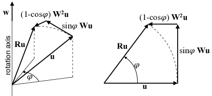
Figure 2.3: Rotation of a vector.

The rotated vector $\mathbf{R}\mathbf{u}$ is the sum of three vectors; in particular, $\sin\varphi\mathbf{W}\mathbf{u}$ is always orthogonal to $\mathbf{u}$, $\mathbf{w}$ and $(1-\cos\varphi)\mathbf{W}^{2}\mathbf{u}$. If $\mathbf{u}\cdot\mathbf{w}=0$, then $(1-\cos\varphi)\mathbf{W}^{2}\mathbf{u}$ is also parallel to $\mathbf{u}$, see the sketch on the right in Fig. 2.3.

Let us consider now a composition of rotations. In particular, let us imagine that a vector $\mathbf{u}$ is rotated first by $\mathbf{R}_{1}$ around $\mathbf{w}_{1}$ through $\varphi_{1}$, then by $\mathbf{R}_{2}$ around $\mathbf{w}_{2}$ through $\varphi_{2}$. So, first, the vector $\mathbf{u}$ becomes the vector

$$\mathbf{u}_{1}=\mathbf{R}_{1}\mathbf{u}.$$

Then, the vector $\mathbf{u}_{1}$ is rotated about $\mathbf{w}_{2}$ through $\varphi_{2}$ to become

$$\mathbf{u}_{12}=\mathbf{R}_{2}\mathbf{u}_{1}=\mathbf{R}_{2}\mathbf{R}_{1}\mathbf{u}.$$

Let us now suppose that we change the order of the rotations: $\mathbf{R}_{2}$ first and then $\mathbf{R}_{1}$. The final result will be the vector

$$\mathbf{u}_{21}=\mathbf{R}_{1}\mathbf{R}_{2}\mathbf{u}.$$ (2.45)

Because the tensor product is not symmetric (i.e., it has not the commutativity property), generally

$${\mathbf{u}_{12}\neq\mathbf{u}_{21}}.$$

In other words, the order of the rotations matters: Changing the order of the rotations leads to a different final result. An example is shown in Fig. 2.4.

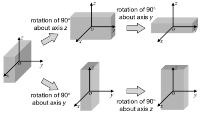
Figure 2.4: Non-commutativity of the rotations.

This is a fundamental difference between rotations and displacements, that commute, see Fig. 1.2, because the composition of displacements is ruled by the sum of vectors:

$$\mathbf{w}=\mathbf{u}+\mathbf{v}=\mathbf{v}+\mathbf{u}$$ (2.46)

This difference, which is a major point in physics, comes from the difference in the operators: vectors for the displacements and tensors for the rotations.

Any rotation can be specified by the knowledge of three parameters. This can be easily seen from Eq. (2.39): the parameters are the three components of $\mathbf{w}$, that are not independent because

$$w=|\mathbf{w}|=\sqrt{w_{1}^{2}+w_{2}^{2}+w_{3}^{2}}=1$$

and by the amplitude angle $\varphi$. The choice of the parameters by which to express a rotation is not unique. Besides the use of the Cartesian components of $\mathbf{w}$ and $\varphi$, cf. Eq. (2.42), other choices are possible, let us see three of them:

1. Physical angles: The rotation axis $\mathbf{w}$ is given through its spherical coordinates $\psi$, the longitude, $0\leq\psi<2\pi$, and $\theta$, the colatitude, $0\leq\theta\leq\pi$, see Fig. 2.5, the third parameter being the rotation amplitude $\varphi$.

   

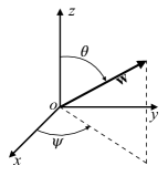
   Figure 2.5: Physical angles.

   Then

   $$\mathbf{w}=(\sin\theta\cos\psi,\sin\theta\sin\psi,\cos\theta)\ \rightarrow\ \theta=\arccos w_{3},\ \psi=\arctan\frac{w_{2}}{w_{1}},$$

   and, Eq. (2.42),

   $$\mathbf{R}=\left[\begin{array}[]{ccc}c\psi^{2}s\theta^{2}+c\varphi(c\theta^{2}+s\psi^{2}s\theta^{2})&s\psi c\psi s\theta^{2}(1-c\varphi)-c\theta s\varphi&c\psi s\theta c\theta(1-c\varphi)+s\psi s\theta s\varphi\\ s\psi c\psi s\theta^{2}(1-c\varphi)+c\theta s\varphi&s\psi^{2}s\theta^{2}+c\varphi(c\theta^{2}+c\psi^{2}s\theta^{2})&s\psi s\theta c\theta(1-c\varphi)-c\psi s\theta s\varphi\\ c\psi s\theta c\theta(1-c\varphi)-s\psi s\theta s\varphi&s\psi s\theta c\theta(1-c\varphi)+c\psi s\theta s\varphi&c\theta^{2}+c\varphi(c\psi^{2}s\theta^{2}+s\psi^{2}s\theta^{2})\end{array}\right],$$

   where $c\psi=\cos\psi,s\psi=\sin\psi,c\theta=\cos\theta,s\theta=\sin\theta,c\varphi=\cos\varphi$ and $s\varphi=\sin\varphi$. We remark that all the components of $\mathbf{R}$ so expressed depend upon the first powers of the circular functions of $\varphi$. Hence, for what is said above, with this representation of the rotations, the components of a rotated $r$-rank tensor depend upon the $r$th power of the circular functions of $\varphi$, i.e. of the physical rotation, but not of $\psi$ nor of $\theta$.

2. Euler’s angles: In this case, the three parameters are the amplitude of three particular rotations into which the rotation is decomposed. Such parameters are the angles $\psi$, the precession, $\theta$, the nutation, and $\varphi$, the proper rotation, see Fig. 2.6

   

   Figure 2.6: Euler’s angles.

   These three rotations are represented in Fig. 2.7. The first one, of amplitude $\psi$, is made about $z$ to carry the axis $x$ onto the knots line $x_{N}$, the line perpendicular to both the axes $z$ and $\hat{z}$, and $y$ onto $\overline{y}$; by Eq. (2.38), in the frame $\{x,y,z\}$ it is

   $$\mathbf{R}_{\psi}=\left[\begin{array}[]{ccc}\cos\psi&-\sin\psi&0\\ \sin\psi&\cos\psi&0\\ 0&0&1\end{array}\right].$$

   The second one, of amplitude $\theta$, is made about $x_{N}$ to carry $z$ onto $\hat{z}$; in the frame $\{x_{N},\overline{y},z\}$, it is

   $$\mathbf{R}_{\theta}=\left[\begin{array}[]{ccc}1&0&0\\ 0&\cos\theta&-\sin\theta\\ 0&\sin\theta&\cos\theta\end{array}\right],$$

   while in the frame $\{x,y,z\}$,

   $$\mathbf{R}_{\theta}^{o}=(\mathbf{R}_{\psi}^{-1})^{\top}\mathbf{R}_{\theta}\mathbf{R}_{\psi}^{-1}=\mathbf{R}_{\psi}\mathbf{R}_{\theta}\mathbf{R}_{\psi}^{\top}.$$

   

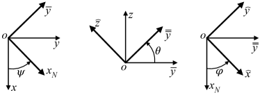
   Figure 2.7: Euler’s rotations, as seen from the respective axes of rotation.

   The last rotation, of amplitude $\varphi$, is made about $\hat{z}$ to carry $x_{N}$ onto $\hat{x}$ and $\overline{\overline{y}}$ onto $\hat{y}$; in the frame $\{x_{N},\overline{\overline{y}},\hat{z}\}$, it is

   $$\mathbf{R}_{\varphi}=\left[\begin{array}[]{ccc}\cos\varphi&-\sin\varphi&0\\ \sin\varphi&\cos\varphi&0\\ 0&0&1\end{array}\right],$$

   while in $\{x,y,z\}$,

   $$\mathbf{R}_{\varphi}^{o}=(\mathbf{R}_{\psi}^{-1})^{\top}(\mathbf{R}_{\theta}^{-1})^{\top}\mathbf{R}_{\varphi}\mathbf{R}_{\theta}^{-1}\mathbf{R}_{\psi}^{-1}=\mathbf{R}_{\psi}\mathbf{R}_{\theta}\mathbf{R}_{\varphi}\mathbf{R}_{\theta}^{\top}\mathbf{R}_{\psi}^{\top}.$$

   Any vector $\mathbf{u}$ is transformed, by the global rotation, into the vector

   $$\hat{\mathbf{u}}=\mathbf{R}\mathbf{u}.$$

   But we can also write

   $$\hat{\mathbf{u}}=\mathbf{R}_{\varphi}^{o}\overline{\overline{\mathbf{u}}},$$

   where $\overline{\overline{\mathbf{u}}}$ is the vector transformed by the rotation $\mathbf{R}_{\theta}^{o}$,

   $$\overline{\overline{\mathbf{u}}}=\mathbf{R}_{\theta}^{o}\overline{\mathbf{u}},$$

   and $\overline{\mathbf{u}}$ is the vector transformed by the rotation $\mathbf{R}_{\psi}$:

   $$\overline{\mathbf{u}}=\mathbf{R}_{\psi}\mathbf{u}.$$

   Finally,

   $$\hat{\mathbf{u}}=\mathbf{R}\mathbf{u}=\mathbf{R}_{\varphi}^{o}\mathbf{R}_{\theta}^{o}\mathbf{R}_{\psi}\mathbf{u}\ \rightarrow\ \mathbf{R}=\mathbf{R}_{\varphi}^{o}\mathbf{R}_{\theta}^{o}\mathbf{R}_{\psi},$$

   i.e. the global rotation tensor is obtained composing, in the opposite order of execution of the rotations, the three tensors all expressed in the original basis. However,

   $$\mathbf{R}=\mathbf{R}_{\varphi}^{o}\mathbf{R}_{\theta}^{o}\mathbf{R}_{\psi}=\mathbf{R}_{\psi}\mathbf{R}_{\theta}\mathbf{R}_{\varphi}\mathbf{R}_{\theta}^{\top}\mathbf{R}_{\psi}^{\top}\mathbf{R}_{\psi}\mathbf{R}_{\theta}\mathbf{R}_{\psi}^{\top}\mathbf{R}_{\psi}=\mathbf{R}_{\psi}\mathbf{R}_{\theta}\mathbf{R}_{\varphi},$$

   i.e., the global rotation tensor is also equal to the composition of the three rotations, in the order of execution, if the three rotations are expressed in their own particular bases. This result is general, not bounded to the Euler’s rotations nor to three rotations.

   Performing the tensor multiplications, we get

   $$\mathbf{R}=\left[\begin{array}[]{ccc}\cos\psi\cos\varphi-\sin\psi\sin\varphi\cos\theta&-\cos\psi\sin\varphi-\sin\psi\cos\varphi\cos\theta&\sin\psi\sin\theta\\ \sin\psi\cos\varphi+\cos\psi\sin\varphi\cos\theta&-\sin\psi\sin\varphi+\cos\psi\cos\varphi\cos\theta&-\cos\psi\sin\theta\\ \sin\varphi\sin\theta&\cos\varphi\sin\theta&\cos\theta\end{array}\right].$$

   The components of a vector $\mathbf{u}$ in the basis $\hat{\mathcal{B}}$ are then given by

   $$\hat{\mathbf{u}}=\mathbf{R}^{\top}\mathbf{u}=\mathbf{R}_{\varphi}^{\top}\mathbf{R}_{\theta}^{\top}\mathbf{R}_{\psi}^{\top}\mathbf{u},$$

   and those of a second-rank tensor

   $$\hat{\mathbf{L}}=\mathbf{R}^{\top}\mathbf{L}\mathbf{R}=\mathbf{R}_{\varphi}^{\top}\mathbf{R}_{\theta}^{\top}\mathbf{R}_{\psi}^{\top}\mathbf{L}\mathbf{R}_{\psi}\mathbf{R}_{\theta}\mathbf{R}_{\varphi}.$$

3. Coordinate angles: In this case, the rotation $\mathbf{R}$ is decomposed into three successive rotations $\alpha,\beta,\gamma$, respectively about the axes $x$, $y$ and $z$ of each rotation, i.e.

   $$\mathbf{R}=\mathbf{R}_{\alpha}\mathbf{R}_{\beta}\mathbf{R}_{\gamma}$$

   with

   $$\mathbf{R}_{\alpha}=\left[\begin{array}[]{ccc}1&0&0\\ 0&\cos\alpha&-\sin\alpha\\ 0&\sin\alpha&\cos\alpha\end{array}\right],\mathbf{R}_{\beta}=\left[\begin{array}[]{ccc}\cos\beta&0&-\sin\beta\\ 0&1&0\\ \sin\beta&0&\cos\beta\end{array}\right],\mathbf{R}_{\gamma}=\left[\begin{array}[]{ccc}\cos\gamma&-\sin\gamma&0\\ \sin\gamma&\cos\gamma&0\\ 0&0&1\end{array}\right],$$

   so finally

   $$\mathbf{R}=\left[\begin{array}[]{ccc}\cos\beta\cos\gamma&-\cos\beta\sin\gamma&-\sin\beta\\ \cos\alpha\sin\gamma-\sin\alpha\sin\beta\cos\gamma&\cos\alpha\cos\gamma+\sin\alpha\sin\beta\sin\gamma&-\sin\alpha\cos\beta\\ \sin\alpha\sin\gamma+\cos\alpha\sin\beta\cos\gamma&\sin\alpha\cos\gamma-\cos\alpha\sin\beta\sin\gamma&\cos\alpha\cos\beta\end{array}\right].$$

Let us now consider the case of small rotations, i.e. $|\varphi|\rightarrow 0$. In such a case,

$$\sin\varphi\simeq\varphi,\ \ 1-\cos\varphi\simeq 0$$

so that the Euler’s theorem, Eq. (2.39), becomes

$$\mathbf{R}\simeq\mathbf{I}+\varphi\mathbf{W},$$

i.e. in the small rotations approximation, any vector $\mathbf{u}$ is transformed into

$$\mathbf{R}\mathbf{u}\simeq(\mathbf{I}+\varphi\mathbf{W})\mathbf{u}=\mathbf{u}+\varphi\mathbf{w}\times\mathbf{u},$$ (2.47)

i.e. by a skew tensor and not by a rotation tensor. The term $(1-\cos\varphi)\mathbf{W}^{2}\mathbf{u}$ has disappeared, as it is a higher-order infinitesimal quantity, and the term $\varphi\mathbf{w}\times\mathbf{u}$ is orthogonal to $\mathbf{u}$. Because $\varphi\rightarrow 0$, the arc is approximated by its tangent, the vector $\varphi\mathbf{w}\times\mathbf{u}$, see Fig. 2.8.

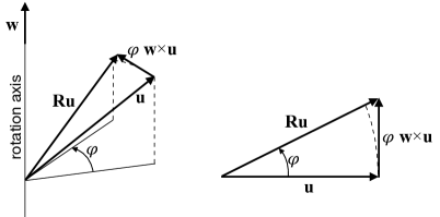
Figure 2.8: Small rotations.

Applying to Eq. (2.47) the procedure already seen for the composition of finite amplitude rotations, we get

$$\begin{split}&\mathbf{u}_{1}\ =\mathbf{R}_{1}\mathbf{u}=(\mathbf{I}+\varphi_{1}\mathbf{W}_{1})\mathbf{u}=\mathbf{u}+\varphi_{1}\mathbf{w}_{1}\times\mathbf{u},\\ &\mathbf{u}_{21}=\mathbf{R}_{2}\mathbf{u}_{1}=(\mathbf{I}+\varphi_{2}\mathbf{W}_{2})\mathbf{u}_{1}=\mathbf{u}_{1}+\varphi_{2}\mathbf{w}_{2}\times\mathbf{u}_{1}\\ &\hskip 15.649pt=\mathbf{u}+\varphi_{1}\mathbf{w}_{1}\times\mathbf{u}+\varphi_{2}\mathbf{w}_{2}\times\mathbf{u}\\ &\hskip 28.45274pt+\varphi_{1}\varphi_{2}\mathbf{w}_{2}\times(\mathbf{w}_{1}\times\mathbf{u}).\end{split}$$

If the order of the rotations is changed, the last term becomes $\varphi_{1}\varphi_{2}\mathbf{w}_{1}\times(\mathbf{w}_{2}\times\mathbf{u})$, which is, in general, different from $\varphi_{1}\varphi_{2}\mathbf{w}_{2}\times(\mathbf{w}_{1}\times\mathbf{u})$: Strictly speaking, also small rotations do not commute. However, for small rotations, $\varphi_{1}\varphi_{2}$ is negligible with respect to $\varphi_{1}$ and $\varphi_{2}$: In this approximation, small rotations commute. We remark that the approximation (2.47) gives, for the displacements, a law that is quite similar to that of the velocities of the points of a rigid body:

$$\mathbf{v}=\mathbf{v}_{0}+\boldsymbol{\omega}\times(p-o)$$

This is quite natural, because

$$\omega=\frac{d\varphi}{dt},$$

i.e. a small amplitude rotation can be seen as the rotation made with finite angular velocity $\boldsymbol{\omega}$ in a small time interval $dt$.

2.12 Reflexions

Let us consider now tensors $\mathbf{S}\in Orth(\mathcal{V})$ that are not a rotation, i.e. such that $\det\mathbf{S}=-1$. Let us call $\mathbf{S}$ an improper rotation. A particular improper rotation, whose all eigenvalues are equal to -1, is the inversion or reflexion tensor:

$$\mathbf{S}_{I}=-\mathbf{I}.$$

The effect of $\mathbf{S}_{I}$ is to transform any basis $\mathcal{B}$ into the basis $-\mathcal{B}$, i.e. with all the basis vectors changed in orientation (or, equivalently, to change the sign of all the components of a vector). In other words, $\mathbf{S}_{I}$ changes the orientation of the space. This is also the effect of any other improper rotation $\mathbf{S}$, that can be decomposed into a proper rotation $\mathbf{R}$ followed by the reflexion $\mathbf{S}_{I}$:

$$\mathbf{S}=\mathbf{S}_{I}\mathbf{R}.$$ (2.48)

Let $\mathbf{n}\in\mathcal{S}$; then

$$\mathbf{S}_{R}=\mathbf{I}-2\mathbf{n}\otimes\mathbf{n}$$ (2.49)

is the tensor that operates the transformation of symmetry with respect to a plane orthogonal to $\mathbf{n}$. In fact

$$\mathbf{S}_{R}\mathbf{n}=-\mathbf{n},\ \ \mathbf{S}_{R}\mathbf{m}=\mathbf{m}\ \ \forall\mathbf{m}\in\mathcal{V}|\ \mathbf{m}\cdot\mathbf{n}=0.$$

$\mathbf{S}_{R}$ is an improper rotation; in fact, by Eq. (2.4),

$$\begin{split}(\mathbf{I}-2\mathbf{n}\otimes\mathbf{n})(\mathbf{I}-2\mathbf{n}\otimes\mathbf{n})^{\top}&=(\mathbf{I}-2\mathbf{n}\otimes\mathbf{n})(\mathbf{I}-2\mathbf{n}\otimes\mathbf{n})\\ &=\mathbf{I}-2\mathbf{n}\otimes\mathbf{n}-2\mathbf{n}\otimes\mathbf{n}+4(\mathbf{n}\otimes\mathbf{n})(\mathbf{n}\otimes\mathbf{n})=\mathbf{I},\end{split}$$

while by the same definition of trace and through Eqs. (2.13) and (2.17),

$$\det(\mathbf{I}-2\mathbf{n}\otimes\mathbf{n})=1-2\mathrm{tr}(\mathbf{n}\otimes\mathbf{n})+4\frac{\mathrm{tr}^{2}(\mathbf{n}\otimes\mathbf{n})-\mathrm{tr}(\mathbf{n}\otimes\mathbf{n})(\mathbf{n}\otimes\mathbf{n})}{2}-8\det(\mathbf{n}\otimes\mathbf{n})=-1.$$

Let $\mathbf{S}=\mathbf{S}_{I}\mathbf{R}$ be an improper rotation. Then

$$\begin{split}(\mathbf{S}\mathbf{u})\times(\mathbf{S}\mathbf{v})&=(\mathbf{S}_{I}\mathbf{R}\mathbf{u})\times(\mathbf{S}_{I}\mathbf{R}\mathbf{v})=\det(\mathbf{S}_{I}\mathbf{R})\left[(\mathbf{S}_{I}\mathbf{R})^{-1}\right]^{\top}(\mathbf{u}\times\mathbf{v})\\ &=\det\mathbf{S}_{I}\det\mathbf{R}(\mathbf{R}^{-1}\mathbf{S}_{I}^{-1})^{\top}(\mathbf{u}\times\mathbf{v})=-(-\mathbf{R}^{-1}\mathbf{I})^{\top}(\mathbf{u}\times\mathbf{v})=\mathbf{R}(\mathbf{u}\times\mathbf{v}).\end{split}$$

The transformation by $\mathbf{S}$ of any vector $\mathbf{u}$ gives

$$\mathbf{S}\mathbf{u}=\mathbf{S}_{I}\mathbf{R}\mathbf{u}=-\mathbf{R}\mathbf{u},$$

i.e. it changes the orientation of the rotated vector; this is not the case when the same improper rotations transforms the vectors of a cross product: The rotated vector, result of the cross product, does not change of orientation, i.e. the cross product is insensitive to a reflexion. That is why, strictly speaking, the result of a cross product is not a vector, but a pseudo-vector: It behaves like vectors apart for the reflexions. For the same reason, a scalar result of a mixed product (scalar plus cross product of three vectors) is called a pseudo-scalar because in this case, the scalar result of the mixed product changes of sign under a reflexion, which can be checked easily.

2.13 Polar decomposition

Theorem 20.

(Square root theorem). Consider $\mathbf{L}\in Sym(\mathcal{V})$ and positive definite. Then, there exists a unique tensor $\mathbf{U}\in Sym(\mathcal{V})$ and positive definite such that

$$\mathbf{L}=\mathbf{U}^{2}.$$

Proof.

Existence: Consider $\mathbf{L},\mathbf{U},\mathbf{V}\in Sym(\mathcal{V})$ and positive definite, and

$$\mathbf{L}=\omega_{i}\mathbf{e}_{i}\otimes\mathbf{e}_{i}$$

a spectral decomposition of $\mathbf{L}$, $\omega_{i}>0\ \forall i$. Define $\mathbf{U}$ as

$$\mathbf{U}=\sqrt{\omega_{i}}\mathbf{e}_{i}\otimes\mathbf{e}_{i};$$

then, by Eq. (2.4)₁, we get

$$\mathbf{U}^{2}=\mathbf{L}.$$

Uniqueness: Suppose that also

$$\mathbf{V}^{2}=\mathbf{L}$$

and let $\mathbf{e}$ be an eigenvector of $\mathbf{L}$ corresponding to the (positive) eigenvalue $\omega$. Then, if $\lambda=\sqrt{\omega}$,

$$\o=(\mathbf{U}^{2}-\omega\mathbf{I})\mathbf{e}=(\mathbf{U}+\lambda\mathbf{I})(\mathbf{U}-\lambda\mathbf{I})\mathbf{e},$$

and once we set

$$\mathbf{v}=(\mathbf{U}-\lambda\mathbf{I})\mathbf{e},$$

we get

$$\mathbf{U}\mathbf{v}=-\lambda\mathbf{v}\ \Rightarrow\ \mathbf{v}=\mathbf{o}\ \Rightarrow\ \mathbf{U}\mathbf{e}=\lambda\mathbf{e}$$

because $\mathbf{U}$ is positive definite and $-\lambda$ cannot be an eigenvalue of $\mathbf{U}$ because $\lambda>0$. In a similar way,

$$\mathbf{V}\mathbf{e}=\lambda\mathbf{e}\ \Rightarrow\ \mathbf{U}\mathbf{e}=\mathbf{V}\mathbf{e}\$$

for every eigenvector $\mathbf{e}$ of $\mathbf{L}$. Because, based on the spectral theorem, it exists a basis of eigenvectors of $\mathbf{L}$, $\mathbf{U}=\mathbf{V}$. ∎

We symbolically write that

$$\mathbf{U}=\sqrt{\mathbf{L}}.$$

For any $\mathbf{F}\in Lin(\mathcal{V})$, both $\mathbf{F}\mathbf{F}^{\top}$ and $\mathbf{F}^{\top}\mathbf{F}$ clearly $\in Sym(\mathcal{V})$. If in addition $\det\mathbf{F}>0$, then

$$\mathbf{u}\cdot\mathbf{F}^{\top}\mathbf{F}\mathbf{u}=(\mathbf{F}\mathbf{u})\cdot(\mathbf{F}\mathbf{u})\geq 0$$

with the zero value obtained $\iff\mathbf{F}\mathbf{u}=\mathbf{o}$ or, what is equivalent, because $\det\mathbf{F}>0\Rightarrow\mathbf{F}$ is invertible, $\iff\mathbf{u}=\mathbf{o}$. As a consequence, $\mathbf{F}^{\top}\mathbf{F}$ is positive definite. In a similar way, it can be proved that $\mathbf{F}\mathbf{F}^{\top}$ is also positive definite.

A particular tensor decomposition is given by the

Theorem 21.

(Polar decomposition theorem). $\forall\mathbf{F}\in Lin(\mathcal{V})|\det\mathbf{F}>0$ exist, and are uniquely determined, two positive definite tensors $\mathbf{U},\mathbf{V}\in Sym(\mathcal{V})$ and a rotation $\mathbf{R}$ such that

$${\mathbf{F}=\mathbf{R}\mathbf{U}=\mathbf{V}\mathbf{R}}.$$

Proof.

Uniqueness: Let $\mathbf{F}=\mathbf{R}\mathbf{U}$ be a right polar decomposition of $\mathbf{F}$; because $\mathbf{R}\in Orth(\mathcal{V})^{+}$ and $\mathbf{U}\in Sym(\mathcal{V})$,

$$\mathbf{F}^{\top}\mathbf{F}=\mathbf{U}\mathbf{R}^{\top}\mathbf{R}\mathbf{U}=\mathbf{U}^{2}\Rightarrow\mathbf{U}=\sqrt{\mathbf{F}^{\top}\mathbf{F}}.$$

By the square-root theorem, tensor $\mathbf{U}$ is unique, and because

$$\mathbf{R}=\mathbf{F}\mathbf{U}^{-1},$$

$\mathbf{R}$ is unique too.

Now, let $\mathbf{F}=\mathbf{V}\mathbf{R}$ be a left polar decomposition of $\mathbf{F}$; by the same procedure, we get

$$\mathbf{F}\mathbf{F}^{\top}=\mathbf{V}^{2}\rightarrow\mathbf{V}=\sqrt{\mathbf{F}\mathbf{F}^{\top}},$$

so $\mathbf{V}$ is unique, and also,

$$\mathbf{R}=\mathbf{V}^{-1}\mathbf{F}.$$

Existence: let

$$\mathbf{U}=\sqrt{\mathbf{F}^{\top}\mathbf{F}}$$

so $\mathbf{U}\in Sym(\mathcal{V})$ and it is positive definite, and let

$$\mathbf{R}=\mathbf{F}\mathbf{U}^{-1}.$$

To prove that $\mathbf{F}=\mathbf{R}\mathbf{U}$ is a right polar decomposition, we just have to show that $\mathbf{R}\in Orth(\mathcal{V})^{+}$. Since $\det\mathbf{F}>0$ and $\det\mathbf{U}>0$ (the latter because all the eigenvalues of $\mathbf{U}$ are strictly positive), by the theorem of Binet, also $\det\mathbf{R}>0$. Then,

$$\begin{split}\mathbf{R}^{\top}\mathbf{R}&=(\mathbf{F}\mathbf{U}^{-1})^{\top}(\mathbf{F}\mathbf{U}^{-1})=\mathbf{U}^{-1}\mathbf{F}^{\top}\mathbf{F}\mathbf{U}^{-1}\\ &=\mathbf{U}^{-1}\mathbf{U}^{2}\mathbf{U}^{-1}=\mathbf{I}\Rightarrow\mathbf{R}\in Orth(\mathcal{V})^{+}.\end{split}$$

Now, let

$$\mathbf{V}=\mathbf{R}\mathbf{U}\mathbf{R}^{\top},$$

then $\mathbf{V}\in Sym(\mathcal{V})$ and is positive definite, see Exercise 22, and

$$\mathbf{V}\mathbf{R}=\mathbf{R}\mathbf{U}\mathbf{R}^{\top}\mathbf{R}=\mathbf{R}\mathbf{U}=\mathbf{F},$$

which completes the proof. ∎

2.14 Exercises

1. Prove that

   $$\mathbf{L}\mathbf{o}=\mathbf{o}\ \ \forall\mathbf{L}\in Lin(\mathcal{V}).$$

2. Prove that, if a straight line $r$ has the direction of $\mathbf{u}\in\mathcal{S}$, then the tensor giving the projection of a vector $\mathbf{v}\in\mathcal{V}$ on $r$ is $\mathbf{u}\otimes\mathbf{u}$ (the orthogonal projector), while the one giving the projection on a direction orthogonal to $r$ is $\mathbf{I}-\mathbf{u}\otimes\mathbf{u}$ (the complementary projector), see Fig. 2.9.

   

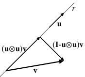
   Figure 2.9: Projected vectors.

3. For any $\alpha\in\mathbb{R},\mathbf{a},\mathbf{b}\in\mathcal{V}$ and $\mathbf{A},\mathbf{B}\in Lin(\mathcal{V})$, prove that

   $$(\alpha\mathbf{A})^{\top}=\alpha\mathbf{A}^{\top},\ \ (\mathbf{A}+\mathbf{B})^{\top}=\mathbf{A}^{\top}+\mathbf{B}^{\top},\ \ (\mathbf{a}\otimes\mathbf{b})\mathbf{A}=\mathbf{a}\otimes(\mathbf{A}^{\top}\mathbf{b}).$$

4. Prove that

   $$\mathbf{L}+\mathbf{O}=\mathbf{L}\ \ \ \forall\mathbf{L}\in Lin(\mathcal{V}).$$

5. Prove that

   $$\mathrm{tr}\mathbf{I}=3,\ \ \mathrm{tr}\mathbf{O}=0.$$

6. Prove that, $\forall\mathbf{A},\mathbf{B}\in Lin(\mathcal{V})$,

   $$\mathrm{tr}(\mathbf{A}\mathbf{B})=\mathrm{tr}(\mathbf{B}\mathbf{A}).$$

7. Prove that, $\forall\mathbf{L},\mathbf{M},\mathbf{N}\in Lin(\mathcal{V})$,

   $$\mathbf{L}^{\top}\cdot\mathbf{M}^{\top}=\mathbf{L}\cdot\mathbf{M},\ \ \mathbf{L}\mathbf{M}\cdot\mathbf{N}=\mathbf{L}\cdot\mathbf{N}\mathbf{M}^{\top}=\mathbf{M}\cdot\mathbf{L}^{\top}\mathbf{N}.$$

8. Prove the assertions in Eq. (2.4).

9. Prove that any form defined by a tensor $\mathbf{L}$ can be written as a scalar product of tensors:

   $$\mathbf{v}\cdot\mathbf{L}\mathbf{w}=\mathbf{L}\cdot\mathbf{v}\otimes\mathbf{w}\ \ \forall\mathbf{v},\mathbf{w}\in\mathcal{V},\mathbf{L}\in Lin(\mathcal{V}).$$

10. Prove that $Sym(\mathcal{V})$ and $Skw(\mathcal{V})$ are orthogonal, i.e. prove that

    $$\mathbf{A}\cdot\mathbf{B}=0\ \ \forall\mathbf{A}\in Sym(\mathcal{V}),\ \mathbf{B}\in Skw(\mathcal{V}).$$

11. For any $\mathbf{L}\in Lin(\mathcal{V})$, prove that, if $\mathbf{A}\in Sym(\mathcal{V})$, then

    $$\mathbf{A}\cdot\mathbf{L}=\mathbf{A}\cdot\mathbf{L}^{s},$$

    while if $\mathbf{B}\in Skw(\mathcal{V})$, then

    $$\mathbf{B}\cdot\mathbf{L}=\mathbf{B}\cdot\mathbf{L}^{a}.$$

12. Let $\mathbf{A},\mathbf{B},\mathbf{C},\mathbf{D}\in Lin(\mathcal{V})$; prove that

    $$\mathbf{A}\cdot(\mathbf{B}\mathbf{C}\mathbf{D})=(\mathbf{B}^{\top}\mathbf{A})\cdot(\mathbf{C}\mathbf{D})=(\mathbf{A}\mathbf{D}^{\top})\cdot(\mathbf{B}\mathbf{C}).$$

13. Prove that $\mathbf{L}\cdot\mathbf{W}=0\ \forall\mathbf{W}\in Skw(\mathcal{V})\iff\mathbf{L}\in Sym(\mathcal{V})$.

14. Express by components the second principal invariant $I_{2}$ of a tensor $\mathbf{L}$.

15. Prove that, if $\mathbf{a}=(a_{1},a_{2},a_{3}),\mathbf{b}=(b_{1},b_{2},b_{3}),\mathbf{c}=(c_{1},c_{2},c_{3})$, then

    $$\mathbf{a}\times\mathbf{b}\cdot\mathbf{c}=\det\left[\begin{array}[]{ccc}a_{1}&a_{2}&a_{3}\\ b_{1}&b_{2}&b_{3}\\ c_{1}&c_{2}&c_{3}\end{array}\right].$$

16. Prove the uniqueness of the inverse tensor.

17. Show, using the Cartesian components, that all the dyads are singular.

18. Prove that if $\mathbf{L}$ is invertible and $\alpha\in\mathbb{R}-\{0\}$ then

    $$(\alpha\mathbf{L})^{-1}=\alpha^{-1}\mathbf{L}^{-1}.$$

19. Prove that if $\mathbf{W}$ is the axial tensor of $\mathbf{w}$, then

    $$\mathbf{W}\mathbf{W}=-\frac{1}{2}|\mathbf{W}|^{2}(\mathbf{I}-\mathbf{w}\otimes\mathbf{w}).$$

20. Prove that for any two axial couples $\mathbf{w}_{1},\mathbf{W}_{1}$ and $\mathbf{w}_{2},\mathbf{W}_{2}$, we have:

    $$\mathbf{w}_{1}\cdot\mathbf{w}_{2}=\frac{1}{2}\mathbf{W}_{1}\cdot\mathbf{W}_{2}.$$

21. Prove that $\forall\mathbf{u},\mathbf{v}\in\mathcal{V},\ \mathbf{u}\times\mathbf{v}=\mathbf{o}\iff\mathbf{u}\otimes\mathbf{v}\in Sym(\mathcal{V})$.

22. Let $\mathbf{L}\in Sym(\mathcal{V})$ and positive definite and $\mathbf{R}\in Orth(\mathcal{V})^{+}$, then prove that $\mathbf{R}\mathbf{L}\mathbf{R}^{\top}\in Sym(\mathcal{V})$ and that it is positive definite.

23. Prove that the spectrum of $\mathbf{L}^{sph}$ is composed of only

    $$\lambda^{sph}=\frac{1}{3}\mathrm{tr}\mathbf{L},$$

    and that any $\mathbf{u}\in\mathcal{S}$ is an eigenvector.

24. Prove that the eigenvalues $\lambda^{dev}$ of $\mathbf{L}^{dev}$ are given by

    $$\lambda^{dev}=\lambda-\lambda^{sph},$$

    where $\lambda$ is an eigenvalue of $\mathbf{L}$.

Chapter 3 Fourth rank tensors

3.1 Fourth-rank tensors

A fourth-rank tensor $\mathbb{L}$ is any linear application from $Lin(\mathcal{V})$ to $Lin(\mathcal{V})$:

$$\mathbb{L}:Lin(\mathcal{V})\rightarrow Lin(\mathcal{V})\ |\ \mathbb{L}(\alpha_{i}\mathbf{A}_{i})=\alpha_{i}\mathbb{L}\mathbf{A}_{i}\ \forall\alpha_{i}\in\mathbb{R},\ \mathbf{A}_{i}\in Lin(\mathcal{V}),\ i=1,...,n.$$

Defining the sum of two fourth-rank tensors as

$$(\mathbb{L}_{1}+\mathbb{L}_{2})\mathbf{A}=\mathbb{L}_{1}\mathbf{A}+\mathbb{L}_{2}\mathbf{A}\ \ \forall\mathbf{A}\in Lin(\mathcal{V}),$$

the product of a scalar by a fourth-rank tensor as

$$(\alpha\mathbb{L})\mathbf{A}=\alpha(\mathbb{L}\mathbf{A})\ \ \forall\alpha\in\mathbb{R},\mathbf{A}\in Lin(\mathcal{V})$$

and the null fourth-rank tensor $\mathbb{O}$ as the unique tensor such that

$$\mathbb{O}\mathbf{A}=\mathbf{O}\ \forall\mathbf{A}\in Lin(\mathcal{V}),$$

then the set of all the tensors $\mathbb{L}$ that operate on $Lin(\mathcal{V})$ forms a vector space, denoted by $\mathbb{L}$in$(\mathcal{V})$. We define the fourth-rank identity tensor $\mathbb{I}$ as the unique tensor such that

$$\mathbb{I}\mathbf{A}=\mathbf{A}\ \ \forall\mathbf{A}\in Lin(\mathcal{V}).$$

It is apparent that the algebra of fourth-rank tensors is similar to that of second-rank tensors and, in fact, several operations with fourth-rank tensors can be introduced in almost the same way, in some sense shifting from $\mathcal{V}$ to $Lin(\mathcal{V})$ the operations. However, the algebra of fourth-rank tensors is richer than that of the second-rank ones and some care must be taken.

In the following sections, we consider some of the operations that can be done with fourth-rank tensors.

3.2 Dyads, tensor components

For any couple of tensors $\mathbf{A}$ and $\mathbf{B}\in Lin(\mathcal{V})$, the (tensor) dyad $\mathbf{A}\otimes\mathbf{B}$ is the fourth-rank tensor defined by

$$(\mathbf{A}\otimes\mathbf{B})\mathbf{L}:=\mathbf{B}\cdot\mathbf{L}\ \mathbf{A}\ \ \forall\mathbf{L}\in Lin(\mathcal{V}).$$

The application defined above is actually a fourth-rank tensor because of the bilinearity of the scalar product of second-rank tensors. Applying this rule to the nine dyads of the basis $\mathcal{B}^{2}=\{\mathbf{e}_{i}\otimes\mathbf{e}_{j},\ i,j=1,2,3\}$ of $Lin(\mathcal{V})$ leads to the introduction of the 81 fourth-rank tensors

$$\mathbf{e}_{i}\otimes\mathbf{e}_{j}\otimes\mathbf{e}_{k}\otimes\mathbf{e}_{l}:=(\mathbf{e}_{i}\otimes\mathbf{e}_{j})\otimes(\mathbf{e}_{k}\otimes\mathbf{e}_{l})$$

that form a basis, $\mathcal{B}^{4}=\{\mathbf{e}_{i}\otimes\mathbf{e}_{j}\otimes\mathbf{e}_{k}\otimes\mathbf{e}_{l},\ i,j=1,2,3\}$, for $\mathbb{L}$in$(\mathcal{V})$. We remark hence that dim$(\mathbb{L}$in$(\mathcal{V}))=81$. A useful result is that

$$(\mathbf{e}_{i}\otimes\mathbf{e}_{j}\otimes\mathbf{e}_{k}\otimes\mathbf{e}_{l})(\mathbf{e}_{p}\otimes\mathbf{e}_{q})=(\mathbf{e}_{k}\otimes\mathbf{e}_{l})\cdot(\mathbf{e}_{p}\otimes\mathbf{e}_{q})(\mathbf{e}_{i}\otimes\mathbf{e}_{j})=\delta_{kp}\delta_{lq}(\mathbf{e}_{i}\otimes\mathbf{e}_{j}).$$ (3.1)

Any fourth-rank tensor can be expressed as a linear combination (the canonical decomposition):

$$\mathbb{L}=L_{ijkl}\ \mathbf{e}_{i}\otimes\mathbf{e}_{j}\otimes\mathbf{e}_{k}\otimes\mathbf{e}_{l},\ \ i,j=1,2,3,$$

where the $L_{ijkl}$s are the 81 Cartesian components of $\mathbb{L}$ with respect to $\mathcal{B}^{4}$. The $L_{ijkl}$s are defined by the operation

$$\begin{split}(\mathbf{e}_{i}\otimes\mathbf{e}_{j})\cdot\mathbb{L}(\mathbf{e}_{k}\otimes\mathbf{e}_{l})&=(\mathbf{e}_{i}\cdot\mathbf{e}_{j})\cdot(L_{pqrs}\mathbf{e}_{p}\otimes\mathbf{e}_{q}\otimes\mathbf{e}_{r}\otimes\mathbf{e}_{s})(\mathbf{e}_{k}\otimes\mathbf{e}_{l})\\ &=(\mathbf{e}_{i}\otimes\mathbf{e}_{j})\cdot(L_{pqrs}\delta_{rk}\delta_{sl}\mathbf{e}_{p}\otimes\mathbf{e}_{q})\\ &=L_{pqrs}\delta_{rk}\delta_{sl}\delta_{ip}\delta_{jq}=L_{ijkl}.\end{split}$$

The components of a tensor dyad can be computed without any difficulty:

$$\begin{split}\mathbf{A}\otimes\mathbf{B}=(A_{ij}\mathbf{e}_{i}\otimes\mathbf{e}_{j})\otimes(B_{kl}\mathbf{e}_{k}\otimes\mathbf{e}_{l})=A_{ij}B_{kl}\mathbf{e}_{i}\otimes\mathbf{e}_{j}\otimes\mathbf{e}_{k}\otimes\mathbf{e}_{l}&\ \Rightarrow\\ (\mathbf{A}\otimes\mathbf{B})_{ijkl}=A_{ij}B_{kl}&,\end{split}$$

so that, in particular,

$$((\mathbf{a}\otimes\mathbf{b})\otimes(\mathbf{c}\otimes\mathbf{d}))_{ijkl}=a_{i}b_{j}c_{k}d_{l}.$$

Concerning the identity of $\mathbb{L}$in$(\mathcal{V})$,

$$\begin{split}I_{ijkl}=(\mathbf{e}_{i}\otimes\mathbf{e}_{l})\cdot\mathbb{I}(\mathbf{e}_{k}\otimes\mathbf{e}_{l})=(\mathbf{e}_{i}\otimes\mathbf{e}_{j})\cdot(\mathbf{e}_{k}\otimes\mathbf{e}_{l})=\mathbf{e}_{i}\cdot\mathbf{e}_{k}\mathbf{e}_{j}\cdot\mathbf{e}_{l}=\delta_{ik}\delta_{jl}&\ \Rightarrow\\ \mathbb{I}=\delta_{ik}\delta_{jl}(\mathbf{e}_{i}\otimes\mathbf{e}_{l}\otimes\mathbf{e}_{k}\otimes\mathbf{e}_{l})&.\end{split}$$

The components of $\mathbf{A}\in Lin(\mathcal{V})$, resulting from the application of $\mathbb{L}\in\mathbb{L}$in$(\mathcal{V})$ on $\mathbf{B}\in Lin(\mathcal{V})$, can now be easily calculated:

$$\begin{split}\mathbf{A}=\mathbb{L}\mathbf{B}&=L_{ijkl}(\mathbf{e}_{i}\otimes\mathbf{e}_{j}\otimes\mathbf{e}_{k}\otimes\mathbf{e}_{l})(B_{pq}\mathbf{e}_{p}\otimes\mathbf{e}_{q})\\ &=L_{ijkl}B_{pq}\delta_{kp}\delta_{lq}(\mathbf{e}_{i}\otimes\mathbf{e}_{j})\\ &=L_{ijkl}B_{kl}(\mathbf{e}_{i}\otimes\mathbf{e}_{j})\ \Rightarrow\ A_{ij}=L_{ijkl}B_{kl}.\end{split}$$ (3.2)

Moreover,

$$\begin{split}\mathbb{L}(\mathbf{A}\otimes\mathbf{B})\mathbf{C}=\mathbb{L}((\mathbf{A}\otimes\mathbf{B})\mathbf{C})=\mathbb{L}(\mathbf{B}\cdot\mathbf{C}\mathbf{A})=\mathbf{B}\cdot\mathbf{C}\ \mathbb{L}\mathbf{A}=((\mathbb{L}\mathbf{A})\otimes\mathbf{B})\mathbf{C}&\ \Rightarrow\\ \mathbb{L}(\mathbf{A}\otimes\mathbf{B})=(\mathbb{L}\mathbf{A})\otimes\mathbf{B}&.\end{split}$$

Using this result and Eq. (3.1), we can determine the components of a product of fourth-rank tensors:

$$\begin{split}\mathbb{A}\mathbb{B}&=A_{ijkl}(\mathbf{e}_{i}\otimes\mathbf{e}_{j}\otimes\mathbf{e}_{k}\otimes\mathbf{e}_{l})B_{pqrs}(\mathbf{e}_{p}\otimes\mathbf{e}_{q}\otimes\mathbf{e}_{r}\otimes\mathbf{e}_{s})\\ &=A_{ijkl}B_{pqrs}(\mathbf{e}_{i}\otimes\mathbf{e}_{j}\otimes\mathbf{e}_{k}\otimes\mathbf{e}_{l})(\mathbf{e}_{p}\otimes\mathbf{e}_{q})\otimes(\mathbf{e}_{r}\otimes\mathbf{e}_{s})\\ &=A_{ijkl}B_{pqrs}[(\mathbf{e}_{i}\otimes\mathbf{e}_{j}\otimes\mathbf{e}_{k}\otimes\mathbf{e}_{l})(\mathbf{e}_{p}\otimes\mathbf{e}_{q})]\otimes(\mathbf{e}_{r}\otimes\mathbf{e}_{s})\\ &=A_{ijkl}B_{pqrs}[\delta_{kp}\delta_{lq}(\mathbf{e}_{i}\otimes\mathbf{e}_{j})]\otimes(\mathbf{e}_{r}\otimes\mathbf{e}_{s})\\ &=A_{ijkl}B_{klrs}(\mathbf{e}_{i}\otimes\mathbf{e}_{j}\otimes\mathbf{e}_{r}\otimes\mathbf{e}_{s})\ \Rightarrow\ (\mathbb{A}\mathbb{B})_{ijrs}=A_{ijkl}B_{klrs}.\end{split}$$ (3.3)

Depending upon four indices, a fourth-rank tensor $\mathbb{L}$ cannot be represented by a matrix; however, we will see in Section 3.8 that a matrix representation of a fourth-rank tensor is still possible and that it is currently used in some cases, e.g. in elasticity.

3.3 Conjugation product, transpose, symmetries

For any two tensors $\mathbf{A},\mathbf{B}\in Lin(\mathcal{V})$ we call conjugation product the tensor $\mathbf{A}\boxtimes\mathbf{B}\in\mathbb{L}$in$(\mathcal{V})$ defined by the operation

$$(\mathbf{A}\boxtimes\mathbf{B})\mathbf{L}:=\mathbf{A}\mathbf{L}\mathbf{B}^{\top}\ \forall\mathbf{L}\in Lin(\mathcal{V}).$$

As a consequence, for the dyadic tensors of $\mathcal{B}^{2}$,

$$(\mathbf{e}_{i}\otimes\mathbf{e}_{j})\boxtimes(\mathbf{e}_{k}\otimes\mathbf{e}_{l})=\mathbf{e}_{i}\otimes\mathbf{e}_{k}\otimes\mathbf{e}_{j}\otimes\mathbf{e}_{l},$$ (3.4)

so that

$$(\mathbf{A}\boxtimes\mathbf{B})_{ijkl}=A_{ik}B_{jl}.$$

Moreover, by the uniqueness of the identity $\mathbb{I},\ \forall\mathbf{A}\in Lin(\mathcal{V})$,

$$(\mathbf{I}\boxtimes\mathbf{I})\mathbf{A}=\mathbf{I}\mathbf{A}\mathbf{I}^{\top}=\mathbf{A}\ \Rightarrow\ \mathbb{I}=\mathbf{I}\boxtimes\mathbf{I}.$$

The transpose of a fourth-rank tensor $\mathbb{L}$ is the unique tensor $\mathbb{L}^{\top}$ such that

$$\mathbf{A}\cdot(\mathbb{L}\mathbf{B})=\mathbf{B}\cdot(\mathbb{L}^{\top}\mathbf{A})\ \forall\mathbf{A},\mathbf{B}\in Lin(\mathcal{V}).$$

By this definition, setting $\mathbf{A}=\mathbf{e}_{i}\otimes\mathbf{e}_{j},\mathbf{B}=\mathbf{e}_{k}\otimes\mathbf{e}_{l}$ gives

$$(L^{\top})_{ijkl}=L_{klij}.$$

A consequence is that

$$\mathbf{A}\cdot(\mathbb{L}\mathbf{B})=\mathbf{B}\cdot(\mathbb{L}^{\top}\mathbf{A})=\mathbf{A}\cdot(\mathbb{L}^{\top})^{\top}\mathbf{B}\ \Rightarrow\ (\mathbb{L}^{\top})^{\top}=\mathbb{L}.$$

Moreover,

$$\begin{split}\mathbf{M}\cdot(\mathbf{A}\otimes\mathbf{B})^{\top}\mathbf{L}&=\mathbf{L}\cdot(\mathbf{A}\otimes\mathbf{B})\mathbf{M}\\ &=\mathbf{L}\cdot\mathbf{A}\mathbf{M}\cdot\mathbf{B}=\mathbf{M}\cdot(\mathbf{B}\mathbf{A}\cdot\mathbf{L})\\ &=\mathbf{M}\cdot(\mathbf{B}\otimes\mathbf{A})\mathbf{L}\ \Rightarrow\ (\mathbf{A}\otimes\mathbf{B})^{\top}=\mathbf{B}\otimes\mathbf{A},\end{split}$$

while, cf. Exercise 7, Chapter 2,

$$\begin{split}\mathbf{M}\cdot(\mathbf{A}\boxtimes\mathbf{B})^{\top}\mathbf{L}&=\mathbf{L}\cdot(\mathbf{A}\boxtimes\mathbf{B})\mathbf{M}\\ &=\mathbf{L}\cdot\mathbf{A}\mathbf{M}\mathbf{B}^{\top}=\mathbf{A}^{\top}\mathbf{L}\cdot\mathbf{M}\mathbf{B}^{\top}=\mathbf{M}^{\top}\mathbf{A}^{\top}\mathbf{L}\cdot\mathbf{B}^{\top}\\ &=(\mathbf{M}^{\top}\mathbf{A}^{\top}\mathbf{L})^{\top}\cdot(\mathbf{B}^{\top})^{\top}=\mathbf{L}^{\top}\mathbf{A}\mathbf{M}\cdot\mathbf{B}=\mathbf{A}\mathbf{M}\cdot\mathbf{L}\mathbf{B}\\ &=\mathbf{M}\cdot\mathbf{A}^{\top}\mathbf{L}\mathbf{B}=\mathbf{M}\cdot(\mathbf{A}^{\top}\boxtimes\mathbf{B}^{\top})\mathbf{L}\ \Rightarrow\\ &\ \ \ \ (\mathbf{A}\boxtimes\mathbf{B})^{\top}=\mathbf{A}^{\top}\boxtimes\mathbf{B}^{\top}.\end{split}$$

The property

$$(\mathbb{A}\mathbb{B})^{\top}=\mathbb{B}^{\top}\mathbb{A}^{\top}$$

can be proved in the same manner used for the analogous property of the second-rank tensors.

A tensor $\mathbb{L}\in\mathbb{L}$in$(\mathcal{V})$ is symmetric $\iff\mathbb{L}=\mathbb{L}^{\top}$. It is then evident that

$$\mathbb{L}=\mathbb{L}^{\top}\Rightarrow\ L_{ijkl}=L_{klij},$$

relations that are known as major symmetries. There are 36 major symmetries on the whole, so that a symmetric fourth-rank tensor has 45 independent components. Moreover,

$$\begin{split}&\mathbf{A}\boxtimes\mathbf{B}=(\mathbf{A}\boxtimes\mathbf{B})^{\top}=\mathbf{A}^{\top}\boxtimes\mathbf{B}^{\top}\iff\mathbf{A}=\mathbf{A}^{\top},\mathbf{B}=\mathbf{B}^{\top},\\ &\mathbf{A}\otimes\mathbf{B}=(\mathbf{A}\otimes\mathbf{B})^{\top}=\mathbf{B}\otimes\mathbf{A}\iff\mathbf{B}=\lambda\mathbf{A},\ \lambda\in\mathbb{R}.\end{split}$$

Let us now consider the case of a $\mathbb{L}\in\mathbb{L}$in$(\mathcal{V})$ such that

$$\mathbb{L}\mathbf{A}=(\mathbb{L}\mathbf{A})^{\top}\ \ \forall\mathbf{A}\in Lin(\mathcal{V}).$$

Then, by Eq. (3.2),

$$L_{ijkl}=L_{jikl},$$

relations that are called left minor symmetries: a tensor $\mathbb{L}$ having the left minor symmetries has values in $Sym(\mathcal{V})$. On the whole, the number of left minor symmetries is 27. Finally, consider the case of a $\mathbb{L}\in\mathbb{L}$in$(\mathcal{V})$ such that

$$\mathbb{L}\mathbf{A}=\mathbb{L}(\mathbf{A}^{\top})\ \ \ \forall\mathbf{A}\in Lin(\mathcal{V});$$

then, again by Eq. (3.2), we get

$$L_{ijkl}=L_{ijlk},$$

which are relations called minor right-symmetries, whose total number is also 27. It is immediate to recognize that if $\mathbb{L}$ has the minor right-symmetries, then

$$\mathbb{L}\mathbf{W}=\mathbf{O}\ \ \ \forall\mathbf{W}\in Skw(\mathcal{V}).$$

We say that a tensor has the minor symmetries if it has both the right and left minor symmetries; the total number of minor symmetries is 45, because, as can be easily checked, some of the left and right minor symmetries are the same, so finally a tensor with the minor symmetries has 36 independent components.

If $\mathbb{L}\in\mathbb{L}$in$(\mathcal{V})$ has the major and minor symmetries, then the number of independent symmetry relations is actually 60 (some minor and major symmetries coincide), so in such a case $\mathbb{L}$ depends upon 21 independent components only. This is the case, for instance, of the classical elasticity tensor.

Finally, the 6 Cauchy-Poisson symmetries are those of the type

$$L_{ijkl}=L_{ikjl}.$$

A tensor having the major, minor and Cauchy-Poisson symmetries is said to be completely symmetric, i.e. swapping any couple of indices gives an identical component. In that case, the number of independent components is only 15.

3.4 Trace and scalar product of fourth-rank tensors

We can introduce the scalar product between fourth-rank tensors in the same way we did for second-rank tensors. We first introduce the concept of trace for fourth-rank tensors, denoted by $\mathrm{tr}_{4}$, once again using the dyad (here, the tensor dyad):

$$\mathrm{tr}_{4}\mathbf{A}\otimes\mathbf{B}:=\mathbf{A}\cdot\mathbf{B}.$$

The easy proof that $\mathrm{tr}_{4}:\mathbb{L}$in$(\mathcal{V})\rightarrow\mathbb{R}$ is a linear form is based upon the properties of the scalar product of second-rank tensors and it is left to the reader. An immediate result is that

$$\mathrm{tr}_{4}\mathbf{A}\otimes\mathbf{B}=A_{ij}B_{ij},$$

Then, using the canonical decomposition, we have that

$$\mathrm{tr}_{4}\mathbb{L}=\mathrm{tr}_{4}(L_{ijkl}(\mathbf{e}_{i}\otimes\mathbf{e}_{j})\otimes(\mathbf{e}_{k}\otimes\mathbf{e}_{l}))=L_{ijkl}(\mathbf{e}_{i}\otimes\mathbf{e}_{j})\cdot(\mathbf{e}_{k}\otimes\mathbf{e}_{l})=L_{ijkl}\delta_{ik}\delta_{jl}=L_{ijij}$$

and that

$$\mathrm{tr}_{4}\mathbb{L}^{\top}=\mathrm{tr}_{4}(L_{klij}(\mathbf{e}_{i}\otimes\mathbf{e}_{j})\otimes(\mathbf{e}_{k}\otimes\mathbf{e}_{l}))=L_{klij}(\mathbf{e}_{i}\otimes\mathbf{e}_{j})\cdot(\mathbf{e}_{k}\otimes\mathbf{e}_{l})=L_{klij}\delta_{ik}\delta_{jl}=L_{ijij}=\mathrm{tr}_{4}\mathbb{L}.$$

Then, we define the scalar product of fourth-rank tensors as

$$\mathbb{A}\cdot\mathbb{B}:=\mathrm{tr}_{4}(\mathbb{A}^{\top}\mathbb{B}).$$

By the properties of $\mathrm{tr}_{4}$, the scalar product is a positive definite symmetric bilinear form:

$$\begin{split}&\alpha\mathbb{A}\cdot\beta\mathbb{B}=\mathrm{tr}_{4}(\alpha\mathbb{A}^{\top}\beta\mathbb{B})=\alpha\beta\mathrm{tr}_{4}(\mathbb{A}^{\top}\mathbb{B})=\alpha\beta\mathbb{A}\cdot\mathbb{B},\\ &\mathbb{A}\cdot\mathbb{B}=\mathrm{tr}_{4}(\mathbb{A}^{\top}\mathbb{B})=\mathrm{tr}_{4}(\mathbb{A}^{\top}\mathbb{B})^{\top}=\mathrm{tr}_{4}(\mathbb{B}^{\top}\mathbb{A})=\mathbb{B}\cdot\mathbb{A},\\ &\mathbb{A}\cdot\mathbb{A}=\mathrm{tr}_{4}(\mathbb{A}^{\top}\mathbb{A})=(\mathbb{A}^{\top}\mathbb{A})_{ijij}=A_{klij}A_{klij}>0\ \forall\mathbb{A}\in{\mathbb{L}}in(\mathcal{V}),\mathbb{A}\cdot\mathbb{A}=0\iff\mathbb{A}=\mathbb{O}.\end{split}$$

By components

$$\begin{split}\mathbb{A}\cdot\mathbb{B}&=\mathrm{tr}_{4}((A_{klij}\mathbf{e}_{i}\otimes\mathbf{e}_{j}\otimes\mathbf{e}_{k}\otimes\mathbf{e}_{l})(B_{pqrs}\mathbf{e}_{p}\otimes\mathbf{e}_{q}\otimes\mathbf{e}_{r}\otimes\mathbf{e}_{s}))\\ &=\mathrm{tr}_{4}(A_{klij}B_{pqrs}\delta_{kp}\delta_{lq}(\mathbf{e}_{i}\otimes\mathbf{e}_{j})\otimes(\mathbf{e}_{r}\otimes\mathbf{e}_{s}))\\ &=A_{klij}B_{pqrs}\delta_{kp}\delta_{lq}(\mathbf{e}_{i}\otimes\mathbf{e}_{j})\cdot(\mathbf{e}_{r}\otimes\mathbf{e}_{s})=A_{klij}B_{pqrs}\delta_{kp}\delta_{lq}\delta_{ir}\delta_{js}=A_{klij}B_{klij}.\end{split}$$

The rule for computing the scalar product is hence always the same, as was already seen for vectors and second-rank tensors: All the indexes are to be saturated.

In complete analogy with vectors and second-rank tensors, we say that $\mathbb{A}$ is orthogonal to $\mathbb{B}\iff$

$$\mathbb{A}\cdot\mathbb{B}=0$$

and we define the norm of $\mathbb{L}$ as

$$|\mathbb{L}|:=\sqrt{\mathbb{L}\cdot\mathbb{L}}=\sqrt{\mathrm{tr}_{4}\mathbb{L}^{\top}\mathbb{L}}=\sqrt{L_{ijkl}L_{ijkl}}.$$

3.5 Projectors, identities

For the spherical part of any $\mathbf{A}\in Sym(\mathcal{V})$ we can write

$$\mathbf{A}^{sph}:=\frac{1}{3}\mathrm{tr}\mathbf{A}\ \mathbf{I}=\frac{1}{3}\mathbf{I}\cdot\mathbf{A}\ \mathbf{I}=\frac{1}{3}(\mathbf{I}\otimes\mathbf{I})\mathbf{A}=\mathbb{S}^{sph}\mathbf{A},$$

where

$$\mathbb{S}^{sph}:=\frac{1}{3}\mathbf{I}\otimes\mathbf{I}$$

is the spherical projector, i.e. the fourth-rank tensor that extracts from any $\mathbf{A}\in Lin(\mathcal{V})$ its spherical part. Moreover,

$$\mathbf{A}^{dev}:=\mathbf{A}-\mathbf{A}^{sph}=\mathbb{I}\mathbf{A}-\mathbb{S}^{sph}\mathbf{A}=\mathbb{D}^{dev}\mathbf{A},$$

where

$$\mathbb{D}^{dev}:=\mathbb{I}-\mathbb{S}^{sph}$$

is the deviatoric projector, i.e. the fourth-rank tensor that extracts from any $\mathbf{A}\in Lin(\mathcal{V})$ its deviatoric part. It is worth noting that

$$\mathbb{I}=\mathbb{S}^{sph}+\mathbb{D}^{dev}.$$

Moreover, about the components of $\mathbb{S}^{sph}$,

$$\begin{split}S^{sph}_{ijkl}&=(\mathbf{e}_{i}\otimes\mathbf{e}_{j})\cdot\frac{1}{3}(\mathbf{I}\otimes\mathbf{I})(\mathbf{e}_{k}\otimes\mathbf{e}_{l})=\frac{1}{3}\mathbf{I}\cdot(\mathbf{e}_{i}\otimes\mathbf{e}_{j})\ \mathbf{I}\cdot(\mathbf{e}_{k}\otimes\mathbf{e}_{l})\\ &=\frac{1}{3}\mathrm{tr}(\mathbf{e}_{i}\otimes\mathbf{e}_{j})\mathrm{tr}(\mathbf{e}_{k}\otimes\mathbf{e}_{l})=\frac{1}{3}\delta_{ij}\delta_{kl}\ \rightarrow\ \mathbb{S}^{sph}=\frac{1}{3}\delta_{ij}\delta_{kl}(\mathbf{e}_{i}\otimes\mathbf{e}_{j}\otimes\mathbf{e}_{k}\otimes\mathbf{e}_{l}).\end{split}$$

We remark that

$$\mathbb{S}^{sph}=(\mathbb{S}^{sph})^{\top}.$$

We introduce now the tensor $\mathbb{I}^{s}$, restriction of $\mathbb{I}$ to $\mathbf{A}\in Sym(\mathcal{V})$. It can be introduced as follows: $\forall\mathbf{A}\in Sym(\mathcal{V})$

$$\mathbf{A}=\frac{1}{2}(\mathbf{A}+\mathbf{A}^{\top}),$$

and

$$\mathbf{A}=\mathbb{I}\mathbf{A}=\frac{1}{2}(\mathbb{I}\mathbf{A}+\mathbb{I}\mathbf{A}^{\top})=\frac{1}{2}(I_{ijkl}A_{kl}+I_{ijkl}A_{lk})(\mathbf{e}_{i}\otimes\mathbf{e}_{j}\otimes\mathbf{e}_{k}\otimes\mathbf{e}_{l});$$

because $\mathbf{A}=\mathbf{A}^{\top}$, there is insensitivity to the swap of indexes $k$ and $l$, so

$$\mathbf{A}=\frac{1}{2}(I_{ijkl}A_{kl}+I_{ijlk}A_{lk})(\mathbf{e}_{i}\otimes\mathbf{e}_{j}\otimes\mathbf{e}_{k}\otimes\mathbf{e}_{l})=\frac{1}{2}(\delta_{ik}\delta_{jl}+\delta_{il}\delta_{jk})A_{kl}(\mathbf{e}_{i}\otimes\mathbf{e}_{j}\otimes\mathbf{e}_{k}\otimes\mathbf{e}_{l}).$$

Then, if we admit the interchangeability of indexes $k$ and $l$, i.e. if we postulate the existence of the minor right-symmetries for $\mathbb{I}$, then $\mathbb{I}=\mathbb{I}^{s}$, with

$$\mathbb{I}^{s}=\frac{1}{2}(\delta_{ik}\delta_{jl}+\delta_{il}\delta_{jk})(\mathbf{e}_{i}\otimes\mathbf{e}_{j}\otimes\mathbf{e}_{k}\otimes\mathbf{e}_{l}).$$

It is apparent that

$$I^{s}_{ijkl}=I^{s}_{klij},$$

i.e. $\mathbb{I}^{s}=(\mathbb{I}^{s})^{\top}$, but also that

$$I^{s}_{ijkl}=\frac{1}{2}(\delta_{il}\delta_{jk}+\delta_{ik}\delta_{jl})=I^{s}_{jikl},$$

i.e., $\mathbb{I}^{s}$ has also the minor left-symmetries; in other words, $\mathbb{I}^{s}$ has the major and minor symmetries, like an elasticity tensor, while this is not the case for $\mathbb{I}$. In fact

$$I_{ijkl}=I_{jilk}=\delta_{ik}\delta_{jl}\neq\delta_{il}\delta_{jk}=I_{jikl}=I_{ijlk}.$$

Because $\mathbb{S}^{sph}$ and $\mathbb{D}^{dev}$ operate on $Sym(\mathcal{V})$, it is immediate to recognize that it is also

$$\mathbb{D}^{dev}=\mathbb{I}^{s}-\mathbb{S}^{sph}\ \Rightarrow\ \mathbb{I}^{s}=\mathbb{S}^{sph}+\mathbb{D}^{dev}.$$

It is worth noting that

$$(\mathbb{D}^{dev})^{\top}=(\mathbb{I}^{s}-\mathbb{S}^{sph})^{\top}=(\mathbb{I}^{s})^{\top}-(\mathbb{S}^{sph})^{\top}=\mathbb{I}^{s}-\mathbb{S}^{sph}=\mathbb{D}^{dev}.$$

We can now determine the components of $\mathbb{D}^{dev}$:

$$\begin{split}&D^{dev}_{ijkl}=I^{s}_{ijkl}-S^{sph}_{ijkl}=\frac{1}{2}(\delta_{ik}\delta_{jl}+\delta_{il}\delta_{jk})-\frac{1}{3}\delta_{ij}\delta_{kl}\ \rightarrow\\ &\mathbb{D}^{dev}=\left[\frac{1}{2}(\delta_{ik}\delta_{jl}+\delta_{il}\delta_{jk})-\frac{1}{3}\delta_{ij}\delta_{kl}\right](\mathbf{e}_{i}\otimes\mathbf{e}_{j}\otimes\mathbf{e}_{k}\otimes\mathbf{e}_{l}).\end{split}$$

We remark that the result (2.9) implies that $\mathbb{S}^{sph}$ and $\mathbb{D}^{dev}$ are orthogonal projectors, i.e. they project the same $\mathbf{A}\in Sym(\mathcal{V})$ into two orthogonal subspaces of $\mathcal{V}$, $Sph(\mathcal{V})$ and $Dev(\mathcal{V})$.

The tensor $\mathbb{T}^{trp}\in\mathbb{L}$in$(\mathcal{V})$ defined by the operation

$$\mathbb{T}^{trp}\mathbf{A}=\mathbf{A}^{\top}\ \ \ \forall\mathbf{A}\in Lin(\mathcal{V}),$$

is the transposition projector, whose components are

$$T^{trp}_{ijkl}=(\mathbf{e}_{i}\otimes\mathbf{e}_{j})\cdot\mathbb{T}^{trp}(\mathbf{e}_{k}\otimes\mathbf{e}_{l})=(\mathbf{e}_{i}\otimes\mathbf{e}_{j})\cdot(\mathbf{e}_{l}\otimes\mathbf{e}_{k})=\delta_{il}\delta_{jk}.$$

The following operation defines the symmetry projector $\mathbb{S}^{sym}\in\mathbb{L}$in$(\mathcal{V})$:

$$\mathbb{S}^{sym}\mathbf{A}=\frac{1}{2}(\mathbf{A}+\mathbf{A}^{\top})\ \forall\mathbf{A}\in Lin(\mathcal{V}),$$

while the antisymmetry projector $\mathbb{W}^{skw}\in\mathbb{L}$in$(\mathcal{V})$ is defined by

$$\mathbb{W}^{skw}\mathbf{A}=\frac{1}{2}(\mathbf{A}-\mathbf{A}^{\top})\ \forall\mathbf{A}\in Lin(\mathcal{V}).$$

Also $\mathbb{S}^{sym}$ and $\mathbb{W}^{skw}$ are orthogonal projectors, because they project the same $\mathbf{A}\in Lin(\mathcal{V})$ into two orthogonal subspaces of $Lin(\mathcal{V})$: $Sym(\mathcal{V})$ and $Skw(\mathcal{V})$, see Exercise 10, Chapter 2.

We prove now two properties of the projectors: $\forall\mathbf{A}\in Lin(\mathcal{V})$,

$$(\mathbb{S}^{sym}+\mathbb{W}^{skw})\mathbf{A}=\frac{1}{2}(\mathbf{A}+\mathbf{A}^{\top})+\frac{1}{2}(\mathbf{A}-\mathbf{A}^{\top})=\mathbf{A}=\mathbb{I}\mathbf{A}\ \Rightarrow\ \mathbb{S}^{sym}+\mathbb{W}^{skw}=\mathbb{I}.$$ (3.5)

Then,

$$(\mathbb{S}^{sym}-\mathbb{W}^{skw})\mathbf{A}=\frac{1}{2}(\mathbf{A}+\mathbf{A}^{\top})-\frac{1}{2}(\mathbf{A}-\mathbf{A}^{\top})=\mathbf{A}^{\top}=\mathbb{T}^{trp}\mathbf{A}\ \Rightarrow\ \mathbb{S}^{sym}-\mathbb{W}^{skw}=\mathbb{T}^{trp}.$$ (3.6)

3.6 Orthogonal conjugator

For any $\mathbf{U}\in Orth(\mathcal{V})$, we define its orthogonal conjugator $\mathbb{U}\in\mathbb{L}$in$(\mathcal{V})$ as

$$\mathbb{U}:=\mathbf{U}\boxtimes\mathbf{U}.$$

Theorem 22.

(Orthogonality of $\mathbb{U}$). The orthogonal conjugator is an orthogonal tensor of $\mathbb{L}$in$(\mathcal{V})$, i.e. it preserves the scalar product between tensors:

$$\mathbb{U}\mathbf{A}\cdot\mathbb{U}\mathbf{B}=\mathbf{A}\cdot\mathbf{B}\ \ \forall\mathbf{A},\mathbf{B}\in Lin(\mathcal{V}).$$

Proof.

By the assertion in Exercise 12 of Chapter 2 and because $\mathbf{U}\in Orth(\mathcal{V})$, we have

$$\begin{split}\mathbb{U}\mathbf{A}\cdot\mathbb{U}\mathbf{B}&=(\mathbf{U}\boxtimes\mathbf{U})\mathbf{A}\cdot(\mathbf{U}\boxtimes\mathbf{U})\mathbf{B}=\mathbf{U}\mathbf{A}\mathbf{U}^{\top}\cdot\mathbf{U}\mathbf{B}\mathbf{U}^{\top}\\ &=\mathbf{U}^{\top}\mathbf{U}\mathbf{A}\mathbf{U}^{\top}\cdot\mathbf{B}\mathbf{U}^{\top}=\mathbf{A}\mathbf{U}^{\top}\cdot\mathbf{B}\mathbf{U}^{\top}=\mathbf{A}\mathbf{U}^{\top}\mathbf{U}\cdot\mathbf{B}=\mathbf{A}\cdot\mathbf{B}.\end{split}$$

∎

Just as for tensors of $Orth(\mathcal{V})$, we also have

$$\mathbb{U}\mathbb{U}^{\top}=\mathbb{U}^{\top}\mathbb{U}=\mathbb{I}.$$

In fact, see the assertion in Exercise 4:

$$\mathbb{U}\mathbb{U}^{\top}=(\mathbf{U}\boxtimes\mathbf{U})(\mathbf{U}^{\top}\boxtimes\mathbf{U}^{\top})=\mathbf{U}\mathbf{U}^{\top}\boxtimes\mathbf{U}\mathbf{U}^{\top}=\mathbf{I}\boxtimes\mathbf{I}=\mathbb{I}.$$ (3.7)

The orthogonal conjugators also have some properties in relation with projectors:

Theorem 23.

$\mathbb{S}^{sph}$ is unaffected by any orthogonal conjugator, while $\mathbb{D}^{dev}$ commutes with any orthogonal conjugator.

Proof.

For any $\mathbf{L}\in Sym(\mathcal{V})$ and $\mathbf{U}\in Orth(\mathcal{V})$,

$$\begin{split}\mathbb{U}\mathbb{S}^{sph}\mathbf{L}&=(\mathbf{U}\boxtimes\mathbf{U})\left(\frac{1}{3}\mathbf{I}\otimes\mathbf{I}\right)\mathbf{L}=\frac{1}{3}(\mathrm{tr}\mathbf{L})(\mathbf{U}\boxtimes\mathbf{U})\mathbf{I}=\frac{1}{3}(\mathrm{tr}\mathbf{L})\mathbf{U}\mathbf{I}\mathbf{U}^{\top}\\ &=\frac{1}{3}(\mathrm{tr}\mathbf{L})\mathbf{I}=\frac{1}{3}\mathbf{I}\cdot\mathbf{L}\ \mathbf{I}=\frac{1}{3}(\mathbf{I}\otimes\mathbf{I})\mathbf{L}=\mathbb{S}^{sph}\mathbf{L}.\end{split}$$

Moreover,

$$\begin{split}\mathbb{S}^{sph}\mathbb{U}\mathbf{L}&=\left(\frac{1}{3}\mathbf{I}\otimes\mathbf{I}\right)(\mathbf{U}\boxtimes\mathbf{U})\mathbf{L}=\frac{1}{3}(\mathbf{I}\otimes\mathbf{I})(\mathbf{U}\mathbf{L}\mathbf{U}^{\top})=\frac{1}{3}(\mathbf{I}\cdot\mathbf{U}\mathbf{L}\mathbf{U}^{\top})\mathbf{I}\\ &=\frac{1}{3}\mathrm{tr}(\mathbf{U}\mathbf{L}\mathbf{U}^{\top})\mathbf{I}=\frac{1}{3}\mathrm{tr}(\mathbf{U}^{\top}\mathbf{U}\mathbf{L})\mathbf{I}=\frac{1}{3}(\mathrm{tr}\mathbf{L})\mathbf{I}=\frac{1}{3}\mathbf{I}\cdot\mathbf{L}\mathbf{I}=\frac{1}{3}(\mathbf{I}\otimes\mathbf{I})\mathbf{L}=\mathbb{S}^{sph}\mathbf{L}.\end{split}$$

Thus, we have proved that

$$\mathbb{S}^{sph}\mathbb{U}=\mathbb{U}\mathbb{S}^{sph}=\mathbb{S}^{sph},$$

i.e. that the spherical projector $\mathbb{S}^{sph}$ is unaffected by any orthogonal conjugator. Furthermore

$$\mathbb{D}^{dev}\mathbb{U}\mathbf{L}=(\mathbb{I}^{s}-\mathbb{S}^{sph})\mathbb{U}\mathbf{L}=\mathbb{I}^{s}\mathbb{U}\mathbf{L}-\mathbb{S}^{sph}\mathbb{U}\mathbf{L}=\mathbb{U}\mathbf{L}-\mathbb{S}^{sph}\mathbf{L}=(\mathbb{U}-\mathbb{S}^{sph})\mathbf{L}$$

and

$$\mathbb{U}\mathbb{D}^{dev}\mathbf{L}=\mathbb{U}(\mathbb{I}^{s}-\mathbb{S}^{sph})\mathbf{L}=\mathbb{U}\mathbb{I}^{s}\mathbf{L}-\mathbb{U}\mathbb{S}^{sph}\mathbf{L}=\mathbb{U}\mathbf{L}-\mathbb{S}^{sph}\mathbf{L}=(\mathbb{U}-\mathbb{S}^{sph})\mathbf{L},$$

so that

$$\mathbb{D}^{dev}\mathbb{U}=\mathbb{U}\mathbb{D}^{dev}.$$

∎

3.7 Rotations and symmetries

We ponder now how to rotate a fourth-rank tensor, i.e., what are the components of

$$\mathbb{L}=L_{ijkl}\mathbf{e}_{i}\otimes\mathbf{e}_{j}\otimes\mathbf{e}_{k}\otimes\mathbf{e}_{l}$$

in a basis $\mathcal{B}^{\prime}=\{\mathbf{e}_{1}^{\prime},\mathbf{e}_{2}^{\prime},\mathbf{e}_{3}^{\prime}\}$ obtained rotating the basis $\mathcal{B}=\{\mathbf{e}_{1},\mathbf{e}_{2},\mathbf{e}_{3}\}$ by the rotation $\mathbb{R}=R_{ij}\mathbf{e}_{i}\otimes\mathbf{e}_{j},\mathbb{R}\in Orth(\mathcal{V})^{+}$. The procedure is exactly the same already followed for vectors and second-rank tensors:

$$\begin{split}\mathbb{L}&=L_{ijkl}\mathbf{e}_{i}\otimes\mathbf{e}_{j}\otimes\mathbf{e}_{k}\otimes\mathbf{e}_{l}=L_{ijkl}R^{\top}_{pi}\mathbf{e}_{p}^{\prime}\otimes R^{\top}_{qj}\mathbf{e}_{q}^{\prime}\otimes R^{\top}_{rk}\mathbf{e}_{r}^{\prime}\otimes R^{\top}_{sl}\mathbf{e}_{s}^{\prime}\\ &=R^{\top}_{pi}R^{\top}_{qj}R^{\top}_{rk}R^{\top}_{sl}L_{ijkl}\mathbf{e}_{p}^{\prime}\otimes\mathbf{e}_{q}^{\prime}\otimes\mathbf{e}_{r}^{\prime}\otimes\mathbf{e}_{s}^{\prime},\end{split}$$

i.e.

$$L_{pqrs}^{\prime}=R^{\top}_{pi}R^{\top}_{qj}R^{\top}_{rk}R^{\top}_{sl}L_{ijkl}.$$

We see clearly that the components of $\mathbb{L}$ in the basis $\mathcal{B}^{\prime}$ are a linear combination of those in $\mathcal{B}$, the coefficients of the linear combination being fourth powers of the director cosines, the $R_{ij}$s. The introduction of the orthogonal conjugator of the rotation $\mathbf{R}$,

$$\mathbb{R}=\mathbf{R}\boxtimes\mathbf{R},$$

allows us to give a compact expression for the rotation of second- and fourth-rank tensors (for completeness we recall also that of a vector $\mathbf{w}$);

$$\begin{array}[]{c}\mathbf{w}^{\prime}=\mathbf{R}^{\top}\mathbf{w},\vskip 6.0pt plus 2.0pt minus 2.0pt\\ \mathbf{L}^{\prime}=\mathbf{R}^{\top}\mathbf{L}\mathbf{R}=(\mathbf{R}^{\top}\boxtimes\mathbf{R}^{\top})\mathbf{L}=\mathbb{R}^{\top}\mathbf{L},\vskip 6.0pt plus 2.0pt minus 2.0pt\\ \mathbb{L}^{\prime}=(\mathbf{R}^{\top}\boxtimes\mathbf{R}^{\top})\mathbb{L}(\mathbf{R}\boxtimes\mathbf{R})=\mathbb{R}^{\top}\mathbb{L}\mathbb{R}.\end{array}$$

Checking the above relations with the orthogonal conjugator $\mathbb{R}$ is left to the reader. It is worth noting that, actually, these transformations are valid not only for $\mathbf{R}\in Orth(\mathcal{V})^{+}$, but more generally for any $\mathbf{U}\in Orth(\mathcal{V})$, i.e. also for symmetries.

If $\mathbf{U}$ denotes the tensor of change of basis under any orthogonal transformation, i.e. if we put $\mathbf{U}=\mathbf{R}^{\top}$ for the rotations, then the above relations become

$$\begin{array}[]{c}\mathbf{w}^{\prime}=\mathbf{U}\mathbf{w},\vskip 6.0pt plus 2.0pt minus 2.0pt\\ \mathbf{L}^{\prime}=\mathbf{U}\mathbf{L}\mathbf{U}^{\top}=(\mathbf{U}\boxtimes\mathbf{U})\mathbf{L}=\mathbb{U}\mathbf{L},\vskip 6.0pt plus 2.0pt minus 2.0pt\\ \mathbb{L}^{\prime}=(\mathbf{U}\boxtimes\mathbf{U})\mathbb{L}(\mathbf{U}\boxtimes\mathbf{U})^{\top}=\mathbb{U}\mathbb{L}\mathbb{U}^{\top}.\end{array}$$ (3.8)

Finally, we say that $\mathbf{L}\in Lin(\mathcal{V})$ or $\mathbb{L}\in\mathbb{L}$in$(\mathcal{V})$ is invariant under an orthogonal transformation $\mathbf{U}$ if

$$\mathbf{U}\mathbf{L}\mathbf{U}^{\top}=\mathbf{L},\ \ \ \mathbb{U}\mathbb{L}\mathbb{U}^{\top}=\mathbb{L};$$

right multiplying both terms by $\mathbf{U}$ or by $\mathbb{U}$ and through Eq. (3.7), we get that $\mathbf{L}$ or $\mathbb{L}$ are invariant under $\mathbf{U}\iff$

$$\mathbf{U}\mathbf{L}=\mathbf{L}\mathbf{U},\ \ \ \mathbb{U}\mathbb{L}=\mathbb{L}\mathbb{U},$$

i.e. $\iff\mathbf{L}$ and $\mathbf{U}$, or $\mathbb{L}$ and $\mathbb{U}$ commute. This relation allows, for example, the analysis of material symmetries in anisotropic elasticity.

If a tensor is invariant under any orthogonal transformation, i.e. if the previous equations hold true $\forall\mathbf{U}\in Orth(\mathcal{V})$, then the tensor is said to be isotropic. A general result is that a fourth-rank tensor $\mathbb{L}$ is isotropic $\iff$ there exist two scalar functions $\lambda,\mu$ such that

$$\mathbb{L}\mathbf{A}=2\mu\mathbf{A}+\lambda\mathrm{tr}\mathbf{A}\ \mathbf{I}\ \ \ \forall\mathbf{A}\in Sym(\mathcal{V}).$$

The reader is referred to the book of Gurtin (see the references) for the proof of this result and for a deeper insight into isotropic functions.

3.8 The Kelvin formalism

As already mentioned, though fourth-rank tensors cannot be organized in and represented by a matrix, nevertheless a matrix formalism for these operators exists. Such formalism is due to Kelvin and it is strictly related to the theory of elasticity, i.e. it concerns the Cauchy’s stress tensor $\boldsymbol{\sigma}$, the strain tensor $\boldsymbol{\varepsilon}$ and the elasticity tensor $\mathbb{E}$. The relation between $\boldsymbol{\sigma}$ and $\boldsymbol{\varepsilon}$ is given by the celebrated (generalized) Hooke’s law:

$$\boldsymbol{\sigma}=\mathbb{E}\boldsymbol{\varepsilon}.$$

Both $\boldsymbol{\sigma},\boldsymbol{\varepsilon}\in Sym(\mathcal{V})$ while $\mathbb{E}=\mathbb{E}^{\top}$ and it has also the minor symmetries, so $\mathbb{E}$ has just 21 independent components. In the Kelvin formalism, the six independent components of $\boldsymbol{\sigma}$ and $\boldsymbol{\varepsilon}$ are organized into column vectors and renumbered as follows

$$\{\sigma\}=\left\{\begin{array}[]{c}\sigma_{1}=\sigma_{11}\\ \sigma_{2}=\sigma_{22}\\ \sigma_{3}=\sigma_{33}\\ \sigma_{4}=\sqrt{2}\sigma_{23}\\ \sigma_{5}=\sqrt{2}\sigma_{31}\\ \sigma_{6}=\sqrt{2}\sigma_{12}\end{array}\right\},\ \ \ \{\varepsilon\}=\left\{\begin{array}[]{c}\varepsilon_{1}=\varepsilon_{11}\\ \varepsilon_{2}=\varepsilon_{22}\\ \varepsilon_{3}=\varepsilon_{33}\\ \varepsilon_{4}=\sqrt{2}\varepsilon_{23}\\ \varepsilon_{5}=\sqrt{2}\varepsilon_{31}\\ \varepsilon_{6}=\sqrt{2}\varepsilon_{12}\end{array}\right\}.$$

The elasticity tensor $\mathbb{E}$ is reduced to a $6\times 6$ matrix $[E]$ as a consequence of the minor symmetries induced by the symmetry of $\boldsymbol{\sigma}$ and $\boldsymbol{\varepsilon}$; this matrix is symmetric because $\mathbb{E}=\mathbb{E}^{\top}$:

$$[E]=\left[\begin{array}[]{cccccc}E_{11}=E_{1111}&E_{12}=E_{1122}&E_{13}=E_{1133}&E_{14}=\sqrt{2}E_{1123}&E_{15}=\sqrt{2}E_{1131}&E_{16}=\sqrt{2}E_{1112}\\ E_{12}=E_{1122}&E_{22}=E_{2222}&E_{23}=E_{2233}&E_{24}=\sqrt{2}E_{2223}&E_{25}=\sqrt{2}E_{2231}&E_{26}=\sqrt{2}E_{2212}\\ E_{13}=E_{1133}&E_{23}=E_{2233}&E_{33}=E_{3333}&E_{34}=\sqrt{2}E_{3323}&E_{35}=\sqrt{2}E_{3331}&E_{36}=\sqrt{2}E_{3312}\\ E_{14}=\sqrt{2}E_{1123}&E_{24}=\sqrt{2}E_{2223}&E_{34}=\sqrt{2}E_{3323}&E_{44}=2E_{2323}&E_{45}=2E_{2331}&E_{46}=2E_{2312}\\ E_{15}=\sqrt{2}E_{1131}&E_{25}=\sqrt{2}E_{2231}&E_{35}=\sqrt{2}E_{3331}&E_{45}=2E_{2331}&E_{55}=2E_{3131}&E_{56}=2E_{3112}\\ E_{16}=\sqrt{2}E_{1112}&E_{26}=\sqrt{2}E_{2212}&E_{36}=\sqrt{2}E_{3312}&E_{46}=2E_{2312}&E_{56}=2E_{3112}&E_{66}=2E_{1212}\end{array}\right].$$

In this way, the matrix product

$$\{\sigma\}=[E]\{\varepsilon\}$$ (3.9)

is equivalent to the tensor form of the Hooke’s law and all the operations can be done by the aid of classical matrix algebra, e.g. the computation of the inverse of $\mathbb{E}$, the compliance tensor.

An important operation is the expression of tensor $\mathbb{U}$ in Eq. (3.8) in the Kelvin formalism; some tedious but straightforward passages give the result:

$$[U]=\small\left[\begin{array}[]{cccccc}U^{2}_{11}&U^{2}_{12}&U^{2}_{13}&\sqrt{2}U_{12}U_{13}&\sqrt{2}U_{13}U_{11}&\sqrt{2}U_{11}U_{12}\\ U^{2}_{21}&U^{2}_{22}&U^{2}_{23}&\sqrt{2}U_{22}U_{23}&\sqrt{2}U_{23}U_{21}&\sqrt{2}U_{21}U_{22}\\ U^{2}_{31}&U^{2}_{32}&U^{2}_{33}&\sqrt{2}U_{32}U_{33}&\sqrt{2}U_{33}U_{31}&\sqrt{2}U_{31}U_{32}\\ \sqrt{2}U_{21}U_{31}&\sqrt{2}U_{22}U_{32}&\sqrt{2}U_{23}U_{33}&U_{23}U_{32}+U_{22}U_{33}&U_{33}U_{21}+U_{31}U_{23}&U_{31}U_{22}+U_{32}U_{21}\\ \sqrt{2}U_{31}U_{11}&\sqrt{2}U_{32}U_{12}&\sqrt{2}U_{33}U_{13}&U_{32}U_{13}+U_{33}U_{12}&U_{31}U_{13}+U_{33}U_{11}&U_{31}U_{12}+U_{32}U_{11}\\ \sqrt{2}U_{11}U_{21}&\sqrt{2}U_{12}U_{22}&\sqrt{2}U_{13}U_{23}&U_{12}U_{23}+U_{13}U_{22}&U_{11}U_{23}+U_{13}U_{21}&U_{11}U_{22}+U_{12}U_{21}\end{array}\right]$$

With some work, it can be checked that

$$[U][U]^{\top}=[U]^{\top}[U]=[I],$$

i.e. that $[U]$ is an orthogonal matrix in $\mathbb{R}^{6}$. Of course,

$$[R]=[U]^{\top}$$

is the matrix that in the Kelvin formalism represents the tensor $\mathbf{R}=\mathbf{U}^{\top}$. The change of basis for $\boldsymbol{\sigma}$ and $\boldsymbol{\varepsilon}$ are hence done through the relations

$$\{\sigma^{\prime}\}=[U]\{\sigma\},\ \ \ \{\varepsilon^{\prime}\}=[U]\{\varepsilon\},$$

which applied to Eq. (3.9) give

$$\{\sigma\}=[E]\{\varepsilon\}\ \rightarrow\ [U]^{\top}\{\sigma^{\prime}\}=[E][U]^{\top}\{\varepsilon^{\prime}\}\ \rightarrow\ \{\sigma^{\prime}\}=[U][E][U]^{\top}\{\varepsilon^{\prime}\}$$

i.e. in the basis $\mathcal{B}^{\prime}$

$$\{\sigma^{\prime}\}=[E^{\prime}]\{\varepsilon^{\prime}\},$$

where

$$[E^{\prime}]=[U][E][U]^{\top}=[R]^{\top}[E][R]$$

is the matrix representing $\mathbb{E}$ in $\mathcal{B}^{\prime}$ in the Kelvin formalism. Though it is possible to give the expression of the components of $[E^{\prime}]$, they are so long that they are omitted here.

3.9 The polar formalism for plane tensors

The Cartesian representation of tensors makes use of quantities that are basis-dependent, and the change of basis implies algebraic transformations rather complicate. The question of representing tensors using other quantities than Cartesian components is hence of importance. In particular, it should be interesting to represent a tensor making use of only invariants of the tensor itself and of angles, the simplest geometrical way to determine a direction.

In the case of plane tensors this has been done by Verchery who introduced the so-called polar formalism. This is basically a mathematical technique to find the invariants of a tensor of any rank. Here, we give just a short insight into the polar formalism of fourth-rank tensors of the elastic type, i.e. having the minor and major symmetries, omitting the proof of the results.

The Cartesian components of a plane fourth-rank elasticity-type tensor $\mathbb{T}$ in a frame rotated through an angle $\theta$ can be expressed as

$$\begin{split}&T_{1111}=T_{0}+2T_{1}+R_{0}\cos 4(\varPhi_{0}-\theta)+4R_{1}\cos 2(\varPhi_{1}-\theta),\\ &T_{1112}=R_{0}\sin 4(\varPhi_{0}-\theta)+2R_{1}\sin 2(\varPhi_{1}-\theta),\\ &T_{1122}=-T_{0}+2T_{1}-R_{0}\cos 4(\varPhi_{0}-\theta),\\ &T_{1212}=T_{0}-R_{0}\cos 4(\varPhi_{0}-\theta),\\ &T_{1222}=-R_{0}\sin 4(\varPhi_{0}-\theta)+2R_{1}\sin 2(\varPhi_{1}-\theta),\\ &T_{2222}=T_{0}+2T_{1}+R_{0}\cos 4(\varPhi_{0}-\theta)-4R_{1}\cos 2(\varPhi_{1}-\theta).\end{split}$$

In the above equations, $T_{0},T_{1},R_{0},R_{1}$ are tensor invariants, with all of them non negative, while $\varPhi_{0}$ and $\varPhi_{1}$ are angles whose difference, $\varPhi_{0}-\varPhi_{1}$, is also a tensor invariant, so fixing one of the two polar angles corresponds to fixing a frame. In particular, the tensor invariants have a direct physical meaning (e.g., for the elasticity tensor, they are linked to material symmetries and to strain energy decomposition). We remark also that the change of frame is extremely simple in the polar formalism: It is sufficient to subtract the angle $\theta$ formed by the new frame from the two polar angles.

The Cartesian expression of the polar invariants can be found inverting the previous expressions:

$$\begin{split}&T_{0}=\frac{1}{8}(T_{1111}-2T_{1122}+4T_{1212}+T_{2222}),\\ &T_{1}=\frac{1}{8}(T_{1111}+2T_{1122}+T_{2222}),\\ &R_{0}=\frac{1}{8}\sqrt{(T_{1111}-2T_{1122}-4T_{1212}+T_{2222})^{2}+16(T_{1112}-T_{1222})^{2}},\\ &R_{1}=\frac{1}{8}\sqrt{(T_{1111}-T_{2222})^{2}+4(T_{1112}+T_{1222})^{2}},\\ &\tan 4\varPhi_{0}=\frac{4(T_{1112}-T_{1222})}{T_{1111}-2T_{1122}-4T_{1212}+T_{2222}},\\ &\tan 2\varPhi_{1}=\frac{2(T_{1112}+T_{1222})}{T_{1111}-T_{2222}}.\end{split}$$

3.10 Exercises

1. Prove Eq. (3.4).

2. Prove that

   $$(\mathbb{A}\mathbb{B})^{\top}=\mathbb{B}^{\top}\mathbb{A}^{\top}.$$

3. Prove that

   $$\mathbf{A}\otimes\mathbf{B}\mathbb{L}=\mathbf{A}\otimes\mathbb{L}^{\top}\mathbf{B}.$$

4. Prove that

   $$(\mathbf{A}\boxtimes\mathbf{B})(\mathbf{C}\boxtimes\mathbf{D})=\mathbf{A}\mathbf{C}\boxtimes\mathbf{B}\mathbf{D}.$$

5. Prove Eq. (3.3) using the result of the previous exercise.

6. Prove that

   $$(\mathbf{A}\otimes\mathbf{B})(\mathbf{C}\boxtimes\mathbf{D})=\mathbf{A}\otimes((\mathbf{C}^{\top}\boxtimes\mathbf{D}^{\top})\mathbf{B}).$$

7. Prove that

   $$(\mathbf{A}\boxtimes\mathbf{B})(\mathbf{C}\otimes\mathbf{D})=((\mathbf{A}\boxtimes\mathbf{B})\mathbf{C})\otimes\mathbf{D}.$$

8. Let $\mathbf{p}\in\mathcal{S}$ and $\mathbf{P}=\mathbf{p}\otimes\mathbf{p}$, then prove that

   $$\mathbf{P}\boxtimes\mathbf{P}=\mathbf{P}\otimes\mathbf{P}.$$

9. Prove that, $\forall\mathbb{A}\in\mathbb{L}$in$(\mathcal{V})$,

   $$\mathbb{I}\mathbb{A}=\mathbb{A}\mathbb{I}=\mathbb{A}.$$

10. Show that

    $$(\mathbf{A}\otimes\mathbf{B})\cdot(\mathbf{C}\otimes\mathbf{D})=\mathbf{A}\cdot\mathbf{C}\ \mathbf{B}\cdot\mathbf{D}.$$

11. Show that

    $$\mathbb{S}^{sph}=\frac{\mathbf{I}}{|\mathbf{I}|}\otimes\frac{\mathbf{I}}{|\mathbf{I}|}.$$

12. Show that

    $$dim(Sph(\mathcal{V}))=1,\ \ dim(Dev(\mathcal{V}))=5.$$

13. Show the following properties of $\mathbb{S}^{sph}$ and $\mathbb{D}^{dev}$:

    $$\begin{array}[]{c}\mathbb{S}^{sph}\mathbb{S}^{sph}=\mathbb{S}^{sph},\vskip 6.0pt plus 2.0pt minus 2.0pt\\ \mathbb{D}^{dev}\mathbb{D}^{dev}=\mathbb{D}^{dev},\vskip 6.0pt plus 2.0pt minus 2.0pt\\ \mathbb{S}^{sph}\mathbb{D}^{dev}=\mathbb{D}^{dev}\mathbb{S}^{sph}=\mathbb{O}.\end{array}$$

14. Prove the results in Eqs. (3.5) and (3.6) using the components.

15. Show that

    $$\begin{array}[]{c}\mathbb{S}^{sph}\cdot\mathbb{S}^{sph}=1,\vskip 6.0pt plus 2.0pt minus 2.0pt\\ \mathbb{D}^{dev}\cdot\mathbb{D}^{dev}=5,\vskip 6.0pt plus 2.0pt minus 2.0pt\\ \mathbb{S}^{sph}\cdot\mathbb{D}^{dev}=0.\end{array}$$

16. Make explicit the orthogonal conjugator $\mathbb{S}_{R}$ of the tensor $\mathbf{S}_{R}$ in Eq. (2.49).

17. Using the polar formalism, it can be proved that the material symmetries conditions in plane elasticity are all condensed into the equation

    $$R_{0}R_{1}\sin 4(\varPhi_{0}-\varPhi_{1})=0;$$

    determine the different types of possibles elastic symmetries.

Chapter 4 Tensor analysis: curves

4.1 Curves of points, vectors and tensors

The scalar products in $\mathcal{V},Lin(\mathcal{V})$ and $\mathbb{L}$in$(\mathcal{V})$ allow us to define a norm, the Euclidean norm, so they automatically endow these spaces with a metric, i.e. we are able to measure and calculate a distance between two elements of such a space and in $\mathcal{E}$. This allows us to generalise the concepts of continuity and differentiability already known in $\mathbb{R}$, whose definition intrinsically makes use of a distance between real quantities.

Let $\pi_{n}=\{p_{n}\in\mathcal{E},n\in\mathbb{N}\}$ be a sequence of points in $\mathcal{E}$. We say that $\pi_{n}$ converges to $p\in\mathcal{E}$ if

$$\lim_{n\rightarrow\infty}d(p_{n}-p)=0.$$

A similar definition can be given for sequences of vectors or tensors of any rank. Through this definition of convergence we can now make the concepts of continuity and of curve precise.

Let $[a,b]$ be an interval of $\mathbb{R}$; the function

$$p=p(t):[a,b]\rightarrow\mathcal{E}$$

is continuous at $t\in[a,b]$ if for each sequence $\{t_{n}\in[a,b],n\in\mathbb{N}\}$ that converges to $t$, the sequence $\pi_{n}$ defined by $p_{n}=p(t_{n})\ \forall n\in\mathbb{N}$ converges to $p(t)\in\mathcal{E}$. The function $p=p(t)$ is a curve in $\mathcal{E}\iff$ it is continuous $\forall t\in[a,b]$. In the same way we can define curves of vectors and tensors:

$$\begin{array}[]{c}\mathbf{v}=\mathbf{v}(t):[a,b]\rightarrow\mathcal{V},\vskip 6.0pt plus 2.0pt minus 2.0pt\\ \mathbf{L}=\mathbf{L}(t):[a,b]\rightarrow Lin(\mathcal{V}),\vskip 6.0pt plus 2.0pt minus 2.0pt\\ \mathbb{L}=\mathbb{L}(t):[a,b]\rightarrow{\mathbb{L}}\mathrm{in}(\mathcal{V}).\end{array}$$

Mathematically, a curve is a function that lets correspond to a real value $t$ (the parameter) in a given interval, an element of a space: $\mathcal{E},\mathcal{V},Lin(\mathcal{V})$ or $\mathbb{L}(\mathcal{V})$.

4.2 Differention of curves

Let $\mathbf{v}=\mathbf{v}(t):[a,b]\rightarrow\mathcal{V}$ be a curve of vectors and $g=g(t):[a,b]\rightarrow\mathbb{R}$ a scalar function. We say that $\mathbf{v}$ is of the order o with respect to g in $t_{0}\iff$

$$\lim_{t\rightarrow t_{0}}\frac{|\mathbf{v}(t)|}{|g(t)|}=0,$$

and we write

$$\mathbf{v}(t)=o(g(t))\ \mathrm{for}\ t\rightarrow t_{0}.$$

A similar definition can be given for a curve of tensors of any rank. We then say that the curve $\mathbf{v}$ is differentiable in $t_{0}\in]a,b[\iff\exists\mathbf{v}^{\prime}\in\mathcal{V}$ such that

$$\mathbf{v}(t)-\mathbf{v}(t_{0})=(t-t_{0})\mathbf{v}^{\prime}(t_{0})+o(t-t_{0}).$$

We call $\mathbf{v}^{\prime}(t_{0})$ the derivative $of\ \mathbf{v}$ at $t_{0}$. Applying the definition of derivative to $\mathbf{v}^{\prime}$ we define the second derivative $\mathbf{v}^{\prime\prime}$ of $\mathbf{v}$ and recursively all the derivatives of higher orders. We say that $\mathbf{v}$ is of class Cⁿ if it is continuous with its derivatives up to the order $n$; if $n\geq 1$, $\mathbf{v}$ is said to be smooth. A curve $\mathbf{v}(t)$ of class Cⁿ is said to be regular if $\mathbf{v}^{\prime}\neq\mathbf{o}\ \forall t$. Similar definitions can be given for curves in $\mathcal{E},Lin(\mathcal{V})$ and $\mathbb{L}$in$(\mathcal{V})$, thus defining derivatives of points and tensors. We remark that the derivative of a curve in $\mathcal{E}$, defined as a difference of points, is a curve in $\mathcal{V}$ (we say, in short, that the derivative of a point is a vector). For what concerns tensors, the derivative of a tensor of rank $r$ is a tensor of the same rank.

Let $\mathbf{u},\mathbf{v}$ be curves in $\mathcal{V}$, $\mathbf{L},\mathbf{M}$ curves in $Lin(\mathcal{V})$, $\mathbb{L},\mathbb{M}$ curves in $\mathbb{L}$in$(\mathcal{V})$ and $\alpha$ a scalar function, all of them defined and at least of class C¹ on $[a,b]$. The same definition of derivative of a curve gives the following results, whose proof is let to the reader:

$$\begin{array}[]{c}(\mathbf{u}+\mathbf{v})^{\prime}={\mathbf{u}}^{\prime}+{\mathbf{v}}^{\prime},\vskip 6.0pt plus 2.0pt minus 2.0pt\\ (\alpha\mathbf{v})^{\prime}={\alpha}^{\prime}\mathbf{v}+\alpha{\mathbf{v}}^{\prime},\vskip 6.0pt plus 2.0pt minus 2.0pt\\ (\mathbf{u}\cdot\mathbf{v})^{\prime}={\mathbf{u}}^{\prime}\cdot\mathbf{v}+\mathbf{u}\cdot{\mathbf{v}}^{\prime},\vskip 6.0pt plus 2.0pt minus 2.0pt\\ (\mathbf{u}\times\mathbf{v})^{\prime}={\mathbf{u}}^{\prime}\times\mathbf{v}+\mathbf{u}\times{\mathbf{v}}^{\prime},\vskip 6.0pt plus 2.0pt minus 2.0pt\\ (\mathbf{u}\otimes\mathbf{v})^{\prime}={\mathbf{u}}^{\prime}\otimes\mathbf{v}+\mathbf{u}\otimes{\mathbf{v}}^{\prime},\vskip 6.0pt plus 2.0pt minus 2.0pt\\ (\mathbf{L}+\mathbf{M})^{\prime}={\mathbf{L}}^{\prime}+{\mathbf{M}}^{\prime},\vskip 6.0pt plus 2.0pt minus 2.0pt\\ (\alpha\mathbf{L})^{\prime}={\alpha}^{\prime}\mathbf{L}+\alpha{\mathbf{L}}^{\prime},\vskip 6.0pt plus 2.0pt minus 2.0pt\\ (\mathbf{L}\mathbf{v})^{\prime}={\mathbf{L}}^{\prime}\mathbf{v}+\mathbf{L}{\mathbf{v}}^{\prime},\vskip 6.0pt plus 2.0pt minus 2.0pt\\ (\mathbf{L}\mathbf{M})^{\prime}={\mathbf{L}}^{\prime}\mathbf{M}+\mathbf{L}{\mathbf{M}}^{\prime},\vskip 6.0pt plus 2.0pt minus 2.0pt\\ (\mathbf{L}\cdot\mathbf{M})^{\prime}={\mathbf{L}}^{\prime}\cdot\mathbf{M}+\mathbf{L}\cdot{\mathbf{M}}^{\prime},\vskip 6.0pt plus 2.0pt minus 2.0pt\\ \end{array}$$

$$\begin{array}[]{c}(\mathbf{L}\otimes\mathbf{M})^{\prime}={\mathbf{L}}^{\prime}\otimes\mathbf{M}+\mathbf{L}\otimes{\mathbf{M}}^{\prime},\vskip 6.0pt plus 2.0pt minus 2.0pt\\ (\mathbf{L}\boxtimes\mathbf{M})^{\prime}={\mathbf{L}}^{\prime}\boxtimes\mathbf{M}+\mathbf{L}\boxtimes{\mathbf{M}}^{\prime},\vskip 6.0pt plus 2.0pt minus 2.0pt\\ (\mathbb{L}+\mathbb{M})^{\prime}={\mathbb{L}}^{\prime}+{\mathbb{M}}^{\prime},\vskip 6.0pt plus 2.0pt minus 2.0pt\\ (\alpha\mathbb{L})^{\prime}={\alpha}^{\prime}\mathbb{L}+\alpha{\mathbb{L}}^{\prime},\vskip 6.0pt plus 2.0pt minus 2.0pt\\ (\mathbb{L}\mathbf{L})^{\prime}={\mathbb{L}}^{\prime}\mathbf{L}+\mathbb{L}{\mathbf{L}}^{\prime},\vskip 6.0pt plus 2.0pt minus 2.0pt\\ (\mathbb{L}\mathbb{M})^{\prime}={\mathbb{L}}^{\prime}\mathbb{M}+\mathbb{L}{\mathbb{M}}^{\prime},\vskip 6.0pt plus 2.0pt minus 2.0pt\\ (\mathbb{L}\cdot\mathbb{M})^{\prime}={\mathbb{L}}^{\prime}\cdot\mathbb{M}+\mathbb{L}\cdot{\mathbb{M}}^{\prime}.\end{array}$$

We remark that the derivative of any kind of product is made according to the usual rule of the derivative of a product of functions.

Let $\mathcal{R}=\{o;\mathcal{B}\}$ be a reference frame of the euclidean space $\mathcal{E}$, composed of an origin o and a basis $\mathcal{B}=\{\mathbf{e}_{1},\mathbf{e}_{2},\mathbf{e}_{3}\}$ of $\mathcal{V},\mathbf{e}_{i}\cdot\mathbf{e}_{j}=\delta_{ij}\ \forall i,j=1,2,3$ and let us consider a point $p(t)=(p_{1}(t),p_{2}(t),p_{3}(t))$. If the three coordinates $p_{i}(t)$ are three continuous functions over the interval $[t_{1},t_{2}]\in\mathbb{R}$, then, by the definition given above, the mapping $p(t):[t_{1},t_{2}]\rightarrow\mathcal{E}$ is a curve in $\mathcal{E}$ and the equation

$$p(t)=(p_{1}(t),p_{2}(t),p_{3}(t))\ \rightarrow\ \left\{\begin{array}[]{l}p_{1}=p_{1}(t)\\ p_{2}=p_{2}(t)\\ p_{3}=p_{3}(t)\end{array}\right.$$

is the parametric point equation of the curve: To each value of $t\in[t_{1},t_{2}]$ it corresponds a point of the curve in $\mathcal{E}$, see Fig. 4.1.

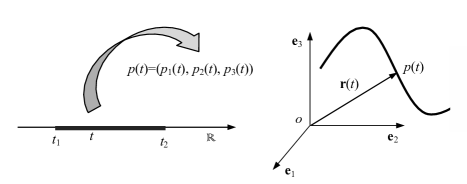
Figure 4.1: Mapping of a curve of points.

The vector function $\mathbf{r}(t)=p(t)-o$ is the position vector of point $p$ in $\mathcal{R}$; the equation

$$\mathbf{r}(t)=r_{i}(t)\mathbf{e}_{i}=r_{1}(t)\mathbf{e}_{1}+r_{2}(t)\mathbf{e}_{2}+r_{3}(t)\mathbf{e}_{3}\ \rightarrow\ \left\{\begin{array}[]{l}r_{1}=r_{1}(t)\\ r_{2}=r_{2}(t)\\ r_{3}=r_{3}(t)\end{array}\right.$$

is the parametric vector equation of the curve: To each value of $t\in[t_{1},t_{2}]$ there corresponds a vector of $\mathcal{V}$ that determines a point of the curve in $\mathcal{E}$ through the operation $p(t)=o+\mathbf{r}(t)$.

Similarly, if the components $L_{ij}(t)$ are continuous functions of a parameter $t$, the mapping $\mathbf{L}(t):[t_{1},t_{2}]\rightarrow Lin(\mathcal{V})$ defined by

$$\mathbf{L}(t)=L_{ij}(t)\mathbf{e}_{i}\otimes\mathbf{e}_{j},\ \ i,j=1,2,3,$$

is a curve of tensors. In the same way we can give a curve of fourth-rank tensors $\mathbb{L}(t):[t_{1},t_{2}]\rightarrow\mathbb{L}$in$(\mathcal{V})$ by

$$\mathbb{L}(t)=L_{ijkl}(t)\mathbf{e}_{i}\otimes\mathbf{e}_{j}\otimes\mathbf{e}_{k}\otimes\mathbf{e}_{l},\ \ i,j,k,l=1,2,3.$$

It is worth noting that the choice of the parameter is not unique: The equation $p=p[\tau(t)]$ still represents the same curve $p=p(t)$, through the change of parameter $\tau=\tau(t)$.

The definition given above for the derivative of a curve of points $p=p(t)$ in $t=t_{0}$ is equivalent to the following one (probably more familiar to the reader)

$$\frac{dp(t)}{dt}=\lim_{\varepsilon\rightarrow 0}\frac{p(t_{0}+\varepsilon)-p(t_{0})}{\varepsilon},$$

represented in Fig. 4.2, where it is apparent that $\mathbf{r}^{\prime}(t)=\dfrac{dp(t)}{dt}$ is a vector.

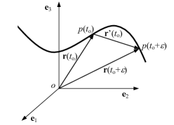
Figure 4.2: Derivative of a curve.

An important case is that of a vector $\mathbf{v}(t)$ whose norm $v(t)$ is constant $\forall t$:

$$(v^{2})^{\prime}=(\mathbf{v}\cdot\mathbf{v})^{\prime}=\mathbf{v}^{\prime}\cdot\mathbf{v}+\mathbf{v}\cdot\mathbf{v}^{\prime}=2\mathbf{v}^{\prime}\cdot\mathbf{v}=0:$$ (4.1)

the derivative of such a vector is orthogonal to it $\forall t$. The contrary is also true, as is immediately apparent.

Finally, using the above rules and assuming that the reference frame $\mathcal{R}$ is independent of $t$, we get easily that

$$\begin{split}&p^{\prime}(t)=p^{\prime}_{i}(t)\ \mathbf{e}_{i},\\ &\mathbf{v}^{\prime}(t)=v^{\prime}_{i}(t)\ \mathbf{e}_{i},\\ &\mathbf{L}^{\prime}(t)=L^{\prime}_{ij}(t)\ \mathbf{e}_{i}\otimes\mathbf{e}_{j},\\ &\mathbb{L}^{\prime}(t)=L^{\prime}_{ijkl}(t)\ \mathbf{e}_{i}\otimes\mathbf{e}_{j}\otimes\mathbf{e}_{k}\otimes\mathbf{e}_{l},\end{split}$$ (4.2)

i.e., the derivative of a curve of points, vectors or tensors is simply calculated differentiating the coordinates of the components. Using this result, it is immediate to prove that

$$\begin{array}[]{c}(\mathbf{L}^{\top})^{\prime}={\mathbf{L}}^{\prime\top},\vskip 6.0pt plus 2.0pt minus 2.0pt\\ (\mathbb{L}^{\top})^{\prime}={\mathbb{L}}^{\prime\top},\end{array}$$

while for any invertible tensor $\mathbf{L}$ it is (we state the following results without proof.)

$$\begin{array}[]{c}(\mathbf{L}^{-1})^{\prime}=-\mathbf{L}^{-1}\mathbf{L}^{\prime}\mathbf{L}^{-1},\vskip 6.0pt plus 2.0pt minus 2.0pt\\ (\det\mathbf{L})^{\prime}=\det\mathbf{L}\ \mathrm{tr}(\mathbf{L}^{\prime}\mathbf{L}^{-1})=\det\mathbf{L}\ {\mathbf{L}^{\top}}^{\prime}\cdot\mathbf{L}^{-1}=\det\mathbf{L}\ \mathbf{L}^{\prime}\cdot\mathbf{L}^{-\top}.\end{array}$$

Let $\mathbf{Q}(t):\mathbb{R}\rightarrow Orth(\mathcal{V})^{+}$ a differentiable function. We call spin tensor the tensor $\mathbf{S}(t)$ defined as

$$\mathbf{S}(t):=\mathbf{Q}^{\prime}(t)\mathbf{Q}^{\top}(t).$$

Then, we have the following

Theorem 24.

(Characterization of the spin tensor). $\mathbf{S}(t)\in Skw(\mathcal{V})\ \forall t\in\mathbb{R}$.

Proof.

As $\mathbf{Q}(t)\in Orth(\mathcal{V})^{+}\ \forall t$, then

$$\mathbf{Q}\mathbf{Q}^{\top}=\mathbf{I}\Rightarrow(\mathbf{Q}\mathbf{Q}^{\top})^{\prime}=\mathbf{Q}^{\prime}\mathbf{Q}^{\top}+\mathbf{Q}{\mathbf{Q}^{\top}}^{\prime}=\mathbf{I}^{\prime}=\mathbf{O}\\ \Rightarrow\mathbf{Q}{\mathbf{Q}^{\top}}^{\prime}=-\mathbf{Q}^{\prime}\mathbf{Q}^{\top}$$

so

$$\mathbf{S}^{\top}=(\mathbf{Q}^{\prime}\mathbf{Q}^{\top})^{\top}=\mathbf{Q}{\mathbf{Q}^{\top}}^{\prime}=-\mathbf{Q}^{\prime}\mathbf{Q}^{\top}=-\mathbf{S}.$$

∎

4.3 Integral of a curve of vectors and length of a curve

We define integral of a curve of vectors $\mathbf{r}(t)$ between $a$ and $b\in[t_{1},t_{2}]$ the curve that is obtained by integrating each component of the curve:

$$\begin{split}&\int_{a}^{b}\mathbf{r}(t)\ dt=\int_{a}^{b}r_{i}(t)\ dt\ \mathbf{e}_{i}.\end{split}$$

If the curve is regular, we can generalize the second fundamental theorem of the integral calculus

$$\mathbf{r}(t)=\mathbf{r}(a)+\int_{a}^{t}\mathbf{r}^{\prime}(t^{*})\ dt^{*}.$$

Because

$$\mathbf{r}(t)=p(t)-o,\ \ \ \mathbf{r}^{\prime}(t)=(p(t)-o)^{\prime}=p^{\prime}(t),$$

we also get

$$p(t)=p(a)+\int_{a}^{t}p^{\prime}(t^{*})\ dt^{*}.$$

The integral of a vector function is the generalization of the vector sum, see Fig. 4.3.

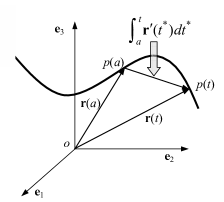
Figure 4.3: Integral of a vector curve.

Let $\mathbf{r}(t):[a,b]\rightarrow\mathcal{E}$ be a regular curve, $\sigma$ a partition of $[a,b]$ of the type $a=t_{0}<t_{1}<...<t_{n}=b$, and

$$\sigma_{max}={\max_{i=1,...,n}}|t_{i}-t_{i-1}|.$$

The length $\ell_{\sigma}$ of the polygonal line whose vertices are the points $\mathbf{r}(t_{i})$ is hence:

$$\ell_{\sigma}=\sum_{i=1}^{n}{|\mathbf{r}(t_{i})-\mathbf{r}(t_{i-1})|}.$$

We define length of the curve $\mathbf{r}(t)$ the (positive) number

$$\ell:=\sup_{\sigma}\ell_{\sigma}.$$

Theorem 25.

Let $\mathbf{r}(t):[a,b]\Rightarrow\mathcal{E}$ be a regular curve, then

$$\ell=\int_{a}^{b}|\mathbf{r}^{\prime}(t)|dt.$$

Proof.

By the fundamental theorem of calculus,

$$\mathbf{r}(t_{i})-\mathbf{r}(t_{i-1})=\int_{t_{i-1}}^{t_{i}}\mathbf{r}^{\prime}(t)dt,$$

so that, using Minkowski’s inequality,

$$|\mathbf{r}(t_{i})-\mathbf{r}(t_{i-1})|=\left|\int_{t_{i-1}}^{t_{i}}\mathbf{r}^{\prime}(t)dt\right|\leq\int_{t_{i-1}}^{t_{i}}|\mathbf{r}^{\prime}(t)|dt,$$

whence

$$\ell\leq\int_{a}^{b}|\mathbf{r}^{\prime}(t)|dt.$$ (4.3)

Because $\mathbf{r}^{\prime}(t)$ is continuous on $[a,b]$, $\forall\varepsilon>0\ \exists\delta>0$ such that $|t-\overline{t}|<\delta\Rightarrow|\mathbf{r}^{\prime}({t})-\mathbf{r}^{\prime}(\overline{t})|<\varepsilon$. Let $t\in[t_{i-1},t_{i}]$ and $\sigma_{max}<\delta$, which is always possible by the choice of the partition $\sigma$; again by the Minkowski’s inequality,

$$|\mathbf{r}^{\prime}(t)|\leq|\mathbf{r}^{\prime}(t)-\mathbf{r}^{\prime}(t_{i})|+|\mathbf{r}^{\prime}(t_{i})|<\varepsilon+|\mathbf{r}^{\prime}(t_{i})|,$$

whence

$$\begin{split}\int_{t_{i-1}}^{t_{i}}|\mathbf{r}^{\prime}(t)|dt&<\int_{t_{i-1}}^{t_{i}}|\mathbf{r}^{\prime}(t_{i})|dt+\varepsilon(t_{i}-t_{i-1})=\left|\int_{t_{i-1}}^{t_{i}}\mathbf{r}^{\prime}(t_{i})dt\right|+\varepsilon(t_{i}-t_{i-1})\\ &\leq\left|\int_{t_{i-1}}^{t_{i}}\mathbf{r}^{\prime}(t)dt\right|+\left|\int_{t_{i-1}}^{t_{i}}(\mathbf{r}^{\prime}(t_{i})-\mathbf{r}^{\prime}(t))dt\right|+\varepsilon(t_{i}-t_{i-1})\\ &\leq|\mathbf{r}(t_{i})-\mathbf{r}(t_{i-1})|+2\varepsilon(t_{i}-t_{i-1}).\end{split}$$

Summing up over all the intervals $[t_{i-1},t_{i}]$ we get

$$\int_{a}^{b}|\mathbf{r}^{\prime}(t)|dt\leq\ell_{\sigma}+2\varepsilon(b-a)\leq\ell+2\varepsilon(b-a),$$

and because $\varepsilon$ is arbitrary,

$$\int_{a}^{b}|\mathbf{r}^{\prime}(t)|dt\leq\ell,$$

which by Eq. (4.3) implies the thesis. ∎

Let $t=f(\tau):[c,d]\rightarrow[a,b]$ be a bijective function that operates the change of parameter from $t$ to $\tau$. If $\mathbf{r}_{t}(t):[a,b]\rightarrow\mathcal{V}$ is a parametric equation of a curve, $\mathbf{r}_{\tau}:[c,d]\rightarrow\mathcal{V}$ is a re-parameterization of the same curve. We then have the following

Theorem 26.

The length of a curve does not depend upon its parameterization.

Proof.

Let $\mathbf{r}_{t}(t):[a,b]\rightarrow\mathcal{E}$ be a regular curve and $t=f(\tau):[c,d]\rightarrow[a,b]$ be a change of parameter; then $dt=f^{\prime}(\tau)d\tau$ and

$$\ell=\int_{a}^{b}|\mathbf{r}_{t}^{\prime}(t)|dt=\int_{c}^{d}|\mathbf{r}_{t}^{\prime}(f(\tau))f^{\prime}(\tau)|d\tau=\int_{c}^{d}|\mathbf{r}_{\tau}^{\prime}(\tau)|d\tau.$$

∎

A simple way to determine a point $p(t)$ on a curve is to fix a point $p_{0}$ on the curve and to measure the length $s(t)$ of the arc of curve between $p_{0}=p(t=0)$ and $p(t)$. This length $s(t)$ is called curvilinear abscissa:

$$s(t)=\int_{0}^{t}|\mathbf{r}^{\prime}(t^{*})|dt^{*}=\int_{0}^{t}|(p(t^{*})-o)^{\prime}|dt^{*}.$$ (4.4)

From Eq. (4.4) we get

$$\frac{ds}{dt}=|\mathbf{r}^{\prime}(t)|>0,$$

so that $s(t)$ is an increasing function of $t$ and the length of an infinitesimal arc is

$$ds=\sqrt{dr_{1}^{2}+dr_{2}^{2}+dr_{3}^{2}}.$$

For a plane curve $y=f(x)$, we can always put $t=x$, which gives the parametric equation

$$p(t)=(t,f(t)),$$

or in vector form

$$\mathbf{r}(t)=t\ \mathbf{e}_{1}+f(t)\ \mathbf{e}_{2},$$

from which we obtain

$$\frac{ds}{dt}=|\mathbf{r}^{\prime}(t)|=|p^{\prime}(t)|=\sqrt{1+f^{\prime 2}(t)},$$ (4.5)

which gives the length of a plane curve between $t=x_{0}$ and $t=x$ as a function of the abscissa $x$:

$$s(x)=\int_{x_{0}}^{x}\sqrt{1+f^{\prime 2}(t)}dt.$$

4.4 The Frenet-Serret basis

We define the tangent vector $\boldsymbol{\tau}(t)$ to a regular curve $p=p(t)$ as the vector

$$\boldsymbol{\tau}(t):=\dfrac{p^{\prime}(t)}{|p^{\prime}(t)|}.$$

By the definition of the derivative, this unit vector is always oriented as the increasing values of $t$; hence, the straight line tangent to the curve in $p_{0}=p(t_{0})$ has the equation

$$q(\bar{t})=p(t_{0})+\bar{t}\ \boldsymbol{\tau}(t_{0}).$$

If the curvilinear abscissa $s$ is chosen as parameter for the curve, through the change of parameter $s=s(t)$ we get

$$\boldsymbol{\tau}(t)=\dfrac{p^{\prime}(t)}{|p^{\prime}(t)|}=\dfrac{p^{\prime}[s(t)]}{|p^{\prime}[s(t)]|}=\frac{1}{s^{\prime}(t)}\frac{dp(s)}{ds}\frac{ds(t)}{dt}=\frac{dp(s)}{ds}\ \rightarrow\boldsymbol{\tau}(s)=p^{\prime}(s).$$ (4.6)

So, if the parameter of the curve is $s$, the derivative of the curve is $\boldsymbol{\tau}$, i.e. it is automatically a unit vector. The above equation, in addition, shows that the change of parameter does not change the direction of the tangent, because it is only a scalar, the derivative of the parameter’s change, that multiplies the vector. Nevertheless, generally speaking, a change of parameter can change the orientation of the curve.

Because the norm of $\boldsymbol{\tau}$ is constant, its derivative is a vector orthogonal to $\boldsymbol{\tau}$, see Eq. (4.1). That is why we call principal normal vector to a curve the unit vector

$$\boldsymbol{\nu}(t):=\frac{\boldsymbol{\tau}^{\prime}(t)}{|\boldsymbol{\tau}^{\prime}(t)|}.$$ (4.7)

$\boldsymbol{\nu}$ is defined only on the points of the curve where $\boldsymbol{\tau}^{\prime}\neq\mathbf{o}$, which implies that $\boldsymbol{\nu}$ is not defined on the points of a straight line. This simply means that there is not, among the infinite unit normal vectors to a straight line, a normal with special properties, a principal one, linked to $\boldsymbol{\tau}$ in a unique way.

Unlike $\boldsymbol{\tau}$, whose orientation changes with the choice of the parameter, $\boldsymbol{\nu}$ is an intrinsic local characteristic of the curve: It is not affected by the choice of the parameter. In fact, by its same definition, $\boldsymbol{\nu}$ does not depend upon the reference frame; then, because the direction of $\boldsymbol{\tau}$ is also independent upon the parameter’s choice, the only factor that could affect $\boldsymbol{\nu}$ is the orientation of the curve, which depends upon the parameter. But a change in the orientation affects, in (4.7), both $\boldsymbol{\tau}$ and the sign of the increment $dt$, so that $\boldsymbol{\tau}^{\prime}(t)=d\boldsymbol{\tau}/dt$ does not change, nor does $\boldsymbol{\nu}$, which is hence an intrinsic property of the curve.

The vector

$$\boldsymbol{\beta}(t):=\boldsymbol{\tau}(t)\times\boldsymbol{\nu}(t)$$

is called the binormal vector; by construction, it is orthogonal to $\boldsymbol{\tau}$ and $\boldsymbol{\nu}$ and it is a unit vector. In addition, it is evident that

$$\boldsymbol{\tau}\times\boldsymbol{\nu}\cdot\boldsymbol{\beta}=1,$$

so the set $\{\boldsymbol{\tau},\boldsymbol{\nu},\boldsymbol{\beta}\}$ forms a positively oriented othonormal basis that can be defined at any regular point of a curve with $\boldsymbol{\tau}^{\prime}\neq\mathbf{o}$. Such a basis is called the Frenet-Serret local basis, local in the sense that it changes with the position along the curve. The plane $(\boldsymbol{\tau},\boldsymbol{\nu})$ is the osculating plane, the plane $(\boldsymbol{\nu},\boldsymbol{\beta})$ the normal plane and the plane $(\boldsymbol{\beta},\boldsymbol{\tau})$ the rectifying plane, see Fig. 4.4.

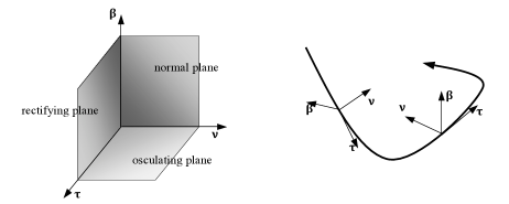
Figure 4.4: The Frenet-Serret basis.

The osculating plane is particularly important: If we consider a plane passing through three nonaligned points of the curve, when these points become closer and closer, still remaining on the curve, the plane tends to the osculating plane: The osculating plane at a point of a curve is hence the plane that better approaches the curve near the point. A plane curve is entirely contained in the osculating plane, which is fixed.

The principal normal $\boldsymbol{\nu}$ is always oriented toward the part of the space, with respect to the rectifying plane, where the curve is; in particular, for a plane curve, $\boldsymbol{\nu}$ is always directed toward the concavity of the curve. To show that, it is sufficient to prove that the vector $p(t+\varepsilon)-p(t)$ forms with $\boldsymbol{\nu}$ an angle $\psi\leq\pi/2$, i.e. that $(p(t+\varepsilon)-p(t))\cdot\boldsymbol{\nu}\geq 0$. In fact,

$$\begin{split}&p(t+\varepsilon)-p(t)=\varepsilon\ p^{\prime}(t)+\frac{1}{2}\varepsilon^{2}p^{\prime\prime}(t)+o(\varepsilon^{2})\ \Rightarrow\\ &(p(t+\varepsilon)-p(t))\cdot\boldsymbol{\nu}=\frac{1}{2}\varepsilon^{2}p^{\prime\prime}(t)\cdot\boldsymbol{\nu}+o(\varepsilon^{2}),\end{split}$$

but

$$p^{\prime\prime}(t)\cdot\boldsymbol{\nu}=(\boldsymbol{\tau}^{\prime}|p^{\prime}|+\boldsymbol{\tau}|p^{\prime}|^{\prime})\cdot\boldsymbol{\nu}=(|\boldsymbol{\tau}^{\prime}||p^{\prime}|\boldsymbol{\nu}+\boldsymbol{\tau}|p^{\prime}|^{\prime})\cdot\boldsymbol{\nu}=|\boldsymbol{\tau}^{\prime}||p^{\prime}|,$$

so that, to within infinitesimal quantities of order $o(\varepsilon^{2})$, we obtain

$$(p(t+\varepsilon)-p(t))\cdot\boldsymbol{\nu}=\frac{1}{2}\varepsilon^{2}|\boldsymbol{\tau}^{\prime}||p^{\prime}|\geq 0.$$

4.5 Curvature of a curve

It is important, in several situations, to evaluate how much a curve moves away from a straight line, in the neighborhood of a point. To do that, we calculate the angle formed by the tangents at two close points, determined by the curvilinear abscissae $s$ and $s+\varepsilon$, and we measure the angle $\chi(s,\varepsilon)$ that they form, see Fig. 4.5.

Figure 4.5: Curvature of a curve.

We then define curvature of the curve in $p=p(s)$ as the limit

$$c(s)=\lim_{\varepsilon\rightarrow 0}\left|\frac{\chi(s,\varepsilon)}{\varepsilon}\right|.$$

The curvature is hence a non-negative scalar that measures the rapidity of variation in the direction of the curve per unit length of the curve (that is why $c(s)$ is defined as a function of the curvilinear abscissa); by its same definition, the curvature is an intrinsic property of the curve, i.e. independent of the parameter’s choice. For a straight line, the curvature is everywhere identically null.

The curvature is linked to the second derivative of the curve; referring to Fig. 4.5, it is

$$\begin{split}c(s)&=\lim_{\varepsilon\rightarrow 0}\left|\frac{\chi(s,\varepsilon)}{\varepsilon}\right|=\lim_{\varepsilon\rightarrow 0}\left|\frac{\sin\chi(s,\varepsilon)}{\varepsilon}\right|=\lim_{\varepsilon\rightarrow 0}\left|\frac{2}{\varepsilon}\sin\frac{\chi(s,\varepsilon)}{2}\right|\\ &=\lim_{\varepsilon\rightarrow 0}\left|\frac{\mathbf{v}(s,\varepsilon)}{\varepsilon}\right|=\lim_{\varepsilon\rightarrow 0}\left|\frac{\boldsymbol{\tau}(s+\varepsilon)-\boldsymbol{\tau}(s)}{\varepsilon}\right|=|\boldsymbol{\tau}^{\prime}(s)|=|p^{\prime\prime}(s)|.\end{split}$$

Another formula for the calculation of $c(s)$ can be obtained if we consider that

$$\frac{d\boldsymbol{\tau}[s(t)]}{dt}=\frac{d\boldsymbol{\tau}}{ds}\frac{ds}{dt}=\frac{d\boldsymbol{\tau}}{ds}|p^{\prime}(t)|\ \rightarrow\ \frac{d\boldsymbol{\tau}}{ds}=\frac{1}{|p^{\prime}(t)|}\frac{d\boldsymbol{\tau}}{dt},$$

so that

$$c(s)=|\boldsymbol{\tau}^{\prime}(s)|=\frac{1}{|p^{\prime}(t)|}\left|\frac{d\boldsymbol{\tau}}{dt}\right|=\frac{|\boldsymbol{\tau}^{\prime}(t)|}{|p^{\prime}(t)|}.$$ (4.8)

A better formula can be obtained using the complementary projector onto $\boldsymbol{\tau}$, i.e. the tensor $\mathbf{I}-\boldsymbol{\tau}\otimes\boldsymbol{\tau}$, introduced in Exercise 2.2:

$$\begin{split}\frac{d\boldsymbol{\tau}}{ds}&=\frac{1}{|p^{\prime}(t)|}\frac{d\boldsymbol{\tau}}{dt}=\frac{1}{|p^{\prime}(t)|}\frac{d}{dt}\frac{p^{\prime}(t)}{|p^{\prime}(t)|}=\frac{1}{|p^{\prime}|}\frac{p^{\prime\prime}|p^{\prime}|-p^{\prime}\dfrac{p^{\prime\prime}\cdot p^{\prime}}{|p^{\prime}|}}{|p^{\prime}|^{2}}\\ &=\frac{p^{\prime\prime}-\boldsymbol{\tau}\ p^{\prime\prime}\cdot\boldsymbol{\tau}}{|p^{\prime}|^{2}}=(\mathbf{I}-\boldsymbol{\tau}\otimes\boldsymbol{\tau})\frac{p^{\prime\prime}}{|p^{\prime}|^{2}}.\end{split}$$

Consequently,

$$c(s)=\left|\frac{d\boldsymbol{\tau}(s)}{ds}\right|=\frac{1}{|p^{\prime}|^{2}}|(\mathbf{I}-\boldsymbol{\tau}\otimes\boldsymbol{\tau})p^{\prime\prime}|.$$

Now, we use Eq. (2.36) with $\mathbf{w}=\boldsymbol{\tau}$; denoting by $\mathbf{W}_{\tau}$ the axial tensor of $\boldsymbol{\tau}$, then

$$\mathbf{W}_{\tau}\mathbf{W}_{\tau}=-\frac{1}{2}|\mathbf{W}_{\tau}|^{2}(\mathbf{I}-\boldsymbol{\tau}\otimes\boldsymbol{\tau}),$$

whence

$$\mathbf{I}-\boldsymbol{\tau}\otimes\boldsymbol{\tau}=-2\frac{\mathbf{W}_{\tau}\mathbf{W}_{\tau}}{|\mathbf{W}_{\tau}|^{2}}=-\mathbf{W}_{\tau}\mathbf{W}_{\tau},$$

because if $\boldsymbol{\tau}=(\tau_{1},\tau_{2},\tau_{3})$, then

$$\begin{split}|\mathbf{W}_{\tau}|^{2}&=\mathbf{W}_{\tau}\cdot\mathbf{W}_{\tau}=\left[\begin{array}[]{ccc}0&-\tau_{3}&\tau_{2}\\ \tau_{3}&0&-\tau_{1}\\ -\tau_{2}&\tau_{1}&0\end{array}\right]\cdot\left[\begin{array}[]{ccc}0&-\tau_{3}&\tau_{2}\\ \tau_{3}&0&-\tau_{1}\\ -\tau_{2}&\tau_{1}&0\end{array}\right]\\ &=2(\tau_{1}^{2}+\tau_{2}^{2}+\tau_{3}^{2})=2.\end{split}$$

So, because $\mathbf{W}_{\tau}\in Skw(\mathcal{V})$,

$$\mathbf{W}_{\tau}\ \mathbf{u}=\boldsymbol{\tau}\times\mathbf{u}\ \ \forall\mathbf{u}\in\mathcal{V}.$$

Finally, using Eq. (2.29), the orthogonality property of cross product, Eq. (2.27) and Eq. (2.31), we get

$$\begin{split}|(\mathbf{I}-\boldsymbol{\tau}\otimes\boldsymbol{\tau})p^{\prime\prime}|&=|-\mathbf{W}_{\tau}\mathbf{W}_{\tau}p^{\prime\prime}|=|-\mathbf{W}_{\tau}(\boldsymbol{\tau}\times p^{\prime\prime})|=|-\boldsymbol{\tau}\times(\boldsymbol{\tau}\times p^{\prime\prime})|\\ &=|\boldsymbol{\tau}\times(\boldsymbol{\tau}\times p^{\prime\prime})|=|\boldsymbol{\tau}\times p^{\prime\prime}|=\frac{|p^{\prime}\times p^{\prime\prime}|}{|p^{\prime}|},\end{split}$$

so that, finally,

$$c=\frac{|p^{\prime}\times p^{\prime\prime}|}{|p^{\prime}|^{3}}.$$ (4.9)

Applying this last formula to a plane curve $p(t)=(x(t),y(t))$, we get

$$c=\frac{|x^{\prime}y^{\prime\prime}-x^{\prime\prime}y^{\prime}|}{(x^{\prime 2}+y^{\prime 2})^{\frac{3}{2}}},$$

and if the curve is given in the form $y=y(x)$, so that the parameter $t=x$, then we obtain

$$c=\frac{|y^{\prime\prime}|}{(1+y^{\prime 2})^{\frac{3}{2}}}.$$

This last formula shows that if $|y^{\prime}|\ll 1$, then

$$c\simeq|y^{\prime\prime}|.$$

This result is fundamental in the linearized (infinitesimal) theory of beams, plates and shells.

4.6 The Frenet-Serret formulae

From Eq. (4.7) for $t=s$ and Eq. (4.8), we get

$$\frac{d\boldsymbol{\tau}}{ds}=c\ \boldsymbol{\nu}$$ (4.10)

which is the first Frenet-Serret Formula, giving the variation in $\boldsymbol{\tau}$ per unit length of the curve. Such a variation is a vector whose norm is the curvature and the direction is that of $\boldsymbol{\nu}$. We remark that, because $t=s$, by Eq. (4.6) it is also

$$p^{\prime\prime}(s)=c(s)\boldsymbol{\nu}(s).$$ (4.11)

Let us now consider the variation in $\boldsymbol{\beta}$ per unit length of the curve; because $\boldsymbol{\beta}$ is a unit vector, we have

$$\frac{d\boldsymbol{\beta}}{ds}\cdot\boldsymbol{\beta}=0,$$

and

$$\boldsymbol{\beta}\cdot\boldsymbol{\tau}=0\ \Rightarrow\ \frac{d(\boldsymbol{\beta}\cdot\boldsymbol{\tau})}{ds}=\frac{d\boldsymbol{\beta}}{ds}\cdot\boldsymbol{\tau}+\boldsymbol{\beta}\cdot\frac{d\boldsymbol{\tau}}{ds}=0.$$

Through Eq. (4.10) and because $\boldsymbol{\beta}\cdot\boldsymbol{\nu}=0$ we get

$$\frac{d\boldsymbol{\beta}}{ds}\cdot\boldsymbol{\tau}=-c\ \boldsymbol{\beta}\cdot\boldsymbol{\nu}=0,$$

so that $\dfrac{d\boldsymbol{\beta}}{ds}$ is necessarily parallel to $\boldsymbol{\nu}$. We then set

$$\frac{d\boldsymbol{\beta}}{ds}=\vartheta\boldsymbol{\nu},$$

which is the second Frenet-Serret formula. The scalar $\vartheta(s)$ is called the torsion of the curve in $p=p(s)$. So, we see that the variation in $\boldsymbol{\beta}$ per unit length is a vector parallel to $\boldsymbol{\nu}$ and proportional to the torsion of the curve.

We can now find the variation in $\boldsymbol{\nu}$ per unit length of the curve:

$$\frac{d\boldsymbol{\nu}}{ds}=\frac{d(\boldsymbol{\beta}\times\boldsymbol{\tau})}{ds}=\frac{d\boldsymbol{\beta}}{ds}\times\boldsymbol{\tau}+\boldsymbol{\beta}\times\frac{d\boldsymbol{\tau}}{ds}=\vartheta\ \boldsymbol{\nu}\times\boldsymbol{\tau}+c\ \boldsymbol{\beta}\times\boldsymbol{\nu},$$

so finally

$$\frac{d\boldsymbol{\nu}}{ds}=-c\ \boldsymbol{\tau}-\vartheta\ \boldsymbol{\beta},$$

which is the third Frenet-Serret formula: The variation in $\boldsymbol{\nu}$ per unit length of the curve is a vector of the rectifying plane.

The three formulae of Frenet-Serret (discovered independently by J. F. Frenet in 1847 and by J. A. Serret in 1851) can be condensed in the symbolic matrix product

$$\left\{\begin{array}[]{c}\boldsymbol{\tau}^{\prime}\\ \boldsymbol{\nu}^{\prime}\\ \boldsymbol{\beta}^{\prime}\end{array}\right\}=\left[\begin{array}[]{ccc}0&c&0\\ -c&0&-\vartheta\\ 0&\vartheta&0\end{array}\right]\left\{\begin{array}[]{c}\boldsymbol{\tau}\\ \boldsymbol{\nu}\\ \boldsymbol{\beta}\end{array}\right\}.$$

The matrix in the equation above is called the matrix of Cartan, and it is skew.

4.7 The torsion of a curve

We have introduced the torsion of a curve in the previous section, with the second formula of Frenet-Serret. The torsion measures the deviation of a curve from flatness: If a curve is planar, it belongs to the osculating plane and $\boldsymbol{\beta}$, which is perpendicular to the osculating pane, is hence a constant vector. So, its derivative is null, and by the Frenet-Serret second formula, $\vartheta=0$.

Conversely, if $\vartheta=0$ everywhere, $\boldsymbol{\beta}$ is a constant vector and hence the osculating plane does not change and the curve is planar. So we have that a curve is planar if and only if the torsion is null $\forall p(s)$.

Using the Frenet-Serret formulae in the expression of $p^{\prime\prime\prime}(s)$, we get a formula for the torsion:

$$\begin{split}&p^{\prime}(t)=|p^{\prime}|\boldsymbol{\tau}=\frac{dp}{ds}\frac{ds}{dt}=s^{\prime}\boldsymbol{\tau}\ \Rightarrow\ |p^{\prime}|=s^{\prime}\ \rightarrow\\ &p^{\prime\prime}(t)=s^{\prime\prime}\boldsymbol{\tau}+s^{\prime}\boldsymbol{\tau}^{\prime}=s^{\prime\prime}\boldsymbol{\tau}+s^{\prime 2}\frac{d\boldsymbol{\tau}}{ds}=s^{\prime\prime}\boldsymbol{\tau}+c\ s^{\prime 2}\boldsymbol{\nu}\ \rightarrow\\ &p^{\prime\prime\prime}(t)=s^{\prime\prime\prime}\boldsymbol{\tau}+s^{\prime\prime}\boldsymbol{\tau}^{\prime}+(c\ s^{\prime 2})^{\prime}\boldsymbol{\nu}+c\ s^{\prime 2}\boldsymbol{\nu}^{\prime}\\ &\hskip 27.0301pt=s^{\prime\prime\prime}\boldsymbol{\tau}+s^{\prime\prime}s^{\prime}\frac{d\boldsymbol{\tau}}{ds}+(c\ s^{\prime 2})^{\prime}\boldsymbol{\nu}+c\ s^{\prime 3}\frac{d\boldsymbol{\nu}}{ds}\\ &\hskip 27.0301pt=s^{\prime\prime\prime}\boldsymbol{\tau}+s^{\prime\prime}s^{\prime}c\boldsymbol{\nu}+(c\ s^{\prime 2})^{\prime}\boldsymbol{\nu}-c\ s^{\prime 3}(c\boldsymbol{\tau}+\vartheta\boldsymbol{\beta})\\ &\hskip 27.0301pt=(s^{\prime\prime\prime}-c^{2}s^{\prime 3})\boldsymbol{\tau}+(s^{\prime\prime}s^{\prime}c+c^{\prime}s^{\prime 2}+2c\ s^{\prime}s^{\prime\prime})\boldsymbol{\nu}-c\ s^{\prime 3}\vartheta\boldsymbol{\beta},\end{split}$$

whence, through Eq. (4.9),

$$\begin{split}p^{\prime}\times p^{\prime\prime}\cdot p^{\prime\prime\prime}&=s^{\prime}\boldsymbol{\tau}\times(s^{\prime\prime}\boldsymbol{\tau}+c\ s^{\prime 2}\boldsymbol{\nu})\cdot[(s^{\prime\prime\prime}-c^{2}s^{\prime 3})\boldsymbol{\tau}\\ &+(s^{\prime\prime}s^{\prime}c+c^{\prime}s^{\prime 2}+2c\ s^{\prime}s^{\prime\prime})\boldsymbol{\nu}-c\ s^{\prime 3}\vartheta\boldsymbol{\beta}]\\ &=-c^{2}s^{\prime 6}\vartheta=-c^{2}|p^{\prime}|^{6}\vartheta=-\frac{|p^{\prime}\times p^{\prime\prime}|^{2}}{|p^{\prime}|^{6}}|p^{\prime}|^{6}\vartheta,\end{split}$$

so that, finally,

$$\vartheta=-\frac{p^{\prime}\times p^{\prime\prime}\cdot p^{\prime\prime\prime}}{|p^{\prime}\times p^{\prime\prime}|^{2}}.$$

We remark that, while the curvature is linked to the second derivative of the curve, the torsion is also a function of the third derivative.

Unlike curvature, which is intrinsically positive, the torsion can be negative. In fact, again using the Frenet-Serret formulae,

$$\begin{split}p(s+\varepsilon)-p(s)&=\varepsilon\ p^{\prime}+\frac{1}{2}\varepsilon^{2}p^{\prime\prime}+\frac{1}{6}\varepsilon^{3}p^{\prime\prime\prime}+o(\varepsilon^{3})\\ &=\varepsilon\boldsymbol{\tau}+\frac{1}{2}\varepsilon^{2}c\boldsymbol{\nu}+\frac{1}{6}\varepsilon^{3}(c\boldsymbol{\nu})^{\prime}+o(\varepsilon^{3})\\ &=\varepsilon\boldsymbol{\tau}+\frac{1}{2}\varepsilon^{2}c\boldsymbol{\nu}+\frac{1}{6}\varepsilon^{3}(c^{\prime}\boldsymbol{\nu}-c^{2}\boldsymbol{\tau}-c\ \vartheta\boldsymbol{\beta})+o(\varepsilon^{3})\\ &\Rightarrow(p(s+\varepsilon)-p(s))\cdot\boldsymbol{\beta}=-\frac{1}{6}\varepsilon^{3}c\ \vartheta+o(\varepsilon^{3}).\end{split}$$

The above dot product determines whether the point $p(s+\varepsilon)$ is located, with respect to the osculating plane, on the side of $\boldsymbol{\beta}$ or on the opposite one, see Fig. 4.6: If following the curve for increasing values of $s,\ \varepsilon>0$, the point passes into the semi-space of $\boldsymbol{\beta}$ from the opposite one, because $1/6\ c\ \varepsilon^{3}>0$, it will be $\vartheta<0$, while in the opposite case it will be $\vartheta>0$.

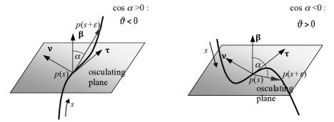
Figure 4.6: Torsion of a curve.

This result is intrinsic, i.e. it does not depend upon the choice of the parameter, hence of the positive orientation of the curve; in fact, $\boldsymbol{\nu}$ is intrinsic, but changing the orientation of the curve, $\boldsymbol{\tau}$, and hence $\boldsymbol{\beta}$, change in orientation.

4.8 Osculating sphere and circle

The osculating sphere to a curve at a point $p$ is a sphere to which the curve tends to adhere in the neighborhood of $p$. Mathematically, if $q_{s}$ is the center of the sphere relative to the point $p(s)$, then

$$|p(s+\varepsilon)-q_{s}|^{2}=|p(s)-q_{s}|^{2}+o(\varepsilon^{3}).$$

Using this definition, discarding the terms of order $o(\varepsilon^{3})$ and using the Frenet-Serret formulae, we get:

$$\begin{split}|p(s+\varepsilon)-q_{s}|^{2}&=|p(s)-q_{s}+\varepsilon p^{\prime}+\frac{1}{2}\varepsilon^{2}p^{\prime\prime}+\frac{1}{6}\varepsilon^{3}p^{\prime\prime\prime}+o(\varepsilon^{3})|^{2}\\ &=|p(s)-q_{s}+\varepsilon\boldsymbol{\tau}+\frac{1}{2}\varepsilon^{2}c\ \boldsymbol{\nu}+\frac{1}{6}\varepsilon^{3}(c\boldsymbol{\nu})^{\prime}+o(\varepsilon^{3})|^{2}\\ &=|p(s)-q_{s}|^{2}+2\varepsilon(p(s)-q_{s})\cdot\boldsymbol{\tau}+\varepsilon^{2}+\varepsilon^{2}c(p(s)-q_{s})\cdot\boldsymbol{\nu}\\ &+\frac{1}{3}\varepsilon^{3}(p(s)-q_{s})\cdot(c^{\prime}\boldsymbol{\nu}-c^{2}\boldsymbol{\tau}-c\ \vartheta\boldsymbol{\beta})+o(\varepsilon^{3}),\end{split}$$

which gives

$$\begin{split}&(p(s)-q_{s})\cdot\boldsymbol{\tau}=0,\\ &(p(s)-q_{s})\cdot\boldsymbol{\nu}=-\frac{1}{c}=-\rho,\\ &(p(s)-q_{s})\cdot\boldsymbol{\beta}=-\frac{c^{\prime}}{c^{2}\vartheta}=\frac{\rho^{\prime}}{\vartheta},\end{split}$$

and finally

$$q_{s}=p+\rho\ \boldsymbol{\nu}-\frac{\rho^{\prime}}{\vartheta}\boldsymbol{\beta},$$ (4.12)

so the center of the sphere belongs to the normal plane; the sphere is not defined for a plane curve. The quantity $\rho$ is the radius of curvature of the curve, defined as

$$\rho=\frac{1}{c}.$$

The radius of the osculating sphere is

$$\rho_{s}=|p-q_{s}|=\sqrt{\rho^{2}+\left(\frac{\rho^{\prime}}{\vartheta}\right)^{2}}.$$

The intersection between the osculating sphere and the osculating plane at a same point $p$ is the osculating circle. This circle has the property of sharing the same tangent in $p$ with the curve and its radius is the radius of curvature, $\rho$. From Eq. (4.12) we get the position of the osculating circle center $q$:

$$q=p+\rho\ \boldsymbol{\nu}.$$ (4.13)

An example can be seen in Fig. 4.7, where the osculating plane, circle and sphere are shown for a point $p$ of a conical helix.

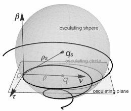
Figure 4.7: Osculating plane, circle and sphere for a point $p$ of a conical helix.

The osculating circle is a diametral circle of the osculating sphere only when $q=q_{s}$, so if and only if

$$\frac{\rho^{\prime}}{\vartheta}=-\frac{c^{\prime}}{c^{2}\vartheta}=0,$$

i.e. when the curvature is constant.

4.9 Evolute, involute and envelopes of plane curves

For any plane curve $\boldsymbol{\gamma}(s)$, the center of the osculating circle $q$ describes a curve $\boldsymbol{\delta}(\sigma)$ that is called the evolute of $\boldsymbol{\gamma}(s)$ ($s$ and $\sigma$ are curvilinear abscissae). A point $q$ of the evolute is then given by Eq. (4.13). We call involute of a curve $\boldsymbol{\gamma}(s)$ a curve $\boldsymbol{\mu}(\sigma)$ whose evolute is $\boldsymbol{\gamma}(s)$. We call envelope of a family of plane curves $\boldsymbol{\varphi}(s,\kappa),\kappa\in\mathbb{R}$ being a parameter, a curve that is tangent, in each of its points, to the curve of $\boldsymbol{\varphi}(s,\kappa)$ passing through that point.

Let us consider the evolute $\boldsymbol{\delta}(\sigma)$ of a curve $\boldsymbol{\gamma}(s)$; the tangent to $\boldsymbol{\delta}(\sigma)$ is the vector, cf. Eq. (4.13),

$$\boldsymbol{\tau}_{\delta}=\frac{dq}{d\sigma}=\frac{dq}{ds}\frac{ds}{d\sigma}.$$

But, cf. again Eq. (4.13) and the Frenet-Serret formulae,

$$\frac{dq}{ds}=\frac{dp}{ds}+\frac{d\rho}{ds}\boldsymbol{\nu}+\rho\frac{d\boldsymbol{\nu}}{ds}=\boldsymbol{\tau}+\frac{d\rho}{ds}\boldsymbol{\nu}-\rho\ c\ \boldsymbol{\tau}=\frac{d\rho}{ds}\boldsymbol{\nu},$$

so

$$\boldsymbol{\tau}_{\delta}=\frac{dq}{d\sigma}=\frac{d\rho}{ds}\frac{ds}{d\sigma}\boldsymbol{\nu}.$$

Because

$$\left|{\frac{dq}{d\sigma}}\right|=|\boldsymbol{\nu}|=1,$$

then

$$\frac{d\rho}{ds}\frac{ds}{d\sigma}=1\ \Rightarrow\ \frac{d\rho}{ds}=\frac{d\sigma}{ds}$$

and

$$\boldsymbol{\tau}_{\delta}=\boldsymbol{\nu}.$$

The evolute, $\boldsymbol{\delta}(\sigma)$, of $\boldsymbol{\gamma}(s)$ is hence the envelope of its principal normals $\boldsymbol{\nu}(s)$.

This result helps us in finding the equation of the involute $\boldsymbol{\mu}(\sigma)$ of a curve $\boldsymbol{\gamma}(s)$; let $p=p(s)$ be a point of $\boldsymbol{\gamma}(s)$; then, if $b\in\boldsymbol{\mu}(\sigma)$, it must be that

$$(b-p)\cdot\boldsymbol{\nu}=0$$

where $\boldsymbol{\nu}$ is the principal normal to $\boldsymbol{\gamma}(s)$ in $p$, because $\boldsymbol{\gamma}(s)$ is the evolute of $\boldsymbol{\mu}(\sigma)$, which implies, for the last result, that $\boldsymbol{\tau}=\boldsymbol{\nu}_{\mu}$, with $\boldsymbol{\tau}$ the tangent to $\boldsymbol{\gamma}(s)$ in $p$ and $\boldsymbol{\nu}_{\mu}$ the principal normal to $\boldsymbol{\mu}(\sigma)$ in $b$, see Fig. 4.8.

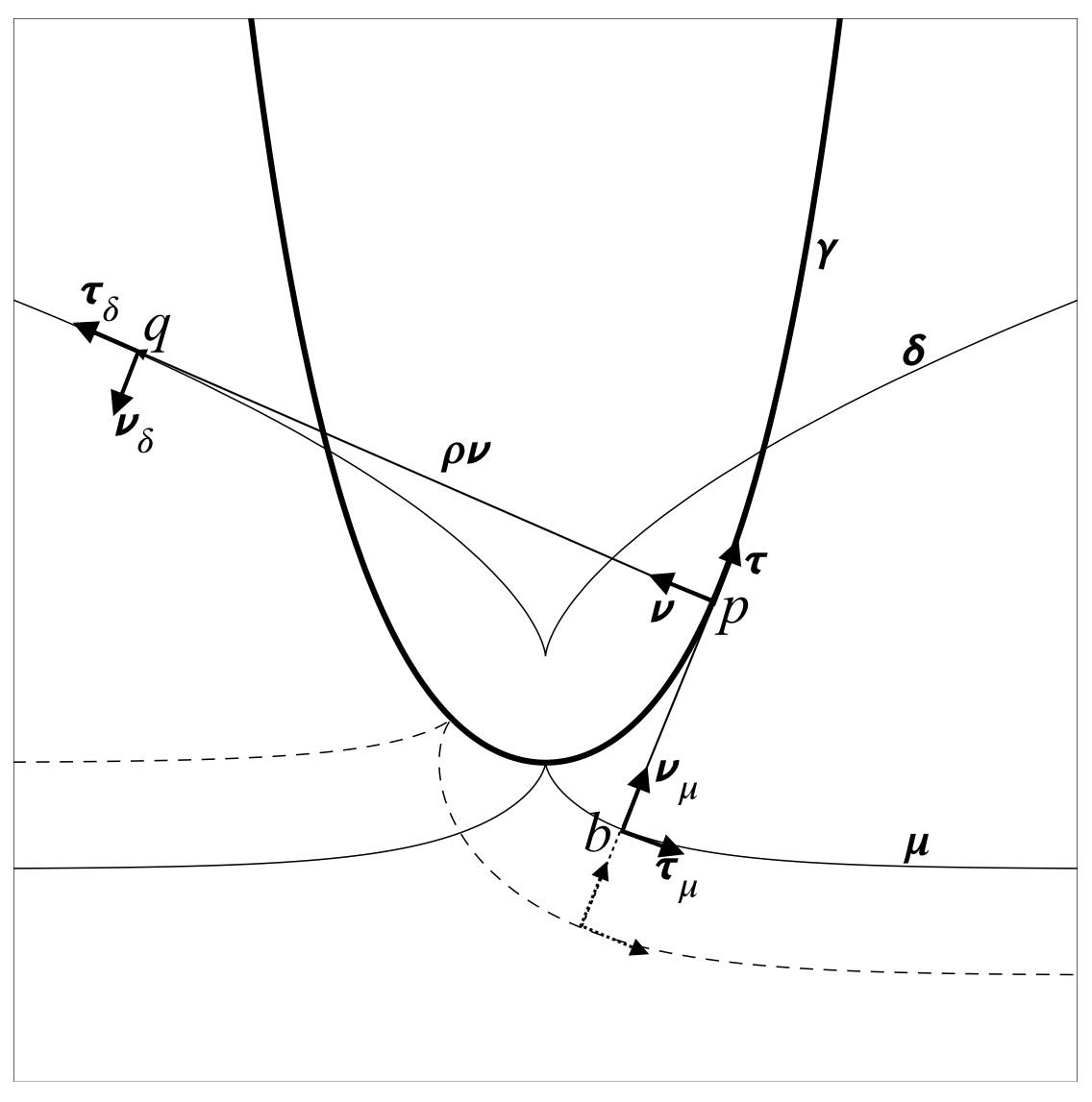
Figure 4.8: Evolute, $\boldsymbol{\delta}$, and involutes for $a=0$, denoted by $\boldsymbol{\mu}$, and $a=1$, dashed, of a catenary $\boldsymbol{\gamma}$.

Therefore,

$$b(s)-p(s)=f(s)\boldsymbol{\tau}(s)\ \rightarrow\ b(s)=p(s)+f(s)\boldsymbol{\tau}(s),$$

with $f=f(s)$ a scalar function of $s$; to remark that $b=b(s)$, i.e. the arc-length $s$ of $\boldsymbol{\gamma}(s)$ is the parameter also for $\boldsymbol{\mu}(s)$, but in general $\sigma\neq s$. Upon differentiation, we get

$$b^{\prime}(s)=(1+f^{\prime}(s))\boldsymbol{\tau}(s)+f(s)c(s)\boldsymbol{\nu}(s).$$

Then, because $b^{\prime}(s)=|b^{\prime}(s)|\boldsymbol{\tau}_{\mu}$ is orthogonal to $\boldsymbol{\nu}_{\mu}=\boldsymbol{\tau}$, it is parallel to $\boldsymbol{\nu}$, so it must be that

$$1+f^{\prime}(s)=0\ \Rightarrow\ f(s)=a-s,\ \ \ a\in\mathbb{R}.$$

Finally, the equation of the involute $\boldsymbol{\mu}(s)$ to $\boldsymbol{\gamma}(s)$ is

$$b(s)=p(s)+(a-s)\boldsymbol{\tau}(s),$$

and we remark that the involute is not unique.

4.10 The theorem of Bonnet

The curvature, $c(s)$, and the torsion, $\vartheta(s)$, are the only differential parameters that completely describe a curve. In other words, given two functions $c(s)$ and $\vartheta(s)$, then a curve exists with such a curvature and torsion (we remark that there are no conditions bounding these parameters). This is proved in the following

Theorem 27.

(Bonnet’s theorem). Given two scalar functions $c(s)\in$C¹ and $\vartheta(s)\in$C⁰, there always exists a unique curve $\boldsymbol{\gamma}\in$C³ whose curvilinear abscissa is $s$, curvature $c(s)$ and torsion $\vartheta(s)$.

Proof.

Let

$$\mathbf{e}=\left(\begin{array}[]{c}\boldsymbol{\tau}\\ \boldsymbol{\nu}\\ \boldsymbol{\beta}\end{array}\right)$$

be the column vector whose elements are the vectors of the Frenet-Serret basis. Then

$$\frac{d\mathbf{e}(s)}{ds}=\mathbf{C}(s)\mathbf{e}(s)$$ (4.14)

with

$$\mathbf{C}(s)=\left[\begin{array}[]{ccc}0&c(s)&0\\ -c(s)&0&-\vartheta(s)\\ 0&\vartheta(s)&0\end{array}\right]$$

the matrix of Cartan. Adding the initial condition

$$\mathbf{e}(0)=\left(\begin{array}[]{c}\mathbf{e}_{1}\\ \mathbf{e}_{2}\\ \mathbf{e}_{3}\end{array}\right)$$

we have a Cauchy problem for the basis $\mathbf{e}(0)$. As known, such a problem admits a unique solution, i.e. we can associate to $c(s)$ and $\vartheta(s)$ a family of bases $\mathbf{e}(s)$ (that are orthonormal because if one of them were not so, the Cartan’s matrix should not be skew). Call $\boldsymbol{\tau}(s)$ the first vector of the basis $\mathbf{e}(s)$ and define the function

$$p(s):=p_{0}+\int_{0}^{s}\boldsymbol{\tau}(s^{*})ds^{*};$$

$p(s)$ is the curve looked for (it depends upon an arbitrary point $p_{0}$, i.e. upon an inessential rigid displacement). In fact, because $|\boldsymbol{\tau}|=1$, $s$ is the curvilinear abscissa of the curve. Then, it is sufficient to write the Frenet-Serret equations identifying them with the system (4.14). ∎

4.11 Canonic equations of a curve

We call the canonic equations of a curve at a point $p_{0}$ the equations of the curve referred to the Frenet-Serret basis in $p_{0}$. For this purpose, we expand the curve in a Taylor series of initial point $p_{0}$:

$$p(s)=p_{0}+s\ p^{\prime}(0)+\frac{1}{2}s^{2}p^{\prime\prime}(0)+\frac{1}{6}s^{3}p^{\prime\prime\prime}(0)+o(s^{3}).$$

In the Frenet-Serret basis,

$$p^{\prime}(0)=\boldsymbol{\tau}(0),\ \ p^{\prime\prime}(0)=c(0)\boldsymbol{\nu}(0),\ \ p^{\prime\prime\prime}(0)=\left.\dfrac{dc\boldsymbol{\nu}}{ds}\right|_{s=0}=c^{\prime}(0)\boldsymbol{\nu}(0)-c^{2}(0)\boldsymbol{\tau}(0)-c(0)\vartheta(0)\boldsymbol{\beta}(0),$$

so

$$p(s)=p_{0}+s\ \boldsymbol{\tau}(0)+\frac{1}{2}s^{2}c(0)\boldsymbol{\nu}(0)+\dfrac{1}{6}s^{3}(-c^{2}(0)\boldsymbol{\tau}(0)+c^{\prime}(0)\boldsymbol{\nu}(0)-c(0)\vartheta(0)\boldsymbol{\beta}(0))+o(s^{3}).$$

The coordinates of a point $p(s)$ close to $p_{0}$, in the basis $\{\boldsymbol{\tau}(0),\boldsymbol{\nu}(0),\boldsymbol{\beta}(0)\}$, are hence

$$\begin{split}&p_{1}(s)=s-\frac{1}{6}c^{2}(0)s^{3}+o(s^{3}),\\ &p_{2}(s)=\frac{1}{2}c(0)s^{2}+\dfrac{1}{6}c^{\prime}(0)s^{3}+o(s^{3}),\\ &p_{3}(s)=-\frac{1}{6}c(0)\vartheta(0)s^{3}+o(s^{3}).\end{split}$$

The projections of the curve onto the planes of the Frenet-Serret basis hence have, close to $p_{0}$ (i.e. retaining the first non null term in the expressions above), the following equations:

• On the osculating plane

  $$\left\{\begin{array}[]{l}p_{1}(s)=s,\\ p_{2}(s)=\dfrac{1}{2}c(0)s^{2},\end{array}\right.$$

  or, eliminating $s$,

  $$p_{2}=\dfrac{1}{2}c(0)p_{1}^{2},$$

  which is the equation of a parabola.

• On the rectifying plane

  $$\left\{\begin{array}[]{l}p_{1}(s)=s,\\ p_{3}(s)=-\dfrac{1}{6}c(0)\vartheta(0)s^{3},\end{array}\right.$$

  or, eliminating $s$,

  $$p_{3}=-\frac{1}{6}c(0)\vartheta(0)p_{1}^{3},$$

  which is the equation of a cubic parabola.

• On the normal plane

  $$\left\{\begin{array}[]{l}p_{2}(s)=\dfrac{1}{2}c(0)s^{2},\\ p_{3}(s)=-\dfrac{1}{6}c(0)\vartheta(0)s^{3},\end{array}\right.$$

  or, eliminating $s$,

  $$p_{3}^{2}=\frac{2}{9}\frac{\vartheta^{2}(0)}{c(0)}p_{2}^{3},$$

  which is the equation of a semicubic parabola, with a cusp at the origin, hence a singular point, though the curve $p(s)$ is regular.

4.12 Exercises

1. Using the same definition of derivative of a curve, prove the relations in Sect. (4.2).

2. Prove the relations in Eq. (4.2).

3. The curve whose polar equation is

   $$r=a\ \theta,\ \ a\in\mathbb{R},$$

   is an Archimedes’ spiral, Fig. 4.9 a). Find its curvature $c(\theta)$ and its length $\ell(\theta)$, and prove that any straight line passing through the origin is divided by the spiral in segments of constant length $2\pi\ a$ (that is why the Archimede’s spiral is used to record disks).

   

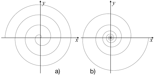
   Figure 4.9: The Archimedes’, a), and logarithmic, b), spirals.

4. The curve whose polar equation is

   $$r=a\ \mathrm{e}^{b\theta},\ \ a,b\in\mathbb{R},$$

   is the logarithmic spiral. Prove that the origin is an asymptotic point of the curve, find its curvature $c(\theta)$ and its length $\ell(\theta)$, and show that the length of the segments in which a straight line by the origin is divided by two consecutive intersections with the spiral varies as a geometrical progression. Then, prove its equiangular property: The angle $\alpha$ between $p(\theta)-o$ and $\boldsymbol{\tau}(\theta)$ is constant. Finally, show that the evolute of the logarithmic spiral is a logarithmic spiral itself (an hence that its involute is still a logarithmic spiral, that’s why Jc. Bernoulli coined for this curve the Latin sentence eadem mutata resurgo.)

5. The curve whose parametric equation is

   $$p(\theta)=a(\cos\theta+\theta\sin\theta)\mathbf{e}_{1}+a(\sin\theta-\theta\cos\theta)\mathbf{e}_{2}$$

   with $\theta$ the angle formed by $p(\theta)-o$ with the axis $x_{1}$, is the involute of the circle, Fig. 4.10. Find its curvature $c(\theta)$ and its length $\ell(\theta)$, and prove that its evolute is exactly the circle of center $o$ and radius $a$ (that is why the involute of the circle is used to profile gears).

   

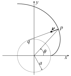
   Figure 4.10: The involute of the circle and its evolute, the circle.

6. The curve whose parametric equation is

   $$p(\theta)=a\cos\omega\theta\mathbf{e}_{1}+a\sin\omega\theta\mathbf{e}_{2}+b\omega\theta\mathbf{e}_{3}$$

   is a circular helix, i.e. a helix that winds on a circular cylinder of radius $a$, Fig. 4.11. Show that the angle $\varphi$ formed by the helix and any generatrix of the cylinder is constant (a property that defines a helix in the general case). Then, find its length $\ell(\theta)$, its curvature $c(\theta)$, torsion $\vartheta(\theta)$, and the pitch $d$, i.e., the distance between two successive intersections of the helix with a generatrix of the cylinder. Prove then the Bertrand’s theorem: A curve is a cylindrical helix if and only if the ratio $c/\vartheta=const.$ Finally, prove that for the above circular helix there are two constants $A$ and $B$ such that

   $$p^{\prime}\times p^{\prime\prime}=A\mathbf{u}(\theta)+B\mathbf{e}_{3},$$

   with

   $$\mathbf{u}=\sin\omega\theta\mathbf{e}_{1}-\cos\omega\theta\mathbf{e}_{2};$$

   then, find $A$ and $B$.

   

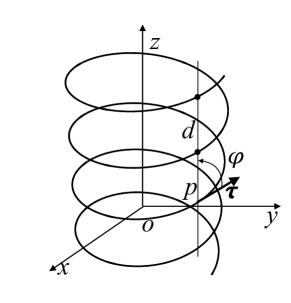
   Figure 4.11: The circular helix.

7. Find the equation of the cycloid, i.e. of the curve that is the trace of a point of a circle of radius $r$ rolling without slipping on a horizontal axis, see Fig. 4.12. Calculate the length of the cycloid for a complete round of the circle, determine its curvature, and show that the evolute of the cycloid is the cycloid itself (Huygens, 1659).

   

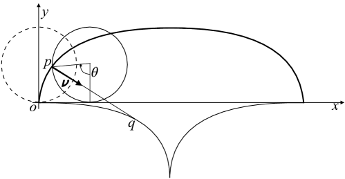
   Figure 4.12: The cycloid and its evolute.

8. The planar curve whose parametric equation is

   $$p(t)=t\mathbf{e}_{1}+\cosh t\mathbf{e}_{2}$$

   is the catenary (Jc. Bernoulli, 1690; Jn. Bernoulli, Leibniz, Huygens, 1691). It is the equilibrium curve of a heavy, perfectly flexible, and inextensible cable. Calculate the curvature of the catenary and the equation of its evolute and of its involutes (see Fig. 4.8).

9. The planar curve whose parametric equation is

   $$p(t)=\left(\cos t+\ln\tan\frac{t}{2}\right)\mathbf{e}_{1}+\sin t\mathbf{e}_{2}$$

   is the tractrix (Perrault, 1670; Newton, 1676; Huygens, 1693). This is the curve along which an object moves, under the influence of friction, when pulled on a horizontal plane by a line segment attached to a tractor that moves at a right angle to the initial line between the object and the puller at an infinitesimal speed, see Fig. 4.13. Show that the length of the tangent to the tractrix between the points on the tractrix itself and the axis $x$ is constant $\forall t$, calculate the length of the curve between $t_{1}$ and $t_{2}$, calculate the curvature of the tractrix, and finally show that its evolute is the catenary.

   

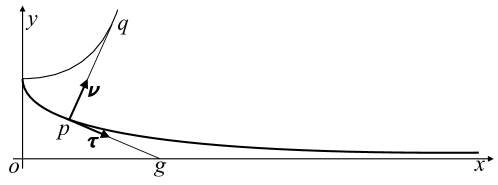
   Figure 4.13: The tractrix and its evolute.

10. For the curve whose cylindrical equation is

    $$\left\{\begin{split}&r=1,\\ &z=\sin\theta\end{split}\right.$$

    find the highest curvature and determine whether or not it is planar.

11. Let $p=p(t)$ be the path of a moving particle of masse $m$, with $t$ being the time. Define the velocity and the acceleration of $p$ as, respectively, the first and the second derivative of $p$ with respect to $t$. Decompose these two vectors in the Frenet-Serret basis and interpret physically the result. Recalling the second Newton’s principle of mechanics, what about the forces on $p$?

Chapter 5 Tensor analysis: fields

5.1 Scalar, vector and tensor fields

Let $\Omega\subset\mathcal{E}$ and $\mathbf{f}:\Omega\rightarrow\mathcal{V}$. We say that $\mathbf{f}$ is continuous at $p\in\Omega\iff\forall$ sequence $\pi_{n}=\{p_{n}\in\Omega,n\in\mathbb{N}\}$ that converges to $p\in\mathcal{E}$, the sequence $\{\mathbf{v}_{n}=\mathbf{f}(p_{n}),n\in\mathbb{N}\}$ converges to $\mathbf{f}(p)$ in $\mathcal{V}$. The function $\mathbf{f}(p):\Omega\rightarrow\mathcal{V}$ is a vector field on $\Omega$ if it is continuous at each $p\in\Omega$. In the same way we can define a scalar field $\varphi(p):\Omega\rightarrow\mathbb{R}$ and a tensor field, $\mathbf{L}(p):\Omega\rightarrow Lin(\mathcal{V})$.

A deformation is any continuous and bijective function $f(p):\Omega\rightarrow\mathcal{E}$, i.e. any transformation of a region $\Omega\subset\mathcal{E}$ into another region of $\mathcal{E}$; bijectivity imposes that to any point $p\in\Omega$ corresponds one and only one point in the transformed region, and vice-versa, which is the mathematical condition expressing the physical constraint of mass conservation.

Finally, the basic difference between fields/deformations and curves, is that a field or a deformation is defined over a subset of $\mathcal{E}$, not of $\mathbb{R}$. In practice, this implies that the components of the field/deformation are functions of three variables, the coordinates $x_{i}$ of a point $p\in\Omega$.

5.2 Differentiation of fields, differential operators

Let $\psi(p)$ be a scalar or vector or tensor field or also a deformation; we define directional derivative of $\psi(p)$ in the direction of $\mathbf{e}\in\mathcal{S}$ the limit

$$\frac{d\psi(p)}{d\mathbf{e}}:=\lim_{\alpha\rightarrow 0}\frac{\psi(p+\alpha\mathbf{e})-\psi(p)}{\alpha},\ \ \ \alpha\in\mathbb{R}.$$

The directional derivative measures the rate of variation of $\psi(p)$ in the direction of $\mathbf{e}$. In the particular case of $\mathbf{e}=\mathbf{e}_{\mathit{i}},\ i=1,2,3$, i.e. of the directions of the basis $\{\mathbf{e}_{1},\mathbf{e}_{2},\mathbf{e}_{3}\}$ of $\mathcal{V}$, then

$$\frac{d\psi(p)}{d\mathbf{e}_{\mathit{i}}}=\lim_{\alpha\rightarrow 0}\frac{\psi(p+\alpha\mathbf{e}_{\mathit{i}})-\psi(p)}{\alpha}$$

is the partial derivative of $\psi$ with respect to $x_{i}$; e.g., if $i=1$, then

$$\frac{d\psi(p)}{d\mathbf{e}_{1}}=\lim_{\alpha\rightarrow 0}\frac{\psi(x_{1}+\alpha,x_{2},x_{3})-\psi(x_{1},x_{2},x_{3})}{\alpha}.$$

The partial derivative with respect to $x_{i}$ is usually indicated as $\dfrac{\partial\psi}{\partial x_{i}}$ or also as $\psi_{,i}$.

Let $\mathbf{v}(p):\Omega\rightarrow\mathcal{V}$; we say that $\mathbf{v}$ is differentiable in $p_{0}\in\Omega\iff\exists\ \mathrm{grad}\mathbf{v}\in Lin(\mathcal{V})$ such that

$$\mathbf{v}(p_{0}+\mathbf{u})=\mathbf{v}(p)+\mathrm{grad}\mathbf{v}(p)\ \mathbf{u}+o(u)$$

when $\mathbf{u}\rightarrow\mathbf{o}$. If $\mathbf{v}$ is differentiable $\forall p\in\Omega,\mathrm{grad}\mathbf{v}$ defines a tensor field on $\Omega$ called the gradient of $\mathbf{v}$. It is also possible to define higher order differential operators, using higher order tensors, but this will not be done here. If $\mathbf{v}$ is continuous with $\mathrm{grad}\mathbf{v}\ \forall p\in\Omega$, then $\mathbf{v}$ is of class C¹ (smooth).

Let $\mathbf{v}$ be a vector field of class C¹ on $\Omega$. Then, the divergence of $\mathbf{v}$ is the scalar field defined by

$$\mathrm{div}\mathbf{v}:=\mathrm{tr}(\mathrm{grad}\mathbf{v}),$$

while $\mathrm{curl}\mathbf{v}$ is the unique vector field that satisfies the relation

$$(\mathrm{grad}\mathbf{v}-\mathrm{grad}\mathbf{v}^{\top})\mathbf{u}=(\mathrm{curl}\mathbf{v})\times\mathbf{u}\ \ \forall\mathbf{u}\in\mathcal{V}.$$

The divergence of a tensor field $\mathbf{L}$ is the unique vector field $\mathrm{div}\mathbf{L}$ that satisfies

$$(\mathrm{div}\mathbf{L})\cdot\mathbf{u}=\mathrm{div}(\mathbf{L}^{\top}\mathbf{u})\ \ \forall\mathbf{u}=const.\in\mathcal{V}.$$

Let $\varphi(p):\Omega\rightarrow\mathbb{R}$ be a scalar field over $\Omega$. Similar to the case of vector fields, we say that $\varphi$ is differentiable at $p_{0}\in\Omega\iff\exists\ \mathrm{grad}\varphi\in\mathcal{V}$ such that

$$\varphi(p+\mathbf{u})=\varphi(p)+\mathrm{grad}\varphi(p)\cdot\mathbf{u}+o(u)$$

when $\mathbf{u}\rightarrow\mathbf{o}$. If $\varphi$ is differentiable $\forall p\in\Omega,\mathrm{grad}\varphi$ defines a vector field on $\Omega$ called the gradient of $\varphi$. If $\mathrm{grad}\varphi$ is differentiable, its gradient is the tensor $\mathrm{grad}^{II}\varphi$ called second gradient or Hessian. It is immediate to show that under continuity assumption,

$$\mathrm{grad}^{II}\varphi=(\mathrm{grad}^{II}\varphi)^{\top}.$$

A level set of a scalar field $\varphi(p)$ is the set $\mathcal{S}_{L}$ such that

$$\varphi(p)=const.\ \ \forall p\in\mathcal{S}_{L}.$$

Considering hence two points $p$ and $p+\mathbf{u}$ of the same $\mathcal{S}_{L}$, then by the definition of differentiability of $\varphi(p)$ itself, we see that $\mathrm{grad}\varphi$ is a vector that is orthogonal to $\mathcal{S}_{L}$ at $p$. The curves of $\mathcal{E}$ that are tangent to $\mathrm{grad}\varphi\ \forall p\in\Omega$ are the streamlines of $\varphi$; they have the property to be orthogonal to any $\mathcal{S}_{L}$ of $\varphi\ \forall p\in\Omega$.

$\mathrm{grad}\varphi$ allows to calculate the directional derivative of $\varphi$ along any direction $\mathbf{n}\in\mathcal{S}$ as

$$\frac{d\varphi}{d\mathbf{n}}=\mathrm{grad}\varphi\cdot\mathbf{n}.$$

The highest variation of $\varphi$ is hence in the direction of $\mathrm{grad}\varphi$, and $|\mathrm{grad}\varphi|$ is the value of this variation; we remark also that $\mathrm{grad}\varphi$ is a vector directed as the increasing values of $\varphi$.

Similarly, for a vector field $\mathbf{v}$ the directional derivative along any direction $\mathbf{n}\in\mathcal{S}$ can be computed as

$$\frac{d\mathbf{v}}{d\mathbf{n}}=\mathrm{grad}\mathbf{v}\ \mathbf{n}.$$

Let $\psi$ be a scalar of vector field of class C² at least. Then, the laplacian $\Delta\psi$ of $\psi$ is defined by

$$\Delta\psi:=\mathrm{div}(\mathrm{grad}\psi).$$

By the linearity of the trace, and hence of the divergence, we see easily that the laplacian of a vector field is the vector field whose components are the laplacian of each corresponding component of the field. A field is said to be harmonic on $\Omega$ if its laplacian is null $\forall p\in\Omega$.

The definitions given above for differentiable field, gradient and class C¹ can be repeated verbatim for a deformation $f(p):\Omega\rightarrow\mathcal{E}$.

5.3 Properties of the differential operators

The differential operators, gradient, divergence, curl and laplacian, have some interesting properties, that are useful for calculations; they are introduced in this section.

Theorem 28.

(Gradient of products). Let $\varphi,\psi$ be scalar and $\mathbf{u},\mathbf{v},\mathbf{w}$ be vector fields, with all of them differentiable. Then:

$$\begin{array}[]{ll}\mathrm{i)}&\mathrm{grad}(\varphi\psi)=\varphi\ \mathrm{grad}\psi+\psi\ \mathrm{grad}\varphi,\vskip 6.0pt plus 2.0pt minus 2.0pt\\ \mathrm{ii)}&\mathrm{grad}(\varphi\mathbf{v})=\varphi\ \mathrm{grad}\mathbf{v}+\mathbf{v}\otimes\mathrm{grad}\varphi,\vskip 6.0pt plus 2.0pt minus 2.0pt\\ \mathrm{iii)}&\mathrm{grad}(\mathbf{v}\cdot\mathbf{w})=(\mathrm{grad}\mathbf{w})^{\top}\mathbf{v}+(\mathrm{grad}\mathbf{v})^{\top}\mathbf{w}.\end{array}$$ (5.1)

Proof.

The proof is based upon the definition of gradient itself:

i)                                 $(\varphi\psi)(p+\mathbf{u})=\varphi\psi+\mathrm{grad}(\varphi\psi)\cdot\mathbf{u}+o(u),$

but also

$$\begin{split}(\varphi\psi)(p+\mathbf{u})&=\varphi(p+\mathbf{u})\psi(p+\mathbf{u})=(\varphi+\mathrm{grad}\varphi\cdot\mathbf{u}+o(u))(\psi+\mathrm{grad}\psi\cdot\mathbf{u}+o(u))\\ &=\varphi\psi+\varphi\ \mathrm{grad}\psi\cdot\mathbf{u}+\psi\ \mathrm{grad}\varphi\cdot\mathbf{u}+o(u)\\ &=\varphi\psi+(\varphi\ \mathrm{grad}\psi+\psi\ \mathrm{grad}\varphi)\cdot\mathbf{u}+o(u),\end{split}$$

so by comparison

$$\mathrm{grad}(\varphi\psi)=\varphi\mathrm{grad}\psi+\psi\mathrm{grad}\varphi.$$

ii) in the same way

$$(\varphi\mathbf{v})(p+\mathbf{u})=\varphi\mathbf{v}+\mathrm{grad}(\varphi\mathbf{v})\mathbf{u}+o(u)=\varphi\mathbf{v}+\mathrm{grad}(\varphi\mathbf{v})\mathbf{u}+o(u),$$

but also

$$\begin{split}(\varphi\mathbf{v})(p+\mathbf{u})&=\varphi(p+\mathbf{u})\mathbf{v}(p+\mathbf{u})=(\varphi+\mathrm{grad}\varphi\cdot\mathbf{u}+o(u))(\mathbf{v}+\mathrm{grad}\mathbf{v}\ \mathbf{u}+o(u))\\ &=\varphi\mathbf{v}+\varphi\mathrm{grad}\mathbf{v}\ \mathbf{u}+\mathrm{grad}\varphi\cdot\mathbf{u}\ \mathbf{v}+o(u)\\ &=\varphi\mathbf{v}+(\varphi\ \mathrm{grad}\mathbf{v}+\mathbf{v}\otimes\mathrm{grad}\mathbf{v})\mathbf{u}+o(u),\end{split}$$

so comparing the two results we get

$$\mathrm{grad}(\varphi\mathbf{v})=\varphi\ \mathrm{grad}\mathbf{v}+\mathbf{v}\otimes\mathrm{grad}\mathbf{v}.$$

iii) in the same way

$$(\mathbf{v}\cdot\mathbf{w})(p+\mathbf{u})=\mathbf{v}\cdot\mathbf{w}+\mathrm{grad}(\mathbf{v}\cdot\mathbf{w})\mathbf{u}+o(u),$$

but also

$$\begin{split}(\mathbf{v}\cdot\mathbf{w})(p+\mathbf{u})&=\mathbf{v}(p+\mathbf{u})\cdot\mathbf{w}(p+\mathbf{u})=(\mathbf{v}+\mathrm{grad}\mathbf{v}\ \mathbf{u}+o(u))\cdot(\mathbf{w}+\mathrm{grad}\mathbf{w}\ \mathbf{u}+o(u))\\ &=\mathbf{v}\cdot\mathbf{w}+\mathbf{v}\cdot(\mathrm{grad}\mathbf{w}\ \mathbf{u})+(\mathrm{grad}\mathbf{v}\ \mathbf{u})\cdot\mathbf{w}+o(u)\\ &=\mathbf{v}\cdot\mathbf{w}+((\mathrm{grad}\mathbf{w})^{\top}\mathbf{v}+(\mathrm{grad}\mathbf{v})^{\top}\mathbf{w})\cdot\mathbf{u}+o(u),\end{split}$$

whence, by comparison of the two results,

$$\mathrm{grad}(\mathbf{v}\cdot\mathbf{w})=(\mathrm{grad}\mathbf{w})^{\top}\mathbf{v}+(\mathrm{grad}\mathbf{v})^{\top}\mathbf{w}.$$

∎

Another important result, relating the gradient and the curl of a vector field, is the following theorem.

Theorem 29.

If $\mathbf{v}$ is a differentiable vector field, then

$$(\mathrm{grad}\mathbf{v})\mathbf{v}=(\mathrm{curl}\mathbf{v})\times\mathbf{v}+\dfrac{1}{2}\mathrm{grad}\mathbf{v}^{2}.$$

Proof.

$$\begin{split}(\mathrm{curl}\mathbf{v})\times\mathbf{v}&=(\mathrm{grad}\mathbf{v}-(\mathrm{grad}\mathbf{v})^{\top})\mathbf{v}=(\mathrm{grad}\mathbf{v})\mathbf{v}-(\mathrm{grad}\mathbf{v})^{\top}\mathbf{v}\\ &=(\mathrm{grad}\mathbf{v})\mathbf{v}-\dfrac{1}{2}((\mathrm{grad}\mathbf{v})^{\top}\mathbf{v}+(\mathrm{grad}\mathbf{v})^{\top}\mathbf{v}),\end{split}$$

and by property iii) of the previous theorem,

$$(\mathrm{grad}\mathbf{v})^{\top}\mathbf{v}+(\mathrm{grad}\mathbf{v})^{\top}\mathbf{v}=\mathrm{grad}(\mathbf{v}\cdot\mathbf{v})=\mathrm{grad}\mathbf{v}^{2},$$

so that

$$(\mathrm{curl}\mathbf{v})\times\mathbf{v}=(\mathrm{grad}\mathbf{v})\mathbf{v}-\dfrac{1}{2}\mathrm{grad}\mathbf{v}^{2},$$

whence we obtain the thesis. ∎

The proof of the following properties of the gradient are left to the reader as an exercise:

$$\begin{array}[]{c}\mathrm{grad}(\mathbf{v}\cdot\mathbf{w})=(\mathrm{grad}\mathbf{w})\mathbf{v}+(\mathrm{grad}\mathbf{v})\mathbf{w}+\mathbf{v}\times\mathrm{curl}\mathbf{w}+\mathbf{w}\times\mathrm{curl}\mathbf{v},\vskip 6.0pt plus 2.0pt minus 2.0pt\\ \mathrm{grad}(\mathbf{u}\cdot\mathbf{v}\ \mathbf{w})=(\mathbf{u}\cdot\mathbf{v})\mathrm{grad}\mathbf{w}+(\mathbf{w}\otimes\mathbf{u})\mathrm{grad}\mathbf{v}+(\mathbf{w}\otimes\mathbf{v})\mathrm{grad}\mathbf{u},\vskip 6.0pt plus 2.0pt minus 2.0pt\\ \mathrm{grad}\mathbf{v}\cdot\mathrm{grad}\mathbf{v}^{\top}=\mathrm{div}((\mathrm{grad}\mathbf{v})\mathbf{v}-(\mathrm{div}\mathbf{v})\mathbf{v})+(\mathrm{div}\mathbf{v})^{2}.\end{array}$$ (5.2)

Theorem 30.

(Divergence of products). Let $\varphi,\mathbf{u},\mathbf{v},\mathbf{w},\mathbf{L}$ be differentiable scalar, vector or tensor fields. Then:

$$\begin{array}[]{ll}\mathrm{i)}&\mathrm{div}(\varphi\mathbf{v})=\varphi\mathrm{div}\mathbf{v}+\mathbf{v}\cdot\mathrm{grad}\varphi,\vskip 6.0pt plus 2.0pt minus 2.0pt\\ \mathrm{ii)}&\mathrm{div}(\mathbf{v}\otimes\mathbf{w})=\mathbf{v}\mathrm{div}\mathbf{w}+(\mathrm{grad}\mathbf{v})\mathbf{w},\vskip 6.0pt plus 2.0pt minus 2.0pt\\ \mathrm{iii)}&\mathrm{div}(\varphi\mathbf{L})=\varphi\mathrm{div}\mathbf{L}+\mathbf{L}\mathrm{grad}\varphi,\vskip 6.0pt plus 2.0pt minus 2.0pt\\ \mathrm{iv)}&\mathrm{div}(\mathbf{L}^{\top}\mathbf{v})=\mathbf{L}\cdot\mathrm{grad}\mathbf{v}+\mathbf{v}\cdot\mathrm{div}\mathbf{L},\vskip 6.0pt plus 2.0pt minus 2.0pt\\ \mathrm{v)}&\mathrm{div}(\mathbf{v}\times\mathbf{w})=\mathbf{w}\cdot\mathrm{curl}\mathbf{v}-\mathbf{v}\cdot\mathrm{curl}\mathbf{w}.\end{array}$$

Proof.

i) Using the definition of divergence and property ii) of Theorem 28, we get

$$\begin{split}\mathrm{div}(\varphi\mathbf{v})&=\mathrm{tr}(\mathrm{grad}(\varphi\mathbf{v}))=\mathrm{tr}(\varphi\ \mathrm{grad}\mathbf{v}+\mathbf{v}\otimes\mathrm{grad}\varphi)\\ &=\varphi\ \mathrm{tr}(\mathrm{grad}\mathbf{v})+\mathrm{tr}(\mathbf{v}\otimes\mathrm{grad}\varphi)=\varphi\ \mathrm{div}\mathbf{v}+\mathbf{v}\cdot\mathrm{grad}\varphi.\end{split}$$

ii) By the definition of divergence of a tensor, $\forall\mathbf{a}=const.\in\mathcal{V}$, and using the previous property along with property iii) of Theorem 28:

$$\begin{split}\mathrm{div}(\mathbf{v}\otimes\mathbf{w})\cdot\mathbf{a}&=\mathrm{div}((\mathbf{v}\otimes\mathbf{w})^{\top}\mathbf{a})=\mathrm{div}(\mathbf{w}\otimes\mathbf{v}\ \mathbf{a})=\mathrm{div}(\mathbf{v}\cdot\mathbf{a}\ \mathbf{w})\\ &=\mathbf{v}\cdot\mathbf{a}\ \mathrm{div}\mathbf{w}+\mathbf{w}\cdot\mathrm{grad}(\mathbf{a}\cdot\mathbf{v})\\ &=\mathrm{div}\mathbf{w}\ \mathbf{v}\cdot\mathbf{a}+\mathbf{w}\cdot(\mathrm{grad}\mathbf{v})^{\top}\mathbf{a}+\mathbf{w}\cdot(\mathrm{grad}\mathbf{a})^{\top}\mathbf{v}\\ &=(\mathbf{v}\mathrm{div}\mathbf{w}+\mathrm{grad}\mathbf{v}\ \mathbf{w})\cdot\mathbf{a}.\end{split}$$

iii) By the definition of divergence of a tensor, $\forall\mathbf{a}=const.\in\mathcal{V}$, and using the property i) along with the iii) of Theorem 28:

$$\begin{split}\mathrm{div}(\varphi\mathbf{L})\cdot\mathbf{a}&=\mathrm{div}((\varphi\mathbf{L})^{\top}\mathbf{a})=\mathrm{div}(\varphi\mathbf{L}^{\top}\mathbf{a})=\varphi\mathrm{div}(\mathbf{L}^{\top}\mathbf{a})+\mathbf{L}^{\top}\mathbf{a}\cdot\mathrm{grad}\varphi\\ &=\varphi\mathrm{div}\mathbf{L}\cdot\mathbf{a}+\mathbf{a}\cdot\mathbf{L}\mathrm{grad}\varphi=(\varphi\mathrm{div}\mathbf{L}+\mathbf{L}\mathrm{grad}\varphi)\cdot\mathbf{a}.\end{split}$$

iv) By the definition of divergence of a tensor and using the previous property:

$$\begin{split}\mathrm{div}(\mathbf{L}^{\top}\mathbf{v})&=\mathrm{div}(\mathbf{L}^{\top}v_{j}\mathbf{e}_{\mathit{j}})=\mathrm{div}((v_{j}\mathbf{L}^{\top})\mathbf{e}_{\mathit{j}})=\mathrm{div}(v_{j}\mathbf{L}^{\top})^{\top}\cdot\mathbf{e}_{\mathit{j}}\\ &=\mathrm{div}(v_{j}\mathbf{L})\cdot\mathbf{e}_{\mathit{j}}=v_{j}\mathrm{div}\mathbf{L}\cdot\mathbf{e}_{\mathit{j}}+\mathbf{L}\ \mathrm{grad}v_{j}\cdot\mathbf{e}_{\mathit{j}}\\ &=\mathbf{v}\cdot\mathrm{div}\mathbf{L}+(L_{pq}\mathbf{e}_{\mathit{p}}\otimes\mathbf{e}_{\mathit{q}}(\mathrm{grad}v_{j})_{m}\mathbf{e}_{m})\cdot\mathbf{e}_{\mathit{j}}\\ &=\mathbf{v}\cdot\mathrm{div}\mathbf{L}+L_{pq}v_{j,m}\delta_{qm}\delta_{jp}=\mathbf{v}\cdot\mathrm{div}\mathbf{L}+\mathbf{L}\cdot\mathrm{grad}\mathbf{v}.\end{split}$$

v) This property can be proved making use of the expression of the cross product with the Ricci’s alternator, given in Eq. (2.26):

$$\mathrm{curl}\mathbf{v}=\epsilon_{ijk}v_{k,j}\mathbf{e}_{\mathit{i}}$$

and

$$\mathbf{v}\times\mathbf{w}=\epsilon_{ijk}v_{j}w_{k}\mathbf{e}_{\mathit{i}},$$

whence

$$\mathrm{div}(\mathbf{v}\times\mathbf{w})=\mathrm{div}(\epsilon_{ijk}v_{j}w_{k}\mathbf{e}_{\mathit{i}})=\epsilon_{ijk}(v_{j}w_{k})_{,i}=\epsilon_{ijk}v_{j,i}w_{k}+\epsilon_{ijk}w_{k,i}v_{j}.$$

Moreover,

$$\mathbf{w}\cdot\mathrm{curl}\mathbf{v}=w_{m}\mathbf{e}_{m}\cdot\epsilon_{pqr}v_{r,q}\mathbf{e}_{\mathit{p}}=\epsilon_{pqr}v_{r,q}w_{m}\delta_{pm}=\epsilon_{pqr}v_{r,q}w_{p}=\epsilon_{qrp}v_{r,q}w_{p}$$

and

$$\mathbf{v}\cdot\mathrm{curl}\mathbf{w}=v_{m}\mathbf{e}_{m}\cdot\epsilon_{pqr}w_{r,q}\mathbf{e}_{\mathit{p}}=\epsilon_{pqr}w_{r,q}v_{m}\delta_{pm}=\epsilon_{pqr}w_{r,q}v_{p}=-\epsilon_{qpr}w_{r,q}v_{p},$$

so finally, comparing the last three results (all the subscripts are dummy indexes, so their denomination is inessential),

$$\mathrm{div}(\mathbf{v}\times\mathbf{w})=\mathbf{w}\cdot\mathrm{curl}\mathbf{v}-\mathbf{v}\cdot\mathrm{curl}\mathbf{w}.$$

∎

The divergence has also the following properties

$$\begin{array}[]{c}\mathrm{div}(\mathrm{grad}\mathbf{v}^{\top})=\mathrm{grad}(\mathrm{div}\mathbf{v}),\vskip 6.0pt plus 2.0pt minus 2.0pt\\ \mathrm{div}((\mathrm{grad}\mathbf{v})\mathbf{v})=\mathrm{grad}\mathbf{v}\cdot\mathrm{grad}\mathbf{v}^{\top}+\mathbf{v}\cdot\mathrm{grad}(\mathrm{div}\mathbf{v}),\vskip 6.0pt plus 2.0pt minus 2.0pt\\ \mathrm{div}(\varphi\mathbf{L}\mathbf{v})=\varphi\mathbf{L}^{\top}\cdot\mathrm{grad}\mathbf{v}+\varphi\mathbf{v}\cdot\mathrm{div}\mathbf{L}^{\top}+\mathbf{L}\mathbf{v}\cdot\mathrm{grad}\varphi,\end{array}$$ (5.3)

whose proof is a good exercise for the reader.

The relations of gradient and divergence with the curl are given by the following theorem.

Theorem 31.

Let $\varphi$ and $\mathbf{v}$ be scalar and vector fields of class C²; then

$$\begin{array}[]{ll}\mathrm{i)}&\mathrm{div}(\mathrm{curl}\mathbf{v})=0,\vskip 6.0pt plus 2.0pt minus 2.0pt\\ \mathrm{ii)}&\mathrm{curl}(\mathrm{grad}\varphi)=\mathbf{o}.\end{array}$$

Proof.

i) Using again the Ricci’s alternator to represent the cross product,

$$\begin{split}\mathrm{div}(\mathrm{curl}\mathbf{v})&=\mathrm{div}(\epsilon_{ijk}v_{k,j}\mathbf{e}_{\mathit{i}})=\epsilon_{ijk}v_{k,j}\mathrm{div}\mathbf{e}_{\mathit{i}}+\epsilon_{ijk}v_{k,ji}=\epsilon_{ijk}v_{k,ji}\\ &=v_{3,21}+v_{1,32}+v_{2,13}-v_{2,31}-v_{3,12}-v_{1,23}=0.\end{split}$$

ii) In a similar manner,

$$\mathrm{curl}(\mathrm{grad}\varphi)=\epsilon_{ijk}\varphi_{,kj}\mathbf{e}_{\mathit{i}}=\varphi_{32}+\varphi_{,13}+\varphi_{,21}-\varphi_{,23}-\varphi_{,31}-\varphi_{,12}=0.$$

∎

The following theorem gives an interesting relation between the curl of a vector and the divergence of its axial tensor.

Theorem 32.

(Curl of an axial vector). Let $\mathbf{w}$ be a differentiable vector field and $\mathbf{W}$ its axial tensor field. Then,

$$\mathrm{curl}\mathbf{w}=-\mathrm{div}\mathbf{W}.$$

Proof.

Using properties iv) and v) of Theorem 30 and because $\mathbf{W}=-\mathbf{W}^{\top},\forall\mathbf{a}=const.\in\mathcal{V}$ we get

$$\begin{array}[]{c}\mathrm{div}(\mathbf{w}\times\mathbf{a})=\mathbf{a}\cdot\mathrm{curl}\mathbf{w}-\mathbf{w}\cdot\mathrm{curl}\mathbf{a}=\mathbf{a}\cdot\mathrm{curl}\mathbf{w},\vskip 6.0pt plus 2.0pt minus 2.0pt\\ \mathrm{div}(\mathbf{W}\mathbf{a})=\mathrm{div}(-\mathbf{W}^{\top}\mathbf{a})=-\mathbf{W}\cdot\mathrm{grad}\mathbf{a}-\mathbf{a}\cdot\mathrm{div}\mathbf{W}=-\mathbf{a}\cdot\mathrm{div}\mathbf{W}.\end{array}$$

Now, because $\forall\mathbf{a},\mathbf{w}\times\mathbf{a}=\mathbf{W}\mathbf{a}\Rightarrow\mathrm{div}(\mathbf{w}\times\mathbf{a})=\mathrm{div}(\mathbf{W}\mathbf{a})$, we get the thesis. ∎

The way the curl of a curl is computed is given by the following theorem.

Theorem 33.

(Curl of a curl). Let $\mathbf{v}$be a vector field of class $\geq$C². Then,

$$\mathrm{curl}(\mathrm{curl}\mathbf{v})=\mathrm{grad}(\mathrm{div}\mathbf{v})-\Delta\mathbf{v}.$$

Proof.

Using properties iv) and v) of Theorem 30, along with the first of Eq. (5.3), $\forall\mathbf{a}=const.\in\mathcal{V}$ we get

$$\mathrm{div}((\mathrm{curl}\mathbf{v})\times\mathbf{a})=\mathbf{a}\cdot\mathrm{curl}(\mathrm{curl}\mathbf{v})-\mathrm{curl}\mathbf{v}\cdot\mathrm{curl}\mathbf{a}=\mathbf{a}\cdot\mathrm{curl}(\mathrm{curl}\mathbf{v}),$$

and by the definition of curl and laplacian

$$\begin{split}\mathrm{div}((\mathrm{curl}\mathbf{v})\times\mathbf{a})&=\mathrm{div}((\mathrm{grad}\mathbf{v}-(\mathrm{grad}\mathbf{v})^{\top})\mathbf{a})=\mathrm{div}(\mathrm{grad}\mathbf{v}\ \mathbf{a})-\mathrm{div}((\mathrm{grad}\mathbf{v})^{\top}\mathbf{a})\\ &=(\mathrm{grad}\mathbf{v})^{\top}\cdot\mathrm{grad}\mathbf{a}+\mathbf{a}\cdot\mathrm{div}(\mathrm{grad}\mathbf{v})^{\top}-\mathrm{grad}\mathbf{v}\cdot\mathrm{grad}\mathbf{a}-\mathbf{a}\cdot\mathrm{div}(\mathrm{grad}\mathbf{v})\\ &=\mathbf{a}\cdot(\mathrm{div}(\mathrm{grad}\mathbf{v})^{\top}-\mathrm{div}(\mathrm{grad}\mathbf{v}))=\mathbf{a}\cdot(\mathrm{grad}(\mathrm{div}\mathbf{v})-\Delta\mathbf{v}),\end{split}$$

whence, by comparison,

$$\mathrm{curl}(\mathrm{curl}\mathbf{v})=\mathrm{grad}(\mathrm{div}\mathbf{v})-\Delta\mathbf{v}.$$

∎

The proof of the following properties of the curl are can be done using the above results and it is a good exercise:

$$\begin{array}[]{c}\mathrm{curl}(\varphi\mathbf{v})=\varphi\mathrm{curl}\mathbf{v}+\mathrm{grad}\varphi\times\mathbf{v},\vskip 6.0pt plus 2.0pt minus 2.0pt\\ \mathrm{curl}(\mathbf{v}\times\mathbf{w})=(\mathrm{grad}\mathbf{v})\mathbf{w}-(\mathrm{grad}\mathbf{w})\mathbf{v}+\mathbf{v}\mathrm{div}\mathbf{w}-\mathbf{w}\mathrm{div}\mathbf{v}.\end{array}$$ (5.4)

Finally, we have a theorem also for the laplacian of a product.

Theorem 34.

(Laplacian of products). Let $\varphi,\psi,\mathbf{u},\mathbf{v}$ be scalar and vector fields of class $\geq$C². Then:

$$\begin{array}[]{ll}\mathrm{i)}&\Delta(\varphi\psi)=2\mathrm{grad}\varphi\cdot\mathrm{grad}\psi+\varphi\Delta\psi+\psi\Delta\varphi,\vskip 6.0pt plus 2.0pt minus 2.0pt\\ \mathrm{ii)}&\Delta(\mathbf{v}\cdot\mathbf{w})=2\mathrm{grad}\mathbf{v}\cdot\mathrm{grad}\mathbf{w}+\mathbf{v}\cdot\Delta\mathbf{w}+\mathbf{w}\cdot\Delta\mathbf{v}.\end{array}$$

Proof.

i) Using properties i) of Theorems 28 and 30, we get

$$\begin{split}\Delta(\varphi\psi)&=\mathrm{div}(\mathrm{grad}(\varphi\psi))=\mathrm{div}(\varphi\ \mathrm{grad}\psi+\psi\ \mathrm{grad}\varphi)\\ &=\mathrm{div}(\varphi\ \mathrm{grad}\psi)+\mathrm{div}(\psi\ \mathrm{grad}\varphi)\\ &=\varphi\ \mathrm{div}(\mathrm{grad}\psi)+\mathrm{grad}\psi\cdot\mathrm{grad}\varphi+\psi\ \mathrm{div}(\mathrm{grad}\varphi)+\mathrm{grad}\varphi\cdot\mathrm{grad}\psi\\ &=2\mathrm{grad}\varphi\cdot\mathrm{grad}\psi+\varphi\ \Delta\psi+\psi\ \Delta\varphi.\end{split}$$

ii) Using properties iii) of Theorem 28 and iv) of Theorem 30, we obtain

$$\begin{split}\Delta(\mathbf{v}\cdot\mathbf{w})&=\mathrm{div}(\mathrm{grad}(\mathbf{v}\cdot\mathbf{w}))=\mathrm{div}((\mathrm{grad}\mathbf{w})^{\top}\mathbf{v}+(\mathrm{grad}\mathbf{v})^{\top}\mathbf{w})\\ &=\mathrm{div}((\mathrm{grad}\mathbf{w})^{\top}\mathbf{v})+\mathrm{div}((\mathrm{grad}\mathbf{v})^{\top}\mathbf{w})\\ &=\mathrm{grad}\mathbf{w}\cdot\mathrm{grad}\mathbf{v}+\mathbf{v}\cdot\mathrm{div}(\mathrm{grad}\mathbf{w})+\mathrm{grad}\mathbf{v}\cdot\mathrm{grad}\mathbf{w}+\mathbf{w}\cdot\mathrm{div}(\mathrm{grad}\mathbf{v})\\ &=2\mathrm{grad}\mathbf{v}\cdot\mathrm{grad}\mathbf{w}+\mathbf{v}\cdot\Delta\mathbf{w}+\mathbf{w}\cdot\Delta\mathbf{v}.\end{split}$$

∎

5.4 Theorems on fields

We recall here some classical theorems on fields and operators.

Theorem 35.

(Harmonic fields). If $\mathbf{v}(p)$ is a vector field of class $\geq\mathrm{C}^{2}$ such that

$$\mathrm{div}\mathbf{v}=0,\ \ \ \mathrm{curl}\mathbf{v}=\mathbf{o},$$

then $\mathbf{v}$ is harmonic: $\Delta\mathbf{v}=\mathbf{o}$.

Proof.

By the definition of curl,

$$\mathrm{curl}\mathbf{v}=\mathbf{o}\Rightarrow\ \mathrm{grad}\mathbf{v}-(\mathrm{grad}\mathbf{v})^{\top}=\mathbf{o}\Rightarrow\mathrm{div}(\mathrm{grad}\mathbf{v}-(\mathrm{grad}\mathbf{v})^{\top})=\mathbf{o},$$

and through Eq. (5.3)₁, the definition of laplacian and because by hypothesis $\mathrm{div}\mathbf{v}=0$, we have

$$\mathrm{div}(\mathrm{grad}\mathbf{v}-(\mathrm{grad}\mathbf{v})^{\top})=\Delta\mathbf{v}-\mathrm{grad}(\mathrm{div}\mathbf{v})=\Delta\mathbf{v}.$$

∎

We state now without proof a lemma that, basically, allows us to transform a volume integral on a domain $\Omega$ to a surface integral on the boundary surface $\partial\Omega$.

Theorem 36.

(Divergence lemma). Let $\mathbf{v}(p)$ be a vector field of class $\geq\mathrm{C}^{1}$ on a regular region $\Omega\subset\mathcal{E}$. Then,

$$\int_{\partial\Omega}\mathbf{v}\otimes\mathbf{n}\ dA=\int_{\Omega}\mathrm{grad}\mathbf{v}\ dV.$$

This lemma is fundamental for proving the three forms of the Gauss theorem, which is of the paramount importance in many fields of mathematical physics.

Theorem 37.

(Divergence or Gauss theorem). Let $\varphi,\mathbf{v},\mathbf{L}$ be, respectively, a scalar, vector and tensor field of class $\geq\mathrm{C}^{1}$ on a regular region $\Omega\subset\mathcal{E}$ . Then:

$$\begin{split}&\mathrm{i)}\ \ \int_{\partial\Omega}\varphi\mathbf{n}\ dA=\int_{\Omega}\mathrm{grad}\varphi\ dV,\vskip 6.0pt plus 2.0pt minus 2.0pt\\ &\mathrm{ii)}\ \int_{\partial\Omega}\mathbf{v}\cdot\mathbf{n}\ dA=\int_{\Omega}\mathrm{div}\mathbf{v}\ dV,\vskip 6.0pt plus 2.0pt minus 2.0pt\\ &\mathrm{iii)}\int_{\partial\Omega}\mathbf{L}\mathbf{n}\ dA=\int_{\Omega}\mathrm{div}\mathbf{L}\ dV.\end{split}$$

Proof.

i) $\forall\mathbf{a}=const.\in\mathcal{V}$, by the lemma of divergence,

$$\int_{\Omega}\mathrm{grad}(\varphi\mathbf{a})dV=\int_{\partial\Omega}\varphi\mathbf{a}\otimes\mathbf{n}\ dA=\mathbf{a}\otimes\int_{\partial\Omega}\varphi\mathbf{n}\ dA,$$

but also, by ii) of Theorem 28,

$$\int_{\Omega}\mathrm{grad}(\varphi\mathbf{a})dV=\int_{\Omega}(\varphi\ \mathrm{grad}\mathbf{a}+\mathbf{a}\otimes\mathrm{grad}\varphi)dV=\mathbf{a}\otimes\int_{\Omega}\mathrm{grad}\varphi\ dV,$$

whence, by comparison,

$$\int_{\partial\Omega}\varphi\mathbf{n}\ dA=\int_{\Omega}\mathrm{grad}\varphi\ dV.$$

ii) Again by the divergence lemma,

$$\mathrm{tr}\int_{\Omega}\mathrm{grad}\mathbf{v}\ dV=\mathrm{tr}\int_{\partial\Omega}\mathbf{v}\otimes\mathbf{n}\ dA=\int_{\partial\Omega}\mathrm{tr}(\mathbf{v}\otimes\mathbf{n})dA=\int_{\partial\Omega}\mathbf{v}\cdot\mathbf{n}\ dA,$$

but also

$$\mathrm{tr}\int_{\Omega}\mathrm{grad}\mathbf{v}\ dV=\int_{\Omega}\mathrm{tr}(\mathrm{grad}\mathbf{v})dV=\int_{\Omega}\mathrm{div}\mathbf{v}\ dV,$$

so, by comparison,

$$\int_{\partial\Omega}\mathbf{v}\cdot\mathbf{n}\ dA=\int_{\Omega}\mathrm{div}\mathbf{v}\ dV.$$

iii) $\forall\mathbf{a}=const.\in\mathcal{V}$, by the lemma of divergence, property iv) of Theorem 30 and ii) just proved,

$$\int_{\Omega}\mathrm{div}(\mathbf{L}^{\top}\mathbf{a})dV=\int_{\partial\Omega}(\mathbf{L}^{\top}\mathbf{a})\cdot\mathbf{n}\ dA=\int_{\partial\Omega}\mathbf{a}\cdot\mathbf{L}\mathbf{n}\ dA=\mathbf{a}\cdot\int_{\partial\Omega}\mathbf{L}\mathbf{n}\ dA,$$

but also

$$\int_{\Omega}\mathrm{div}(\mathbf{L}^{\top}\mathbf{a})dV=\int_{\Omega}(\mathrm{div}\mathbf{L})\cdot\mathbf{a}+\mathbf{L}\cdot\mathrm{grad}\mathbf{a}\ dV=\mathbf{a}\cdot\int_{\Omega}\mathrm{div}\mathbf{L}\ dV,$$

so, once more by comparison,

$$\int_{\partial\Omega}\mathbf{L}\mathbf{n}\ dA=\int_{\Omega}\mathrm{div}\mathbf{L}\ dV.$$

∎

The following identities follow directly from the Gauss theorem:

$$\begin{split}&\int_{\partial\Omega}\mathbf{v}\cdot\mathbf{L}\mathbf{n}\ dA=\int_{\Omega}(\mathbf{v}\cdot\mathrm{div}\mathbf{L}+\mathbf{L}\cdot\mathrm{grad}\mathbf{v})dV,\\ &\int_{\partial\Omega}(\mathbf{L}\mathbf{n})\otimes\mathbf{v}\ dA=\int_{\Omega}((\mathrm{div}\mathbf{L})\otimes\mathbf{v}+\mathbf{L}(\mathrm{grad}\mathbf{v}^{\top}))dV,\\ &\int_{\partial\Omega}(\mathbf{w}\cdot\mathbf{n})\mathbf{v}\ dA=\int_{\Omega}(\mathbf{v}\mathrm{div}\mathbf{w}+(\mathrm{grad}\mathbf{v})\mathbf{w})dV.\end{split}$$ (5.5)

A direct consequence of the Gauss theorem is the following result.

Theorem 38.

(Flux theorem). Let $\mathbf{v}(p)$ be a vector field of class $\geq\mathrm{C}^{1}$ on an open subset $\mathtt{R}$ of $\mathcal{E}$. Then,

$$\mathrm{div}\mathbf{v}=0\iff\int_{\partial\Omega}\mathbf{v}\cdot\mathbf{n}\ dA=0\ \ \ \forall\Omega\subset\mathtt{R}.$$

Proof.

It immediately follows from the ii) of the Gauss theorem. ∎

Another consequence of the Gauss Theorem is the next theorem.

Theorem 39.

(Curl theorem). Let $\mathbf{v}(p)$ be a vector field of class $\geq\mathrm{C}^{1}$ on a regular region $\Omega\subset\mathcal{E}$; then

$$\int_{\partial\Omega}\mathbf{n}\times\mathbf{v}\ dA=\int_{\Omega}\mathrm{curl}\mathbf{v}\ dV.$$

Proof.

If $\mathbf{V}$ is the axial tensor of $\mathbf{v}$, by Theorem 32 and iii) of the Gauss theorem,

$$\int_{\partial\Omega}\mathbf{n}\times\mathbf{v}\ dA=-\int_{\partial\Omega}\mathbf{v}\times\mathbf{n}\ dA=-\int_{\partial\Omega}\mathbf{V}\mathbf{n}\ dA=-\int_{\Omega}\mathrm{div}\mathbf{V}\ dV=\int_{\Omega}\mathrm{curl}\mathbf{v}\ dV.$$

∎

The following classical theorems on fields are recalled here without proof.

Theorem 40.

(Potential theorem). Let $\mathbf{v}(p)$ be a vector field of class $\geq\mathrm{C}^{1}$ on a simply connected region $\Omega\subset\mathcal{E}$. Then,

$$\mathrm{curl}\mathbf{v}=\mathbf{o}\iff\mathbf{v}=\mathrm{grad}\varphi$$

with $\varphi(p)$ the potential, a scalar field of class $\geq\mathrm{C}^{2}$.

Theorem 41.

(Stokes theorem). Let $\mathbf{v}(p)$ be a vector field of class $\geq\mathrm{C}^{1}$ on a regular region $\Omega\subset\mathcal{E}$, $\Sigma$ an open surface whose support is the closed line $\gamma$ and $\mathbf{n}\in\mathcal{S}$ the normal to $\Sigma$, see Fig. 5.1. Then,

$$\oint_{\gamma}\mathbf{v}\cdot d\ell=\int_{\Sigma}\mathrm{curl}\mathbf{v}\cdot\mathbf{n}\ dA.$$

The parametric equation of $\gamma$ must be chosen in such a way that

$$p^{\prime}(t_{1})\times p^{\prime}(t_{2})\cdot\mathbf{n}>0\ \ \ \forall t_{2}>t_{1}.$$

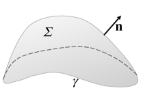
Figure 5.1: Scheme for the Stokes theorem.

Theorem 42.

(Green’s formula). Let $\varphi(p),\psi(p)$ be two scalar fields of class $\geq\mathrm{C}^{2}$ on a regular region $\Omega\subset\mathcal{E}$, with $\mathbf{n}\in\mathcal{S}$ the normal to $\partial\Omega$. Then,

$$\int_{\partial\Omega}\left(\psi\frac{d\varphi}{d\mathbf{n}}-\varphi\frac{d\psi}{d\mathbf{n}}\right)dA=\int_{\Omega}(\psi\ \Delta\varphi-\varphi\ \Delta\psi)dV.$$

5.5 Differential operators in Cartesian coordinates

The Cartesian expression of the differential operators can be found without difficulty by applying the properties of such operators shown previously and considering that the vectors of a Cartesian basis are fixed. The final result is,

$$\begin{split}&\mathrm{grad}f=f_{,i}\ \mathbf{e}_{\mathit{i}},\\ &\mathrm{grad}\mathbf{v}=v_{i,j}\mathbf{e}_{\mathit{i}}\otimes\mathbf{e}_{\mathit{j}},\\ &\mathrm{div}\mathbf{v}=v_{i,i},\\ &\mathrm{div}\mathbf{L}=L_{ij,j}\mathbf{e}_{\mathit{i}},\\ &\Delta f=f_{,ii},\\ &\Delta\mathbf{v}=\Delta v_{i}\mathbf{e}_{\mathit{i}}=v_{i,jj}\mathbf{e}_{\mathit{i}},\\ &\mathrm{curl}\mathbf{v}=(v_{3,2}-v_{2,3})\mathbf{e}_{1}+(v_{1,3}-v_{3,1})\mathbf{e}_{2}+(v_{2,1}-v_{1,2})\mathbf{e}_{3}.\end{split}$$ (5.6)

The so-called operator nabla $\nabla$,

$$\nabla:=\frac{\partial\cdot}{\partial x_{i}}\mathbf{e}_{i}=\frac{\partial\cdot}{\partial x_{1}}\mathbf{e}_{1}+\frac{\partial\cdot}{\partial x_{2}}\mathbf{e}_{2}+\frac{\partial\cdot}{\partial x_{3}}\mathbf{e}_{3}$$ (5.7)

is often used to indicate the differential operators:

$$\begin{split}&\mathrm{grad}f=\nabla f,\\ &\mathrm{div}\mathbf{v}=\nabla\cdot\mathbf{v},\\ &\mathrm{curl}\mathbf{v}=\nabla\times\mathbf{v},\\ &\Delta f=\nabla^{2}f.\end{split}$$

5.6 Differential operators in cylindrical coordinates

The cylindrical coordinates $\rho,\theta,z$ of a point $p$, whose Cartesian coordinates in the (fixed) frame $\{o;\mathbf{e}_{1},\mathbf{e}_{2},\mathbf{e}_{3}\}$ are $p=(x_{1},x_{2},x_{3})$, are shown in Fig. 5.2. They are related together by

$$\begin{split}&\rho=\sqrt{x_{1}^{2}+x_{2}^{2}},\\ &\theta=\arctan\dfrac{x_{2}}{x_{1}},\\ &z=x_{3},\end{split}$$ (5.8)

or conversely

$$\begin{split}&x_{1}=\rho\cos\theta,\\ &x_{2}=\rho\sin\theta,\\ &x_{3}=z.\end{split}$$ (5.9)

To notice that $\rho\geq 0$ and that the anomaly $\theta$ is bounded by $0\leq\theta<2\pi$.

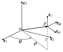
Figure 5.2: Cylindrical coordinates.

A vector $p-o=x_{i}\mathbf{e}_{\mathit{i}}$, in the cylindrical basis is expressed has

$$p-o=\rho\mathbf{e}_{\rho}+z\mathbf{e}_{\mathit{z}}$$

and the rotation tensor transforming the Cartesian basis $\{\mathbf{e}_{1},\mathbf{e}_{2},\mathbf{e}_{3}\}$ into the cylindrical one, $\{\mathbf{e}_{\rho},\mathbf{e}_{\theta},\mathbf{e}_{\mathit{z}}\}$ is

$$\mathbf{Q}=\left[\begin{array}[]{ccc}\cos\theta&-\sin\theta&0\\ \sin\theta&\cos\theta&0\\ 0&0&1\end{array}\right],$$

so the relations between the vectors of the Cartesian and the cylindrical bases are

$$\begin{split}&\mathbf{e}_{\rho}=\cos\theta\mathbf{e}_{1}+\sin\theta\mathbf{e}_{2},\\ &\mathbf{e}_{\theta}=-\sin\theta\mathbf{e}_{1}+\cos\theta\mathbf{e}_{2},\\ &\mathbf{e}_{\mathit{z}}=\mathbf{e}_{3},\end{split}$$

and viceversa

$$\begin{split}&\mathbf{e}_{1}=\cos\theta\mathbf{e}_{\rho}-\sin\theta\mathbf{e}_{\theta},\\ &\mathbf{e}_{2}=\sin\theta\mathbf{e}_{\rho}+\cos\theta\mathbf{e}_{\theta},\\ &\mathbf{e}_{3}=\mathbf{e}_{\mathit{z}}.\end{split}$$ (5.10)

The question is: How can we express the differential operators in the (moving) frame $\{p;\mathbf{e}_{\rho},\mathbf{e}_{\theta},\mathbf{e}_{z}\}$? To this end, we can proceed as follows: From Eq. (5.8)

$$f_{,i}=f_{,\rho}\frac{\partial\rho}{\partial x_{i}}+f_{,\theta}\frac{\partial\theta}{\partial x_{i}}+f_{,z}\frac{\partial z}{\partial x_{i}}\rightarrow\ \left\{\begin{split}&f_{,1}=f_{,\rho}\frac{x_{1}}{\rho}-f_{,\theta}\frac{x_{2}}{\rho^{2}},\\ &f_{,2}=f_{,\rho}\frac{x_{2}}{\rho}+f_{,\theta}\frac{x_{1}}{\rho^{2}},\\ &f_{,3}=f_{,z}.\end{split}\right.$$ (5.11)

So, by Eqs. (5.6)₁ and (5.10),

$$\mathrm{grad}f=f_{i}\mathbf{e}_{\mathit{i}}=\left(f_{,\rho}\frac{x_{1}}{\rho}-f_{,\theta}\frac{x_{2}}{\rho^{2}}\right)(\cos\theta\mathbf{e}_{\rho}-\sin\theta\mathbf{e}_{\theta})+\left(f_{,\rho}\frac{x_{2}}{\rho}+f_{,\theta}\frac{x_{1}}{\rho^{2}}\right)(\sin\theta\mathbf{e}_{\rho}+\cos\theta\mathbf{e}_{\theta})+f_{,z}\mathbf{e}_{\mathit{z}}.$$

Finally, by Eq. (5.9) and through some standard operations, we obtain

$$\mathrm{grad}f=f_{,\rho}\mathbf{e}_{\rho}+\frac{1}{\rho}f_{,\theta}\ \mathbf{e}_{\theta}+f_{,z}\mathbf{e}_{\mathit{z}}.$$

The gradient of a vector field $\mathbf{v}$ can be obtained in a similar way. If we denote by $\mathbf{v}_{Cart}$ the vector $\mathbf{v}$ expressed by its Cartesian components $(v_{1},v_{2},v_{3})$ and by $\mathbf{v}_{cyl}$ the same vector expressed through the cylindrical ones, $\{v_{\rho},v_{\theta},v_{z}\}$, then, cf. Section 2.11,

$$\mathbf{v}_{Cart}=\mathbf{Q}\mathbf{v}_{cyl}\rightarrow\left\{\begin{split}&v_{1}=v_{\rho}\cos\theta-v_{\theta}\sin\theta,\\ &v_{2}=v_{\rho}\sin\theta+v_{\theta}\cos\theta,\\ &v_{3}=v_{z}.\end{split}\right.$$ (5.12)

Applying Eq. (5.11) to these components, we get

$$\begin{split}&v_{i,1}=v_{i,\rho}\frac{x_{1}}{\rho}-v_{i,\theta}\frac{x_{2}}{\rho^{2}},\\ &v_{i,2}=v_{i,\rho}\frac{x_{2}}{\rho}+v_{i,\theta}\frac{x_{1}}{\rho^{2}},\\ &v_{i,3}=v_{i,z}.\end{split}$$ (5.13)

Injecting these expressions into Eq. (5.6)₂ for the $v_{i,j}$s and the (5.10) for the $\mathbf{e}_{\mathit{i}}$s, gives finally

$$\begin{split}\mathrm{grad}\mathbf{v}&=v_{\rho,\rho}(\mathbf{e}_{\rho}\otimes\mathbf{e}_{\rho})+\dfrac{1}{\rho}(v_{\rho,\theta}-v_{\theta})(\mathbf{e}_{\rho}\otimes\mathbf{e}_{\theta})+v_{\rho,z}(\mathbf{e}_{\rho}\otimes\mathbf{e}_{\mathit{z}})\\ &+v_{\theta,\rho}(\mathbf{e}_{\theta}\otimes\mathbf{e}_{\rho})+\dfrac{1}{\rho}(v_{\theta,\theta}+v_{\rho})(\mathbf{e}_{\theta}\otimes\mathbf{e}_{\theta})+v_{\theta,z}(\mathbf{e}_{\theta}\otimes\mathbf{e}_{\mathit{z}})\\ &+v_{z,\rho}(\mathbf{e}_{\mathit{z}}\otimes\mathbf{e}_{\rho})+\dfrac{1}{\rho}v_{z,\theta}(\mathbf{e}_{\mathit{z}}\otimes\mathbf{e}_{\theta})+v_{z,z}(\mathbf{e}_{\mathit{z}}\otimes\mathbf{e}_{\mathit{z}}),\end{split}$$

or, in matrix form,

$$\mathrm{grad}\mathbf{v}=\left[\begin{array}[]{ccc}v_{\rho,\rho}&\dfrac{1}{\rho}(v_{\rho,\theta}-v_{\theta})&v_{\rho,z}\vskip 3.0pt plus 1.0pt minus 1.0pt\\ v_{\theta,\rho}&\dfrac{1}{\rho}(v_{\theta,\theta}+v_{\rho})&v_{\theta,z}\vskip 3.0pt plus 1.0pt minus 1.0pt\\ v_{z,\rho}&\dfrac{1}{\rho}v_{z,\theta}&v_{z,z}\end{array}\right],$$

By the definition of divergence, we get immediately

$$\mathrm{div}\mathbf{v}=v_{\rho,\rho}+\dfrac{1}{\rho}(v_{\theta,\theta}+v_{\rho})+v_{z,z}.$$ (5.14)

Now, from Eq. (5.6), we see that $\mathrm{div}\mathbf{L}$ is the vector whose components are the divergence of the rows of the matrix representing $\mathbf{L}$. So, we need first to calculate the Cartesian components of $\mathbf{L}$ as functions of the cylindrical ones, cf. Section 2.11:

$$\mathbf{L}_{Cart}=\mathbf{Q}\mathbf{L}_{cyl}\mathbf{Q}^{\top}\rightarrow\left\{\begin{array}[]{l}L_{11}=-\sin\theta(L_{\rho\theta}\cos\theta-L_{\theta\theta}\sin\theta)+\cos\theta(L_{\rho\rho}\cos\theta-L_{\theta\rho}\sin\theta),\vskip 6.0pt plus 2.0pt minus 2.0pt\\ L_{12}=\cos\theta(L_{\rho\theta}\cos\theta-L_{\theta\theta}\sin\theta)+\sin\theta(L_{\rho\rho}\cos\theta-L_{\theta\rho}\sin\theta),\vskip 6.0pt plus 2.0pt minus 2.0pt\\ L_{13}=L_{\rho z}\cos\theta-L_{\theta z}\sin\theta,\vskip 6.0pt plus 2.0pt minus 2.0pt\\ L_{21}=-\sin\theta(L_{\theta\theta}\cos\theta+L_{\rho\theta}\sin\theta)+\cos\theta(L_{\theta\rho}\cos\theta+L_{\rho\rho}\sin\theta),\vskip 6.0pt plus 2.0pt minus 2.0pt\\ L_{22}=\cos\theta(L_{\theta\theta}\cos\theta+L_{\rho\theta}\sin\theta)+\sin\theta(L_{\theta\rho}\cos\theta+L_{\rho\rho}\sin\theta),\vskip 6.0pt plus 2.0pt minus 2.0pt\\ L_{23}=L_{\theta z}\cos\theta+L_{\rho z}\sin\theta,\vskip 6.0pt plus 2.0pt minus 2.0pt\\ L_{31}=L_{z\rho}\cos\theta-L_{z\theta}\sin\theta,\vskip 6.0pt plus 2.0pt minus 2.0pt\\ L_{32}=L_{z\theta}\cos\theta+L_{z\rho}\sin\theta,\vskip 6.0pt plus 2.0pt minus 2.0pt\\ L_{33}=L_{zz}.\end{array}\right.$$

Then, applying Eqs. (5.10) and (5.14) in Eq. (5.6)₃ for the vectors $\mathbf{v}_{i}=(L_{i1},L_{i2},L_{i3}),\ i=1,2,3$, we get, through long but standard passages and after putting $\theta=0$ in order to obtain the components of $\mathrm{div}\mathbf{L}$ in the basis $\{\mathbf{e}_{\rho},\mathbf{e}_{\theta},\mathbf{e}_{\mathit{z}}\}$,

$$\begin{split}\mathrm{div}\mathbf{L}&=\left(\dfrac{1}{\rho}((\rho L_{\rho\rho})_{,\rho}+L_{\rho\theta,\theta}-L_{\theta\theta})+L_{\rho z,z}\right)\mathbf{e}_{\rho}\\ &+\left(L_{\theta\rho,\rho}+\dfrac{1}{\rho}(L_{\theta\theta,\theta}+L_{\rho\theta}+L_{\theta\rho})+L_{\theta z,z}\right)\mathbf{e}_{\theta}\\ &+\left(\dfrac{1}{\rho}((\rho L_{z\rho})_{,\rho}+L_{z\theta,\theta})+L_{zz,z}\right)\mathbf{e}_{\mathit{z}}.\end{split}$$

To obtain $\Delta f=f,_{ii}$, we need to apply twice Eq. (5.11), which gives

$$\begin{split}f_{,11}&=\left(f_{,\rho}\frac{x_{1}}{\rho}-f_{,\theta}\frac{x_{2}}{\rho^{2}}\right)_{,1}=f_{,\rho 1}\frac{x_{1}}{\rho}+f_{,\rho}\frac{\rho-x_{1}\rho_{,1}}{\rho^{2}}-f_{,\theta 1}\frac{x_{2}}{\rho^{2}}+f_{,\theta}\frac{2x_{2}\rho\rho_{,1}}{\rho^{4}}\\ &=\left(f_{,\rho\rho}\frac{x_{1}}{\rho}-f_{,\rho\theta}\frac{x_{2}}{\rho^{2}}\right)\frac{x_{1}}{\rho}+f_{,\rho}\frac{\rho^{2}-x_{1}^{2}}{\rho^{3}}-\left(f_{,\rho\theta}\frac{x_{1}}{\rho}-f_{,\theta\theta}\frac{x_{2}}{\rho^{2}}\right)\frac{x_{2}}{\rho^{2}}+f_{,\theta}\frac{2x_{1}x_{2}}{\rho^{4}}\\ &=f_{,\rho\rho}\cos^{2}\theta-2f_{,\rho\theta}\frac{\sin\theta\cos\theta}{\rho}+f_{,\rho}\frac{\sin^{2}\theta}{\rho}+f_{,\theta\theta}\frac{\sin^{2}\theta}{\rho^{2}}+2f_{,\theta}\frac{\sin\theta\cos\theta}{\rho^{2}},\end{split}$$

$$\begin{split}f_{,22}&=\left(f_{,\rho}\frac{x_{2}}{\rho}+f_{,\theta}\frac{x_{1}}{\rho^{2}}\right)_{,2}=f_{,\rho 2}\frac{x_{2}}{\rho}+f_{,\rho}\frac{\rho-x_{2}\rho_{,2}}{\rho^{2}}+f_{,\theta 2}\frac{x_{1}}{\rho^{2}}-f_{,\theta}\frac{2x_{1}\rho\rho_{,2}}{\rho^{4}}\\ &=\left(f_{,\rho\rho}\frac{x_{2}}{\rho}+f_{,\rho\theta}\frac{x_{1}}{\rho^{2}}\right)\frac{x_{2}}{\rho}+f_{,\rho}\frac{\rho^{2}-x_{2}^{2}}{\rho^{3}}+\left(f_{,\rho\theta}\frac{x_{2}}{\rho}+f_{,\theta\theta}\frac{x_{1}}{\rho^{2}}\right)\frac{x_{1}}{\rho^{2}}-f_{,\theta}\frac{2x_{1}x_{2}}{\rho^{4}}\\ &=f_{,\rho\rho}\sin^{2}\theta+2f_{,\rho\theta}\frac{\sin\theta\cos\theta}{\rho}+f_{,\rho}\frac{\cos^{2}\theta}{\rho}+f_{,\theta\theta}\frac{\cos^{2}\theta}{\rho^{2}}-2f_{,\theta}\frac{\sin\theta\cos\theta}{\rho^{2}},\end{split}$$

$$f_{,33}=f_{,zz}.$$

Then, adding these terms together, we finally have

$$\Delta f=\frac{1}{\rho}(\rho f_{,\rho})_{,\rho}+\frac{1}{\rho^{2}}f_{,\theta\theta}+f_{,zz}.$$

The laplacian $\Delta\mathbf{v}$ of a vector field $\mathbf{v}$, Eq. (5.6)₆, can be obtained by following the same steps for each one of the components in Eq. (5.12), which gives

$$\begin{split}\Delta\mathbf{v}&=\left(\dfrac{1}{\rho}(\rho v_{\rho,\rho})_{,\rho}+\dfrac{1}{\rho^{2}}v_{\rho,\theta\theta}+v_{\rho,zz}-\dfrac{1}{\rho^{2}}(v_{\rho}+2v_{\theta,\theta})\right)\mathbf{e}_{\rho}\\ &+\left(\dfrac{1}{\rho}(\rho v_{\theta,\rho})_{,\rho}+\dfrac{1}{\rho^{2}}v_{\theta,\theta\theta}+v_{\theta,zz}-\dfrac{1}{\rho^{2}}(v_{\theta}-2v_{\rho,\theta})\right)\mathbf{e}_{\theta}\\ &+\left(\dfrac{1}{\rho}(\rho v_{z,\rho})_{,\rho}+\dfrac{1}{\rho^{2}}v_{z,\theta\theta}+v_{z,zz}\right)\mathbf{e}_{\mathit{z}}.\end{split}$$

Finally, injecting Eqs. (5.10), (5.12) and (5.13) into Eq. (5.6)₇ gives

$$\mathrm{curl}\mathbf{v}=\left(\dfrac{1}{\rho}v_{z,\theta}-v_{\theta,z}\right)\mathbf{e}_{\rho}+(v_{\rho,z}-v_{z,\rho})\mathbf{e}_{\theta}+\left(\dfrac{1}{\rho}((\rho v_{\theta})_{,\rho}-v_{\rho,\theta})\right)\mathbf{e}_{\mathit{z}}.$$ (5.15)

5.7 Differential operators in spherical coordinates

The spherical coordinates $r,\varphi,\theta$ of a point $p$, whose Cartesian coordinates in the (fixed) frame $\{o;\mathbf{e}_{1},\mathbf{e}_{2},\mathbf{e}_{3}\}$ are $p=(x_{1},x_{2},x_{3})$, are shown in Fig. 5.3. They are related together by

$$\begin{split}&r=\sqrt{x_{1}^{2}+x_{2}^{2}+x_{3}^{2}},\\ &\varphi=\arctan\dfrac{\sqrt{x_{1}^{2}+x_{2}^{2}}}{x_{3}},\\ &\theta=\arctan\dfrac{x_{2}}{x_{1}},\end{split}$$

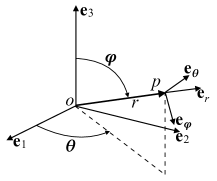
Figure 5.3: Spherical coordinates.

or conversely

$$\begin{split}&x_{1}=r\cos\theta\sin\varphi,\\ &x_{2}=r\sin\theta\sin\varphi,\\ &x_{3}=r\cos\varphi.\end{split}$$

We note that $r\geq 0$ and that the anomaly $\theta$ is bounded by $0\leq\theta<2\pi$ while the colatitude $\varphi$ by $0\leq\varphi\leq\pi$.

The procedure to determine the expression of the differential operators in spherical coordinates, i.e. in the (moving) frame $\{p;\mathbf{e}_{r},\mathbf{e}_{\varphi},\mathbf{e}_{\theta}\}$, is identical to that used for the cylindrical coordinates, but the analytical developments are even more complicated and long, so they are omitted here and only the final formulae are given in the following:

$$\mathrm{grad}f=f_{,r}\mathbf{e}_{r}+\dfrac{1}{r}f_{,\varphi}\mathbf{e}_{\varphi}+\dfrac{1}{r\sin\varphi}f_{,\theta}\mathbf{e}_{\theta},$$

$$\begin{split}\mathrm{grad}\mathbf{v}&=v_{r,r}\mathbf{e}_{r}\otimes\mathbf{e}_{r}+\dfrac{1}{r}(v_{r,\varphi}-v_{\varphi})\mathbf{e}_{r}\otimes\mathbf{e}_{\varphi}+\dfrac{1}{r}\left(\dfrac{1}{\sin\varphi}v_{r,\theta}-v_{\theta}\right)\mathbf{e}_{r}\otimes\mathbf{e}_{\theta}\\ &+v_{\varphi,r}\mathbf{e}_{\varphi}\otimes\mathbf{e}_{r}+\dfrac{1}{r}(v_{\varphi,\varphi}+v_{r})\mathbf{e}_{\varphi}\otimes\mathbf{e}_{\varphi}+\dfrac{1}{r}\left(\dfrac{1}{\sin\varphi}v_{\varphi,\theta}-v_{\theta}\cot\varphi\right)\mathbf{e}_{\varphi}\otimes\mathbf{e}_{\theta}\\ &+v_{\theta,r}\mathbf{e}_{\theta}\otimes\mathbf{e}_{r}+\dfrac{1}{r}v_{\theta,\varphi}\mathbf{e}_{\theta}\otimes\mathbf{e}_{\varphi}+\dfrac{1}{r}\left(\dfrac{1}{\sin\varphi}v_{\theta,\theta}+v_{r}+v_{\varphi}\cot\varphi\right)\mathbf{e}_{\theta}\otimes\mathbf{e}_{\theta},\end{split}$$

or, in matrix form,

$$\mathrm{grad}\mathbf{v}=\left[\begin{array}[]{ccc}v_{r,r}&\dfrac{1}{r}(v_{r,\varphi}-v_{\varphi})&\dfrac{1}{r}\left(\dfrac{1}{\sin\varphi}v_{r,\theta}-v_{\theta}\right)\\ v_{\varphi,r}&\dfrac{1}{r}(v_{\varphi,\varphi}+v_{r})&\dfrac{1}{r}\left(\dfrac{1}{\sin\varphi}v_{\varphi,\theta}-v_{\theta}\cot\varphi\right)\\ v_{\theta,r}&\dfrac{1}{r}v_{\theta,\varphi}&\dfrac{1}{r}\left(\dfrac{1}{\sin\varphi}v_{\theta,\theta}+v_{r}+v_{\varphi}\cot\varphi\right)\end{array}\right],$$

$$\mathrm{div}\mathbf{v}=\frac{1}{r^{2}}(r^{2}v_{r})_{,r}+\frac{1}{r\sin\varphi}((v_{\varphi}\sin\varphi)_{,\varphi}+v_{\theta,\theta}),$$

$$\begin{split}\mathrm{div}\mathbf{L}&=\left(\dfrac{1}{r^{2}}(r^{2}L_{rr})_{,r}+\dfrac{1}{r}L_{r\varphi,\varphi}+\dfrac{1}{r\sin\varphi}L_{r\theta,\theta}-\dfrac{L_{\varphi\varphi}+L_{\theta\theta}}{r}+\dfrac{\cot\varphi}{r}L_{r\varphi}\right)\mathbf{e}_{r}\\ &+\left(\dfrac{1}{r^{2}}(r^{2}L_{\varphi r})_{,r}+\dfrac{1}{r}L_{\varphi\varphi,\varphi}+\dfrac{1}{r\sin\varphi}L_{\varphi\theta,\theta}+\dfrac{1}{r}L_{r\varphi}+\dfrac{\cot\varphi}{r}(L_{\varphi\varphi}-L_{\theta\theta})\right)\mathbf{e}_{\varphi}\\ &+\left(\dfrac{1}{r^{2}}(r^{2}L_{\theta r})_{,r}+\dfrac{1}{r}L_{\theta\varphi,\varphi}+\dfrac{1}{r\sin\varphi}L_{\theta\theta,\theta}+\dfrac{1}{r}L_{r\theta}+\dfrac{\cot\varphi}{r}(L_{\varphi\theta}+L_{\theta\varphi})\right)\mathbf{e}_{\theta},\end{split}$$

$$\Delta f=\frac{1}{r^{2}}(r^{2}f_{,r})_{,r}+\frac{1}{r^{2}\sin\varphi}\left(\frac{f_{,\theta\theta}}{\sin\varphi}+(f_{,\varphi}\sin\varphi)_{,\varphi}\right),$$

$$\begin{split}\Delta\mathbf{v}&=\left(v_{r,rr}+\dfrac{2v_{r,r}}{r}+\dfrac{v_{r,\varphi\varphi}-2v_{\varphi,\varphi}}{r^{2}}+\dfrac{v_{r,\varphi}-2v_{\varphi}}{r^{2}\tan\varphi}+\dfrac{1}{r^{2}\sin\varphi}\left(\dfrac{v_{r,\theta\theta}}{\sin\varphi}-2v_{\theta,\theta}\right)-\dfrac{2v_{r}}{r^{2}}\right)\mathbf{e}_{r}\\ &+\left(v_{\varphi,rr}+\dfrac{2v_{\varphi,r}}{r}+\dfrac{v_{\varphi,\varphi\varphi}+2v_{r,\varphi}}{r^{2}}+\dfrac{v_{\varphi,\varphi}-v_{\varphi}\cot\varphi}{r^{2}\tan\varphi}+\dfrac{1}{r^{2}\sin^{2}\varphi}\left(v_{\varphi,\theta\theta}-2v_{\theta,\theta}\cos\varphi\right)-\dfrac{v_{\varphi}}{r^{2}}\right)\mathbf{e}_{\varphi}\\ &+\left(v_{\theta,rr}+\dfrac{2v_{\theta,r}}{r}+\dfrac{v_{\theta,\varphi\varphi}}{r^{2}}+\left(v_{\theta,\varphi}+\dfrac{2v_{\varphi,\theta}}{\sin\varphi}\right)\dfrac{1}{r^{2}\tan\varphi}+\dfrac{1}{r^{2}\sin\varphi}\left(\dfrac{v_{\theta,\theta\theta}}{\sin\varphi}+2v_{r,\theta}\right)-\dfrac{v_{\theta}}{r^{2}\sin^{2}\varphi}\right)\mathbf{e}_{\theta},\end{split}$$

$$\begin{split}\mathrm{curl}\mathbf{v}&=\left(\frac{1}{r\sin\varphi}((v_{\theta}\sin\varphi)_{,\varphi}-v_{\varphi,\theta})\right)\mathbf{e}_{r}\\ &+\left(\frac{1}{r\sin\varphi}v_{r,\theta}-\frac{1}{r}(rv_{\theta})_{,r}\right)\mathbf{e}_{\varphi}\\ &+\left(\frac{1}{r}((rv_{\varphi})_{,r}-v_{r,\varphi})\right)\mathbf{e}_{\theta}.\end{split}$$

5.8 Exercises

1. Prove the relations of Eq. (5.2).

2. Prove the properties of the divergence in Eq. (5.3).

3. Prove the properties of the curl in Eq. (5.4).

4. Prove the identities in Eq. (5.5).

5. Prove that

   $$\frac{d\varphi}{d\mathbf{n}}=\mathrm{grad}\varphi\cdot\mathbf{n},\ \ \ \frac{d\mathbf{v}}{d\mathbf{n}}=\mathrm{grad}\mathbf{v}\ \mathbf{n}\ \ \ \forall\mathbf{n}\in\mathcal{S}.$$

6. Prove the results of Eq. (5.6).

7. Consider a rigid body $\mathtt{B}$, and a point $p_{0}\in\mathtt{B}$. From the kinematics of rigid bodies, we now that the velocity of another point $p\in\mathtt{B}$ is given by

   $$\mathbf{v}(p)=\mathbf{v}(p_{0})+\boldsymbol{\omega}\times(p-p_{0}),$$

   with $\boldsymbol{\omega}$ the angular velocity. Prove that

   $$\boldsymbol{\omega}=\frac{1}{2}\mathrm{curl}\mathbf{v},\ \ \ \mathrm{div}\mathbf{v}=0.$$

8. In the infinitesimal theory of strain, a deformation is isochoric when $\mathrm{div}\mathbf{u}=0,\ \mathbf{u}$ being the corresponding displacement vector. Determine which, among the following ones, are locally or globally isochoric deformations:

   1. $\mathbf{u}=\alpha(x_{1},x_{2},x_{3}),\ \ \alpha\in\mathbb{R},\ |\alpha|\ll 1;$

   2. $\mathbf{u}=\beta(x_{2}+x_{3},x_{1}+x_{3},x_{1}+x_{2}),\ \ \beta\in\mathbb{R},\ |\beta|\ll 1;$

   3. $\mathbf{u}=\gamma(x_{1}x_{2},x_{2}x_{3},x_{3}x_{1}),\ \ \gamma\in\mathbb{R},\ |\gamma|\ll 1;$

   4. $\mathbf{u}=\delta(\sin x_{1},-\cos x_{2},\sin x_{3}),\ \ \delta\in\mathbb{R},\ |\delta|\ll 1.$

9. In fluid mechanics, the condition $\mathrm{div}\mathbf{v}=0$, with $\mathbf{v}$ being the velocity field, characterizes incompressible flows. Verify that the following velocity fields, given in cylindrical coordinates, correspond to incompressible flows ($\alpha\in\mathbb{R}$):

   1. source or sink: $\mathbf{v}=\dfrac{\alpha}{\rho}\mathbf{e}_{\rho}$;

   2. vortex: $\mathbf{v}=\dfrac{\alpha}{\rho}\mathbf{e}_{\theta}$;

   3. doublet: $\mathbf{v}=\dfrac{\alpha}{\rho^{2}}(\cos\theta\mathbf{e}_{\rho}+\sin\theta\mathbf{e}_{\theta})$.

10. A flow with $\mathrm{curl}\mathbf{v}=\mathbf{o}$ is said to be irrotational; check that the flows in the previous exercise are irrotational.

Chapter 6 Curvilinear coordinates

6.1 Introduction

All the developments in the previous chapters are intended for the case where algebraic and differential operators are expressed in a Cartesian frame, i.e. with rectangular coordinates. The points of $\mathcal{E}$ are thus referred to a system of coordinates taken along straight lines that are mutually orthogonal and with the same unit along each one of the directions of the frame. Though this is a very important and common case, it is not the only possibility and in many cases non rectangular coordinate frames are used or arise in the mathematical developments (a typical example is that of the geometry of surfaces, see Chapter 7). A non rectangular coordinate frame is a frame where coordinates can be taken along non-orthogonal directions, or along some lines that intersect at right angles but that are not straight lines, or even when both of these cases occur. This situation is often denoted in the literature as that of curvilinear coordinates; the transformations to be done to algebraic and differential operators in the case of curvilinear coordinates is the topic of this chapter.

6.2 Curvilinear coordinates, metric tensor

Let us consider an arbitrary origin $o$ of $\mathcal{E}$ and an orthonormal basis $e=\{\mathbf{e}_{1},\mathbf{e}_{2},\mathbf{e}_{3}\}$ of $\mathcal{V}$; we indicate the coordinates of a point $p\in\mathcal{E}$ with respect to the frame $\mathcal{R}=\{o;\mathbf{e}_{1},\mathbf{e}_{2},\mathbf{e}_{3}\}$ by $x_{k}:p=(x_{1},x_{2},x_{3})$. Then, we also consider another set of coordinate lines for $\mathcal{E}$, where the position of a point $p\in\mathcal{E}$ with respect to the same arbitrary origin $o$ of $\mathcal{E}$ is now determined by a set of three numbers $z^{j}:p=\{z^{1},z^{2},z^{3}\}$. Nothing is a-priori required of coordinates $z^{j}$, namely they do not need to be a set of Cartesian coordinates, i.e. referring to an orthonormal basis of $\mathcal{V}$. In principle, the coordinates $z^{j}$ can be taken along non straight lines, that do not need to be mutually orthogonal at $o$ and also with different units along each line. That is why we call the $z^{j}$s curvilinear coordinates, see Fig. 6.1.

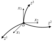
Figure 6.1: Cartesian and curvilinear coordinates.

Any point $p\in\mathcal{E}$ can be identified by either set of coordinates; mathematically, this means that there must be an isomorphism between the $x_{k}$s and the $z^{j}$s, i.e. invertible relations of the kind

$$\begin{array}[]{l}z^{j}=z^{j}(x_{1},x_{2},x_{3})=z^{j}(x_{k}),\vskip 6.0pt plus 2.0pt minus 2.0pt\\ x_{k}=x_{k}(z^{1},z^{2},z^{3})=x_{k}(z^{j}),\end{array}\ \ \ \ \forall j,k=1,2,3$$ (6.1)

exist between the two sets of coordinates. The distance between two points $p,q\in\mathcal{E}$ is

$$s=\sqrt{(p-q)\cdot(p-q)}=\sqrt{(x_{k}^{p}-x_{k}^{q})(x_{k}^{p}-x_{k}^{q})}$$

but this is no longer true for curvilinear coordinates:

$$s\neq\sqrt{({z^{j}}^{p}-{z^{j}}^{q})({z^{j}}^{p}-{z^{j}}^{q})}.$$

However, if $p\rightarrow q$, we can define

$$dx_{k}=x_{k}^{p}-x_{k}^{q},\ \ \ dz^{j}={z^{j}}^{p}-{z^{j}}^{q},$$

so using Eq. (6.1)₂

$$dx_{k}=\frac{\partial x_{k}}{\partial z^{j}}dz^{j}.$$ (6.2)

The (infinitesimal) distance between $p$ and $q$ will then be

$$ds=\sqrt{dx_{k}dx_{k}}=\sqrt{\frac{\partial x_{k}}{\partial z^{j}}\frac{\partial x_{k}}{\partial z^{l}}dz^{j}dz^{l}}=\sqrt{g_{jl}dz^{j}dz^{l}},$$

where

$$g_{jl}=g_{lj}=\frac{\partial x_{k}}{\partial z^{j}}\frac{\partial x_{k}}{\partial z^{l}}$$ (6.3)

are the covariant components of the metric tensor $\mathbf{g}\in Sym(\mathcal{V})$. We note that, as $\mathbf{g}$ defines a positive quadratic form (the square length of a vector), it is a positive definite symmetric tensor, so

$$\det\mathbf{g}>0.$$ (6.4)

Coming back to the vector notation, from Eq. (6.2) we get

$$dx=dx_{i}\mathbf{e}_{i}=\frac{\partial x_{i}}{\partial z^{k}}dz^{k}\mathbf{e}_{i};$$

introducing the vector $\mathbf{g}_{k}$,

$$\mathbf{g}_{k}:=\frac{\partial x_{i}}{\partial z^{k}}\mathbf{e}_{i},$$ (6.5)

we can write

$$dx=dz^{k}\mathbf{g}_{k}.$$

We see hence that a vector $dx$ can be expressed as a linear combination of the vectors $\mathbf{g}_{k}$; these form therefore a basis, called the local basis. Generally speaking, $\mathbf{g}_{k}\notin\mathcal{S}$ and it is clearly tangent to the lines $z^{j}=const$. This can be seen in Fig. 6.2 for a two-dimensional case:

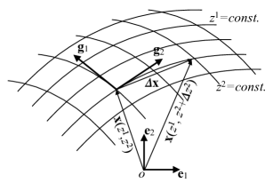
Figure 6.2: Tangent vectors to the curvilinear coordinates lines.

$$dx=\lim_{\Delta\mathbf{x}\rightarrow 0}\Delta\mathbf{x}=\lim_{\Delta\mathbf{x}\rightarrow 0}\frac{x_{i}(z^{1},z^{2}+\Delta z^{2})-x_{i}(z^{1},z^{2})}{\Delta z^{2}}\Delta z^{2}\mathbf{e}_{i}=\frac{\partial x_{i}}{\partial z^{2}}\mathbf{e}_{i}dz^{2}=\mathbf{g}_{2}dz^{2}.$$

Then

$$\mathbf{g}_{k}\cdot\mathbf{g}_{l}=\frac{\partial x_{i}}{\partial z^{k}}\mathbf{e}_{i}\cdot\frac{\partial x_{j}}{\partial z^{l}}\mathbf{e}_{j}=\frac{\partial x_{i}}{\partial z^{k}}\frac{\partial x_{j}}{\partial z^{l}}\delta_{ij}=g_{kl},$$ (6.6)

i.e. the components of the metric tensor $\mathbf{g}$ are the scalar products of the tangent vectors $\mathbf{g}_{k}$s. If the curvilinear coordinates are orthogonal, i.e. if $\mathbf{g}_{h}\cdot\mathbf{g}_{k}=0\ \forall h,k=1,2,3,h\neq k$, then $\mathbf{g}$ is diagonal. If, in addition, $\mathbf{g}_{k}\in\mathcal{S}\ \forall k=1,2,3$, then $\mathbf{g}=\mathbf{I}$: It is the case of Cartesian coordinates. As an example, let us consider the case of polar coordinates,

$$\left\{\begin{array}[]{l}x_{1}=r\ \cos\theta,\\ x_{2}=r\ \sin\theta,\end{array}\right.\ \ \ \left\{\begin{array}[]{l}z^{1}=r=\sqrt{x_{1}^{2}+x_{2}^{2}},\\ z^{2}=\theta=\arctan\dfrac{x_{2}}{x_{1}}.\end{array}\right.$$

Hence, see Fig. 6.3,

$$\begin{split}&\mathbf{g}_{1}=\frac{\partial x_{1}}{\partial z^{1}}\mathbf{e}_{1}+\frac{\partial x_{2}}{\partial z^{1}}\mathbf{e}_{2}=\cos\theta\mathbf{e}_{1}+\sin\theta\mathbf{e}_{2}=\mathbf{e}_{r},\\ &\mathbf{g}_{2}=\frac{\partial x_{1}}{\partial z^{2}}\mathbf{e}_{1}+\frac{\partial x_{2}}{\partial z^{2}}\mathbf{e}_{2}=-r\sin\theta\mathbf{e}_{1}+r\cos\theta\mathbf{e}_{2}=r\mathbf{e}_{\theta}.\end{split}$$

We remark that $|\mathbf{g}_{1}|=1$ but $|\mathbf{g}_{2}|\neq 1$ and it is variable with the position.

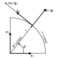
Figure 6.3: Tangent vectors to the polar coordinates lines.

6.3 Co- and contra-variant components

A geometrical way to introduce the concept of covariant and contravariant components is to consider how to represent a vector $\mathbf{v}$ in the $z-$system. There are basically two ways, cf. Fig. 6.4, referred, for the sake of simplicity, to a planar case:

1. contravariant components: $\mathbf{v}$ is projected parallel to $z^{1}$ and $z^{2}$; they are indicated by superscripts: $\mathbf{v}=(v^{1},v^{2},v^{3})$;

2. covariant components: $\mathbf{v}$ is projected perpendicularly to $z^{1}$ and $z^{2}$; they are indicated by subscripts: $\mathbf{v}=(v_{1},v_{2},v_{3})$;

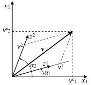
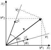
Figure 6.4: Contravariant (left) and covariant (right) components of a vector in a plane.

Still referring to the planar case in Fig. 6.4, if the Cartesian components of $\mathbf{v}$ are $\mathbf{v}=(v^{c}_{1},v^{c}_{2})$, we get

$$\left\{\begin{array}[]{l}v^{1}=h(v_{1}^{c}\sin\alpha_{2}-v_{2}^{c}\cos\alpha_{2}),\\ v^{2}=h(-v_{1}^{c}\sin\alpha_{1}+v_{2}^{c}\cos\alpha_{1}),\end{array}\right.\ \ \ \left\{\begin{array}[]{l}v_{1}=v_{1}^{c}\cos\alpha_{1}+v_{2}^{c}\sin\alpha_{1},\\ v_{2}=v_{1}^{c}\cos\alpha_{2}+v_{2}^{c}\sin\alpha_{2},\end{array}\right.$$ (6.7)

and conversely

$$\left\{\begin{array}[]{l}v^{c}_{1}=v^{1}\cos\alpha_{1}+v^{2}\cos\alpha_{2},\\ v^{c}_{2}=v^{1}\sin\alpha_{1}+v^{2}\sin\alpha_{2},\end{array}\right.\ \ \ \left\{\begin{array}[]{l}v_{1}^{c}=h(v_{1}\sin\alpha_{2}-v_{2}\sin\alpha_{1}),\\ v^{c}_{2}=h(-v_{1}\cos\alpha_{2}+v_{2}\cos\alpha_{1}),\end{array}\right.$$ (6.8)

with

$$h=\frac{1}{\sin(\alpha_{2}-\alpha_{1})}.$$

It is apparent that the Cartesian coordinates are at the same time co- and contra-variant. Still on a planar scheme, we can see how to pass from a system of coordinates to another one, cf. Fig. 6.5.

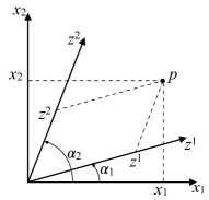
Figure 6.5: Relation between Cartesian and contravariant components.

For a point $p$ the Cartesian coordinates $(x_{1},x_{2})$ are related to the contravariant ones by

$$\begin{split}&x_{1}=z^{1}\cos\alpha_{1}+z^{2}\cos\alpha_{2},\\ &x_{2}=z^{1}\sin\alpha_{1}+z^{2}\sin\alpha_{2},\end{split}$$

and, conversely,

$$\begin{split}&z^{1}=h(x_{1}\sin\alpha_{2}-x_{2}\cos\alpha_{2}),\\ &z^{2}=h(-x_{1}\sin\alpha_{1}+x_{2}\cos\alpha_{1}).\end{split}$$

So, differentiating, we get

$$\begin{split}&\frac{\partial x_{1}}{\partial z^{1}}=\cos\alpha_{1},\ \frac{\partial x_{1}}{\partial z^{2}}=\cos\alpha_{2},\\ &\frac{\partial x_{2}}{\partial z^{1}}=\sin\alpha_{1},\ \frac{\partial x_{2}}{\partial z^{2}}=\sin\alpha_{2},\\ \end{split}$$

and

$$\begin{split}&\frac{\partial z^{1}}{\partial x_{1}}=h\sin\alpha_{2},\ \frac{\partial z^{1}}{\partial x_{2}}=-h\cos\alpha_{2},\\ &\frac{\partial z^{2}}{\partial x_{1}}=-h\sin\alpha_{1},\ \frac{\partial z^{2}}{\partial x_{2}}=h\cos\alpha_{1}.\\ \end{split}$$

Injecting these expressions into Eqs. (6.7) and (6.8) gives

$$\begin{split}&v_{1}=v_{1}^{c}\frac{\partial x_{1}}{\partial z^{1}}+v_{2}^{c}\frac{\partial x_{2}}{\partial z^{1}},\\ &v_{2}=v_{1}^{c}\frac{\partial x_{1}}{\partial z^{2}}+v_{2}^{c}\frac{\partial x_{2}}{\partial z^{2}},\end{split}\ \rightarrow\ v_{i}=\frac{\partial x_{k}}{\partial z^{i}}v_{k}^{c}$$ (6.9)

and

$$\begin{split}&v^{1}=v_{1}^{c}\frac{\partial z^{1}}{\partial x_{1}}+v_{2}^{c}\frac{\partial z^{1}}{\partial x_{2}},\\ &v^{2}=v_{1}^{c}\frac{\partial z^{2}}{\partial x_{1}}+v_{2}^{c}\frac{\partial z^{2}}{\partial x_{2}},\end{split}\ \rightarrow\ v^{i}=\frac{\partial z^{i}}{\partial x_{k}}v_{k}^{c}.$$ (6.10)

Now, if we calculate

$$g_{hi}v^{i}=g_{hi}\frac{\partial z^{i}}{\partial x_{k}}v_{k}^{c},$$

from Eq. (6.3) and by the chain rule we get

$$\begin{split}g_{hi}v^{i}&=\frac{\partial x_{j}}{\partial z^{h}}\frac{\partial x_{j}}{\partial z^{i}}\frac{\partial z^{i}}{\partial x_{k}}v_{k}^{c}\\ &=\frac{\partial x_{j}}{\partial z^{h}}\frac{\partial x_{j}}{\partial x_{k}}v_{k}^{c}=\frac{\partial x_{j}}{\partial z^{h}}\delta_{jk}v_{k}^{c}=\frac{\partial x_{k}}{\partial z^{h}}v_{k}^{c}=v_{h},\end{split}$$

i.e. we obtain the rule of lowering of the indices for passing from contravariant to covariant components:

$$v_{h}=g_{hi}v^{i}.$$

Introducing the inverse to $g_{hi}$ as

$$g^{hi}=\frac{\partial z^{h}}{\partial x_{k}}\frac{\partial z^{i}}{\partial x_{k}},$$ (6.11)

we get, still using the chain rule,

$$\begin{split}g^{hi}v_{i}&=g^{hi}\frac{\partial x_{k}}{\partial z^{i}}v_{k}^{c}=\frac{\partial z^{h}}{\partial x_{j}}\frac{\partial z^{i}}{\partial x_{j}}\frac{\partial x_{k}}{\partial z^{i}}v_{k}^{c}\\ &=\frac{\partial z^{h}}{\partial x_{j}}\frac{\partial x_{k}}{\partial x_{j}}v_{k}^{c}=\frac{\partial z^{h}}{\partial x_{j}}\delta_{jk}v_{k}^{c}=\frac{\partial z^{h}}{\partial x_{k}}v_{k}^{c}=v^{h},\end{split}$$

which is the rule of raising of the indices for passing from covariant to contravariant components:

$$v^{h}=g^{hi}v_{i}.$$

Again applying the chain rule, by Eq. (6.9) we get

$$\frac{\partial z^{i}}{\partial x_{l}}v_{i}=\frac{\partial z^{i}}{\partial x_{l}}\frac{\partial x_{k}}{\partial z^{i}}v_{k}^{c}=\frac{\partial x_{k}}{\partial x_{l}}v_{k}^{c}=\delta_{kl}v_{k}^{c},$$

i.e.

$$v_{k}^{c}=\frac{\partial z^{i}}{\partial x_{k}}v_{i},$$ (6.12)

which is the converse of Eq. (6.9). In a similar way, we get the converse of Eq. (6.10):

$$v_{k}^{c}=\frac{\partial x_{k}}{\partial z^{i}}v^{i}.$$ (6.13)

Let us now calculate the norm $v$ of a vector $\mathbf{v}$; starting from the Cartesian components and using the last two results,

$$v=\sqrt{\mathbf{v}\cdot\mathbf{v}}=\sqrt{v_{k}^{c}v_{k}^{c}}=\sqrt{\frac{\partial z^{i}}{\partial x_{k}}v_{i}\frac{\partial z^{j}}{\partial x_{k}}v_{j}}=\sqrt{\frac{\partial z^{i}}{\partial x_{k}}\frac{\partial z^{j}}{\partial x_{k}}v_{i}v_{j}}=\sqrt{g^{ij}v_{i}v_{j}},$$

or also

$$v=\sqrt{\mathbf{v}\cdot\mathbf{v}}=\sqrt{v_{k}^{c}v_{k}^{c}}=\sqrt{\frac{\partial x_{k}}{\partial z^{i}}v^{i}\frac{\partial x_{k}}{\partial z^{j}}v^{j}}=\sqrt{\frac{\partial x_{k}}{\partial z^{i}}\frac{\partial x_{k}}{\partial z^{j}}v^{i}v^{j}}=\sqrt{g_{ij}v^{i}v^{j}}$$

and even

$$v=\sqrt{\mathbf{v}\cdot\mathbf{v}}=\sqrt{v_{k}^{c}v_{k}^{c}}=\sqrt{\frac{\partial z^{i}}{\partial x_{k}}v_{i}\frac{\partial x_{k}}{\partial z^{j}}v^{j}}=\sqrt{\frac{\partial z^{i}}{\partial x_{k}}\frac{\partial x_{k}}{\partial z^{j}}v_{i}v^{j}}=\sqrt{\delta^{i}_{\ j}v_{i}v^{j}}=\sqrt{v_{i}v^{i}}.$$

Through Eq. (6.13) and by the definition of the tangent vectors to the lines of curvilinear coordinates, Eq. (6.5), for a vector $\mathbf{v}$ we get

$$\mathbf{v}=v_{i}^{c}\mathbf{e}_{i}=v^{k}\frac{\partial x_{i}}{\partial z^{k}}\mathbf{e}_{i}=v^{k}\mathbf{g}_{k}.$$

We see hence that the contravariant components are actually the components of $\mathbf{v}$ in the local basis, composed by vectors $\mathbf{g}_{k}$s, tangent to the lines of curvilinear coordinates. In a similar manner, if we introduce the dual basis whose vectors $\mathbf{g}^{k}$ are defined as

$$\mathbf{g}^{k}:=\frac{\partial z^{k}}{\partial x_{i}}\mathbf{e}_{i}$$ (6.14)

and proceeding in the same way, we obtain that

$$\mathbf{v}=v_{i}^{c}\mathbf{e}_{i}=v_{k}\frac{\partial z^{k}}{\partial x_{i}}\mathbf{e}_{i}=v_{k}\mathbf{g}^{k},$$

i.e. the covariant components are actually the components of $\mathbf{v}$ in the dual basis. Finally, for a vector, we have, alternatively,

$$\mathbf{v}=v_{i}^{c}\mathbf{e}_{i}=v^{k}\mathbf{g}_{k}=v_{k}\mathbf{g}^{k}.$$ (6.15)

Just as for the $\mathbf{g}_{k}$s, we have

$$\mathbf{g}^{h}\cdot\mathbf{g}^{k}=\left(\frac{\partial z^{h}}{\partial x_{i}}\mathbf{e}_{i}\right)\cdot\left(\frac{\partial z^{k}}{\partial x_{j}}\mathbf{e}_{j}\right)=\frac{\partial z^{h}}{\partial x_{i}}\frac{\partial z^{k}}{\partial x_{j}}\delta_{ij}=\frac{\partial z^{h}}{\partial x_{i}}\frac{\partial z^{k}}{\partial x_{i}}=g^{hk};$$

moreover

$$\mathbf{g}^{h}\cdot\mathbf{g}_{k}=\left(\frac{\partial z^{h}}{\partial x_{i}}\mathbf{e}_{i}\right)\cdot\left(\frac{\partial x_{j}}{\partial z^{k}}\mathbf{e}_{j}\right)=\frac{\partial z^{h}}{\partial x_{i}}\frac{\partial x_{j}}{\partial z^{k}}\delta_{ij}=\frac{\partial z^{h}}{\partial x_{i}}\frac{\partial x_{i}}{\partial z^{k}}=\frac{\partial z^{h}}{\partial z^{k}}=\delta^{h}_{\ k},$$

and, by the symmetry of the scalar product,

$$\delta_{h}^{\ k}:=\mathbf{g}_{h}\cdot\mathbf{g}^{k}=\mathbf{g}^{k}\cdot\mathbf{g}_{h}=\delta^{k}_{\ h}.$$

The last equations defines the orthogonality conditions for the $\mathbf{g}$-vectors. Using these results and Eq. (6.15) we also have

$$\begin{split}&v^{k}=\delta_{\ h}^{k}v^{h}=\mathbf{g}^{k}\cdot v^{h}\mathbf{g}_{h}=\mathbf{g}^{k}\cdot\mathbf{v}=\mathbf{g}^{k}\cdot v_{h}\mathbf{g}^{h}=g^{kh}v_{h},\\ &v_{k}=\delta_{k}^{\ h}v_{h}=\mathbf{g}_{k}\cdot v_{h}\mathbf{g}^{h}=\mathbf{g}_{k}\cdot\mathbf{v}=\mathbf{g}_{k}\cdot v^{h}\mathbf{g}_{h}=g_{kh}v^{h},\end{split}$$

thus finding again the rules of raising and lowering of the indices.

What was done for vectors can be transposed, using a similar approach, to tensors. In particular, for a second-rank tensor $\mathbf{L}$, we get

$$\begin{split}&L^{ij}=\frac{\partial z^{i}}{\partial x_{h}}\frac{\partial z^{j}}{\partial x_{k}}L_{hk}^{c},\\ &L_{ij}=\frac{\partial x_{h}}{\partial z^{i}}\frac{\partial x_{k}}{\partial z^{j}}L_{hk}^{c},\end{split}$$ (6.16)

for the contravariant and covariant components, respectively, while we can also introduce the mixed components

$$\begin{split}&L^{i}_{\ j}=\frac{\partial z^{i}}{\partial x_{h}}\frac{\partial x_{k}}{\partial z^{j}}L_{hk}^{c},\\ &L_{i}^{\ j}=\frac{\partial x_{h}}{\partial z^{i}}\frac{\partial z^{j}}{\partial x_{k}}L_{hk}^{c}.\end{split}$$ (6.17)

Conversely,

$$\begin{split}&L_{hk}^{c}=\frac{\partial x_{h}}{\partial z^{i}}\frac{\partial x_{k}}{\partial z^{j}}L^{ij},\\ &L_{hk}^{c}=\frac{\partial z^{i}}{\partial x_{h}}\frac{\partial z^{j}}{\partial x_{k}}L_{ij},\\ &L_{hk}^{c}=\frac{\partial x_{h}}{\partial z^{i}}\frac{\partial z^{j}}{\partial x_{k}}L^{i}_{\ j},\\ &L_{hk}^{c}=\frac{\partial z^{i}}{\partial x_{h}}\frac{\partial x_{k}}{\partial z^{j}}L_{i}^{\ j}.\end{split}$$ (6.18)

Also for $\mathbf{L}$, the rule of lowering or raising the indices is valid:

$$L^{ij}=g^{ih}g^{jk}L_{hk},\ \ \ L_{ij}=g_{ih}g_{jk}L^{hk}.$$ (6.19)

From Eq. (6.18) and by the same definitions of $g_{ij}$, eq.(6.3), and $g^{ij}$, Eq. (6.11), we get

$$\mathbf{L}=L_{ij}^{c}\mathbf{e}_{i}\otimes\mathbf{e}_{j}=\frac{\partial x_{i}}{\partial z^{h}}\frac{\partial x_{j}}{\partial z^{k}}L^{hk}\mathbf{e}_{i}\otimes\mathbf{e}_{j}=L^{hk}\mathbf{g}_{h}\otimes\mathbf{g}_{k}$$

and

$$\mathbf{L}=L_{ij}^{c}\mathbf{e}_{i}\otimes\mathbf{e}_{j}=\frac{\partial z^{h}}{\partial x_{i}}\frac{\partial z^{k}}{\partial x_{j}}L_{hk}\mathbf{e}_{i}\otimes\mathbf{e}_{j}=L_{hk}\mathbf{g}^{h}\otimes\mathbf{g}^{k}.$$

In a similar manner, the tensor mixed components are also found:

$$\mathbf{L}=L_{ij}^{c}\mathbf{e}_{i}\otimes\mathbf{e}_{j}=\frac{\partial x_{i}}{\partial z^{h}}\frac{\partial z^{k}}{\partial x_{j}}L^{h}_{\ k}\mathbf{e}_{i}\otimes\mathbf{e}_{j}=L^{h}_{\ k}\mathbf{g}_{h}\otimes\mathbf{g}^{k}$$

and

$$\mathbf{L}=L_{ij}^{c}\mathbf{e}_{i}\otimes\mathbf{e}_{j}=\frac{\partial z^{k}}{\partial x_{j}}\frac{\partial x_{i}}{\partial z^{h}}L_{h}^{\ k}\mathbf{e}_{i}\otimes\mathbf{e}_{j}=L_{h}^{\ k}\mathbf{g}^{h}\otimes\mathbf{g}_{k}.$$

We see hence that a second-rank tensor can be given with four different combinations of coordinates; even more complex is the case of higher order tensors, which will not be treated here.

Still by eqs.(6.3) and (6.11) and applying the chain rule to $\delta^{i}_{j}=\dfrac{\partial z^{i}}{\partial z^{j}}$, we get

$$\begin{split}&g_{ij}=\frac{\partial x_{k}}{\partial z^{i}}\frac{\partial x_{k}}{\partial z^{j}}=\frac{\partial x_{h}}{\partial z^{i}}\frac{\partial x_{k}}{\partial z^{j}}\delta_{hk},\\ &g^{ij}=\frac{\partial z^{i}}{\partial x_{k}}\frac{\partial z^{j}}{\partial x_{k}}=\frac{\partial z^{i}}{\partial x_{h}}\frac{\partial z^{j}}{\partial x_{k}}\delta_{hk},\\ &\delta^{i}_{\ j}=\frac{\partial z^{i}}{\partial x_{h}}\frac{\partial x_{k}}{\partial z^{j}}\delta_{hk},\\ &\delta_{i}^{\ j}=\frac{\partial x_{h}}{\partial z^{i}}\frac{\partial z^{j}}{\partial x_{k}}\delta_{hk}.\end{split}$$ (6.20)

So, applying Eq. (6.18) to the identity tensor, we get

$$\mathbf{I}=\delta_{ij}\mathbf{e}_{i}\otimes\mathbf{e}_{j}=\frac{\partial x_{i}}{\partial z^{h}}\frac{\partial x_{j}}{\partial z^{k}}I^{hk}\mathbf{e}_{i}\otimes\mathbf{e}_{j}=I^{hk}\mathbf{g}_{h}\otimes\mathbf{g}_{k},$$

but by Eqs. (6.16) and (6.20),

$$I^{hk}=\frac{\partial z^{h}}{\partial x_{i}}\frac{\partial z^{k}}{\partial x_{j}}\delta_{ij}=g^{hk}$$

so, finally,

$$\mathbf{I}=g^{hk}\mathbf{g}_{h}\otimes\mathbf{g}_{k}.$$

Proceeding in a similar manner, we can also get

$$\mathbf{I}=g_{hk}\mathbf{g}^{h}\otimes\mathbf{g}^{k}=\delta^{h}_{\ k}\mathbf{g}_{h}\otimes\mathbf{g}^{k}=\delta_{h}^{\ k}\mathbf{g}^{h}\otimes\mathbf{g}_{k}.$$

We see hence that the $g_{hk}$s represent $\mathbf{I}$ in covariant coordinates, the $g^{hk}$s in the contravariant ones and the $\delta_{h}^{\ k}$s and $\delta^{h}_{\ k}$s in mixed coordinates.

6.4 Spatial derivatives of fields in curvilinear coordinates

Let $\varphi$ a spatial scalar field, $\varphi:\mathcal{E}\rightarrow\mathbb{R}$. Generally speaking,

$$\varphi=\varphi(z^{j}(x_{i})),$$

or also

$$\varphi=\varphi(x_{j}(z^{k})),$$

where the $x_{j}$s, $z^{k}$s are, respectively, Cartesian and curvilinear coordinates, related as in Eq. (6.1). By the chain rule

$$\frac{\partial\varphi}{\partial x_{j}}=\frac{\partial\varphi}{\partial z^{k}}\frac{\partial z^{k}}{\partial x_{j}}$$ (6.21)

and inversely

$$\frac{\partial\varphi}{\partial z^{k}}=\frac{\partial\varphi}{\partial x_{j}}\frac{\partial x_{j}}{\partial z^{k}}.$$

We remark that the last quantity transforms like the components of a covariant vector, cf. Eq. (6.9).

The gradient of $\varphi$ is the vector that in the Cartesian basis, cf. Eq. (5.6)₁, is given by

$$\nabla\varphi=\frac{\partial\varphi}{\partial x_{j}}\mathbf{e}_{j};$$

so by Eqs. (6.14) and (6.21) we get that, in the dual basis,

$$\nabla\varphi=\frac{\partial\varphi}{\partial z^{k}}\frac{\partial z^{k}}{\partial x_{j}}\mathbf{e}_{j}=\frac{\partial\varphi}{\partial z^{k}}\mathbf{g}^{k}.$$

We see hence that in curvilinear coordinates the nabla operator, Eq. (5.7), is defined by

$$\nabla(\cdot)=\frac{\partial\ \cdot}{\partial z^{k}}\mathbf{g}^{k}.$$ (6.22)

The contravariant components of the gradient can be obtained by the covariant ones upon multiplication by the components of the inverse (contravariant) metric tensor, Eq. (6.11):

$$g^{hk}\frac{\partial\varphi}{\partial z^{k}}=\frac{\partial z^{h}}{\partial x_{i}}\frac{\partial z^{k}}{\partial x_{i}}\frac{\partial\varphi}{\partial x_{j}}\frac{\partial x_{j}}{\partial z^{k}}=\delta_{ij}\frac{\partial\varphi}{\partial x_{j}}\frac{\partial z^{h}}{\partial x_{i}}=\frac{\partial\varphi}{\partial x_{j}}\frac{\partial z^{h}}{\partial x_{j}}\ \rightarrow\ \nabla\varphi=\frac{\partial\varphi}{\partial x_{j}}\frac{\partial z^{h}}{\partial x_{j}}\mathbf{g}_{h}.$$

Let us now consider a vector field $\mathbf{v}:\mathcal{E}\rightarrow\mathcal{V}$; we want to calculate the spatial derivative of its Cartesian components. By the chain rule and Eq. (6.13), we get

$$\begin{split}\frac{\partial v_{i}^{c}}{\partial x_{j}}&=\frac{\partial v_{i}^{c}}{\partial z^{k}}\frac{\partial z^{k}}{\partial x_{j}}=\frac{\partial z^{k}}{\partial x_{j}}\frac{\partial}{\partial z^{k}}\left(\frac{\partial x_{i}}{\partial z^{h}}v^{h}\right)=\frac{\partial z^{k}}{\partial x_{j}}\left(\frac{\partial x_{i}}{\partial z^{h}}\frac{\partial v^{h}}{\partial z^{k}}+\frac{\partial^{2}x_{i}}{\partial z^{k}\partial z^{l}}v^{l}\right)\\ &=\frac{\partial z^{k}}{\partial x_{j}}\frac{\partial x_{i}}{\partial z^{h}}\left(\frac{\partial v^{h}}{\partial z^{k}}+\frac{\partial z^{h}}{\partial x_{m}}\frac{\partial^{2}x_{m}}{\partial z^{k}\partial z^{l}}v^{l}\right),\end{split}$$

whence

$$\frac{\partial z^{h}}{\partial x_{i}}\frac{\partial x_{j}}{\partial z^{k}}\frac{\partial v_{i}^{c}}{\partial x_{j}}=\frac{\partial v^{h}}{\partial z^{k}}+\frac{\partial z^{h}}{\partial x_{m}}\frac{\partial^{2}x_{m}}{\partial z^{k}\partial z^{l}}v^{l}.$$ (6.23)

Comparing this result with Eq. (6.17)₁ we see that the first member actually corresponds to the components of a mixed tensor field, which is the gradient of the vector field $\mathbf{v}$, that we write as

$$v^{h}_{\ ;k}=\frac{\partial v^{h}}{\partial z^{k}}+\Gamma^{h}_{kl}v^{l},$$ (6.24)

where the functions

$$\Gamma^{h}_{kl}=\frac{\partial z^{h}}{\partial x_{m}}\frac{\partial^{2}x_{m}}{\partial z^{k}\partial z^{l}}$$ (6.25)

are the Christoffel symbols. We immediately see that $\Gamma^{h}_{kl}=\Gamma^{h}_{lk}$. The quantity $v^{h}_{\ ;k}$ is the covariant derivative of the contravariant components $v^{h}$. The proof that the Christoffel symbols can also be written as

$$\Gamma^{h}_{kl}=\frac{1}{2}g^{hm}\left(\frac{\partial g_{mk}}{\partial z^{l}}+\frac{\partial g_{ml}}{\partial z^{k}}-\frac{\partial g_{kl}}{\partial z^{m}}\right)$$ (6.26)

is left to the reader as an exercise.

Proceeding in a similar way for the covariant components of $\mathbf{v}$, but now using Eqs. (6.12) and (6.17)₁, we get

$$v_{h;k}=\frac{\partial v_{h}}{\partial z^{k}}-\Gamma^{l}_{kh}v_{l},$$

which is the covariant derivative of the covariant components $v_{h}$.

Using Eqs. (6.23) and (6.24), we conclude that, cf. Eq. (5.6)₃,

$$\mathrm{div}\mathbf{v}=\frac{\partial v^{c}_{i}}{\partial x_{i}}=v^{h}_{\ ;h}.$$

Then, applying the operator divergence so defined to the gradient of the scalar field $\varphi$ we obtain, in curvilinear coordinates $z^{k}$, the Laplacian $\Delta\varphi$ as

$$\Delta\varphi=\left(g^{hk}\frac{\partial\varphi}{\partial z^{k}}\right)_{;h}=\frac{\partial}{\partial z^{h}}\left(g^{hk}\frac{\partial\varphi}{\partial z^{k}}\right)+\Gamma^{h}_{hj}g^{jk}\frac{\partial\varphi}{\partial z^{k}}.$$ (6.27)

Using the definition of the nabla operator in curvilinear coordinates, Eq. (6.22), jointly to the fact that, cf. Section 5.5,

$$\Delta f:=\mathrm{div}\nabla\varphi=\nabla\cdot\nabla\varphi,$$

we get the the following representation of the Laplace operator in curvilinear coordinates:

$$\begin{split}\Delta(\cdot)&=\nabla\cdot\nabla(\cdot)=\left(\frac{\partial}{\partial z^{k}}\left(\frac{\partial(\cdot)}{\partial z^{h}}\mathbf{g}^{h}\right)\right)\cdot\mathbf{g}^{k}=\frac{\partial^{2}(\cdot)}{\partial z^{k}\partial z^{h}}\mathbf{g}^{h}\cdot\mathbf{g}^{k}+\frac{\partial\mathbf{g}^{h}}{\partial z^{k}}\frac{\partial(\cdot)}{\partial z^{h}}\cdot\mathbf{g}^{k}\\ &=\frac{\partial^{2}(\cdot)}{\partial z^{k}\partial z^{h}}g^{hk}+\frac{\partial\mathbf{g}^{h}}{\partial z^{k}}\cdot\mathbf{g}^{k}\frac{\partial(\cdot)}{\partial z^{h}}.\end{split}$$

Let us now calculate the spatial derivatives of the components of a 2^nd-rank tensor $\mathbf{L}$: By Eqs. (6.18)₁ and (6.25) we get

$$\begin{split}\frac{\partial L_{ij}^{c}}{\partial x_{k}}&=\frac{\partial z^{h}}{\partial x_{k}}\frac{\partial}{\partial z^{h}}\left(\frac{\partial x_{i}}{\partial z^{n}}\frac{\partial x_{j}}{\partial z^{p}}L^{np}\right)\\ &=\frac{\partial z^{h}}{\partial x_{k}}\frac{\partial x_{i}}{\partial z^{n}}\frac{\partial x_{j}}{\partial z^{p}}\left(\frac{\partial L^{np}}{\partial z^{h}}+\Gamma_{hr}^{n}L^{rp}+\Gamma_{hr}^{p}L^{nr}\right),\end{split}$$

which implies that

$$\frac{\partial L^{np}}{\partial z^{h}}+\Gamma_{hr}^{n}L^{rp}+\Gamma_{hr}^{p}L^{nr}=\frac{\partial x_{k}}{\partial z^{h}}\frac{\partial z^{n}}{\partial x_{i}}\frac{\partial z^{p}}{\partial x_{j}}\frac{\partial L_{ij}^{c}}{\partial x_{k}}.$$ (6.28)

So, using Eq. (6.16), we can conclude that the expression

$$L^{np}_{\ \ ;h}=\frac{\partial L^{np}}{\partial z^{h}}+\Gamma_{hr}^{n}L^{rp}+\Gamma_{hr}^{p}L^{nr}$$ (6.29)

represents the covariant derivative of the contravariant components of the second-rank tensor $\mathbf{L}$. In a similar manner, this time by Eq. (6.18)₂, we obtain the covariant derivatives of the covariant components of $\mathbf{L}$:

$$\frac{\partial L_{np}}{\partial z^{h}}-\Gamma_{nh}^{r}L_{rp}-\Gamma_{ph}^{r}L_{nr}=\frac{\partial x_{k}}{\partial z^{h}}\frac{\partial x_{i}}{\partial z^{n}}\frac{\partial x_{j}}{\partial z^{p}}\frac{\partial L_{ij}^{c}}{\partial x_{k}},$$

i.e.

$$L_{np;h}=\frac{\partial L_{np}}{\partial z^{h}}-\Gamma_{ph}^{r}L_{nr}-\Gamma_{nh}^{r}L_{pr}.$$ (6.30)

The same procedure with Eqs. (6.18)_3,4 gives the covariant derivatives of the mixed components of $\mathbf{L}$:

$$\begin{split}L^{n}_{\ p;h}=\frac{\partial L^{n}_{\ p}}{\partial z^{h}}+\Gamma_{hr}^{n}L^{r}_{\ p}-\Gamma_{ph}^{r}L^{n}_{\ r},\\ L_{p\ ;h}^{\ n}=\frac{\partial L^{\ n}_{p}}{\partial z^{h}}-\Gamma_{ph}^{r}L_{r}^{\ n}+\Gamma_{hr}^{n}L_{p}^{\ r}.\end{split}$$ (6.31)

If in Eqs. (6.28) and (6.29) we set $p=h$, we get

$$\begin{split}L^{nh}_{\ \ ;h}&=\frac{\partial L^{nh}}{\partial z^{h}}+\Gamma_{hr}^{n}L^{rh}+\Gamma_{hr}^{h}L^{nr}=\frac{\partial x_{k}}{\partial z^{h}}\frac{\partial z^{n}}{\partial x_{i}}\frac{\partial z^{h}}{\partial x_{j}}\frac{\partial L_{ij}^{c}}{\partial x_{k}}\\ &=\delta_{kj}\frac{\partial z^{n}}{\partial x_{i}}\frac{\partial L_{ij}^{c}}{\partial x_{k}}=\frac{\partial z^{n}}{\partial x_{i}}\frac{\partial L_{ij}^{c}}{\partial x_{j}},\end{split}$$

which are the components of the contravariant vector field $\mathrm{div}\mathbf{L}$.

6.5 Exercises

1. Write $\mathbf{g}$ and $ds$ for cylindrical coordinates.

2. Write $\mathbf{g}$ and $ds$ for spherical coordinates.

3. Find the length of a helix traced on a circular cylinder of radius $R$ between the angles $\theta$ and $\theta+2\pi$.

4. A curve is traced in a quarter circle of radius $R$, see Fig. 6.6, with $\rho$ proportional to $\theta$. When the quarter of circle is rolled into a cone, the curve appears as indicated in the figure. Determine the length $\ell$ of the curve, first using the polar coordinates in the plane of the quarter circle, then the cylindrical ones for the case of the curve on the cone (exercise given in the book by W. H. Müller, see the suggested texts).

   

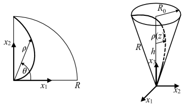
   Figure 6.6: Curve in a plane and on a cone.

5. Calculate $\mathbf{g}$ for a planar system of coordinates composed of two axes $z^{1}$ and $z^{2}$ inclined, respectively, at $\alpha_{1}$ and $\alpha_{2}$ on the axis $x_{1}$. Then, find the vectors $\mathbf{g}_{k}$ and $\mathbf{g}^{k},\ k=1,2$, check the orthogonality conditions $\mathbf{g}^{h}\cdot\mathbf{g}_{k}=\delta^{h}_{\ k}$, determine the norm of these vectors and design them.

6. Calculate the $\mathbf{g}_{i}$s for a system of spherical coordinates.

7. In the plane, elliptical coordinates are defined by the relations

   $$x_{1}=c\ \cosh z^{1}\cos z^{2},\ \ x_{2}=c\ \sinh z^{1}\sin z^{2},\ \ z^{1}\in(0,\infty),\ z^{2}\in[0,2\pi);$$

   show that the lines $z^{1}=const.$ and $\ z^{2}=const.$ are confocal ellipses and hyperbolae, determine the axes of the ellipses in terms of the parameter $c$, discuss the limit case of ellipses that degenerate into a crack and determine its length. Finally, find $\mathbf{g},\mathbf{g}_{1}$ and $\mathbf{g}_{2}$.

8. Determine the co- and contravariant components of a tensor $\mathbf{L}$ in cylindrical coordinates.

9. Determine the co- and contravariant components of a tensor $\mathbf{L}$ in spherical coordinates.

10. Show that

    $$\mathrm{tr}\mathbf{L}=L_{ii}^{c}=g_{ij}L^{ij}=g^{ij}L_{ij}=L^{i}_{\ i}=L_{j}^{\ j}.$$

11. Prove Eq. (6.26).

12. Prove the Lemma of Ricci:

    $$\frac{\partial g_{jk}}{\partial z^{h}}=\Gamma^{i}_{jh}g_{ik}+\Gamma^{i}_{kh}g_{ji}.$$

13. Using Eq. (6.26), find the Christoffel symbols for the cylindrical, spherical and elliptical (in the plane) coordinates.

14. Write the Laplacian $\Delta f$ of a spatial scalar field $f$ in cylindrical and spherical coordinates.

15. Prove that

    $$g^{np}_{\ \ ;h}=g_{np;h}=0.$$

Chapter 7 Surfaces in $\mathcal{E}$

7.1 Surfaces in $\mathcal{E}$, coordinate lines, tangent planes

A function $\mathbf{f}(u,v):\Omega\subset\mathbb{R}^{2}\rightarrow\mathcal{E}$ of class $\geq$C¹ and such that its Jacobian

$$J=\left[\begin{array}[]{cc}\dfrac{\partial f_{1}}{\partial u}&\dfrac{\partial f_{1}}{\partial v}\vskip 6.0pt plus 2.0pt minus 2.0pt\\ \dfrac{\partial f_{2}}{\partial u}&\dfrac{\partial f_{2}}{\partial v}\vskip 6.0pt plus 2.0pt minus 2.0pt\\ \dfrac{\partial f_{3}}{\partial u}&\dfrac{\partial f_{3}}{\partial v}\end{array}\right]$$

has maximum rank (rank[J]=2) defines a surface in $\mathcal{E}$, see Fig. 7.1. We say also that $\mathbf{f}$ is an immersion of $\Omega$ into $\mathcal{E}$ and that the subset $\Sigma\subset\mathcal{E}$ image of $\mathbf{f}$ is the support or trace of the surface $\mathbf{f}$.

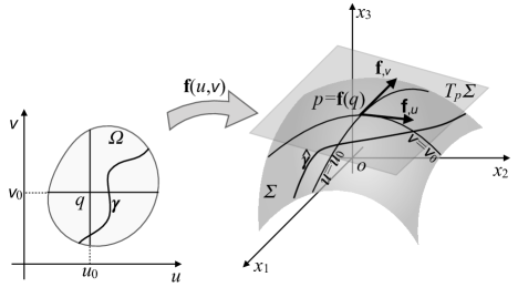
Figure 7.1: General scheme of a surface and of the tangent space at a point $p$.

As usual, we indicate the derivatives with respect to the variables $u,v$ by, for example, $\dfrac{\partial\mathbf{f}}{\partial u}=\mathbf{f}_{,u}$ etc. The condition on the rank of $J$ is equivalent to impose that

$$\mathbf{f}_{,u}(u,v)\times\mathbf{f}_{,v}(u,v)\neq\mathbf{o}\ \ \forall(u,v)\in\Omega.$$ (7.1)

This allows us to introduce the normal to the surface $\mathbf{f}$ as the vector $\mathbf{N}\in\mathcal{S}$ defined by

$$\mathbf{N}:=\frac{\mathbf{f}_{,u}\times\mathbf{f}_{,v}}{|{\mathbf{f}_{,u}\times\mathbf{f}_{,v}}|}.$$ (7.2)

A regular point of $\Sigma$ is a point where $\mathbf{N}$ is defined; if $\mathbf{N}$ is defined $\forall p\in\Sigma$ then the surface is said to be regular.

A function $\boldsymbol{\gamma}(t):G\subset\mathbb{R}\rightarrow\Omega$ whose parametric equation is $\boldsymbol{\gamma}(t)=(u(t),v(t))$ describes a curve in $\Omega$ whose image, through $\mathbf{f}$, is the curve, see Fig. 7.1,

$$\widehat{\boldsymbol{\gamma}}(t)=\mathbf{f}(u(t),v(t)):G\subset\mathbb{R}\rightarrow\Sigma\subset\mathcal{E}.$$

As a special case of curve in $\Omega$, let us consider the curves of the type $v=v_{0}$ or $u=u_{0}$, with $u_{0},v_{0}$ being some constants. Then, their image through $\mathbf{f}$ are two curves $\mathbf{f}(u,v_{0}),\mathbf{f}(u_{0},v)$ on $\Sigma$ called coordinate lines, see again Fig. 7.1. The tangent vectors to the coordinate lines are, respectively, the vectors $\mathbf{f}_{,u}(u,v_{0})$ and $\mathbf{f}_{,v}(u_{0},v)$, while the tangent to a curve $\widehat{\boldsymbol{\gamma}}(t)=\mathbf{f}(u(t),v(t))$ is the vector

$$\widehat{\boldsymbol{\gamma}}^{\prime}(t)=\mathbf{f}_{,u}\frac{du}{dt}+\mathbf{f}_{,v}\frac{dv}{dt},$$ (7.3)

i.e. the tangent vector to any curve on $\Sigma$ is a linear combination of the tangent vectors to the coordinate lines. We remark that the tangent vectors $\mathbf{f}_{,u}(u,v_{0})$ and $\mathbf{f}_{,v}(u_{0},v)$ are necessarily non-null and linear independent as consequence of the assumption on the rank of $J$ and hence of the existence of $\mathbf{N}$, i.e. of the regularity of $\Sigma$. They determine a plane that contains the tangents to all the curves on $\Sigma$ passing by $p=\mathbf{f}(u_{0},v_{0})$ and form a basis on this plane, called the natural basis. Such a plane is the tangent plane to $\Sigma$ in $p$ and is indicated by $T_{p}\Sigma$; this plane is actually the space spanned by $\mathbf{f}_{,u}(u,v_{0})$ and $\mathbf{f}_{,v}(u_{0},v)$ and is also called the tangent vector space.

Let us consider two open subsets $\Omega_{1},\Omega_{2}\subset\mathbb{R}^{2}$; a diffeomorphism of class C^k between $\Omega_{1}$ and $\Omega_{2}$ is a bijective map $\vartheta:\Omega_{1}\rightarrow\Omega_{2}$ of class C^k with also its inverse of class C^k; the diffeomorphism is smooth if $k=\infty$.

Let $\Omega_{1},\Omega_{2}$ be two open subsets of $\mathbb{R}^{2}$, $\mathbf{f}:\Omega_{2}\rightarrow\mathcal{E}$ a surface and $\vartheta:\Omega_{1}\rightarrow\Omega_{2}$ a smooth diffeomorphism. Then the surface $\mathbf{F}=\mathbf{f}\circ\vartheta:\Omega_{1}\rightarrow\mathcal{E}$ is a change of parameterization for $\mathbf{f}$. In practice, the function defining the surface changes, but not $\Sigma$, its trace in $\mathcal{E}$. Let $(U,V)$ be the coordinates in $\Omega_{1}$ and $(u,v)$ those in $\Omega_{2}$. Then, by the chain rule,

$$\begin{split}&\mathbf{F}_{,U}=\mathbf{f}_{,u}\frac{\partial u}{\partial U}+\mathbf{f}_{,v}\frac{\partial v}{\partial U},\\ &\mathbf{F}_{,V}=\mathbf{f}_{,u}\frac{\partial u}{\partial V}+\mathbf{f}_{,v}\frac{\partial v}{\partial V},\end{split}$$

or, denoting by $J_{\vartheta}$ the Jacobian of $\vartheta$,

$$\left\{\begin{array}[]{c}\mathbf{F}_{,U}\\ \mathbf{F}_{,V}\end{array}\right\}=\left[J_{\vartheta}\right]^{\top}\left\{\begin{array}[]{c}\mathbf{f}_{,u}\\ \mathbf{f}_{,v}\end{array}\right\},$$

whence, making the cross product, one gets immediately

$$\mathbf{F}_{,U}\times\mathbf{F}_{,V}=\det[J_{\vartheta}]\ \mathbf{f}_{,u}\times\mathbf{f}_{,v}.$$

This result shows that the regularity of the surface, condition (7.1), the tangent plane and the tangent space vector do not depend upon the parameterization of $\Sigma$. From the last equation, we get also

$$\mathbf{N}(U,V)=\mathrm{sgn}(\det[J_{\vartheta}])\ \mathbf{N}(u,v);$$

we say that the change of parameterization preserves the orientation if $\det[J_{\vartheta}]>0$, and that it inverses the parameterization in the opposite case.

7.2 Surfaces of revolution

A surface of revolution is a surface whose trace is obtained by letting a plane curve, say $\boldsymbol{\gamma}$, rotate around an axis, say $x_{3}$. To be more specific and without loss of generality, let $\boldsymbol{\gamma}:G\subset\mathbb{R}\rightarrow\mathbb{R}^{2}$ be a regular curve of the plane $x_{2}=0$, whose parametric equation is

$$\boldsymbol{\gamma}(u):\ \left\{\begin{array}[]{l}x_{1}=\varphi(u),\\ x_{3}=\psi(u),\end{array}\right.\ \ \ \varphi(u)>0\ \forall u\in G.$$ (7.4)

Then, the subset $\Sigma_{\gamma}\subset\mathcal{E}$ defined by

$$\Sigma_{\gamma}:=\left\{(x_{1},x_{2},x_{3})\in\mathcal{E}|x_{1}^{2}+x_{2}^{2}=\varphi^{2}(u),x_{3}=\psi(u),u\in G\right\}$$

is the trace of a surface of revolution of the curve $\boldsymbol{\gamma}(u)$ around the axis $x_{3}$. A general parameterization of such a surface is

$$\mathbf{f}(u,v):G\times(-\pi,\pi]\rightarrow\mathcal{E}|\ \ \ \left\{\begin{array}[]{l}x_{1}=\varphi(u)\cos v,\\ x_{2}=\varphi(u)\sin v,\\ x_{3}=\psi(u).\end{array}\right.$$ (7.5)

It is readily checked that this parameterization actually defines a regular surface:

$$\mathbf{f}_{,u}=\left\{\begin{array}[]{c}\varphi^{\prime}(u)\cos v\\ \varphi^{\prime}(u)\sin v\\ \psi^{\prime}(u)\end{array}\right\},\ \ \mathbf{f}_{,v}=\left\{\begin{array}[]{c}-\varphi(u)\sin v\\ \varphi(u)\cos v\\ 0\end{array}\right\}\ \rightarrow\ \mathbf{f}_{,u}\times\mathbf{f}_{,v}=\left\{\begin{array}[]{c}-\varphi(u)\psi^{\prime}(u)\cos v\\ -\varphi(u)\psi^{\prime}(u)\sin v\\ \varphi(u)\varphi^{\prime}(u)\end{array}\right\}$$

so that

$$|\mathbf{f}_{,u}\times\mathbf{f}_{,v}|=\varphi^{2}(u)(\varphi^{\prime 2}(u)+\psi^{\prime 2}(u))\neq 0\ \forall u\in G$$

for being $\boldsymbol{\gamma}(u)$ a regular curve, i.e. with $\boldsymbol{\gamma}^{\prime}(u)\neq\mathbf{o}\ \forall u\in G$. A meridian is a curve in $\mathcal{E}$ intersection of the trace of $\mathbf{f}$, $\Sigma_{\gamma}$, with a plane containing the axis $x_{3}$; the equation of a meridian is obtained fixing the value of $v$, say $v=v_{0}$:

$$\left\{\begin{array}[]{l}x_{1}=\varphi(u)\cos v_{0},\\ x_{2}=\varphi(u)\sin v_{0},\\ x_{3}=\psi(u).\end{array}\right.$$

A parallel is a curve in $\mathcal{E}$ intersection of $\Sigma_{\gamma}$ with a plane orthogonal to $x_{3}$; the equation of a parallel, which is a circle with center on the axis $x_{3}$, is obtained by fixing the value of $u$, say $u=u_{0}$:

$$\left\{\begin{array}[]{l}x_{1}=\varphi(u_{0})\cos v,\\ x_{2}=\varphi(u_{0})\sin v,\\ x_{3}=\psi(u_{0}),\end{array}\right.$$

or also

$$\left\{\begin{array}[]{l}x_{1}^{2}+x_{2}^{2}=\varphi(u_{0})^{2},\\ x_{3}=\psi(u_{0});\end{array}\right.$$

the radius of the circle is $\varphi(u_{0})$. A loxodrome or rhumb line is a curve on $\Sigma_{\gamma}$ crossing all the meridians at the same angle.

Figure 7.2: Surfaces of revolution. From the left: sphere, catenoid, pseudo-sphere, hyperbolic hyperboloid.

Some important examples of surfaces of revolution are:

• the sphere:

  $$\mathbf{f}(u,v):\left[-\dfrac{\pi}{2},\dfrac{\pi}{2}\right]\times(-\pi,\pi]\rightarrow\mathcal{E}|\ \ \left\{\begin{array}[]{l}x_{1}=\cos u\cos v,\\ x_{2}=\cos u\sin v,\\ x_{3}=\sin v;\end{array}\right.$$

• the catenoid:

  $$\mathbf{f}(u,v):\left[-a,a\right]\times(-\pi,\pi]\rightarrow\mathcal{E}|\ \ \left\{\begin{array}[]{l}x_{1}=\cosh u\cos v,\\ x_{2}=\cosh u\sin v,\\ x_{3}=u;\end{array}\right.$$

• the pseudo-sphere:

  $$\mathbf{f}(u,v):\left[0,a\right]\times(-\pi,\pi]\rightarrow\mathcal{E}|\ \ \left\{\begin{array}[]{l}x_{1}=\sin u\cos v,\\ x_{2}=\sin u\sin v,\\ x_{3}=\cos u+\ln\left(\tan\dfrac{u}{2}\right);\end{array}\right.$$ (7.6)

• the hyperbolic hyperboloid:

  $$\mathbf{f}(u,v):\left[-a,a\right]\times(-\pi,\pi]\rightarrow\mathcal{E}|\ \ \left\{\begin{array}[]{l}x_{1}=\cos u-v\sin u,\\ x_{2}=\sin u+v\cos u,\\ x_{3}=v.\end{array}\right.$$

7.3 Ruled surfaces

A ruled surface (also named a scroll) is a surface with the property that through every one of its points, there is a straight line that lies on the surface. A ruled surface can be seen as the set of points swept by a moving straight line. We say that a surface is doubly ruled if through every one of its points, there are two distinct straight lines that lie on the surface.

Any ruled surface can be represented by a parameterization of the form

$$\mathbf{f}(u,v)=\boldsymbol{\gamma}(u)+v\boldsymbol{\lambda}(u),$$ (7.7)

where $\boldsymbol{\gamma}(u)$ is a regular smooth curve, the directrix, and $\boldsymbol{\lambda}(u)$ is a smooth curve. Fixing $u=u_{0}$ gives a generator line $\mathbf{f}(u_{0},v)$ of the surface; the vectors $\boldsymbol{\lambda}(u)\neq\mathbf{o}$ describe the directions of the generators. Some important examples of ruled surfaces are:

• Cones: For these surfaces, all the straight lines pass through a point, the apex of the cone; choosing the apex as the origin, then it must be $\boldsymbol{\lambda}(u)=k\boldsymbol{\gamma}(u),\ k\in\mathbb{R}\rightarrow$

  $$\mathbf{f}(u,v)=v\boldsymbol{\gamma}(u);$$

• Cylinders: A ruled surface is a cylinder $\iff\boldsymbol{\lambda}(u)=const$. In this case, it is always possible to choose $\boldsymbol{\lambda}(u)\in\mathcal{S}$ and $\boldsymbol{\gamma}(u)$ a planar curve lying in a plane orthogonal to $\boldsymbol{\lambda}(u)$; in fact, it is sufficient to choose the curve $\boldsymbol{\gamma}^{*}(u)=(\mathbf{I}-\boldsymbol{\lambda}(u)\otimes\boldsymbol{\lambda}(u))\boldsymbol{\gamma}(u)$;

• Helicoids: A surface generated by rotating and simultaneously displacing a curve, the profile curve, along an axis is a helicoid. Any point of the profile curve is the starting point of a circular helix. Generally, we get a helicoid if

  $$\boldsymbol{\gamma}(u)=(0,0,\varphi(u)),\ \ \boldsymbol{\lambda}(u)=(\cos u,\sin u,0),\ \ \ \varphi(u):\mathbb{R}\rightarrow\mathbb{R}.$$

• Möbius strip: It is a ruled surface with

  $$\boldsymbol{\gamma}(u)=(\cos 2u,\sin 2u,0),\ \ \ \boldsymbol{\lambda}(u)=(\cos u\cos 2u,\cos u\sin 2u,\sin u).$$

Figure 7.3: Ruled surfaces: (from left) elliptical cone, elliptical cylinder, helicoid and Möbius strip.

7.4 First fundamental form of a surface

Let us consider two vectors of $T_{p}\Sigma$, say $\mathbf{w}_{1},\mathbf{w}_{2}$; we want to calculate their scalar product in terms of their components in the natural basis $\{\mathbf{f}_{,u},\mathbf{f}_{,v}\}$ of $T_{p}\Sigma$. If $\mathbf{w}_{1}=a_{1}\mathbf{f}_{,u}+b_{1}\mathbf{f}_{,v}$ and $\mathbf{w}_{2}=a_{2}\mathbf{f}_{,u}+b_{2}\mathbf{f}_{,v}$, then

$$\mathbf{w}_{1}\cdot\mathbf{w}_{2}=a_{1}a_{2}\mathbf{f}^{2}_{,u}+(a_{1}b_{2}+a_{2}b_{1})\mathbf{f}_{,u}\cdot\mathbf{f}_{,v}+b_{1}b_{2}\mathbf{f}^{2}_{,v},$$

which can be rewritten as the form

$$I(\mathbf{w}_{1},\mathbf{w}_{2})=\mathbf{w}_{1}\cdot\mathbf{g}\mathbf{w}_{2},$$

where

$$\mathbf{g}=\left[\begin{array}[]{cc}\mathbf{f}_{,u}\cdot\mathbf{f}_{,u}&\mathbf{f}_{,u}\cdot\mathbf{f}_{,v}\\ \mathbf{f}_{,v}\cdot\mathbf{f}_{,u}&\mathbf{f}_{,v}\cdot\mathbf{f}_{,v}\end{array}\right]$$

is precisely the metric tensor $\mathbf{g}$ of $\Sigma$, cf. Eq. (6.6). In fact, $\mathbf{f}_{,u}$ and $\mathbf{f}_{,v}$ are the tangent vectors to the coordinate lines on $\Sigma$, i.e. they coincide with the vectors $\mathbf{g}_{k}$s.

$I(\mathbf{w}_{1},\mathbf{w}_{2})$ is the first fundamental form (or simply the first form) of $\mathbf{f}(u,v)$. If $\mathbf{w}_{1}=\mathbf{w}_{2}=\mathbf{w}=a\mathbf{f}_{,u}+b\mathbf{f}_{,v}$, then

$$I(\mathbf{w})=\mathbf{w}^{2}=a^{2}\mathbf{f}^{2}_{,u}+2ab\mathbf{f}_{,u}\cdot\mathbf{f}_{,v}+b^{2}\mathbf{f}^{2}_{,v}.$$

By the same definition of scalar product, $I(\mathbf{w}_{1},\mathbf{w}_{2})$ is a positive definite, bilinear, symmetric form $\forall\mathbf{w}\in T_{p}\Sigma$.

Through $I(\cdot,\cdot)$ we can calculate some important quantities regarding the geometry of $\Sigma$:

• Metric on $\Sigma$: $\forall ds\in\Sigma$,

  $$ds^{2}=ds\cdot ds=I(ds);$$

  so, if

  $$ds=\mathbf{f}_{,u}du+\mathbf{f}_{,v}dv,$$

  then

  $$ds^{2}=\mathbf{f}_{,u}^{2}du^{2}+2\mathbf{f}_{,u}\cdot\mathbf{f}_{,v}du\ dv+\mathbf{f}_{,v}^{2}dv^{2};$$ (7.8)

• Length $\ell$ of a curve $\boldsymbol{\gamma}:[t_{1},t_{2}]\subset\mathbb{R}\rightarrow\Sigma$: We know, see Eq. (4.4), that the length of a curve is the integral of the tangent vector:

  $$\ell=\int_{t_{1}}^{t_{2}}|\boldsymbol{\gamma}^{\prime}(t)|dt=\int_{t_{1}}^{t_{2}}\sqrt{\boldsymbol{\gamma}^{\prime}(t)\cdot\boldsymbol{\gamma}^{\prime}(t)}dt$$

  and hence, see Eq. (7.3), if we call $\mathbf{w}=(u^{\prime},v^{\prime})$ the tangent vector to $\boldsymbol{\gamma}$, expressed by its components in the natural basis,

  $$\begin{split}\ell&=\int_{t_{1}}^{t_{2}}\sqrt{u^{\prime 2}\mathbf{f}^{2}_{,u}+2u^{\prime}v^{\prime}\mathbf{f}_{,u}\cdot\mathbf{f}_{,v}+v^{\prime 2}\mathbf{f}^{2}_{,v}}dt=\int_{t_{1}}^{t_{2}}\sqrt{(u^{\prime},v^{\prime})\cdot\mathbf{g}\ (u^{\prime},v^{\prime})}dt\\ &=\int_{t_{1}}^{t_{2}}\sqrt{I(\mathbf{w})}dt;\end{split}$$ (7.9)

• Angle $\theta$ formed by two vectors $\mathbf{w}_{1},\mathbf{w}_{2}\in T_{p}\Sigma$:

  $$\cos\theta=\frac{\mathbf{w}_{1}\cdot\mathbf{w}_{2}}{|\mathbf{w}_{1}||\mathbf{w}_{2}|}=\frac{I(\mathbf{w}_{1},\mathbf{w}_{2})}{\sqrt{I(\mathbf{w}_{1})}\sqrt{I(\mathbf{w}_{2})}};$$

• Area of a small surface on $\Sigma$: Let $\mathbf{f}_{,u}du$ and $\mathbf{f}_{,v}dv$ be two small vectors on $\Sigma$, forming together the angle $\theta$, that are the transformed, through $\mathbf{f}:\Omega\rightarrow\Sigma$, of two small orthogonal vectors $du,dv\in\Omega$; then the area $d\mathcal{A}$ of the parallelogram determined by them is

  $$\begin{split}d\mathcal{A}&=|\mathbf{f}_{,u}du\times\mathbf{f}_{,v}dv|=|\mathbf{f}_{,u}\times\mathbf{f}_{,v}|du\ dv=\sqrt{\mathbf{f}^{2}_{,u}\mathbf{f}^{2}_{,v}\sin^{2}\theta}du\ dv\\ &=\sqrt{\mathbf{f}^{2}_{,u}\mathbf{f}^{2}_{,v}(1-\cos^{2}\theta)}du\ dv=\sqrt{\mathbf{f}^{2}_{,u}\mathbf{f}^{2}_{,v}-\mathbf{f}^{2}_{,u}\mathbf{f}^{2}_{,v}\cos^{2}\theta}du\ dv\\ &=\sqrt{\mathbf{f}^{2}_{,u}\mathbf{f}^{2}_{,v}-(\mathbf{f}_{,u}\cdot\mathbf{f}_{,v})^{2}}du\ dv=\sqrt{\det\mathbf{g}}du\ dv.\end{split}$$

  The term $\sqrt{\det\mathbf{g}}$ is hence the dilatation factor of the areas; recalling Eq. (6.4), we see that the previous expression has a sense $\forall\mathbf{f}(u,v)$, i.e. for any parameterization of the surface.

7.5 Second fundamental form of a surface

Be $\mathbf{f}:\Omega\rightarrow\Sigma$ a regular surface, $\{\mathbf{f}_{,u},\mathbf{f}_{,v}\}$ the natural basis for $T_{p}\Sigma$ and $\mathbf{N}\in\mathcal{S}$ the normal to $\Sigma$ defined as in (7.2). We call map of Gauss of $\Sigma$ the map $\boldsymbol{\varphi}_{\Sigma}:\Sigma\rightarrow\mathcal{S}$ that associates to each $p\in\Sigma$ its $\mathbf{N}:\ \boldsymbol{\varphi}_{\Sigma}(p)=\mathbf{N}(p)$. To each subset $\sigma\subset\Sigma$, the map of Gauss associates hence a subset $\sigma_{\mathcal{S}}\subset\mathcal{S}$, Fig. 7.4 (e.g. the Gauss map of a plane is just a point on $\mathcal{S}$).

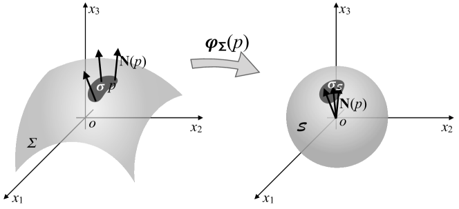
Figure 7.4: The map of Gauss.

We want to study how $\mathbf{N}(p)$ varies at the varying of $p$ on $\Sigma$. The idea is that the change of $\mathbf{N}(p)$ on $\Sigma$ is related to the curvature of the surface. For this purpose, we calculate the change in $\mathbf{N}$ per unit length of a curve $\boldsymbol{\gamma}(s)\in\Sigma$, i.e. we study how $\mathbf{N}$ varies along any curve of $\Sigma$ per unit of length of the curve itself; that is why we parameterize the curve with its arc-length $s$ . Let $\mathbf{N}=N_{i}(u,v)\mathbf{e}_{i}$; then, if $\boldsymbol{\tau}\in\mathcal{S}$ is the tangent to the curve,

$$\begin{split}\frac{d\mathbf{N}}{ds}&=\frac{dN_{i}(u(s),v(s))}{ds}\mathbf{e}_{i}=\left(\frac{\partial N_{i}}{\partial u}\frac{du}{ds}+\frac{\partial N_{i}}{\partial v}\frac{dv}{ds}\right)\mathbf{e}_{i}\\ &=\nabla N_{i}\cdot\boldsymbol{\tau}\mathbf{e}_{i}=(\mathbf{e}_{i}\otimes\nabla N_{i})\boldsymbol{\tau}=(\nabla\mathbf{N})\ \boldsymbol{\tau}=\frac{d\mathbf{N}}{d\boldsymbol{\tau}}.\end{split}$$

The change in $\mathbf{N}$ is hence related to the directional derivative of $\mathbf{N}$ along the tangent $\boldsymbol{\tau}$ to $\boldsymbol{\gamma}(s)$, which is a linear operator on $T_{p}\Sigma$. Moreover, as $\mathbf{N}\in\mathcal{S}$, then, cf. Eq. (4.1),

$$\mathbf{N}\cdot\mathbf{N}_{,u}=\mathbf{N}\cdot\mathbf{N}_{,v}=0\ \Rightarrow\ \mathbf{N}_{,u},\mathbf{N}_{,v}\in T_{p}\Sigma.$$

We then call Weingarten operator $\mathcal{L}_{W}:T_{p}\Sigma\rightarrow T_{p}\Sigma$ the opposite of the directional derivative of $\mathbf{N}$:

$$\mathcal{L}_{W}(\boldsymbol{\tau}):=-\frac{d\mathbf{N}}{d\boldsymbol{\tau}}.$$

Hence,

$$\mathcal{L}_{W}(\mathbf{f}_{,u})=-\mathbf{N}_{,u},\ \ \mathcal{L}_{W}(\mathbf{f}_{,v})=-\mathbf{N}_{,v}.$$ (7.10)

Because $\mathcal{L}_{W}$ is linear, then there exists a tensor $\mathbf{X}$ on $T_{p}\Sigma$ such that

$$\mathcal{L}_{W}(\mathbf{v})=\mathbf{X}\mathbf{v}\ \ \ \forall\mathbf{v}\in T_{p}\Sigma.$$ (7.11)

For any two vectors $\mathbf{w}_{1},\mathbf{w}_{2}\in T_{p}\Sigma$, we define second fundamental form of a surface, denoted by $II(\mathbf{w}_{1},\mathbf{w}_{2})$ the bilinear form

$$II(\mathbf{w}_{1},\mathbf{w}_{2}):=I(\mathcal{L}_{W}(\mathbf{w}_{1}),\mathbf{w}_{2}).$$

Theorem 43.

(Symmetry of the second fundamental form). $\forall\mathbf{w}_{1},\mathbf{w}_{2}\in T_{p}\Sigma,\ II(\mathbf{w}_{1},\mathbf{w}_{2})=II(\mathbf{w}_{2},\mathbf{w}_{1})$.

Proof.

Because $I$ and $\mathcal{L}_{W}$ are linear, it is sufficient to prove the thesis for the natural basis $\{\mathbf{f}_{,u},\mathbf{f}_{,v}\}$ of $T_{p}\Sigma$, and, by the symmetry of $I$, it is sufficient to prove that

$$I(\mathcal{L}_{W}(\mathbf{f}_{,u}),\mathbf{f}_{,v})=I(\mathbf{f}_{,u},\mathcal{L}_{W}(\mathbf{f}_{,v})),$$

i.e. that

$$I(-\mathbf{N}_{,u},\mathbf{f}_{,v})=I(\mathbf{f}_{,u},-\mathbf{N}_{,v})$$

and in the end that

$$\mathbf{N}_{,u}\cdot\mathbf{f}_{,v}=\mathbf{f}_{,u}\cdot\mathbf{N}_{,v}.$$

To this purpose, we recall that

$$\mathbf{N}\cdot\mathbf{f}_{,u}=0=\mathbf{N}\cdot\mathbf{f}_{,v}.$$

So, differentiating the first equation by $v$ and the second one by $u$, we get

$$\mathbf{N}_{,v}\cdot\mathbf{f}_{,u}=-\mathbf{N}\cdot\mathbf{f}_{,uv}=\mathbf{N}_{,u}\cdot\mathbf{f}_{,v}.$$ (7.12)

∎

The second fundamental form defines a quadratic, bilinear symmetric form:

$$\begin{split}II(\mathbf{w}_{1},\mathbf{w}_{2})&=I(\mathcal{L}_{W}(\mathbf{w}_{1}),\mathbf{w}_{2})=I(\mathbf{w}_{1},\mathcal{L}_{W}(\mathbf{w}_{2}))\\ &=I(\mathbf{w}_{1},\mathbf{X}\mathbf{w}_{2})=\mathbf{w}_{1}\cdot\mathbf{g}\mathbf{X}\mathbf{w}_{2}=\mathbf{w}_{1}\cdot\mathbf{B}\mathbf{w}_{2},\end{split}$$

where

$$\mathbf{B}:=\mathbf{g}\mathbf{X}.$$ (7.13)

In the natural basis $\{\mathbf{f}_{,u},\mathbf{f}_{,v}\}$ of $T_{p}\Sigma$, by Eq. (7.12), it is

$$B_{ij}=II(\mathbf{f}_{,i},\mathbf{f}_{,j})=I(\mathcal{L}_{W}(\mathbf{f}_{,i}),\mathbf{f}_{,j})=-\mathbf{N}_{,i}\cdot\mathbf{f}_{,j}=\mathbf{N}\cdot\mathbf{f}_{,ij};$$ (7.14)

tensor $\mathbf{X}$ can then be calculated by Eq. (7.13):

$$\mathbf{X}=\mathbf{g}^{-1}\mathbf{B}.$$ (7.15)

By Eq. (7.14), because $\mathbf{f}_{,ij}=\mathbf{f}_{,ji}$ or simply because $II(\cdot,\cdot)$ is symmetric, we get that

$$\mathbf{B}=\mathbf{B}^{\top}.$$

7.6 Curvatures of a surface

Let $\mathbf{f}:\Omega\rightarrow\Sigma$ be a regular surface and $\boldsymbol{\gamma}(s):G\subset\mathbb{R}\rightarrow\Sigma$ be a regular curve on $\Sigma$ parameterized with the arc length $s$. We call curvature vector of $\boldsymbol{\gamma}(s)$ the vector $\boldsymbol{\kappa}(s)$ defined as

$$\boldsymbol{\kappa}(s):=c(s)\boldsymbol{\nu}(s)=\boldsymbol{\gamma}^{\prime\prime}(s),$$

where $\boldsymbol{\nu}(s)$ is the principal normal to $\boldsymbol{\gamma}(s)$. By Eq. (4.11), it is also

$$\boldsymbol{\kappa}(s)=\boldsymbol{\gamma}^{\prime\prime}(s).$$

Then, we call normal curvature $\kappa_{N}(s)$ of $\boldsymbol{\gamma}(s)$ the projection of $\boldsymbol{\kappa}(s)$ onto $\mathbf{N}(s)$, the normal to $\Sigma$:

$$\kappa_{N}(s):=\boldsymbol{\kappa}(s)\cdot\mathbf{N}(s)=c(s)\ \boldsymbol{\nu}(s)\cdot\mathbf{N}(s)=\boldsymbol{\gamma}^{\prime\prime}(s)\cdot\mathbf{N}(s).$$

Theorem 44.

The normal curvature $\kappa_{N}(s)$ of $\boldsymbol{\gamma}(s)\in\Sigma$ depends uniquely on $\boldsymbol{\tau}(s)$:

$$\kappa_{N}(s)=\boldsymbol{\tau}(s)\cdot\mathbf{B}\boldsymbol{\tau}(s)=II(\boldsymbol{\tau}(s),\boldsymbol{\tau}(s)).$$ (7.16)

Proof.

$$\boldsymbol{\gamma}(s)=\boldsymbol{\gamma}(u(s),v(s))\ \rightarrow\ \boldsymbol{\tau}(s)=\boldsymbol{\gamma}^{\prime}(s)=\mathbf{f}_{,u}u^{\prime}+\mathbf{f}_{,v}v^{\prime},$$

therefore $\boldsymbol{\tau}=(u^{\prime},v^{\prime})$ in the natural basis and

$$\boldsymbol{\kappa}(s)=\boldsymbol{\gamma}^{\prime\prime}(s)=\mathbf{f}_{,u}u^{\prime\prime}+\mathbf{f}_{,v}v^{\prime\prime}+\mathbf{f}_{,uu}u^{\prime 2}+2\mathbf{f}_{,uv}u^{\prime}v^{\prime}+\mathbf{f}_{,vv}v^{\prime 2}$$

and finally, by Eqs. (7.2) and (7.14),

$$\kappa_{N}(s)=\boldsymbol{\gamma}^{\prime\prime}(s)\cdot\mathbf{N}(s)=B_{11}u^{\prime 2}+2B_{12}u^{\prime}v^{\prime}+B_{22}v^{\prime 2}=\boldsymbol{\tau}\cdot\mathbf{B}\boldsymbol{\tau}=II(\boldsymbol{\tau},\boldsymbol{\tau}).$$

∎

If now $s=s(t)$ is a change of parameter for $\boldsymbol{\gamma}$, then

$$\boldsymbol{\gamma}^{\prime}(t)=|\boldsymbol{\gamma}^{\prime}(t)|\boldsymbol{\tau}(t),$$

so by the linearity of $II(\cdot,\cdot)$, we get

$$II(\boldsymbol{\gamma}^{\prime}(t),\boldsymbol{\gamma}^{\prime}(t))=|\boldsymbol{\gamma}^{\prime}(t)|^{2}II(\boldsymbol{\tau}(t),\boldsymbol{\tau}(t))=|\boldsymbol{\gamma}^{\prime}(t)|^{2}\kappa_{N}(t)$$

and finally,

$$\kappa_{N}(t)=\frac{II(\boldsymbol{\gamma}^{\prime}(t),\boldsymbol{\gamma}^{\prime}(t))}{I(\boldsymbol{\gamma}^{\prime}(t),\boldsymbol{\gamma}^{\prime}(t))}.$$

To each point $p\in\Sigma$, it corresponds uniquely (in the assumption of regularity of the surface $\mathbf{f}:\Omega\rightarrow\Sigma$) a tangent plane and a tangent space vector $T_{p}\Sigma$. In $p$, there are infinite tangent vectors to $\Sigma$, all of them belonging to $T_{p}\Sigma$. We can associate a curvature to each direction $\mathbf{t}\in T_{p}\Sigma$, i.e. to each tangent direction, in the following way: Let us consider the bundle $\mathcal{H}$ of planes whose support is the straight line through $p$ and parallel to $\mathbf{N}$. Then, any plane $H\in\mathcal{H}$ is a normal plane to $\Sigma$ in $p$; each normal plane is uniquely determined by a tangent direction $\mathbf{t}$ and the (planar) curve $\boldsymbol{\gamma}_{N\mathbf{t}}:=H\cap\Sigma$ is called a normal section of $\Sigma$. If $\boldsymbol{\nu}$ and $\mathbf{N}$ are, respectively, the principal normal to $\boldsymbol{\gamma}_{N\mathbf{t}}$ and the normal to $\Sigma$ in $p$, then

$$\boldsymbol{\nu}=\pm\mathbf{N}$$

for each normal section. We have, in this way, defined a function that to each tangent direction $\mathbf{t}\in T_{p}\Sigma$ associates the normal curvature $\kappa_{N}$ of the normal section $\boldsymbol{\gamma}_{N\mathbf{t}}$:

$$\kappa_{N}:\mathcal{S}\cap T_{p}\Sigma\rightarrow\mathbb{R}|\ \ \ \kappa_{N}(\mathbf{t})=\frac{II(\mathbf{t},\mathbf{t})}{I(\mathbf{t},\mathbf{t})}.$$

By the bilinearity of the second fundamental form, $\kappa_{N}(\mathbf{t})=\kappa_{N}(-\mathbf{t})$.

A point $p\in\Sigma$ is said to be a umbilical point if $\kappa_{N}(\mathbf{t})=const.\ \forall\mathbf{t}$, it is a planar point if $\kappa_{N}(\mathbf{t})=0\ \forall\mathbf{t}$. In all the other points, $\kappa_{N}$ takes a minimum and a maximum value on distinct directions $\mathbf{t}\in T_{p}\Sigma$.

Because $\mathbf{B}=\mathbf{B}^{\top}$, by the spectral theorem, there exists an orthonormal basis $\{\mathbf{u}_{1},\mathbf{u}_{2}\}$ of $T_{p}\Sigma$ such that

$$\mathbf{B}=\beta_{j}\mathbf{u}_{j}\otimes\mathbf{u}_{j},$$

with $\beta_{j}$ the eigenvalues of $\mathbf{B}$. In such a basis, by Eq. (7.13) we get

$$\kappa_{N}(\mathbf{u}_{i})=\frac{II(\mathbf{u}_{\underline{i}},\mathbf{u}_{\underline{i}})}{I(\mathbf{u}_{\underline{i}},\mathbf{u}_{\underline{i}})}=\frac{\mathbf{u}_{\underline{i}}\cdot\mathbf{B}\mathbf{u}_{\underline{i}}}{\mathbf{u}_{\underline{i}}\cdot\mathbf{g}\mathbf{u}_{\underline{i}}}=\frac{\mathbf{u}_{\underline{i}}\cdot\mathbf{g}\mathbf{X}\mathbf{u}_{\underline{i}}}{\mathbf{u}_{\underline{i}}\cdot\mathbf{g}\mathbf{u}_{\underline{i}}},\ \ \ i=1,2.$$

Then, because $\{\mathbf{u}_{1},\mathbf{u}_{2}\}$ is an orthonormal basis, $\mathbf{g}=\mathbf{I}$ and

$$\kappa_{N}(\mathbf{u}_{i})=\mathbf{u}_{\underline{i}}\cdot\mathbf{X}\mathbf{u}_{\underline{i}},\ \ \ i=1,2,$$

i.e. $\mathbf{X}$ and $\mathbf{B}$ share the same eigenvectors. Moreover, cf. Section 2.8, we know that the two directions $\mathbf{u}_{1}$ and $\mathbf{u}_{2}$ are the directions whereupon the quadratic form in the previous equation gets its maximum, $\kappa_{1}$, and minimum, $\kappa_{2}$, values, and in such a basis,

$$\mathbf{X}=\kappa_{i}\mathbf{u}_{i}\otimes\mathbf{u}_{i}.$$

We call $\kappa_{1}$ and $\kappa_{2}$ the principal curvatures of $\Sigma$ in $p$ and $\mathbf{u}_{1},\mathbf{u}_{2}$ the principal directions of $\Sigma$ in $p$, see Fig. 7.5.

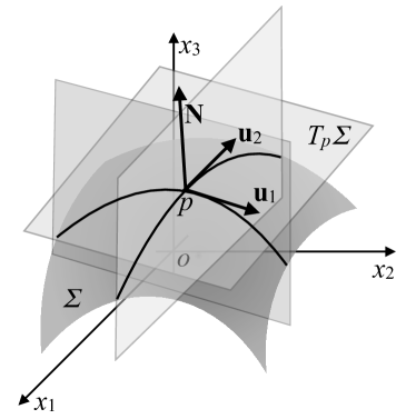
Figure 7.5: Principal curvatures.

We call Gaussian curvature $K$ the product of the principal curvatures:

$$K:=\kappa_{1}\kappa_{2}=\det\mathbf{X}.$$

By Eq. (7.15) and the theorem of Binet, it is also

$$K=\frac{\det\mathbf{B}}{\det\mathbf{g}}.$$ (7.17)

We define mean curvature $H$ of a surface $\mathbf{f}:\Omega\rightarrow\Sigma$ at a point $p\in\Sigma$ the mean of the principal curvatures at $p$:

$$H:=\frac{\kappa_{1}+\kappa_{2}}{2}=\frac{1}{2}\mathrm{tr}\mathbf{X}.$$

Of course, a change in the parameterization of a surface can change the orientation, cf. Section 7.1, i.e. it can transforms $\mathbf{N}$ into its opposite one and, by consequence, change the sign of the second fundamental form and hence of the normal and principal curvatures. These last are hence defined to less the sign, and the mean curvature too, while the principal directions, umbilicality, flatness and Gaussian curvature are intrinsic to $\Sigma$, i.e. they do not depend on its parameterization.

7.7 The theorem of Rodrigues

Then principal directions of curvature have a property which is specified by the

Theorem 45.

(Theoreom of Rodrigues). Let $\mathbf{f}(u,v)$ be a surface of class at least C² and $\boldsymbol{\lambda}=(\lambda_{u},\lambda_{v})\in T_{p}\Sigma$; then

$$\frac{d\mathbf{N}(p)}{d\boldsymbol{\lambda}}=-\kappa_{\lambda}\boldsymbol{\lambda}$$ (7.18)

if and only if $\boldsymbol{\lambda}$ is a principal direction; $\kappa_{\lambda}$ is the principal curvature relative to $\boldsymbol{\lambda}$.

Proof.

Let $\boldsymbol{\lambda}$ be a principal direction of $T_{p}\Sigma$. Because $\mathbf{N}\in\mathcal{S}$, then

$$\frac{d\mathbf{N}}{d\boldsymbol{\lambda}}\cdot\mathbf{N}=0;$$ (7.19)

moreover,

$$\frac{d\mathbf{N}}{d\boldsymbol{\lambda}}=\nabla\mathbf{N}\ \boldsymbol{\lambda}=\left[\begin{array}[]{ccc}0&0&0\\ 0&0&0\\ \mathbf{N}_{,u}&\mathbf{N}_{,v}&1\end{array}\right]\left\{\begin{array}[]{c}\lambda_{u}\\ \lambda_{v}\\ 0\end{array}\right\}=\mathbf{N}_{,u}\lambda_{u}+\mathbf{N}_{,v}\lambda_{v}.$$ (7.20)

Let $\boldsymbol{\mu}=(\mu_{u},\mu_{v})$ be the other principal direction of $T_{p}\Sigma$, then

$$\boldsymbol{\lambda}\cdot\boldsymbol{\mu}=0\ \rightarrow\ I(\boldsymbol{\lambda},\boldsymbol{\mu})=II(\boldsymbol{\lambda},\boldsymbol{\mu})=0.$$

Moreover,

$$\frac{d\mathbf{N}}{d\boldsymbol{\lambda}}\cdot\boldsymbol{\mu}=-II(\boldsymbol{\lambda},\boldsymbol{\mu})=0,$$

which implies, together with Eq. (7.19),

$$\frac{d\mathbf{N}}{d\boldsymbol{\lambda}}=\alpha\boldsymbol{\lambda}.$$ (7.21)

Therefore,

$$\frac{d\mathbf{N}}{d\boldsymbol{\lambda}}\cdot\boldsymbol{\lambda}=-II(\boldsymbol{\lambda})=\alpha\boldsymbol{\lambda}\cdot\boldsymbol{\lambda}=\alpha I(\boldsymbol{\lambda})$$

and finally,

$$\alpha=-\frac{II(\boldsymbol{\lambda})}{I(\boldsymbol{\lambda})}=-\kappa_{\lambda}.$$

Contrarily, if we assume Eq. (7.21), as before we get $\alpha=-\kappa_{\lambda}$ and to end, we just need to prove that $\boldsymbol{\lambda}$ is a principal direction. From Eqs. (7.20) and (7.21), we get

$$\lambda_{u}\mathbf{N}_{,u}+\lambda_{v}\mathbf{N}_{,v}=-\kappa_{\lambda}(\lambda_{u}\mathbf{f}_{,u}+\lambda_{v}\mathbf{f}_{,v}).$$

Projecting this equation onto $\mathbf{f}_{,u}$ and $\mathbf{f}_{,v}$ gives the two equations

$$\begin{split}&L\lambda_{u}+M\lambda_{v}=\kappa_{\lambda}(E\lambda_{u}+F\lambda_{v}),\\ &M\lambda_{u}+N\lambda_{v}=\kappa_{\lambda}(E\lambda_{u}+G\lambda_{v}),\end{split}$$ (7.22)

with the symbols $E,F,G,L,M$ and $N$ defined in Notes 3 and 7 and used here for the sake of conciseness. Let $\mathbf{w}=(w_{u},w_{v})\in T_{p}\Sigma$ and consider the function

$$\zeta(\mathbf{w},\kappa_{\lambda})=II(\mathbf{w})-\kappa_{\lambda}I(\mathbf{w});$$

it is easy to check that $\zeta,\dfrac{\partial\zeta}{\partial w_{u}}$ and $\dfrac{\partial\zeta}{\partial w_{v}}$ take zero value for $\mathbf{w}=\boldsymbol{\lambda}_{0}$, with $\boldsymbol{\lambda}_{0}$ the eigenvector of the principal direction relative to $\kappa_{\lambda}$, which gives the system of equations

$$\left\{\begin{split}&II(\boldsymbol{\lambda}_{0})-\kappa_{\lambda}I(\boldsymbol{\lambda}_{0})=0,\\ &\frac{\partial II(\boldsymbol{\lambda}_{0})}{\partial w_{u}}-\kappa_{\lambda}\frac{\partial II(\boldsymbol{\lambda}_{0})}{\partial w_{u}}=0,\\ &\frac{\partial II(\boldsymbol{\lambda}_{0})}{\partial w_{v}}-\kappa_{\lambda}\frac{\partial II(\boldsymbol{\lambda}_{0})}{\partial w_{v}}=0.\end{split}\right.$$

Developing the derivatives and making some standard passages, Eq. (7.22) is found again, which proves that $\boldsymbol{\lambda}$ is necessarily the principal direction relative to $\kappa_{\lambda}$. ∎

This theorems hence states that the derivative of $\mathbf{N}$ along a given direction is a vector parallel to such a direction only when this is a principal direction of curvature.

7.8 Classification of the points of a surface

Let $\mathbf{f}:\Omega\rightarrow\Sigma$ be a regular surface and $p\in\Sigma$ a non-planar point. Then, we say that

• $p$ is an elliptic point if $K(p)>0$;

• $p$ is a hyperbolic point if $K(p)<0$;

• $p$ is a parabolic point if $K(p)=0$.

We remark that, by Eq. (7.17), because $\det\mathbf{g}>0$, Eq. (6.4), the value of $\det\mathbf{B}$ is sufficient to determine the type of a point on $\Sigma$.

Theorem 46.

If $p$ is an elliptical point of $\sigma$, then there exists a neighbourhood $U\in\Sigma$ of $p$ such that all the points $q\in U$ belong to the same half-space into which $\mathcal{E}$ is divided by the tangent plane $T_{p}\Sigma$.

Proof.

For the sake of simplicity and without loss of generality, we can always chose a parameterization $\mathbf{f}(u,v)$ of the surface such that $p=\mathbf{f}(0,0)$. Expanding $\mathbf{f}(u,v)$ into a Taylor’s series around $(0,0)$, we get the position of a point $q=\mathbf{f}(u,v)\in\Sigma$ in the nighbourhood of $p$ (though not indicated for the sake of brevity, all the derivatives are intended to be calculated at $(0,0)$):

$$\mathbf{f}(u,v)=\mathbf{f}_{,u}u+\mathbf{f}_{,v}v+\frac{1}{2}(\mathbf{f}_{,uu}u^{2}+2\mathbf{f}_{,uv}uv+\mathbf{f}_{,vv}v^{2})+o(u^{2}+v^{2}).$$

The distance with sign $d(q)$ of $q\in\Sigma$ from the tangent plane $T_{p}\Sigma$ is the projection onto $\mathbf{N}$, i.e.:

$$\begin{split}d(q)&=\frac{1}{2}(\mathbf{f}_{,uu}u^{2}+2\mathbf{f}_{,uv}uv+\mathbf{f}_{,vv}v^{2})\cdot\mathbf{N}+o(u^{2}+v^{2})\\ &=\frac{1}{2}(B_{11}u^{2}+2B_{12}uv+B_{22}v^{2})+o(u^{2}+v^{2}),\end{split}$$

or, equivalently, once we set $\mathbf{w}=u\mathbf{f}_{,u}+v\mathbf{f}_{,v}$,

$$d(q)=\frac{1}{2}II(\mathbf{w},\mathbf{w})+o(u^{2}+v^{2}).$$ (7.23)

If $p$ is an elliptic point, the principal curvatures have the same sign because $K=\kappa_{1}\kappa_{2}>0\Rightarrow$ the sign of $II(\mathbf{w},\mathbf{w})$ does not depend upon $\mathbf{w}$, i.e. upon the tangent vector. As a consequence the sign of $d(q)$ does not change with $\mathbf{w}\Rightarrow\forall q\in U,\ \Sigma$ is on the same side of the tangent plane $T_{p}\Sigma$. ∎

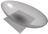
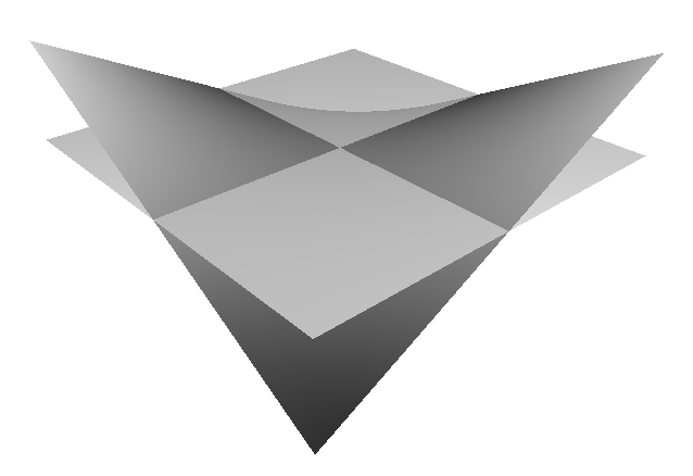
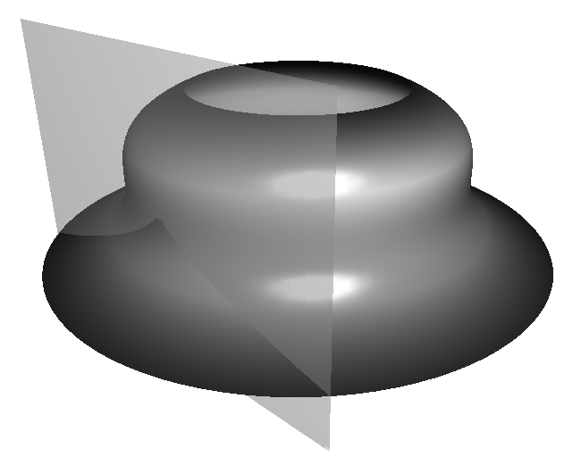
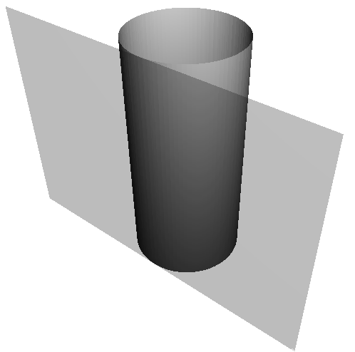
Figure 7.6: Elliptic (left), hyperbolic (center), and parabolic (last two on the right), points.

Theorem 47.

If $p$ is a hyperbolic point of $\Sigma$, then for each neighbourhood $U\in\Sigma$ of $p$, there are points $q\in U$ that are in half-spaces on the opposite sides with respect to the tangent plane $T_{p}\Sigma$.

Proof.

The proof is identical to that of the previous theorem until Eq. (7.23); now, if $p$ is a hyperbolic point, the principal curvatures have opposite signs and by consequence $d(q)$ changes of sign at least two times in any neighbourhood $U$ of $p\Rightarrow$ there are points $q\in U$ lying in half-spaces on the opposite sides with respect to the tangent plane $T_{p}\Sigma$. ∎

In a parabolic point, there are different possibilities: $\Sigma$ is on one side of the space with respect to $T_{p}\Sigma$, like for the case of a cylinder, or not, like, as an example, for the points $(0,v)$ of the surface, see Fig. 7.6,

$$\left\{\begin{array}[]{l}x=(u^{3}+2)\cos v,\\ y=(u^{3}+2)\sin v,\\ z=-u.\end{array}\right.$$

This is also the case for planar points: e.g., the point $(0,0,0)$ is a planar point for both the surfaces

$$z=x^{4}+y^{4},\ \ \ z=x^{3}-3xy^{2},$$

but in the first case, all the surface is on one side of the tangent plane, while it is on both sides for the second case (the so-called monkey’s saddle), see Fig.7.7.

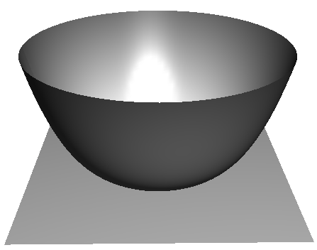
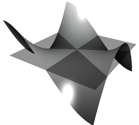
Figure 7.7: Two different planar points.

7.9 Developable surfaces

Let us now consider a ruled surface $\mathbf{f}:\Omega\rightarrow\Sigma$ as in Eq. (7.7); then

$$\mathbf{f}_{,u}=\boldsymbol{\gamma}^{\prime}+v\boldsymbol{\lambda}^{\prime},\ \ \mathbf{f}_{,v}=\boldsymbol{\lambda},\ \ \mathbf{f}_{,u}\times\mathbf{f}_{,v}=\boldsymbol{\gamma}^{\prime}\times\boldsymbol{\lambda}+v\boldsymbol{\lambda}^{\prime}\times\boldsymbol{\lambda},\ \ \mathbf{f}_{,uv}=\boldsymbol{\lambda}^{\prime},\ \ \mathbf{f}_{,vv}=\mathbf{o}.$$

Consequently, $B_{22}=\mathbf{N}\cdot\mathbf{f}_{,vv}=0\ \Rightarrow\ \det\mathbf{B}=-B_{12}^{2}$: The points of $\Sigma$ are hyperbolic or parabolic. Namely, the parabolic points are those with

$$B_{12}=\mathbf{N}\cdot\mathbf{f}_{,uv}=\frac{\mathbf{f}_{,u}\times\mathbf{f}_{,v}}{|\mathbf{f}_{,u}\times\mathbf{f}_{,v}|}\cdot\mathbf{f}_{,uv}=0\ \iff\ (\boldsymbol{\gamma}^{\prime}\times\boldsymbol{\lambda}+v\boldsymbol{\lambda}^{\prime}\times\boldsymbol{\lambda})\cdot\boldsymbol{\lambda}^{\prime}=\boldsymbol{\gamma}^{\prime}\times\boldsymbol{\lambda}\cdot\boldsymbol{\lambda}^{\prime}=0.$$

We remark that the ruled surfaces made of parabolic points have null Gaussian curvature everywhere: $K=0$.

Let us consider ruled surfaces having only parabolic points; then, we have the following

Theorem 48.

For a ruled surface $\mathbf{f}(u,v)=\boldsymbol{\gamma}(u)+v\boldsymbol{\lambda}(u)$, the following are equivalents:

1. $\boldsymbol{\gamma}^{\prime},\boldsymbol{\lambda},\boldsymbol{\lambda}^{\prime}$ are linearly dependent;

2. $\mathbf{N}_{,v}=\mathbf{o}$.

Proof.

Condition $ii$ implies that $\mathbf{N}$ does not change along a straight line lying on the ruled surface $\Rightarrow\mathbf{f}_{,u}\times\mathbf{f}_{,v}=\boldsymbol{\gamma}^{\prime}\times\boldsymbol{\lambda}+v\boldsymbol{\lambda}^{\prime}\times\boldsymbol{\lambda}$ does not depend on $v$ as well. This is possible $\iff\boldsymbol{\gamma}^{\prime}\times\boldsymbol{\lambda}$ and $\boldsymbol{\lambda}^{\prime}\times\boldsymbol{\lambda}$ are linearly dependent, i.e. $\iff$

$$(\boldsymbol{\gamma}^{\prime}\times\boldsymbol{\lambda})\times(\boldsymbol{\lambda}^{\prime}\times\boldsymbol{\lambda})=(\boldsymbol{\lambda}^{\prime}\times\boldsymbol{\lambda}\cdot\boldsymbol{\gamma}^{\prime})\boldsymbol{\lambda}-(\boldsymbol{\lambda}^{\prime}\times\boldsymbol{\lambda}\cdot\boldsymbol{\lambda})\boldsymbol{\gamma}^{\prime}=(\boldsymbol{\lambda}^{\prime}\times\boldsymbol{\lambda}\cdot\boldsymbol{\gamma}^{\prime})\boldsymbol{\lambda}=\mathbf{o},$$

i.e. when $\boldsymbol{\lambda},\boldsymbol{\lambda}^{\prime}$ and $\boldsymbol{\gamma}^{\prime}$ are coplanar, which proves the thesis. ∎

We say that a ruled surface is developable if one of the conditions of Theorem 48 is satisfied. A developable surface is a surface that can be flattened without distortion onto a plane, i.e. it can be bent without stretching or shearing or, vice-versa, it can be obtained by transforming a plane. We remark that only ruled surfaces are developable (but not all the ruled surfaces are developable).

It is immediate to check that a cylinder or a cone are developable surfaces, while the helicoid, the hyperbolic hyperboloid or the hyperbolic paraboloid are not. Another classical example of developable surface is the ruled surface of the tangents to a curve: Let $\boldsymbol{\gamma}(t):G\subset\mathbb{R}\rightarrow\mathcal{E}$ be a regular smooth curve; then the ruled surface of the tangents to $\boldsymbol{\gamma}$ is the surface $\mathbf{f}(u,v):G\times\mathbb{R}\rightarrow\Sigma$ defined by

$$\mathbf{f}(u,v)=\boldsymbol{\gamma}(u)+v\boldsymbol{\gamma}^{\prime}(u).$$

Fig. 7.8 shows the ruled surface of the tangents to a cylindrical helix.

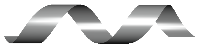
Figure 7.8: The ruled surface of the tangents to a cylindrical helix.

7.10 Points of a surface of revolution

Let us now consider a surface of revolution $\mathbf{f}:\Omega\rightarrow\Sigma_{\gamma}$ as in Eq. (7.5) and, for the sake of simplicity, let $u$ be the natural parameter of the curve $\boldsymbol{\gamma}(u)$ in Eq. (7.4) generating the surface. Then

$$\varphi^{\prime 2}(u)+\psi^{\prime 2}(u)=1,\ \ \ \ \psi^{\prime\prime}(u)\varphi^{\prime}(u)-\psi^{\prime}(u)\varphi^{\prime\prime}(u)=c(u).$$

We can then calculate:

• the vectors of the natural basis:

  $$\mathbf{f}_{,u}=\left\{\begin{array}[]{c}\varphi^{\prime}(u)\cos v\\ \varphi^{\prime}(u)\sin v\\ \psi^{\prime}(u)\end{array}\right\},\ \ \ \ \ \mathbf{f}_{,v}=\left\{\begin{array}[]{c}-\varphi(u)\sin v\\ \varphi(u)\cos v\\ 0\end{array}\right\};$$

• the normal to the surface

  $$\mathbf{N}=\left\{\begin{array}[]{c}-\psi^{\prime}(u)\cos v\\ -\psi^{\prime}(u)\sin v\\ \varphi^{\prime}(u)\end{array}\right\};$$

• the metric tensor (i.e. the first fundamental form):

  $$\mathbf{g}=\left[\begin{array}[]{cc}1&0\\ 0&\varphi^{2}(u)\end{array}\right];$$

• the second derivatives of $\mathbf{f}$:

  $$\mathbf{f}_{,uu}=\left\{\begin{array}[]{c}\varphi^{\prime\prime}(u)\cos v\\ \varphi^{\prime\prime}(u)\sin v\\ \psi^{\prime\prime}(u)\end{array}\right\},\ \ \ \mathbf{f}_{,uv}=\left\{\begin{array}[]{c}-\varphi^{\prime}(u)\sin v\\ \varphi^{\prime}(u)\cos v\\ 0\end{array}\right\},\ \ \ \mathbf{f}_{,vv}=\left\{\begin{array}[]{c}-\varphi(u)\cos v\\ -\varphi(u)\sin v\\ 0\end{array}\right\};$$

• tensor $\mathbf{B}$ (i.e. the second fundamental form):

  $$\mathbf{B}=\left[\begin{array}[]{cc}c(u)&0\\ 0&\varphi(u)\psi^{\prime}(u)\end{array}\right];$$

• the Gaussian curvature $K$:

  $$K=\det\mathbf{X}=\frac{\det\mathbf{B}}{\det\mathbf{g}}=\frac{c(u)\psi^{\prime}(u)}{\varphi(u)}.$$

Therefore, points of $\Sigma_{\gamma}$ where $c(u)$ and $\psi^{\prime}(u)$ have the same sign are elliptic, but hyperbolic otherwise. Parabolic points correspond to inflexion points of $\boldsymbol{\gamma}(u)$ if $c(u)=0$, or to points with horizontal tangent to $\boldsymbol{\gamma}(u)$ if $\psi^{\prime}(u)=0$.

As an example, let us consider the case of the pseudo-sphere, Eq. (7.6). Then,

$$\varphi(u)=\sin u,\ \ \ \psi(u)=\cos u+\ln\tan\frac{u}{2}.$$

Some simple calculations give ($u$ is not the arc-length of $\boldsymbol{\gamma}(u)$, which actually is a tractrix, see Exercise 9, Chapter 4; hence $|\boldsymbol{\gamma}^{\prime}(u)|=\sqrt{\varphi^{\prime 2}(u)+\psi^{\prime 2}(u)}\neq 1$)

$$\psi^{\prime}(u)=-\sin u+\frac{1}{\sin u},\ \ \ c(u)=-|\tan u|;$$

as a consequence

$$K=\frac{c(u)\psi^{\prime}(u)}{\varphi(u)\sqrt{\varphi^{\prime 2}(u)+\psi^{\prime 2}(u)}}=-\frac{(-\sin u+\frac{1}{\sin u})|\tan u|}{\sin u|\cot u|}=-1.$$

Finally, $K=const.=-1$, which is the reason for the name of this surface.

7.11 Lines of curvature, conjugated directions, asymptotic directions

A line of curvature is a curve on a surface with the property of being tangent, at each point, to a principal direction.

Theorem 49.

The lines of curvature of a surface are the solutions to the differential equation

$$X_{21}u^{\prime 2}+(X_{22}-X_{11})u^{\prime}v^{\prime}-X_{12}v^{\prime 2}=0.$$

Proof.

A curve $\boldsymbol{\gamma}(t):G\subset\mathbb{R}\rightarrow\Sigma\subset\mathcal{E}$ is a line of curvature $\iff$

$$\boldsymbol{\gamma}^{\prime}(t)=\mathbf{f}_{,u}u^{\prime}+\mathbf{f}_{,v}v^{\prime}$$

is an eigenvector of $\mathbf{X}(t)\ \forall t$, i.e. $\iff$ there exists a function $\mu(t)$ such that

$$\mathbf{X}(t)\boldsymbol{\gamma}^{\prime}(t)=\mu(t)\boldsymbol{\gamma}^{\prime}(t)\ \ \forall t.$$

In the natural basis of $T_{p}\Sigma$, this condition reads as (we omit the dependence upon $t$ for the sake of conciseness)

$$\left[\begin{array}[]{cc}X_{11}&X_{12}\\ X_{21}&X_{22}\end{array}\right]\left\{\begin{array}[]{c}u^{\prime}\\ v^{\prime}\end{array}\right\}=\mu\left\{\begin{array}[]{c}u^{\prime}\\ v^{\prime}\end{array}\right\},$$

which is satisfied $\iff$ the two vectors at the left- and right-hand sides are proportional, i.e. $\iff$

$$\det\left[\begin{array}[]{cc}X_{11}u^{\prime}+X_{12}v^{\prime}&u^{\prime}\\ X_{21}u^{\prime}+X_{22}v^{\prime}&v^{\prime}\end{array}\right]=0\ \rightarrow\ X_{21}u^{\prime 2}+(X_{22}-X_{11})u^{\prime}v^{\prime}-X_{12}v^{\prime 2}=0.$$

∎

As a corollary, if $\mathbf{X}$ is diagonal, then the coordinate lines are at the same time, principal directions and lines of curvature.

Theorem 50.

A curve $\boldsymbol{\gamma}(u):G\subset\mathbb{R}\rightarrow\Sigma$ is a line of curvature $\iff$ the surface

$$\mathbf{f}(u,v)=\boldsymbol{\gamma}(u)+v\mathbf{N}(\boldsymbol{\gamma}(u)),$$ (7.24)

is developable.

Proof.

From Theorem 48, $\mathbf{f}(u,v)$ is developable $\iff\boldsymbol{\gamma}^{\prime}\cdot\mathbf{N}\times\mathbf{N}^{\prime}=0$. Because $\boldsymbol{\gamma}^{\prime}$ and $\mathbf{N}^{\prime}\in T_{p}\Sigma$, which is orthogonal to $\mathbf{N}$, the surface will be developable $\iff\ \boldsymbol{\gamma}^{\prime}\times\mathbf{N}^{\prime}=\mathbf{o}$. Moreover, writing

$$\boldsymbol{\gamma}^{\prime}=\mathbf{f}_{,u}u^{\prime}+\mathbf{f}_{,v}v^{\prime}$$

it is

$$\mathbf{N}^{\prime}=\mathbf{N}_{,u}u^{\prime}+\mathbf{N}_{,v}v^{\prime}=-\mathcal{L}_{W}(\boldsymbol{\gamma}^{\prime}),$$

hence $\mathbf{f}(u,v)$ is developable $\iff\ \mathcal{L}_{W}(\boldsymbol{\gamma}^{\prime})\times\boldsymbol{\gamma}^{\prime}=\mathbf{o}$, i.e. when $\boldsymbol{\gamma}^{\prime}$ is a principal direction. ∎

The curve in Eq. (7.24) is called the ruled surface of the normals.

Let $p$ be a non-planar point of a surface $\mathbf{f}:\Omega\rightarrow\Sigma$ and $\mathbf{v}_{1},\mathbf{v}_{2}$ two vectors of $T_{p}\Sigma$. We say that $\mathbf{v}_{1}$ and $\mathbf{v}_{2}$ are conjugated if $II(\mathbf{v}_{1},\mathbf{v}_{2})=0$. The directions corresponding to $\mathbf{v}_{1}$ and $\mathbf{v}_{2}$ are called conjugated directions. Hence, the principal directions at a point $p$ are conjugated; if $p$ is an umbilical point, any two orthogonal directions are conjugated.

The direction of a vector $\mathbf{v}\in T_{p}\Sigma$ is said to be asymptotic if it is autoconjugated, i.e. if $II(\mathbf{v},\mathbf{v})=0$. An asymptotic direction is hence a direction where the normal curvature is null. In a hyperbolic point, there are two asymptotic directions, in a parabolic point only one and in an elliptic point, there are not asymptotic directions. An asymptotic line is a curve on a surface with the property of being tangent at every point to an asymptotic direction. The asymptotic lines are the solution of the differential equation

$$II(\boldsymbol{\gamma}^{\prime},\boldsymbol{\gamma}^{\prime})=0\ \rightarrow\ B_{11}u^{\prime 2}+2B_{12}u^{\prime}v^{\prime}+B_{22}v^{\prime 2}=0;$$

in particular, if $B_{11}=B_{22}=0$ and $\mathbf{B}\neq\mathbf{O}$, then the coordinate lines are asymptotic lines. Asymptotic lines exist only in the regions where $K\leq 0$.

7.12 The Dupin’s conical curves

The conical curves of Dupin are the real curves in $T_{p}\Sigma$ whose equations are

$$II(\mathbf{v},\mathbf{v})=\pm 1,\ \ \ \mathbf{v}\in\mathcal{S}.$$

Let $\{\mathbf{u}_{1},\mathbf{u}_{2}\}$ be the basis of the principal directions. Using polar coordinates, we can write

$$\mathbf{v}=\rho\mathbf{e}_{\rho},\ \ \ \mathbf{e}_{\rho}=\cos\theta\mathbf{u}_{1}+\sin\theta\mathbf{u}_{2}.$$

Therefore,

$$II(\mathbf{v},\mathbf{v})=\rho^{2}II(\mathbf{e}_{\rho},\mathbf{e}_{\rho})=\rho^{2}\kappa_{N}(\mathbf{e}_{\rho}),$$

and the conicals’ equations are

$$\rho^{2}(\kappa_{1}\cos^{2}\theta+\kappa_{2}\sin^{2}\theta)=\pm 1.$$

With the Cartesian coordinates $\xi=\rho\cos\theta,\eta=\rho\sin\theta$, we get

$$\kappa_{1}\xi^{2}+\kappa_{2}\eta^{2}=\pm 1.$$

The type of conical curves depend upon the kind of point on $\Sigma$:

• Elliptical points: The principal curvatures have the same sign $\rightarrow$ one of the conical curves is an ellipse, the other one the null set (actually, it is not a real curve).

• Hyperbolic points: The principal curvatures have opposite signs $\rightarrow$ the conical curves are conjugated hyperbolae whose asymptotes coincide with the asymptotic directions.

• Parabolic points: At least one of the principal curvatures is null $\rightarrow$ one of the conical curves degenerates into a couple of parallel straight lines, corresponding to the asymptotic direction, the other one is the null set.

The three possible cases are depicted in Fig. 7.9

Figure 7.9: The conical curves of Dupin; from the left: elliptic, hyperbolic and parabolic points.

7.13 The Gauss-Weingarten equations

Let $\mathbf{f}:\Omega\rightarrow\Sigma$ be a surface; for any point $p\in\Sigma$, consider the basis $\{\mathbf{f}_{,u},\mathbf{f}_{,v},\mathbf{N}\}$, also called the Gauss’ basis. It is the equivalent of the Frenet-Serret basis for the surfaces. We want to calculate the derivatives of the vectors of this basis, i.e. we want to obtain, for the surfaces, something equivalent to the Frenet-Serret equations.

$\mathbf{N}\in\mathcal{S}$ and $\mathbf{N}\cdot\mathbf{f}_{,u}=\mathbf{N}\cdot\mathbf{f}_{,v}=0$, but, in general, $\mathbf{f}_{,u},\mathbf{f}_{,v}\notin\mathcal{S}$ and $\mathbf{f}_{,u}\cdot\mathbf{f}_{,v}\neq 0$. In other words, we are dealing with a case of non-orthogonal (curvilinear) coordinates. So, if $w$ is the coordinate along the normal $\mathbf{N}$, let us call, for the sake of convenience,

$$u=z^{1},\ v=z^{2},$$

while, for the vectors,

$$\mathbf{f}_{,u}=\mathbf{f}_{,1}=\mathbf{g}_{1},\ \mathbf{f}_{,v}=\mathbf{f}_{,2}=\mathbf{g}_{2},$$

with $\mathbf{g}_{1},\mathbf{g}_{2}$ exactly the $\mathbf{g}$-vectors of the coordinate lines on $\Sigma$. Then (no summation on $i$ in the following equations),

$$\begin{split}&\frac{\partial\mathbf{g}_{i}}{\partial z^{j}}\cdot\mathbf{g}_{i}=\frac{1}{2}\frac{\partial(\mathbf{g}_{i}\cdot\mathbf{g}_{i})}{\partial z^{j}}=\frac{1}{2}\frac{\partial g_{ii}}{\partial z^{j}},\\ &\frac{\partial\mathbf{g}_{i}}{\partial z^{i}}\cdot\mathbf{g}_{j}=\frac{\partial(\mathbf{g}_{i}\cdot\mathbf{g}_{j})}{\partial z^{i}}-\frac{\partial\mathbf{g}_{i}}{\partial z^{j}}\cdot\mathbf{g}_{i}=\frac{\partial g_{ij}}{\partial z^{i}}-\frac{1}{2}\frac{\partial g_{ii}}{\partial z^{j}};\end{split}\ \ \ \ i,j=1,2;$$

for the last equation we have used the identity

$$\frac{\partial\mathbf{g}_{j}}{\partial z^{i}}=\mathbf{f}_{,ji}=\mathbf{f}_{,ij}=\frac{\partial\mathbf{g}_{i}}{\partial z^{j}},\ \ \ \ i,j=1,2.$$

Using Eq. (6.26), it can be proved that it is also

$$\frac{\partial\mathbf{g}_{i}}{\partial z^{j}}\cdot\mathbf{g}_{h}=\Gamma^{h}_{ij}\ \ \ \ i,j,h=1,2.$$

Moreover, by Eq. (7.14),

$$\frac{\partial\mathbf{g}_{i}}{\partial z^{j}}\cdot\mathbf{N}=\mathbf{f}_{,ij}\cdot\mathbf{N}=B_{ij}\ \ \ \ i,j=1,2,$$

and by Eqs. (7.10), (7.11),

$$\frac{\partial\mathbf{N}}{\partial z^{i}}\cdot\mathbf{g}_{j}=-\mathcal{L}_{W}(\mathbf{g}_{i})\cdot\mathbf{g}_{j}=-\mathbf{X}\mathbf{g}_{i}\cdot\mathbf{g}_{j}=-X_{ji},\ \ \ i,j=1,2,$$

while, because $\mathbf{N}\in\mathcal{S}$, then from Eq. (4.1),

$$\frac{\partial\mathbf{N}}{\partial z^{i}}\cdot\mathbf{N}=0\ \ \ \forall i=1,2.$$

Finally, the decomposition of the derivatives of the vectors of the basis $\{\mathbf{f}_{,u},\mathbf{f}_{,v},\mathbf{N}\}$ onto these same vectors gives the equations

$$\begin{split}&\frac{\partial\mathbf{g}_{i}}{\partial z^{j}}=\Gamma^{h}_{ij}\mathbf{g}_{h}+B_{ij}\mathbf{N},\\ &\frac{\partial\mathbf{N}}{\partial z^{j}}=-X_{ij}\mathbf{g}_{i},\end{split}\ \ \ i,j=1,2;$$ (7.25)

these are the Gauss-Weingarten equations (the first one is due to Gauss and the second to Weingarten).

Moreover, if we make the scalar product of the Gauss equations by $\mathbf{g}_{1}$ and $\mathbf{g}_{2}$, i.e.

$$\mathbf{g}_{k}\cdot\frac{\partial\mathbf{g}_{i}}{\partial z^{j}}=\mathbf{g}_{k}\cdot(\Gamma^{h}_{ij}\mathbf{g}_{h}+B_{ij}\mathbf{N}),\ \ i,j,k=1,2,$$

we get the following three systems of equations:

$$\left\{\begin{split}&\Gamma^{1}_{11}g_{11}+\Gamma^{2}_{11}g_{21}=\frac{1}{2}\frac{\partial g_{11}}{\partial z^{1}},\\ &\Gamma^{1}_{11}g_{12}+\Gamma^{2}_{11}g_{22}=\frac{\partial g_{12}}{\partial z^{1}}-\frac{1}{2}\frac{\partial g_{11}}{\partial z^{2}};\end{split}\right.$$ (7.26)

$$\left\{\begin{split}&\Gamma^{1}_{12}g_{11}+\Gamma^{2}_{12}g_{21}=\frac{1}{2}\frac{\partial g_{11}}{\partial z^{2}},\\ &\Gamma^{1}_{12}g_{12}+\Gamma^{2}_{12}g_{22}=\frac{1}{2}\frac{\partial g_{22}}{\partial z^{1}};\end{split}\right.$$ (7.27)

$$\hskip 2.84526pt\left\{\begin{split}&\Gamma^{1}_{22}g_{11}+\Gamma^{2}_{22}g_{21}=\frac{\partial g_{12}}{\partial z^{2}}-\frac{1}{2}\frac{\partial g_{22}}{\partial z^{1}},\\ &\Gamma^{1}_{22}g_{12}+\Gamma^{2}_{22}g_{22}=\frac{1}{2}\frac{\partial g_{22}}{\partial z^{2}}.\end{split}\right.$$ (7.28)

The determinant of each one of these systems is simply $\det\mathbf{g}\neq 0\rightarrow$ it is possible to express the Christoffel symbols as functions of the $g_{ij}$s and of their derivatives, i.e. as functions of the first fundamental form (hence, of the metric tensor).

7.14 The Theorema Egregium

The following theorem is a fundamental result due to Gauss:

Theorem 51.

(Theorema Egregium). The Gaussian curvature $K$ of a surface $\mathbf{f}(u,v):\Omega\rightarrow\Sigma$ depends only upon the first fundamental form of $\mathbf{f}$.

Proof.

Let us write the identity

$$\frac{\partial^{2}\mathbf{g}_{1}}{\partial z^{1}\partial z^{2}}=\frac{\partial^{2}\mathbf{g}_{1}}{\partial z^{2}\partial z^{1}}$$

using the Gauss equations (7.25)₁:

$$\begin{split}&\Gamma^{1}_{11}\mathbf{g}_{1,2}+\Gamma^{2}_{11}\mathbf{g}_{2,2}+B_{11}\mathbf{N}_{,2}+\Gamma^{1}_{11,2}\mathbf{g}_{1}+\Gamma^{2}_{11,2}\mathbf{g}_{2}+B_{11,2}\mathbf{N}=\\ &\Gamma^{1}_{12}\mathbf{g}_{1,1}+\Gamma^{2}_{12}\mathbf{g}_{1,2}+B_{12}\mathbf{N}_{,1}+\Gamma^{1}_{12,1}\mathbf{g}_{1}+\Gamma^{2}_{12,1}\mathbf{g}_{2}+B_{12,1}\mathbf{N},\end{split}$$

where, for the sake of shortness, we have abridged $\dfrac{\partial(\cdot)}{\partial z^{j}}$ by $(\cdot)_{,j}$. Then, we use again Eqs. (7.25) to express $\mathbf{g}_{1,1},\mathbf{g}_{1,2},\mathbf{g}_{2,2},\mathbf{N}_{,1}$ and $\mathbf{N}_{,2}$; after doing that and equating to $0$ the coefficient of $\mathbf{g}_{2}$, we get

$$B_{11}X_{22}-B_{12}X_{21}=\Gamma^{1}_{11}\Gamma^{2}_{12}+\Gamma^{2}_{11}\Gamma^{2}_{22}+\Gamma^{2}_{11,2}-\Gamma^{1}_{12}\Gamma^{2}_{11}-\Gamma^{2}_{12}\Gamma^{2}_{12}-\Gamma^{2}_{12,1};$$

from Eq. (7.13), we get that

$$B_{11}=g_{11}X_{11}+g_{12}X_{21},\ \ \ B_{12}=g_{11}X_{12}+g_{12}X_{22},$$

which, injected into the previous equation, gives

$$g_{11}\det\mathbf{X}=\Gamma^{1}_{11}\Gamma^{2}_{12}+\Gamma^{2}_{11}\Gamma^{2}_{22}+\Gamma^{2}_{11,2}-\Gamma^{1}_{12}\Gamma^{2}_{11}-\Gamma^{2}_{12}\Gamma^{2}_{12}-\Gamma^{2}_{12,1}.$$ (7.29)

Equating to zero the coefficient of $\mathbf{g}_{1}$, a similar expression can also be get for $g_{12}$. Because $\mathbf{g}$ is positive definite, it is not possible that $g_{11}=g_{12}=0$. So, remembering that $K=\det\mathbf{X}$ and the result of the previous section, we see that it is possible to express $K$ through the coefficients of the first fundamental form and of its derivatives. ∎

7.15 Minimal surfaces

A minimal surface is a surface $\mathbf{f}:\Omega\rightarrow\Sigma$ having the mean curvature $H=0\ \forall p\in\Sigma$. Typical minimal surfaces are the catenoid and the helicoid. Other minimal surfaces are the Enneper’s surface

$$\left\{\begin{array}[]{l}x_{1}u-\dfrac{u^{3}}{3}+uv^{2},\\ x_{2}=v-\dfrac{v^{3}}{3}+u^{2}v,\\ x_{3}=u^{2}-v^{2},\end{array}\right.$$

the Costa’s and the Schwarz’s surfaces, Fig. 7.10.

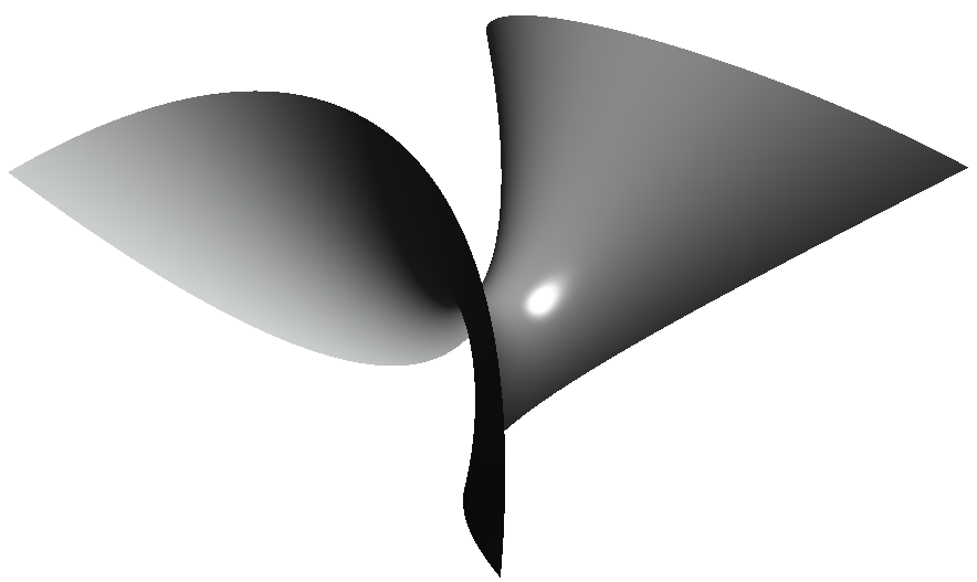
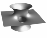
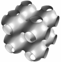
Figure 7.10: From the left, the minimal surfaces of Enneper, Costa and Schwarz.

Theorem 52.

The non-planar points of a minimal surface are hyperbolic.

Proof.

This is a direct consequence of the definition of mean curvature $H$ and of hyperbolic points: $H=0\iff\kappa_{1}\kappa_{2}<0$. ∎

Let $\mathbf{f}:\Omega\rightarrow\Sigma$ be a regular surface and $Q$ a subset of $\Omega$ with its boundary $\partial Q$ a closed regular curve in $\Omega$; then, $R=\mathbf{f}(Q)\subset\Sigma$ is a simple region of $\Sigma$. Let $h:Q\rightarrow\mathbb{R}$ be a smooth function. Then, we call normal variation of R the map $\boldsymbol{\varphi}:Q\times(-\epsilon,\epsilon)\rightarrow\mathcal{E}$ defined by

$$\boldsymbol{\varphi}(u,v,t)=\mathbf{f}(u,v)+t\ h(u,v)\mathbf{N}(u,v).$$

For each fixed $t$, $\boldsymbol{\varphi}(u,v,t)$ is a surface with

$$\begin{split}&\boldsymbol{\varphi}_{,u}(u,v,t)=\mathbf{f}_{,u}(u,v)+t\ h(u,v)\mathbf{N}_{,u}(u,v)+t\ h_{,u}(u,v)\mathbf{N}(u,v),\\ &\boldsymbol{\varphi}_{,v}(u,v,t)=\mathbf{f}_{,v}(u,v)+t\ h(u,v)\mathbf{N}_{,v}(u,v)+t\ h_{,v}(u,v)\mathbf{N}(u,v).\end{split}$$

If the first fundamental form of $\mathbf{f}$ is represented by the metric tensor $\mathbf{g}$, we look for the metric tensor $\mathbf{g}^{t}$ representing the first fundamental form of $\boldsymbol{\varphi}(u,v,t)\ \forall t$:

$$\begin{split}&g_{11}^{t}=\boldsymbol{\varphi}_{,u}\cdot\boldsymbol{\varphi}_{,u}=g_{11}+2t\ h\ \mathbf{f}_{,u}\cdot\mathbf{N}_{,u}+t^{2}(h^{2}\mathbf{N}_{,u}^{2}+h_{,u}^{2}),\\ &g_{12}^{t}=\boldsymbol{\varphi}_{,u}\cdot\boldsymbol{\varphi}_{,v}=g_{12}+t\ h(\mathbf{f}_{,u}\cdot\mathbf{N}_{,v}+\mathbf{f}_{,v}\cdot\mathbf{N}_{,u})+t^{2}(h^{2}\mathbf{N}_{,u}\cdot\mathbf{N}_{,v}+h_{,u}h_{,v}),\\ &g_{22}^{t}=\boldsymbol{\varphi}_{,v}\cdot\boldsymbol{\varphi}_{,v}=g_{22}+2t\ h\ \mathbf{f}_{,v}\cdot\mathbf{N}_{,v}+t^{2}(h^{2}\mathbf{N}_{,v}^{2}+h_{,v}^{2}),\end{split}$$

and by Eq. (7.14),

$$\begin{split}&g_{11}^{t}=g_{11}-2t\ h\ B_{11}+t^{2}(h^{2}\mathbf{N}_{,u}^{2}+h_{,u}^{2}),\\ &g_{12}^{t}=g_{12}-2t\ h\ B_{12}+t^{2}(h^{2}\mathbf{N}_{,u}\cdot\mathbf{N}_{,v}+h_{,u}h_{,v}),\\ &g_{22}^{t}=g_{22}-2t\ h\ B_{22}+t^{2}(h^{2}\mathbf{N}_{,v}^{2}+h_{,v}^{2}),\end{split}$$

whence

$$\det\mathbf{g}^{t}=\det\mathbf{g}-2th(g_{11}B_{22}-2g_{12}B_{12}+g_{22}B_{11})+o(t^{2}).$$

Then, by Eq. (7.15), we get easily that

$$g_{11}B_{22}-2g_{12}B_{12}+g_{22}B_{11}=2H\det\mathbf{g},$$

so that

$$\det\mathbf{g}^{t}=\det\mathbf{g}(1-4thH)+o(t^{2}).$$

We can now calculate the area $\mathcal{A}(t)$of the simple region $R^{t}=\boldsymbol{\varphi}(u,v,t)$ corresponding to the subset $Q$:

$$\mathcal{A}^{t}=\int_{Q}\sqrt{\det\mathbf{g}(1-4thH)+o(t^{2})}dudv;$$

For $\epsilon\ll 1\ \mathcal{A}^{t}$ is differentiable and its derivative for $t=0$ is

$$\left[\frac{d\mathcal{A}^{t}}{dt}\right]_{t=0}=-\int_{Q}2hH\sqrt{\det\mathbf{g}}dudv.$$

Theorem 53.

A surface $\mathbf{f}:\Omega\rightarrow\Sigma$ is minimal $\iff\left[\dfrac{d\mathcal{A}^{t}}{dt}\right]_{t=0}=0\ \ \forall R\subset\Sigma$ and for each normal variation.

Proof.

If $\mathbf{f}$ is minimal, the condition is clearly satisfied ($H=0$). Conversely, let us suppose that $\exists p=\mathbf{f}(\overline{u},\overline{v})\in\Sigma|H(p)\neq 0$. Consider $r_{1},r_{2}\in\mathbb{R}$ such that $|H|\neq 0$ in the circle $D_{2}$ with center $p$ and radius $r_{2}$ and $|H|>\frac{1}{2}|H(p)|$ in the circle $D_{1}$ with center $p$ and radius $r_{1}$. Then, we chose a smooth function $h(u,v)$ such that $i)\ h=H$ inside $D_{1}$, $ii)\ hH>0$ inside $D_{2}$ and $iii)\ h=0$ outside $D_{2}$. For the normal variation defined by such $h(u,v)$ we have

$$\begin{split}-\left[\frac{d\mathcal{A}^{t}}{dt}\right]_{t=0}&=\int_{D_{2}}2hH\sqrt{\det\mathbf{g}}du\ dv\geq\int_{D_{1}}2H^{2}\sqrt{\det\mathbf{g}}du\ dv\\ &\geq\int_{D_{1}}\frac{H(p)^{2}}{2}\sqrt{\det\mathbf{g}}du\ dv=\frac{H(p)^{2}}{2}\mathcal{A}(\mathbf{f}(D_{1}))\\ &\Rightarrow\left[\dfrac{d\mathcal{A}^{t}}{dt}\right]_{t=0}<0\end{split}$$

which contradicts the hypothesis. ∎

The meaning of this theorem justifies the name of minimal surfaces: These are the surfaces that have the minimal area among all the surfaces that share the same boundary.

7.16 Geodesics

Let $\mathbf{f}:\Omega\rightarrow\Sigma$ be a surface and $\boldsymbol{\gamma}(t):G\subset\mathbb{R}\rightarrow\Sigma$ a curve on $\Sigma$. A vector function $\mathbf{w}(t):G\rightarrow T_{\boldsymbol{\gamma}(t)}\Sigma$ is called a vector field along $\boldsymbol{\gamma}(t)$. We call covariant derivative of $\mathbf{w}(t)$ along $\boldsymbol{\gamma}(t)$ the vector field $D_{\boldsymbol{\gamma}}\mathbf{w}(t):G\rightarrow\mathcal{V}$ defined as

$$D_{\boldsymbol{\gamma}}\mathbf{w}:=(\mathbf{I}-\mathbf{N}\otimes\mathbf{N})\frac{d\mathbf{w}}{dt},$$

i.e. the projection of the derivative of $\mathbf{w}$ onto $T_{\boldsymbol{\gamma}(t)}\Sigma$. It is always possible to decompose $\mathbf{w}(t)$ into its components in the natural basis $\{\mathbf{f}_{,u},\mathbf{f}_{,v}\}$:

$$\mathbf{w}(t)=w_{1}(t)\mathbf{f}_{,u}(\boldsymbol{\gamma}(t))+w_{2}(t)\mathbf{f}_{,v}(\boldsymbol{\gamma}(t)).$$

Differentiating, we get (a prime here denotes the derivative with respect to $t$)

$$\mathbf{w}^{\prime}=w^{\prime}_{1}\mathbf{f}_{,u}+w_{1}(\mathbf{f}_{,uu}u^{\prime}+\mathbf{f}_{,uv}v^{\prime})+w^{\prime}_{2}\mathbf{f}_{,v}+w_{2}(\mathbf{f}_{,uv}u^{\prime}+\mathbf{f}_{,vv}v^{\prime})$$

and using the Gauss equations, Eq. (7.25)₁, we obtain (summation on the dummy indexes and $u_{1}$ stands for $u$ while $u_{2}$ for $v$)

$$\mathbf{w}^{\prime}=\mathbf{f}_{,k}w^{\prime}_{k}+(\Gamma^{k}_{ij}\mathbf{f}_{,k}+B_{ij}\mathbf{N})w_{i}u^{\prime}_{j},\ \ \ i,j,k=1,2,$$

so that the projection onto $T_{\boldsymbol{\gamma}(t)}\Sigma$, i.e. $D_{\boldsymbol{\gamma}}\mathbf{w}(t)$, is

$$D_{\boldsymbol{\gamma}}\mathbf{w}=(w^{\prime}_{k}+\Gamma^{k}_{ij}w_{i}u^{\prime}_{j})\mathbf{f}_{,k}.$$ (7.30)

A parallel vector field $\mathbf{w}$ along $\boldsymbol{\gamma}$ is a vector field having $\mathbf{D}_{\boldsymbol{\gamma}}\mathbf{w}=\mathbf{o}\ \forall t$. A regular curve $\boldsymbol{\gamma}$ is a geodesic of $\Sigma$ if the vector field $\boldsymbol{\gamma}^{\prime}$ of the vectors tangent to $\boldsymbol{\gamma}$ is parallel along $\boldsymbol{\gamma}$.

Theorem 54.

A curve $\boldsymbol{\gamma}$ is a geodesic of $\Sigma\iff\boldsymbol{\nu}\times\mathbf{N}=\mathbf{o}$.

Proof.

If $\boldsymbol{\gamma}$ is a geodesic, then the derivative of its tangent $\boldsymbol{\gamma}^{\prime}$ has a component only along $\mathbf{N}$, i.e. $\boldsymbol{\gamma}^{\prime\prime}\times\mathbf{N}=\mathbf{o}\Rightarrow\boldsymbol{\gamma}^{\prime}\cdot\boldsymbol{\gamma}^{\prime\prime}=0$. The principal normal to $\boldsymbol{\gamma}$, $\boldsymbol{\nu}$, is orthogonal to $\boldsymbol{\gamma}^{\prime}\Rightarrow\boldsymbol{\nu}\times\mathbf{N}=\mathbf{o}$. Vice versa, if $\boldsymbol{\nu}\times\mathbf{N}=\mathbf{o}$, then $\boldsymbol{\gamma}^{\prime\prime}$ is orthogonal to $\boldsymbol{\gamma}^{\prime}\Rightarrow\mathbf{D}_{\boldsymbol{\gamma}}\boldsymbol{\gamma}^{\prime}=\mathbf{o}$, i.e. $\boldsymbol{\gamma}$ is a geodesic. ∎

Theorem 55.

If $\boldsymbol{\gamma}$ is a geodesic, then $|\boldsymbol{\gamma}^{\prime}|=const.$

Proof.

In a geodesic, $\boldsymbol{\gamma}^{\prime}\cdot\boldsymbol{\gamma}^{\prime\prime}=0\Rightarrow\dfrac{d(\boldsymbol{\gamma}^{\prime}\cdot\boldsymbol{\gamma}^{\prime})}{dt}=0\Rightarrow|\boldsymbol{\gamma}^{\prime}|=const.$ ∎

This result shows that, in a geodesic, the parameter is always the natural parameter $s$.

Let $\boldsymbol{\gamma}(s)$ be a curve on $\Sigma$ parameterized by the the arc-length $s$. We call geodesic curvature of $\boldsymbol{\gamma}(s)$ the function

$$\kappa_{g}:=D_{\boldsymbol{\gamma}}\boldsymbol{\tau}\cdot(\mathbf{N}\times\boldsymbol{\tau}),$$

where $\boldsymbol{\tau}=\boldsymbol{\gamma}^{\prime}\in\mathcal{S}$ is the tangent vector to $\boldsymbol{\gamma}$. Because $\mathbf{N}\times\boldsymbol{\tau}\in\mathcal{S}$ lies in $T_{\boldsymbol{\gamma}}\Sigma$, the component of $\boldsymbol{\tau}^{\prime}$ orthogonal to $T_{\boldsymbol{\gamma}}\Sigma$ gives a null contribution to $\kappa_{g}$, so we can also write

$$\kappa_{g}=\boldsymbol{\tau}^{\prime}\cdot(\mathbf{N}\times\boldsymbol{\tau}).$$

Theorem 56.

A regular curve $\boldsymbol{\gamma}(s)$ is a geodesic $\iff\kappa_{g}=0\ \forall s$.

Proof.

If $\boldsymbol{\gamma}$ is a geodesic, clearly $\kappa_{g}=0$. Vice versa, if $\kappa_{g}=0$, then $\boldsymbol{\tau},\boldsymbol{\tau}^{\prime}$ and $\mathbf{N}$ are linearly dependent, i.e. coplanar. Because $\boldsymbol{\tau}^{\prime}\cdot\boldsymbol{\tau}=\mathbf{N}\cdot\boldsymbol{\tau}=0\Rightarrow\boldsymbol{\tau}^{\prime}\times\mathbf{N}=\mathbf{o}\Rightarrow$ by Theorem 54, $\boldsymbol{\gamma}$ is a geodesic. ∎

Let us now write Eq. (7.30) in the particular case of $\mathbf{w}=\boldsymbol{\gamma}^{\prime}$, i.e. $w_{1}=u^{\prime},w_{2}=v^{\prime}$:

$$D_{\boldsymbol{\gamma}}\mathbf{w}=(u^{\prime\prime}_{k}+\Gamma^{k}_{ij}u^{\prime}_{i}u^{\prime}_{j})\mathbf{f}_{,k};$$

therefore, the geodesics are the solutions to the system of differential equations

$$\left\{\begin{split}&u^{\prime\prime}+\Gamma^{1}_{11}u^{\prime 2}+2\Gamma^{1}_{12}u^{\prime}v^{\prime}+\Gamma^{1}_{22}v^{\prime 2}=0,\\ &v^{\prime\prime}+\Gamma^{2}_{11}u^{\prime 2}+2\Gamma^{2}_{12}u^{\prime}v^{\prime}+\Gamma^{2}_{22}v^{\prime 2}=0.\end{split}\right.$$ (7.31)

It can be shown that $\forall p\in\Sigma$ and $\forall\mathbf{w}(p)\in T_{p}\Sigma$ the geodesic is unique.

Let $p$ be a point of a regular surface $\mathbf{f}:\Omega\rightarrow\Sigma$ and $\boldsymbol{\alpha}(v):G\subset\mathbb{R}\rightarrow\Sigma$ a smooth regular curve on $\Sigma$, with $v$ being the natural parameter and such that $p=\boldsymbol{\alpha}(0)$. Consider the geodesic $\boldsymbol{\gamma}_{v}$ passing through $q=\boldsymbol{\alpha}(v)$ and such that $\boldsymbol{\gamma}^{\prime}_{v}(0)=\mathbf{N}(\boldsymbol{\alpha}(v))\times\boldsymbol{\tau}(v)$, with $\boldsymbol{\tau}(v)$ the (unit) tangent vector to $\boldsymbol{\alpha}(v)$. Consider the map $\mathbf{f}(u,v):\Omega\rightarrow\Sigma$ defined by posing $\mathbf{f}(u,v)=\boldsymbol{\gamma}_{v}(u)$; this is a surface whose coordinates $(u,v)$ are called semigeodesic coordinates.

Let us see the form that the first fundamental form (i.e. the metric tensor $\mathbf{g}$), the Christoffel symbols and the Gaussian curvature take in semigeodesic coordinates. Curves $\mathbf{f}(u,v_{0})=\boldsymbol{\gamma}_{v_{0}}(u)$ are geodesics, and $u$ is hence their natural parameter. Therefore, $\mathbf{f}_{,u}\in\mathcal{S}\Rightarrow g_{11}=1$. Then, $\mathbf{f}_{,uu}(u,v_{0})$ is the derivative of the tangent vector to a geodesic $\mathbf{f}(u,v_{0})=\boldsymbol{\gamma}_{v_{0}}(u)\Rightarrow\mathbf{f}_{,uu}(u,v_{0})$ does not have a component along the tangent, hence, Eq. (7.26)${}_{1}\Rightarrow\Gamma^{1}_{11}=\Gamma^{2}_{11}=0.$ Then, by Eq. (7.26)₂, we get $g_{12,u}=0\Rightarrow g_{12}$ does not depend upon $u\Rightarrow g_{12}(u,v)=g_{12}(0,v)\ \forall u$. Moreover, let $\theta$ be the angle between the curve $\boldsymbol{\alpha}$, i.e. between the coordinate line $\mathbf{f}(0,v)$, whose tangent vector is $\mathbf{f}_{,v}(0,v)$, and the geodesic $\boldsymbol{\gamma}_{v}(u)$, whose tangent vector at $(0,v)$ is $\boldsymbol{\gamma}^{\prime}_{v}(u)$. Then, $\theta=\dfrac{\pi}{2}$ because $\boldsymbol{\gamma}^{\prime}_{v}(0)=\mathbf{N}(\boldsymbol{\alpha}(v))\times\boldsymbol{\tau}(v)$. As a consequence, $g_{12}(0,v)=0\Rightarrow g_{12}(u,v)=0\ \forall(u,v)\in\Omega$. Finally, setting $\mathbf{g}_{22}=g$,

$$\mathbf{g}=\left[\begin{array}[]{cc}1&0\\ 0&g\end{array}\right],$$

with $g>0$ because $\mathbf{g}$ is positive definite. Through systems (7.26)$-$(7.28), we obtain

$$\Gamma^{1}_{12}=0,\ \ \Gamma^{2}_{12}=\frac{g_{,u}}{2g},\ \ \Gamma^{1}_{22}=-\frac{g_{,u}}{2},\ \ \Gamma^{2}_{22}=\frac{g_{,v}}{2g},$$

and using Eq. (7.29), we get

$$K=\det\mathbf{X}=-\frac{g_{,uu}}{2g}+\frac{g^{2}_{,u}}{4g^{2}}.$$

Given two points $p_{1},p_{2}\in\Sigma$, we define the distance $d(p_{1},p_{2})$ as the infimum of the lengths of the curves on $\Sigma$ joining the two points. We end with an important characterization of geodesics:

Theorem 57.

Geodesics are the curves of minimal distance between two points of a surface.

Proof.

Let $\boldsymbol{\gamma}:G\subset\mathbb{R}\rightarrow\Sigma$ be a geodesic on $\Sigma$, parameterized with the arc-length, and $\boldsymbol{\alpha}$ a smooth regular curve through $p$ and orthogonal to $\boldsymbol{\gamma}$. Through $\boldsymbol{\alpha}$, we set up a system of semigeodesic coordinates in a neighbourhood $U$ of $p$. With an opportune parameterization $\boldsymbol{\alpha}(t)$, in such coordinates we can get $p=\mathbf{f}(0,0)$ and $\boldsymbol{\gamma}$ described by the equation $v=0$. Let $q\in U$ be a point in $\boldsymbol{\gamma}$, and consider a regular curve connecting $p$ with $q$. The length $\ell(p,q)$ of such a curve is

$$\ell(p,q)=\int_{p}^{q}\sqrt{u^{\prime 2}+g\ v^{\prime 2}}dt\geq\left|\int_{p}^{q}u^{\prime}dt\right|=|u_{q}-u_{p}|.$$

Observing that $p=(u_{p},0),q=(u_{q},0)$, we remark that $|u_{q}-u_{p}|$ is exactly the length of $\boldsymbol{\gamma}$ between $p$ and $q$, because $\boldsymbol{\gamma}$ is parameterized with its arc-length. ∎

There is another, direct and beautiful way to show that geodesics are the shortest path lines: the use of the methods of the calculus of variations. The length $\ell(p,q)$ of a curve $\boldsymbol{\gamma}(t)\in\Sigma$ between two points $p$ and $q$ is given by the functional (7.9); it depends upon the first fundamental form, i.e. upon the metric tensor $\mathbf{g}$ on $\Sigma$. For the sake of conciseness, let $\mathbf{w}=(w_{,t}^{1},w_{,t}^{2})$ be the tangent vector to the curve $\boldsymbol{\gamma}(w_{1},w_{2})\in\Sigma$. Then,

$$\ell(p,q)=\int_{p}^{q}\sqrt{I(\mathbf{w})}dt=\int_{p}^{q}\sqrt{\mathbf{w}\cdot\mathbf{g}\mathbf{w}}dt.$$

The curve $\boldsymbol{\gamma}(t)$ that minimizes $\ell(p,q)$ is the solution to the Euler-Lagrange equations

$$\frac{d}{dt}\frac{\partial F}{\partial\mathbf{w}_{,t}}-\frac{\partial F}{\partial\mathbf{w}}=\mathbf{o} \ \rightarrow\ \frac{d}{dt}\frac{\partial F}{\partial w^{k}_{,t}}-\frac{\partial F}{\partial w^{k}}=0,\ \ k=1,2,$$

where

$$F(\mathbf{w},\mathbf{w}_{,t},t)=\sqrt{\mathbf{w}\cdot\mathbf{g}\mathbf{w}}=\sqrt{g_{ij}w^{i}_{,t}w^{j}_{,t}}.$$

It is more direct, and equivalent, to minimize $J^{2}(t)$, i.e. to write the Euler-Lagrange equations for

$$\varPhi(\mathbf{w},\mathbf{w}_{,t},t):=F^{2}(\mathbf{w},\mathbf{w}_{,t},t)=g_{ij}w^{i}_{,t}w^{j}_{,t}.$$

Therefore:

$$\begin{split}&\frac{\partial\varPhi}{\partial w^{k}_{,t}}=2g_{jk}w^{j}_{,t},\\ &\frac{\partial\varPhi}{\partial w^{k}}=\frac{\partial g_{hj}}{\partial w^{k}}w^{h}_{,t}w^{j}_{,t},\\ &\frac{d}{dt}\frac{\partial\varPhi}{\partial w^{k}_{,t}}=2\left(g_{jk}w^{j}_{,tt}+\frac{dg_{jk}}{dt}w^{j}_{,t}\right)=2\left(g_{jk}w^{j}_{,tt}+\frac{\partial g_{jk}}{\partial w^{l}}w^{l}_{,t}w^{j}_{,t}\right),\end{split}\ \ \ \ j,h,k=1,2.$$

The Euler-Lagrange equations are hence

$$g_{jk}w^{j}_{,tt}+\frac{\partial g_{jk}}{\partial w^{h}}w^{h}_{,t}w^{j}_{,t}-\frac{1}{2}\frac{\partial g_{hj}}{\partial w^{k}}w^{h}_{,t}w^{j}_{,t}=0,,\ \ \ j,h,k=1,2,$$

which can be rewritten as

$$g_{jk}w^{j}_{,tt}+\frac{1}{2}\left(\frac{\partial g_{jk}}{\partial w^{h}}+\frac{\partial g_{hk}}{\partial w^{j}}-\frac{\partial g_{hj}}{\partial w^{k}}\right)w^{h}_{,t}w^{j}_{,t}=0,\ \ \ j,h,k=1,2.$$

Multiplying by $g^{lk}$, we get

$$g^{lk}g_{jk}w^{j}_{,tt}+\frac{1}{2}g^{lk}\left(\frac{\partial g_{jk}}{\partial w^{h}}+\frac{\partial g_{hk}}{\partial w^{j}}-\frac{\partial g_{hj}}{\partial w^{k}}\right)w^{h}_{,t}w^{j}_{,t}=0,\ \ \ j,h,k,l=1,2.$$

and finally, because

$$g^{lk}g_{jk}=\delta_{lj}$$

and by Eq. (6.26), we get

$$w^{l}_{,tt}+\Gamma^{l}_{jh}w^{j}_{,t}w^{h}_{,t}=0,\ \ \ j,h,l=1,2.$$

These are the differential equations whose solution is the curve of minimal length between two points of $\Sigma$; comparing these equations with those of a geodesic of $\Sigma$, Eq. (7.31), we see that they are the same: The geodesics of a surface are hence the curves of minimal distance on the surface.

The Christoffel symbols of a plane are all null; as a consequence, the geodesic lines of a plane are straight lines. In fact, only such lines have a constant derivative.

Through systems (7.26)$-$(7.28), we can calculate the Christoffel symbols for a revolution surface, Eq. (7.5), which are all null excepted

$$\Gamma^{2}_{12}=\frac{\varphi^{\prime}}{\varphi},\ \ \ \Gamma^{1}_{22}=-\varphi\ \varphi^{\prime},$$

so the system of differential equations (7.31) becomes

$$\left\{\begin{array}[]{l}u^{\prime\prime}-\varphi\ \varphi^{\prime}v^{\prime 2}=0,\\ v^{\prime\prime}+2\dfrac{\varphi^{\prime}}{\varphi}u^{\prime}v^{\prime}=0.\end{array}\right.$$ (7.32)

It is direct to check that the meridians $(u=t,v=v_{0})$ are geodesic lines, while the parallels $(u=u_{0},v=t)$ are geodesics $\iff\varphi^{\prime}(u_{0})=0$.

7.17 The Gauss-Codazzi compatibility conditions

Let us consider a surface $\Sigma$ whose points are determined by the vector function $\mathbf{r}:\Omega\subset\mathbb{R}^{2}\rightarrow\Sigma\subset\mathcal{E},\mathbf{r}(\alpha_{1},\alpha_{2})=x_{i}(\alpha_{1},\alpha_{2})\boldsymbol{\epsilon}_{i}$, with $\boldsymbol{\epsilon}_{i},i=1,2,3,$ the vectors of the orthonormal basis of the reference frame $\mathcal{R}=\{o;\boldsymbol{\epsilon}_{1},\boldsymbol{\epsilon}_{2},\boldsymbol{\epsilon}_{3}\}$ and the parameters $\alpha_{1},\alpha_{2}$ chosen in such a way that the lines $\alpha_{1}=const.,\alpha_{2}=const.$ are lines of curvature, i.e. tangent at each point to the principal directions of curvature and hence mutually orthogonal. With such a choice, cf. Eq. (7.8),

$$ds^{2}=A_{1}^{2}d\alpha_{1}^{2}+A_{2}^{2}d\alpha_{2}^{2},$$

with

$$\begin{split}&A_{1}=\sqrt{\mathbf{r}_{,\alpha_{1}}^{2}}=\sqrt{\frac{dx_{i}}{d\alpha_{1}}\frac{dx_{i}}{d\alpha_{1}}},\\ &A_{2}=\sqrt{\mathbf{r}_{,\alpha_{2}}^{2}}=\sqrt{\frac{dx_{i}}{d\alpha_{2}}\frac{dx_{i}}{d\alpha_{2}}}\end{split}$$

the so-called Lamé’s parameters. We remark that along the lines of curvatures, i.e. the lines $\alpha_{i}=const.,i=1,2$, which in short, from now, on we call the lines $\alpha_{i}$, it is

$$\begin{split}&ds_{1}=A_{1}d\alpha_{1},\\ &ds_{2}=A_{2}d\alpha_{2},\end{split}$$

and hence,

$$\begin{split}\boldsymbol{\lambda}_{1}=\frac{ds_{1}}{d\alpha_{1}}=A_{1}\mathbf{e}_{1},\\ \boldsymbol{\lambda}_{2}=\frac{ds_{2}}{d\alpha_{2}}=A_{2}\mathbf{e}_{2}\end{split}$$ (7.33)

are the vectors tangent to the lines of curvature. Let

$$\mathbf{e}_{1}=\frac{1}{A_{1}}\mathbf{r}_{,\alpha_{1}},\ \ \mathbf{e}_{2}=\frac{1}{A_{2}}\mathbf{r}_{,\alpha_{2}},\ \ \mathbf{e}_{3}=\mathbf{e}_{1}\times\mathbf{e}_{2}(=\mathbf{N});$$ (7.34)

these three vectors form the orthonormal (local) natural basis $\texttt{e}=\{\mathbf{e}_{1},\mathbf{e}_{2},\mathbf{e}_{3}\}$. We always make the choice of $\alpha_{1},\alpha_{2}$ such that $\mathbf{e}_{3}$ is always directed toward the convex side of $\Sigma$ if the point is elliptic or parabolic or toward the side of the centres of negative curvature, if the point is hyperbolic.

We consider a vector $\mathbf{v}=\mathbf{v}(p),\ p\in\Sigma$,

$$\mathbf{v}=v_{1}\mathbf{e}_{1}+v_{2}\mathbf{e}_{2}+v_{3}\mathbf{e}_{3},$$

and we want to calculate how it transforms when $p$ changes. To this end, we need to calculate how $\mathbf{e}_{1},\mathbf{e}_{2},\mathbf{e}_{3}$ change with $\alpha_{1},\alpha_{2}$. Let $q\in\Sigma$ be a point in the neighborhood of $p$ on the line $\alpha_{i}$ and let us first consider the change of $\mathbf{e}_{3}$ in passing from $p$ to $q$. Because $p$ and $q$ belong to the same line $\alpha_{i}$, by the theorem of Rodrigues, we get (no summation on $i$ in the following equations)

$$\frac{\partial\mathbf{e}_{3}}{\partial\boldsymbol{\lambda}_{i}}=-\kappa_{i}\boldsymbol{\lambda}_{i},\ i=1,2,$$

i.e., by Eq. (7.33),

$$\frac{\partial\mathbf{e}_{3}}{\partial\alpha_{i}}=\frac{A_{i}}{R_{i}}\mathbf{e}_{i},$$

with

$$R_{i}=-\frac{1}{\kappa_{i}}$$

the (principal) radius of curvature along the line $\alpha_{i}$. The minus sign in the previous equation is due to the choice made above for orienting $\mathbf{e}_{3}=\mathbf{N}$, which gives always $\mathbf{N}=-\boldsymbol{\nu}$, with $\boldsymbol{\nu}$ the principal normal to the line $\alpha_{i}$. This result can also be obtained directly, see Fig. 7.11:

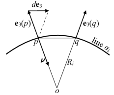
Figure 7.11: Variation of $\mathbf{N}=\mathbf{e}_{3}$ along a line of curvature.

$$\mathbf{e}_{3}(q)=\mathbf{e}_{3}(p)+d\mathbf{e}_{3}$$

and in the limit of $q\rightarrow p$, $d\mathbf{e}_{3}$ tends to be parallel to $q-p$ and

$$\lim_{q\rightarrow p}(q-p)=\boldsymbol{\lambda}_{i}=A_{i}\mathbf{e}_{i}.$$

By the similitude of the triangles, it is evident that

$$\frac{|d\mathbf{e}_{3}|}{|\mathbf{e}_{3}|}=\frac{|q-p|}{R_{i}};$$

moreover,

$$d\mathbf{e}_{3}=\frac{\partial\mathbf{e}_{3}}{\partial\alpha_{i}}d\alpha_{i}\mathbf{e}_{i}.$$

Finally, as $|\mathbf{e}_{3}|=1$, we get again

$$\frac{\partial\mathbf{e}_{3}}{\partial\alpha_{i}}=\frac{A_{i}}{R_{i}}\mathbf{e}_{i}.$$ (7.35)

Implicitly, in this last proof, we have used the theorem of Rodrigues because we have assumed that $d\mathbf{e}_{3}$ is parallel to $\boldsymbol{\lambda}_{i}$, as it is, because line $\alpha_{i}$ is a line of curvature.

We now move on to determine the changes in $\mathbf{e}_{1}$ and $\mathbf{e}_{2}$; for this purpose, we remark that

$$\frac{\partial\mathbf{r}_{,\alpha_{1}}}{\partial\alpha_{2}}=\frac{\partial^{2}\mathbf{r}}{\partial\alpha_{2}\partial\alpha_{1}}=\frac{\partial^{2}\mathbf{r}}{\partial\alpha_{1}\partial\alpha_{2}}=\frac{\partial\mathbf{r}_{,\alpha_{2}}}{\partial\alpha_{1}},$$

so by Eq. (7.34) we get

$$\frac{\partial(A_{1}\mathbf{e}_{1})}{\partial\alpha_{2}}=\frac{\partial(A_{2}\mathbf{e}_{2})}{\partial\alpha_{1}}.$$ (7.36)

Let us study now $\dfrac{\partial\mathbf{e}_{j}}{\partial\alpha_{i}}$; as $|\mathbf{e}_{j}|=1,j=1,2$,

$$\frac{\partial\mathbf{e}_{j}}{\partial\alpha_{i}}\cdot\mathbf{e}_{j}=0\ \ \forall i,j=1,2.$$ (7.37)

Because $\mathbf{e}_{1}\cdot\mathbf{e}_{2}=0$,

$$\frac{\partial\mathbf{e}_{1}}{\partial\alpha_{1}}\cdot\mathbf{e}_{2}=\frac{\partial(\mathbf{e}_{1}\cdot\mathbf{e}_{2})}{\partial\alpha_{1}}-\mathbf{e}_{1}\cdot\frac{\partial\mathbf{e}_{2}}{\partial\alpha_{1}}=-\mathbf{e}_{1}\cdot\frac{\partial\mathbf{e}_{2}}{\partial\alpha_{1}}.$$

By Eq. (7.36), we get

$$\frac{\partial\mathbf{e}_{2}}{\partial\alpha_{1}}=\frac{1}{A_{2}}\frac{\partial(A_{1}\mathbf{e}_{1})}{\partial\alpha_{2}}-\frac{1}{A_{2}}\frac{\partial A_{2}}{\partial\alpha_{1}}\mathbf{e}_{2},$$

which when inserted into the previous equation gives, by Eq. (7.37),

$$\frac{\partial\mathbf{e}_{1}}{\partial\alpha_{1}}\cdot\mathbf{e}_{2}=-\frac{1}{A_{2}}\frac{\partial(A_{1}\mathbf{e}_{1})}{\partial\alpha_{2}}\cdot\mathbf{e}_{1}+\frac{1}{A_{2}}\frac{\partial A_{2}}{\partial\alpha_{1}}\mathbf{e}_{2}\cdot\mathbf{e}_{1}=-\frac{A_{1}}{A_{2}}\frac{\partial\mathbf{e}_{1}}{\partial\alpha_{2}}\cdot\mathbf{e}_{1}-\frac{1}{A_{2}}\frac{\partial A_{1}}{\partial\alpha_{2}}\mathbf{e}_{1}\cdot\mathbf{e}_{1}=-\frac{1}{A_{2}}\frac{\partial A_{1}}{\partial\alpha_{2}}.$$

Then, because $\mathbf{e}_{1}\cdot\mathbf{e}_{3}=0$,

$$\frac{\partial\mathbf{e}_{1}}{\partial\alpha_{1}}\cdot\mathbf{e}_{3}=\frac{\partial(\mathbf{e}_{1}\cdot\mathbf{e}_{3})}{\partial\alpha_{1}}-\mathbf{e}_{1}\cdot\frac{\partial\mathbf{e}_{3}}{\partial\alpha_{1}}=-\mathbf{e}_{1}\cdot\frac{\partial\mathbf{e}_{3}}{\partial\alpha_{1}},$$

and by Eq. (7.35),

$$\frac{\partial\mathbf{e}_{3}}{\partial\alpha_{1}}=\frac{A_{1}}{R_{1}}\mathbf{e}_{1},$$

so finally,

$$\frac{\partial\mathbf{e}_{1}}{\partial\alpha_{1}}\cdot\mathbf{e}_{3}=-\frac{A_{1}}{R_{1}}.$$

Again, through Eqs. (7.36) and (7.37), we get

$$\frac{\partial\mathbf{e}_{1}}{\partial\alpha_{2}}\cdot\mathbf{e}_{2}=\frac{1}{A_{1}}\frac{\partial(A_{2}\mathbf{e}_{2})}{\partial\alpha_{1}}\cdot\mathbf{e}_{2}-\frac{1}{A_{1}}\frac{\partial A_{1}}{\partial\alpha_{2}}\mathbf{e}_{1}\cdot\mathbf{e}_{2}=\frac{A_{2}}{A_{1}}\frac{\partial\mathbf{e}_{2}}{\partial\alpha_{1}}\cdot\mathbf{e}_{2}+\frac{1}{A_{1}}\frac{\partial A_{2}}{\partial\alpha_{1}}\mathbf{e}_{2}\cdot\mathbf{e}_{2}=\frac{1}{A_{1}}\frac{\partial A_{2}}{\partial\alpha_{1}}$$

and also, by Eq. (7.35),

$$\frac{\partial\mathbf{e}_{1}}{\partial\alpha_{2}}\cdot\mathbf{e}_{3}=\frac{\partial(\mathbf{e}_{1}\cdot\mathbf{e}_{3})}{\partial\alpha_{2}}-\mathbf{e}_{1}\cdot\frac{\partial\mathbf{e}_{3}}{\partial\alpha_{2}}=-\mathbf{e}_{1}\cdot\frac{\partial\mathbf{e}_{3}}{\partial\alpha_{2}}=-\frac{A_{2}}{R_{2}}\mathbf{e}_{1}\cdot\mathbf{e}_{2}=0.$$

The derivatives of $\mathbf{e}_{2}$ can be found in a similar way, and resuming, we have

$$\begin{array}[]{ccl}\dfrac{\partial\mathbf{e}_{1}}{\partial\alpha_{1}}&=&-\dfrac{1}{A_{2}}\dfrac{\partial A_{1}}{\partial\alpha_{2}}\mathbf{e}_{2}-\dfrac{A_{1}}{R_{1}}\mathbf{e}_{3},\vskip 6.0pt plus 2.0pt minus 2.0pt\\ \dfrac{\partial\mathbf{e}_{1}}{\partial\alpha_{2}}&=&\dfrac{1}{A_{1}}\dfrac{\partial A_{2}}{\partial\alpha_{1}}\mathbf{e}_{2},\vskip 6.0pt plus 2.0pt minus 2.0pt\\ \dfrac{\partial\mathbf{e}_{2}}{\partial\alpha_{1}}&=&\dfrac{1}{A_{2}}\dfrac{\partial A_{1}}{\partial\alpha_{2}}\mathbf{e}_{1},\vskip 6.0pt plus 2.0pt minus 2.0pt\\ \dfrac{\partial\mathbf{e}_{2}}{\partial\alpha_{2}}&=&-\dfrac{1}{A_{1}}\dfrac{\partial A_{2}}{\partial\alpha_{1}}\mathbf{e}_{1}-\dfrac{A_{2}}{R_{2}}\mathbf{e}_{3},\vskip 6.0pt plus 2.0pt minus 2.0pt\\ \dfrac{\partial\mathbf{e}_{3}}{\partial\alpha_{1}}&=&\dfrac{A_{1}}{R_{1}}\mathbf{e}_{1},\vskip 6.0pt plus 2.0pt minus 2.0pt\\ \dfrac{\partial\mathbf{e}_{3}}{\partial\alpha_{2}}&=&\dfrac{A_{2}}{R_{2}}\mathbf{e}_{2}.\end{array}$$ (7.38)

Passing now to the second-order derivatives, imposing the equality of mixed derivatives, gives some important differential relations between the Lamé’s parameters $A_{i}$ and the radii of curvature $R_{i}$. In fact, from the identity

$$\frac{\partial^{2}\mathbf{e}_{3}}{\partial\alpha_{1}\partial\alpha_{2}}=\frac{\partial^{2}\mathbf{e}_{3}}{\partial\alpha_{2}\partial\alpha_{1}},$$

and Eqs. (7.38)_5,6, we get

$$\frac{\partial}{\partial\alpha_{2}}\left(\dfrac{A_{1}}{R_{1}}\mathbf{e}_{1}\right)=\frac{\partial}{\partial\alpha_{1}}\left(\dfrac{A_{2}}{R_{2}}\mathbf{e}_{2}\right),$$

whence

$$\frac{\partial}{\partial\alpha_{2}}\left(\dfrac{A_{1}}{R_{1}}\right)\mathbf{e}_{1}+\dfrac{A_{1}}{R_{1}}\frac{\partial\mathbf{e}_{1}}{\partial\alpha_{2}}=\frac{\partial}{\partial\alpha_{1}}\left(\dfrac{A_{2}}{R_{2}}\right)\mathbf{e}_{2}+\dfrac{A_{2}}{R_{2}}\frac{\partial\mathbf{e}_{2}}{\partial\alpha_{1}}.$$

Inserting now Eqs. (7.38)_2,3 into the last result and rearranging the terms gives

$$\left[\frac{\partial}{\partial\alpha_{2}}\left(\dfrac{A_{1}}{R_{1}}\right)-\frac{1}{R_{2}}\frac{\partial A_{1}}{\partial\alpha_{2}}\right]\mathbf{e}_{1}-\left[\frac{\partial}{\partial\alpha_{1}}\left(\dfrac{A_{2}}{R_{2}}\right)-\frac{1}{R_{1}}\frac{\partial A_{2}}{\partial\alpha_{1}}\right]\mathbf{e}_{2}=0,$$

that to be true needs that the two following conditions be identically satisfied:

$$\begin{split}&\frac{\partial}{\partial\alpha_{2}}\left(\dfrac{A_{1}}{R_{1}}\right)-\frac{1}{R_{2}}\frac{\partial A_{1}}{\partial\alpha_{2}}=0,\\ &\frac{\partial}{\partial\alpha_{1}}\left(\dfrac{A_{2}}{R_{2}}\right)-\frac{1}{R_{1}}\frac{\partial A_{2}}{\partial\alpha_{1}}=0.\end{split}$$ (7.39)

The above equations are known as the Codazzi conditions. Let us now consider the other identity

$$\frac{\partial^{2}\mathbf{e}_{1}}{\partial\alpha_{1}\partial\alpha_{2}}=\frac{\partial^{2}\mathbf{e}_{1}}{\partial\alpha_{2}\partial\alpha_{1}};$$

again using Eq. (7.38), with some standard operations, this identity can be transformed to

$$\left[\frac{\partial}{\partial\alpha_{1}}\left(\frac{1}{A_{1}}\frac{\partial A_{2}}{\partial\alpha_{1}}\right)+\frac{\partial}{\partial\alpha_{2}}\left(\frac{1}{A_{2}}\frac{\partial A_{1}}{\partial\alpha_{2}}\right)+\frac{A_{1}}{R_{1}}\frac{A_{2}}{R_{2}}\right]\mathbf{e}_{2}+\left[\frac{\partial}{\partial\alpha_{2}}\left(\frac{A_{1}}{R_{1}}\right)-\frac{1}{R_{2}}\frac{\partial A_{1}}{\partial\alpha_{2}}\right]\mathbf{e}_{3}=0.$$

Also in this case, for this equation to be identically satisfied, each of the expressions in square brackets must vanish, which gives two more differential conditions, but of which only the first one is new, as the second one corresponds to Eq. (7.39)₁. The new condition is hence

$$\frac{\partial}{\partial\alpha_{1}}\left(\frac{1}{A_{1}}\frac{\partial A_{2}}{\partial\alpha_{1}}\right)+\frac{\partial}{\partial\alpha_{2}}\left(\frac{1}{A_{2}}\frac{\partial A_{1}}{\partial\alpha_{2}}\right)+\frac{A_{1}}{R_{1}}\frac{A_{2}}{R_{2}}=0,$$ (7.40)

which is known as the Gauss condition. The last identity

$$\frac{\partial^{2}\mathbf{e}_{2}}{\partial\alpha_{1}\partial\alpha_{2}}=\frac{\partial^{2}\mathbf{e}_{2}}{\partial\alpha_{2}\partial\alpha_{1}}$$

does not add any independent condition, which can be easily checked. The meaning of the Gauss-Codazzi conditions, Eqs. (7.39) and (7.40), is that of compatibility conditions: Only when these conditions are satisfied by functions $A_{1},A_{2},R_{1}$ and $R_{2}$, then such functions represent the Lamé’s parameters and the principal radii of curvature of a surface, i.e. only in this case they define a surface, except for its position in space. The Gauss-Codazzi conditions are important in establishing the equations of the classical theory of shells.

7.18 Exercises

1. Prove that a function of the type $x_{3}=f(x_{1},x_{2})$, with $f:\Omega\subset\mathbb{R}^{2}\rightarrow\mathbb{R}$ smooth, defines a surface.

2. Show that the catenoid is the rotation surface of a catenary, then find its Gaussian curvature.

3. Show that the pseudo-sphere is the rotation surface of a tractrice and explain why the surface has this name (hint: look for its Gaussian curvature).

4. Prove that the regularity of a cone $\mathbf{f}(u,v)=v\boldsymbol{\gamma}(u)$ is satisfied at each point except at the apex and at the points on the straight lines tangent to $\boldsymbol{\gamma}(u)$.

   

   

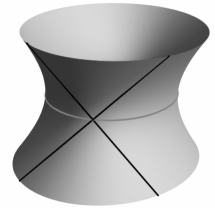
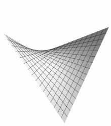
   Figure 7.12: A hyperbolic hyperboloid, left, and a hyperbolic paraboloid, right.

5. Prove that the hyperbolic hyperboloid is a doubly ruled surface and determine the angle $\theta$ formed by two straight lines belonging to the two sets of lines on the surface, see the left panel of Fig. 7.12.

6. Prove that the hyperbolic paraboloid whose Cartesian equation is $x_{3}=x_{1}x_{2}$, right panel of Fig. 7.12, is a doubly ruled surface and determine the angle $\theta$ formed by two straight lines belonging to the two sets of lines on the surface. Where does $\theta=\dfrac{\pi}{2}$?

7. Consider the parameterization

   $$\mathbf{f}(u,v)=(1-v)\boldsymbol{\gamma}(u)+v\boldsymbol{\lambda}(u),$$

   with

   $$\boldsymbol{\gamma}(u)=(\cos(u-\alpha),\sin(u-\alpha),-1),\ \ \boldsymbol{\lambda}(u)=(\cos(u+\alpha),\sin(u+\alpha),1).$$

   Show that:

   • for $\alpha=0$, one gets a cylinder with equation $x_{1}^{2}+x_{2}^{2}=1$;

   • for $\alpha=\dfrac{\pi}{2}$, one gets a cone with equation $x_{1}^{2}+x_{2}^{2}=x_{3}^{2}$;

   • for $0<\alpha<\dfrac{\pi}{2}$, one gets a hyperbolic hyperboloid with equation

     $$\dfrac{x_{1}^{2}+x_{2}^{2}}{\cos^{2}\alpha}-\dfrac{x_{3}^{2}}{\cot^{2}\alpha}=1.$$

8. Calculate the metric tensor of a sphere of radius $R$, write its first fundamental form, determine the area of a sector of surface between the longitudes $\theta_{1}$ and $\theta_{2}$ and the length of the parallel at the latitude $\pi/4$ between these two longitudes.

9. Prove that the surface defined by

   $$\mathbf{f}(u,v):\Omega=\mathbb{R}\times(-\pi,\pi]\rightarrow\mathcal{E}|\ \ \mathbf{f}(u,v)=\left(\frac{\cos v}{\cosh u},\frac{\sin v}{\cosh u},\frac{\sinh u}{\cosh u}\right)$$

   is a sphere. Then, show that the image of any straight line on $\Omega$ is a loxodromic line on the sphere.

10. Calculate the vectors of the natural basis, the tensors $\mathbf{g},\mathbf{B},\mathbf{X}$ and the first and second fundamental forms for the catenoid.

11. Calculate the same for the helicoid of parametric equation

    $$\mathbf{f}(u,v)=\boldsymbol{\gamma}(u)+v\boldsymbol{\lambda}(u),$$

    with

    $$\boldsymbol{\gamma}(u)=(0,0,u),\ \ \boldsymbol{\lambda}(u)=(\cos u,\sin u,0).$$

12. Show that the catenoid and the helicoid are made of hyperbolic points.

13. Determine the geodesic lines of a circular cylinder.

Suggested texts

There are many textbooks on tensors, differential geometry and calculus of variations. The style, content, language of such books greatly depend upon the scientific community the authors belong to: pure or applied mathematicians, physicists, theoretical mechanicians or engineers. It is hence difficult to suggest some readings in the domain, and ultimately, it is mostly a matter of personal taste.

This textbook is greatly inspired by some classical methods, style and language that are typical in the community of theoretical mechanics; the following few suggested readings, among several possible others, belong to such a kind of scientific literature. They are classical textbooks and though the list is far from being exhaustive, they constitute a solid basis for the topics briefly developed in this manuscript, where the objective is to present mathematics for mechanics.

A good introduction to tensor algebra and analysis, which greatly inspired the content of this manuscript, are the two introductory chapters of the classical textbook

• M. E. Gurtin: An introduction to continuum mechanics. Academic Press, 1981,

or also, in a similar style, the long article

• P. Podio-Guidugli: A primer in elasticity. Journal of Elasticity, v. 58: 1-104, 2000.

A short, effective introduction to tensor algebra and differential geometry of curves can be found in the following text of exercices on analytical mechanics:

• P. Biscari, C. Poggi, E. G. Virga: Mechanics notebook. Liguori Editore, 1999.

A classical textbook on linear algebra that is recommended is

• P. R. Halmos: Finite-dimensional vector spaces. Van Nostrand Reynold, 1958.

In the previous textbooks, tensor algebra in curvilinear coordinates is not developed; an introduction to this topic, especially intended for physicists and engineers, can be found in

• W. H. Müller: An expedition to continuum theory. Springer, 2014,

which has largely influenced Chapter 6.

Two modern and application-oriented textbooks on differential geometry of curves and surfaces are

• V. A. Toponogov: Differential geometry of curves and surfaces - A concise guide. Birkhäuser, 2006,

• A. Pressley: Elementary differential geometry. Springer, 2010.

A short introduction to the differential geometry of surfaces, oriented toward the mechanics of shells, can be found in the classical book

• V. V. Novozhilov: Thin shell theory. Noordhoff LTD., 1964.

For what concerns the calculus of variations, a still valid textbook in the matter (but not only) is

• R. Courant, D. Hilbert: Methods of mathematical physics. Interscience Publishers, 1953.

Two very good and classical textbooks with an introduction to the calculus of variations for engineers are

• C. Lanczos: The variational principles of mechanics. University of Toronto Press, 1949,

• H. L. Langhaar: Energy methods in applied mechanics. Wiley, 1962.