Power Generalized DUS Transformation of Exponential Distribution

Abstract

DUS transformation of lifetime distributions received attention by engineers and researchers in recent years. The present study introduces a new class of distribution using exponentiation of DUS transformation. A new distribution using the Exponential distribution as the baseline distribution in this transformation is proposed. The statistical properties of the proposed distribution have been examined and the parameter estimation is done using the method of maximum likelihood. The fitness of the proposed model is established using real data analysis.

1 Introduction

Modeling and analysis of lifetime distribution have been extensively used in many fields of science like engineering and statistics. Fitting of appropriate distribution is essential for a proper data anlysis. Different methods are available that propose new classes of distributions using existing distributions, see Gupta et al.[5], Nadarajah and Kotz[11], Cordeiro and Castro [1], Cordeiro et al.[2], Kumar et al.[8], etc. Kumar et al.[7] proposed a method called DUS transformation to obtain a new parsimonious class of distribution. Recently, Maurya et al.[10] proposed a generalization to DUS transformation to make it more flexible. Deepthi and Chacko[3] introduced DUS Lomax distribution. Gauthami and Chacko[4] introduced DUS Inverse Weibul distribution. But the existing approach is not appropriate for some data. A search for distributions with better fit is quite essential for data analysis in statistics and reliability engineering.

The current research work aims to introduce a new class of distribution using the exponentiation of DUS transformation, called Power generalized DUS (PGDUS) tranformation. The new PGDUS transformed distribution can be obtained as follows: Let X be a random variable with baseline cumulative distribution function (cdf) F(x) and corresponding probability density function (pdf) f(x). Then the cdf of the proposed PGDUS distribution is defined as,

$$G(x)=\left(\frac{e^{F(x)}-1}{e-1}\right)^{\theta},\theta>0,\,x>0.$$ (1)

and the corresponding pdf is,

$$g(x)=\frac{\theta}{(e-1)^{\theta}}(e^{F(x)}-1)^{\theta-1}e^{F(x)}f(x),\theta>0,\,x>0.$$ (2)

The associated survival function is,

$$S(x)=1-\big{(}\frac{e^{F(x)}-1}{e-1}\big{)}^{\theta},\theta>0,\,x>0.$$

The failure rate function is,

$$h(x)=\frac{\theta f(x)e^{F(x)}(e^{F(x)}-1)^{\theta-1}}{(e-1)^{\theta}-(e^{F(x)}-1)^{\theta}},\theta>0,\,x>0.$$

Application of the new transformation to the existing distributions has to be investigated. Using Exponential distribution as baseline distribution, Power Generalized DUS Exponential (PGDUSE) distribution is proposed, in this paper. It has to be studied in detail.

The rest of the paper is organized as follows. In Section 2, the PGDUSE is proposed. Sections 3 discussed the statistical properties of the proposed distribution. In Section 4, the maximum likelihood estimation procedure is applied for estimation of parameters. Real data set is analyzed in Section 5. Concluding remarks are given in Section 6.

2 Power Generalized DUS Exponential Distribution

Here, Power Generalized DUS transformation to the baseline distribution, Exponential distribution, is considered. Consider the Exponential distribution with parameter $\lambda$ as the baseline distribution. Invoking the PGDUS transformation given in equation(1), the cdf of the PGDUSE distribution is obtained as

$$G(x)=\bigg{(}\frac{e^{1-e^{-\lambda x}}-1}{e-1}\bigg{)}^{\theta},\lambda>0,\theta>0,x>0.$$ (3)

and the corresponding pdf is given by,

$$g(x)=\frac{\theta\lambda e^{1-\lambda x-e^{-\lambda x}}(e^{1-e^{-\lambda x}}-1)^{\theta-1}}{(e-1)^{\theta}},\lambda>0,\theta>0,x>0.$$ (4)

Then, the associated failure rate function is,

$$h(x)=\frac{\theta\lambda e^{1-\lambda x-e^{-\lambda x}}(e^{1-e^{-\lambda x}}-1)^{\theta-1}}{(e-1)^{\theta}-(e^{1-e^{-\lambda x}}-1)^{\theta}},\lambda>0,\theta>0,x>0.$$ (5)

We denote $PGDUSE(\lambda,\theta)$ for PGDUSE distribution with parameters $\lambda$ and $\theta$. Figure 1 shows that the density function of PGDUSE distribution is likely to be unimodal.

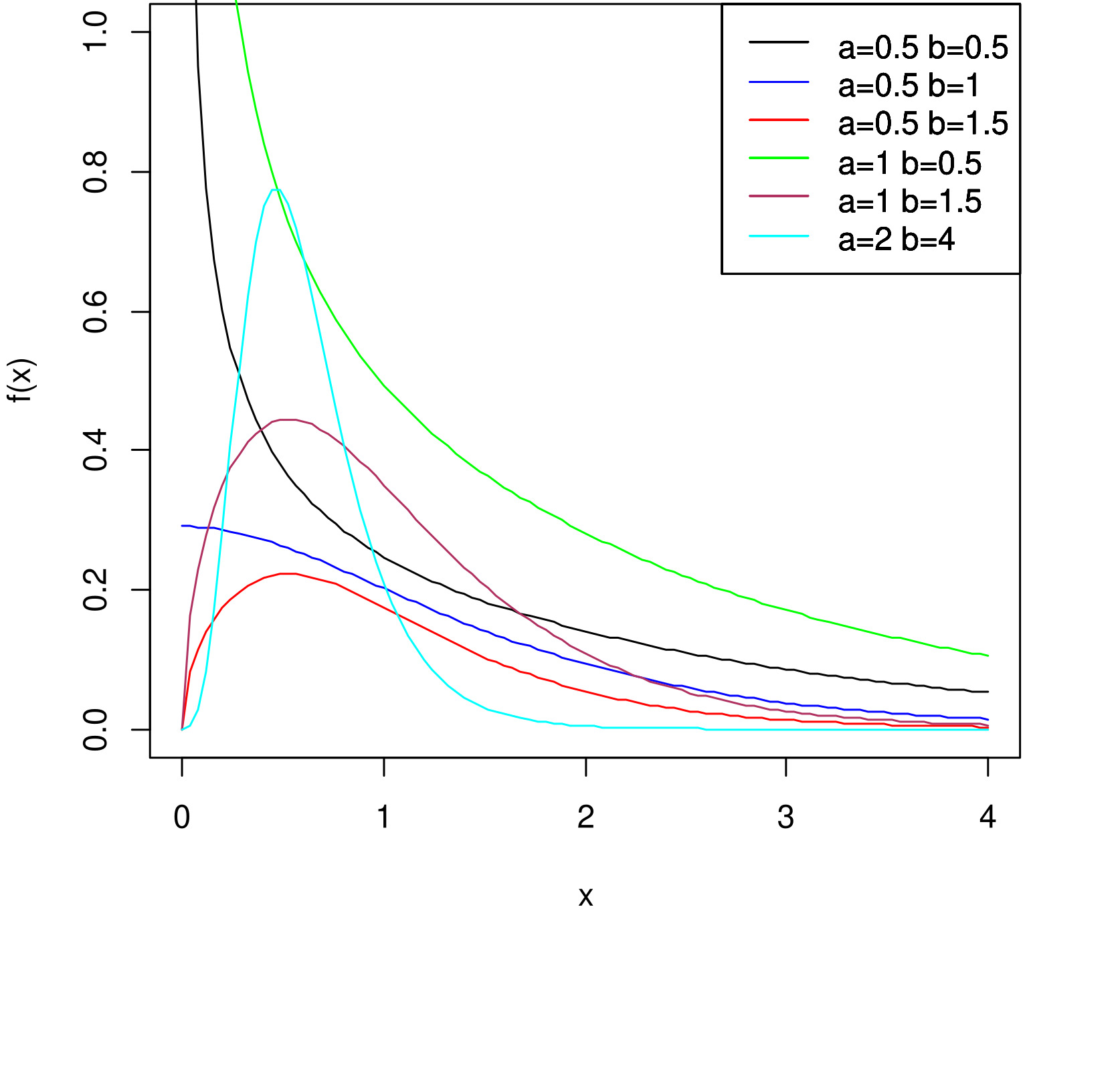
Figure 1: Density plot

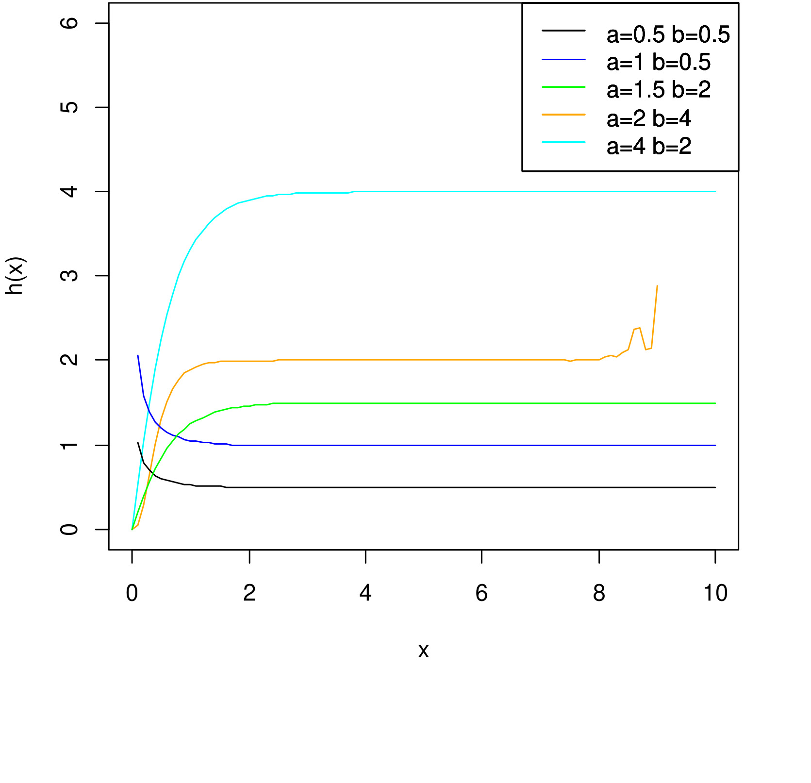
Figure 2: Failure rate plot

3 Statistical Properties

For a distribution, the statistical properties are inevitable. In this section, a few statistical properties like moments, moment generating function, characteristic function, cumulant generating function, quantile function, order statistics, and entropy of the proposed PGDUSE distribution are derived.

3.1 Moments

The rth raw moment of the $PGDUS-E(\lambda,\theta)$ distribution is given by

$$\mu^{\prime}_{r} =E(X^{r})$$

$$=\int_{0}^{\infty}x^{r}\frac{\theta\lambda}{(e-1)^{\theta}}e^{1-\lambda x-e^{-\lambda x}}(e^{1-e^{-\lambda x}}-1)dx$$

$$=\frac{\theta\lambda}{(e-1)^{\theta}}\int_{0}^{\infty}x^{r}e^{2-\lambda x-2e^{-\lambda x}}dx-\frac{\theta\lambda}{(e-1)^{\theta}}\int_{0}^{\infty}x^{r}e^{1-\lambda x-e^{-\lambda x}}dx$$

$$=\frac{\theta\lambda e^{2}}{(e-1)^{\theta}}\sum_{m=0}^{\infty}\frac{(-1)^{m}2^{m}r!}{m!(1+m)^{r+1}\lambda^{r+1}}-\frac{\theta\lambda e}{(e-1)^{\theta}}\sum_{m=0}^{\infty}\frac{(-1)^{m}r!}{m!(1+m)^{r+1}\lambda^{r+1}}$$

$$=\frac{\theta\lambda e}{(e-1)^{\theta}}\left[e\sum_{m=0}^{\infty}\frac{{(-1)^{m}}{2^{m}}}{m!(1+m)^{r+1}}-\sum_{m=0}^{\infty}\frac{(-1)^{m}}{m!(1+m)^{r+1}}\right]$$

By putting r=1, 2, 3… the raw moments can be viewed.

3.2 Moment Generating Function

The moment generating function (MGF) of $PGDUSE(\lambda,\theta)$ distribution is given by

$$M_{X}(t) =E(e^{tX})$$

$$=\int_{0}^{\infty}e^{tx}\frac{\theta\lambda}{(e-1)^{\theta}}e^{1-\lambda x-e^{-\lambda x}}(e^{1-e^{-\lambda x}}-1)dx$$

$$=\frac{\theta\lambda}{(e-1)^{\theta}}\int_{0}^{\infty}e^{tx-\lambda x-2e^{-\lambda x}}dx-\frac{\theta\lambda}{(e-1)^{\theta}}\int_{0}^{\infty}e^{1+tx-\lambda x-e^{-\lambda x}}dx$$

$$=\frac{\theta\lambda e^{2}}{(e-1)^{\theta}}\sum_{m=0}^{\infty}\frac{(-1)^{m}2^{m}}{m!(\lambda+\lambda m-t)}-\frac{\theta\lambda e}{(e-1)^{\theta}}\sum_{m=0}^{\infty}\frac{(-1)^{m}}{m!(\lambda+\lambda m-t)}$$

$$=\frac{\theta\lambda e}{(e-1)^{\theta}}\left[e\sum_{m=0}^{\infty}\frac{{(-1)^{m}}{2^{m}}}{m!(\lambda+\lambda m-t)}-\sum_{m=0}^{\infty}\frac{(-1)^{m}}{m!(\lambda+\lambda m-t)}\right]$$

3.3 Characteristic Function

The characteristic function (CF) is given by

$$\phi_{X}(t)=\frac{\theta\lambda e}{(e-1)^{\theta}}\left[e\sum_{m=0}^{\infty}\frac{{(-1)^{m}}{2^{m}}}{m!(\lambda+\lambda m-it)}-\sum_{m=0}^{\infty}\frac{(-1)^{m}}{m!(\lambda+\lambda m-it)}\right]$$

where $i=\sqrt{-1}$ is the unit imaginary number.

3.4 Cumulant Generating Function

The cumulant generating function (CGF) is given by

$$K_{X}(t) =\log\phi_{X}(t)=\log\left[\frac{\theta\lambda e}{(e-1)^{\theta}}\left[e\sum_{m=0}^{\infty}\frac{{(-1)^{m}}{2^{m}}}{m!(\lambda+\lambda m-it)}-\sum_{m=0}^{\infty}\frac{(-1)^{m}}{m!(\lambda+\lambda m-it)}\right]\right]$$

$$=\log(\frac{\theta\lambda e}{(e-1)^{\theta}})+\log\left[e\sum_{m=0}^{\infty}\frac{{(-1)^{m}}{2^{m}}}{m!(\lambda+\lambda m-it)}-\sum_{m=0}^{\infty}\frac{(-1)^{m}}{m!(\lambda+\lambda m-it)}\right]$$

where $i=\sqrt{-1}$ is the unit imaginary number.

3.5 Quantile Function

The qth quantile $Q(q)$ is the solution of the equation $G(Q(q))=q$. Hence,

$$Q(q)=\frac{-1}{\lambda}\log(1-\log(q^{\frac{1}{\theta}}(e-1)+1)).$$

The median is obtained by setting $q=0.5$ in the above equation. Thus,

$$Median=\frac{-1}{\lambda}\log(1-\log(0.5^{\frac{1}{\theta}}(e-1)+1))$$

3.6 Order Statistic

Let $X_{(1)},X_{(2)},\ldots,X_{(n)}$ be the order statistics corresponding to the random sample $X_{1},X_{2},\dots,X_{n}$ of size n from the proposed PGDUSE distribution.

The pdf and cdf of rth order statistics of the proposed PGDUSE distribution are given by

$$g_{r}(x)=\frac{n!\theta\lambda}{(r-1)!(n-r)!}\frac{e^{1-\lambda x-e^{-\lambda x}}(e^{1-e^{-\lambda x}}-1)^{\theta r-1}}{(e-1)^{2\theta}}\left[1-\left(\frac{e^{1-e^{-\lambda x}}-1}{e-1}\right)^{\theta}\right]$$

and

$$G_{r}(x)=\sum_{i=1}^{n}\binom{n}{i}\bigg{(}\frac{e^{1-e^{-\lambda x}}-1}{e-1}\bigg{)}^{\theta i}\left[1-\bigg{(}\frac{e^{1-e^{-\lambda x}}-1}{e-1}\bigg{)}^{\theta}\right]^{n-i}$$

Then, the pdf and cdf of $X_{(1)}$ and $X_{(2)}$ are obtained by substituting $r=1$ and $r=n$ respectively in $g_{r}(x)$ and $G_{r}(x)$. It is nothing but, the distribution of Minimum and Maximum in series and parallel reliability systems, respectively.

3.7 Entropy

Entropy quantifies the measure of information or uncertainty. An important measure of entropy is Rényi entropy. Rényi entropy is defined as

$$\gimel_{R}(\delta)=\frac{1}{1-\delta}\log\bigg{(}\int g^{\delta}(x)dx\bigg{)}$$

where $\delta>0$ and $\delta\neq 1$.

$$\int_{0}^{\infty}g^{\delta}(x)dx =\frac{(\theta\lambda)^{\delta}}{(e-1)^{\theta\delta}}\int_{0}^{\infty}(e^{\delta-\delta\lambda x-\delta e^{-\lambda x}})(e^{1-e^{-\lambda x}}-1)dx$$

$$=\frac{(e\theta\lambda)^{\delta}}{(e-1)^{\theta\delta}}\int_{0}^{\infty}e^{-\delta\lambda x}e^{-\delta e^{-\lambda x}}\sum_{k=0}^{\infty}\binom{\delta}{k}(e^{1-e^{-\lambda x}})^{\delta-k}(-1)^{k}dx$$

$$=\frac{(\theta\lambda e)^{\delta}}{(e-1)^{\theta\delta}}\int_{0}^{\infty}\sum_{k=0}^{\infty}\binom{\delta}{k}(-1)^{k}e^{\delta-k}e^{-(\delta-k)\lambda x}e^{-\delta\lambda x}e^{-\delta e^{-\lambda x}}dx$$

$$=\frac{(\theta\lambda e)^{\delta}}{(e-1)^{\theta\delta}}\sum_{k=0}^{\infty}\binom{\delta}{k}(-1)^{k}e^{\delta-k}\sum_{m=0}^{\infty}(-1)^{m}\delta^{m}\int_{0}^{\infty}e^{-\lambda mx}e^{-(\delta-k)\lambda x}e^{-\lambda\delta x}dx$$

$$=\frac{(\theta\lambda e)^{\delta}}{(e-1)^{\theta\delta}}\sum_{k=0}^{\infty}\sum_{m=0}^{\infty}\binom{\delta}{k}(-1)^{k+m}\delta^{m}e^{\delta-k}\int_{0}^{\infty}e^{-\lambda(m+2\delta-k)x}dx$$

$$=\frac{(\theta\lambda e)^{\delta}}{(e-1)^{\theta\delta}}\sum_{k=0}^{\infty}\sum_{m=0}^{\infty}\frac{\binom{\delta}{k}(-1)^{k+m}\delta^{m}e^{\delta-k}}{m+2\delta-k}$$

The Rényi entropy takes the form

$$\gimel_{R}(\delta) =\frac{1}{1-\delta}\log\left[\frac{(\theta\lambda e)^{\delta}}{(e-1)^{\theta\delta}}\sum_{k=0}^{\infty}\sum_{m=0}^{\infty}\frac{\binom{\delta}{k}(-1)^{k+m}\delta^{m}e^{\delta-k}}{m+2\delta-k}\right]$$

$$=\frac{\delta}{1-\delta}\log\left[\frac{\theta\lambda e}{(e-1)^{\theta}}\right]+\frac{1}{1-\delta}\log\left[\sum_{k=0}^{\infty}\sum_{m=0}^{\infty}\frac{\binom{\delta}{k}(-1)^{k+m}\delta^{m}e^{\delta-k}}{m+2\delta-k}\right]$$

4 Estimation

Here, the estimation of parameters by the method of maximum likelihood is discussed. For this, consider a random sample of size n from $PGDUSE(\lambda,\theta)$ distribution. Then the likelihood function is given by,

$$L(x)=\prod_{i=1}^{n}g(x)=\prod_{i=1}^{n}\frac{\theta\lambda}{(e-1)^{\theta}}e^{1-\lambda x_{i}-e^{-\lambda x_{i}}}(e^{1-e^{-\lambda x_{i}}}-1)^{\theta-1}$$

Then the log-likelihood function becomes,

$$\log L=n\log\theta+n\log\lambda-\theta n\log(e-1)-\lambda\sum_{i=1}^{n}x_{i}+n-\sum_{i=1}^{n}e^{-\lambda x_{i}}+(\theta-1)\sum_{i=1}^{n}\log(e^{1-e^{-\lambda x_{i}}}-1)$$

The maximum likelihood estimator(MLE)s are obtained by maximizing the log-likelihood with respect to the unknown parameters $\lambda$ and $\theta$.

$$\frac{\partial\log L}{\partial\lambda} =\frac{n}{\lambda}-\sum_{i=1}^{n}x_{i}+\sum_{i=1}^{n}x_{i}e^{-\lambda x_{i}}+(\theta-1)\sum_{i=1}^{n}\frac{x_{i}e^{1-\lambda x_{i}-e^{-\lambda x_{i}}}}{e^{1-e^{-\lambda x_{i}}}-1}$$

$$\frac{\partial\log L}{\partial\theta} =\frac{n}{\theta}-n\log(e-1)+\sum_{i=1}^{n}\log(e^{1-e^{-\lambda x_{i}}}-1).$$

These non-linear equations can be numerically solved through statistical softwares like R with arbitrary initial values.

5 Data Analysis

In this section, a real data analysis is given to assess how well the proposed distribution works has been performed. The data given in Lawless [9] that contains the number of million revolutions before failure of 23 ball bearings put on life test is considered, see Table 1.

Table 1: Lawless Data

17.88	28.92	33.00	41.52	42.12	45.60
48.80	51.84	51.96	54.12	55.56	67.80
68.64	68.64	68.88	84.12	93.12	98.64
105.12	105.84	127.92	128.04	173.40

Further, the proposed distribution has been compared with generalized DUS exponential (GDUSE), DUS exponential (DUSE), exponential (ED), and KM exponential distributions. AIC (Akaike Information Criterion), BIC (Bayesian Information Criterion), value of Kolmogorov- Smirnov (KS) statistic, p-value, and log-likelihood value have been used for model selection.

Table 2: MLEs of the parameters, Log-likelihoods, AIC, BIC, K-S Statistics and p-values of the fitted models

Model	MLEs	$\mathbf{\log L}$	AIC	BIC	KS	p- value
PGDUSE	$\hat{\lambda}$ = 0.03362141	-113.003	230.006	232.277	0.11025	0.9425
	$\hat{\theta}$ = 3.80657627
GDUSE	$\hat{\alpha}$ = 4.73914452	-113.0466	230.0931	232.3641	0.11793	0.9064
	$\hat{\beta}$ = 0.03553247
DUSE	$\hat{a}$ = 0.01824005	-127.4622	256.9244	261.1954	0.2774	0.05804
KME	$\hat{\theta}$ = 0.009544456	-123.1065	248.2129	252.4839	0.31102	0.02337
ED	$\hat{\theta}$ = 0.01384327	-121.4393	244.8786	246.0141	0.30673	0.02639

Table 2 elucidates that the proposed distribution gives the lowest AIC, BIC, KS values, greatest log-likelihood and p-value. Thus, it can be concluded that the proposed PGDUSE distribution provides a better fit for the given data set when compared with other competing distributions. The empirical cumulative density plot is depicted in Figure 3.

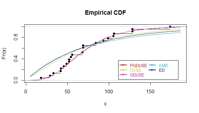
Figure 3: The empirical cumulative density functions of the models.

6 Conclusion

In this article, a new class of distribution by generalizing the DUS transformation, called the PGDUS transformation is introduced. A new lifetime distribution called the PGDUSE distribution with exponential as the baseline distribution is also proposed. The generalized form provides greater flexibility in modelling real datasets. Different statistical properties such as moments, moment generating function, characteristic function, quantile function, cumulant generating function, order statistic and entropy are derived. The parameter estimation has been done through the method of maximum likelihood. Lastly, a real data analysis is performed to show that the proposed generalization can be used effectively to provide better fits.

References

References

• [1] Cordeiro, G. M., and de Castro M.(2011), A new family of generalized distributions, Journal of Statistical Computation and Simulation, 81(7), 883-898.
• [2] Cordeiro, G. M., Ortega, E. M. M., and da Cunha, D. C. C.(2013), The exponentiated generalized class of distributions, Journal of Data Science,11,1-27.
• [3] Deepthi, K. S. and Chacko, V. M.(2020), An upside-down bathtub-shaped failure rate model using a DUS transformation of Lomax distribution, Lirong Cui, Ilia Frenkel, Anatoly Lisnianski (Eds), Stochastic Models in Reliability Engineering, chapter 6, 81-100. Taylor & Francis Group, Boca Raton, CRC Press.
• [4] Gauthami, P. and Chacko, V. M. (2021), DUS transformation of Inverse Weibull distribution: An upside-down failure rate rate model, Reliaility: Theory and Applications,Vol 16, No 2(62),58-71.
• [5] Gupta, R. C., Gupta, R. D., and Gupta, P. L.(1998), A method of proposing new distribution and its application to bladder cancer patients data, Communications in Statistics - Theory and Methods, 27, 887-904.
• [6] Kavya, P., Manoharan, M.(2020), On a Generalized lifetime model using DUS transformation, Joshua, V., Varadhan, S., Vishnevsky, V. (Eds), Applied Probability and Stochastic Processes, 281-291. Infosys Science Foundation Series, Springer, Singapore.
• [7] Kumar, D., Singh, U., and Singh, S. K.(2015), A method of proposing new distribution and its application to bladder cancer patients data, Journal of Statistics Applications and Probability Letters, 2(3), 235-245.
• [8] Kumar, D., Singh, U., and Singh, S. K.(2015), A new distribution using sine function - its application to bladder cancer patients data, Journal of Statistics Applications and Probability Letters, 5;4(3), 417-427.
• [9] Lawless, J. F., (1982), Statistical models and methods for lifetime data. John Wiley and Sons, New York.
• [10] Maurya, S. K., Kaushik, A., Singh, S. K., and Singh, U.(2016), A new class of exponential transformed Lindley distribution and its application to Yarn data, International Journal of Statistics and Economics, 18(2).
• [11] Nadarajah, S., Kotz, S.,(2006), The exponentiated type distributions,Acta Applicandae Mathematica,92(2), 97-111.
• [12] Tripathi, A., Singh, U. and Singh, S. K.(2019), Inferences for the DUS-Exponential Distribution Based on upper record values, Annals of Data Science, 1-17.