The UHECR dipole and quadrupole in the latest data from the original Auger and TA surface detectors

Abstract

The sources of ultra-high-energy cosmic rays are still unknown, but assuming standard physics, they are expected to lie within a few hundred megaparsecs from us. Indeed, over cosmological distances cosmic rays lose energy to interactions with background photons, at a rate depending on their mass number and energy and properties of photonuclear interactions and photon backgrounds. The universe is not homogeneous at such scales, hence the distribution of the arrival directions of cosmic rays is expected to reflect the inhomogeneities in the distribution of galaxies; the shorter the energy loss lengths, the stronger the expected anisotropies. Galactic and intergalactic magnetic fields can blur and distort the picture, but the magnitudes of the largest-scale anisotropies, namely the dipole and quadrupole moments, are the most robust to their effects. Measuring them with no bias regardless of any higher-order multipoles is not possible except with full-sky coverage. In this work, we achieve this in three energy ranges (approximately $8$–$16~{}\mathrm{EeV}$, $16$–$32~{}\mathrm{EeV}$, and $32$–$\infty~{}\mathrm{EeV}$) by combining surface-detector data collected at the Pierre Auger Observatory until 2020 and at the Telescope Array (TA) until 2019, before the completion of the upgrades of the arrays with new scintillator detectors. We find that the full-sky coverage achieved by combining Auger and TA data reduces the uncertainties on the north-south components of the dipole and quadrupole in half compared to Auger-only results.

1 Introduction

While on general grounds the anisotropies of cosmic rays (CR) at highest energies are expected to give a key to understanding of their sources, in practice the deflections of cosmic rays in (highly uncertain) magnetic fields make this task extremely difficult. Even though the angular resolution in the reconstruction of CR arrival directions is good (${\sim}1^{\circ}$), no anisotropies have been discovered at small angular scales of order a few degrees, likely due to a washing effect of the magnetic deflections.

Even when individual sources are not resolved, at large angular scales the anisotropies are expected to arise from a non-homogeneous source distribution in the Universe at distances of 50–100 Mpc. The effect of magnetic deflections at these angular scales, particularly for the dipole and quadrupole harmonics, may not be dominant. The non-zero dipole anisotropy in the CR distribution, with an amplitude of $6.5\%$ in the equatorial plane, has indeed been discovered by the Pierre Auger Observatory (hereafter Auger) [1] at energies $E>8$ EeV. The equatorial dipole has also been measured by the Telescope Array (TA) [2], with the result in agreement with that of Auger but not significant alone due to small statistics.

Both Auger and TA observatories have incomplete sky coverage, which makes the unambiguous determination of all multipole components impossible. To achieve the full-sky coverage, they have to be combined together. However, this cannot be trivially done by simply combining the events detected by the two observatories with their nominal energy estimates, as they both have potentially different systematic uncertainties in the energy determination, and these differences may affect the sky distribution of events in a given energy range in the combined data set. The energy scales have to be cross-calibrated before combining the data. This can be done from the data themselves without any extra assumptions on the nature of the energy determination systematics [3] by comparing the data of the two observatories in the equatorial band where their exposures overlap.

The purpose of this study is to cross-calibrate energy scales of the Auger and TA observatories in the energy range $E\gtrsim 10$ EeV and to determine in an assumption-free way the dipole and quadrupole components of the UHECR flux in this energy range. This study is a development of the previous analyses [3, 4, 5] in the following three respects: (i) we use the updated data sets, (ii) we cross-calibrate the energy scales in three energy bins relaxing the assumption that the difference in energy scales is energy-independent and (iii) we carefully trace all sources of uncertainties and propagate them into the final result.

2 The datasets

The Pierre Auger Observatory [6] is a hybrid detector of UHECRs located in the Southern hemisphere in Argentina at a latitude of $-35.2^{\circ}$. It consists of a surface array of 1660 water-Cherenkov detectors covering an area of approximately 3000 km², overlooked by the fluorescence detector composed of 27 fluorescence telescopes. The detector is taking data since January 2004. In this work, we use the dataset described in Ref. [7], consisting of events detected by the surface detector (SD) array from 2004 Jan 01 to 2020 Dec 31. Its geometric exposure is $110\,000~{}\mathrm{km}^{2}~{}\mathrm{yr}~{}\mathrm{sr}$. In order to correct for the effects of the finite energy resolution, which in the case of a decreasing energy spectrum tend to make the raw measured spectrum higher than the actual one, we divide the geometric exposures by the unfolding correction factors reported in Ref. [8], which in the energy range used in this work, increase from 0.977 in the energy bin $18.9\leq\log_{10}(E/\mathrm{eV})<19.0$ to 1.002 in the bin $19.6\leq\log_{10}(E/\mathrm{eV})<19.7$ then decrease again to 0.964 in the bins $\log_{10}(E/\mathrm{eV})\geq 19.8$. The effects of the tilt of the SD array and of the non-uniformity of its aperture in sidereal time were found to be minor in Ref. [1] (of the order of $1/4$ and $1/20$ of the statistical uncertainties, respectively) and are neglected in this work.

The Telescope Array [9] is a hybrid detector of UHECRs located in the Northern hemisphere in Utah, USA at a latitude of $39.3^{\circ}$. It is taking data since May 2008. The surface detector of TA consists of 507 plastic scintillator detectors covering an area of about 700 km². The fluorescence detector of TA is composed of 38 fluorescence telescopes arranged in 3 towers overlooking the surface detector area. In this work, we use the events with the zenith angles $\theta<55^{\circ}$ detected by the TA SD array from 2008 May 11 to 2019 May 10 with the selection criteria as described in [3]. The effective exposure, accounting for the effects of the energy resolution, in the energy range used in this work depends non-monotonically on energy, with a minimum value of $13\,200~{}\mathrm{km}^{2}~{}\mathrm{yr}~{}\mathrm{sr}$ in the energy bin $19.7\leq\log_{10}(E/\mathrm{eV})<19.8$, a maximum of $15\,400~{}\mathrm{km}^{2}~{}\mathrm{yr}~{}\mathrm{sr}$ in $20.0\leq\log_{10}(E/\mathrm{eV})<20.1$, and a value of $15\,100~{}\mathrm{km}^{2}~{}\mathrm{yr}~{}\mathrm{sr}$ in the bins $\log_{10}(E/\mathrm{eV})\geq 20.2$.

We assume that the effective exposure of each detector array factorizes into an effective area $\mathcal{E}$ which depends on the energy $E$ but not on the arrival direction, and a geometric exposure $\omega_{\text{geom}}$ which only depends on the declination as described in Ref. [10]. In the case of Auger, we consider two different effective areas for vertical ($\theta<60^{\circ}$) and inclined ($\theta\geq 60^{\circ}$) events due to the different reconstruction techniques used for these two zenith angle ranges.

Figure 1: The combined Auger + TA effective exposure in the first energy bin, see Sect. 3. The yellow band on the left panel indicates the range of declinations visible to both observatories used for the cross-calibration of energy scales.

As an example, the combined exposure averaged over the lowest of the three energy bins in which we search for anisotropies (see Sect. 3) is shown in Fig. 1.

3 The cross-calibration of energy scale

As already mentioned, when combining data from different detectors to infer the large-scale anisotropy, it is important to ensure that the energy thresholds used for them match, otherwise spurious detections of the north-south anisotropy may arise. To eliminate this problem, we calibrate the Auger and TA energy scales to each other using the events detected in the equatorial region of the sky where both observatories have exposure (see Fig. 1). The idea behind the cross-calibration procedure is that the true UHECR flux integrated over the common band as a function of energy, $\phi^{\rm true}(E)$, can be estimated in each of the two observatories independently. When the energy scales match, these two estimates must agree at all energies. Note that this procedure does not allow one to determine the true energy scale, only to eliminate a possible mismatch in scales between the two observatories. This is sufficient, however, for the purpose of the present analysis.

To estimate the flux we use the unbiased estimator introduced in [11], which is essentially the sum over events in the band weighted with the inverse exposure $\omega_{a}$ of each observatory $a=(\text{Auger, TA})$. In the energy bin $j$, defined in terms of the nominal energy of the corresponding observatory, the flux estimate is $\phi^{\text{est.}}_{aj}=\sum_{k}1/\omega_{a}(\mathbf{n}_{k})$, where $\mathbf{n}_{k}$ is the arrival direction of a given event and the sum runs over the events $k$ with energies $E_{ak}\in[E_{aj},E_{aj+1})$ and arrival directions in the common band $\delta_{k}\in(\delta_{\min},\delta_{\max})$. It can be shown that, provided the exposure does not vanish anywhere in the band and regardless of the variations of the flux density $J(E,\mathbf{n})$ over the sky, the quantity $\phi^{\text{est.}}_{aj}$ is an unbiased estimator of $\phi^{\text{true}}_{j}=\int_{E_{aj}}^{E_{aj+1}}\int_{\delta_{\min}}^{\delta_{\max}}J(E,\mathbf{n})\,\mathrm{d}E\,\mathrm{d}\Omega$. The latter is by definition a detector-independent quantity, and hence, in the absence of energy scale differences, the two estimators $\phi^{\text{est.}}_{{\rm Auger,}j}$ and $\phi^{\text{est.}}_{{\rm TA,}j}$ must agree within statistical uncertainties in all energy bins. The cross-calibration consists in determining the energy conversion function between the two observatories such that this requirement is satisfied. Unlike in Refs. [4, 5], where the cross-calibration was applied to energy thresholds — which is equivalent to assuming a constant energy rescaling factor — in this work we assume a functional form for the $E_{\text{TA}}\leftrightarrow E_{\text{Auger}}$ conversion with free parameters which we fit to satisfy the flux matching conditions in the common band.

The fiducial boundaries of the common band are chosen as follows. The intersection of the Auger and TA fields of view is $(-15.7^{\circ},+44.8^{\circ})$, but in the areas close to the edge $1/\omega_{i}$ becomes very large, which would result in increased statistical uncertainties if the entire intersection was used. Instead, we choose a fiducial band $(\delta_{\min}=-11^{\circ},\delta_{\max}=+43^{\circ})$, which are the values that minimize the expected total statistical uncertainties rounded to the nearest degree.

We bin the events in logarithmic nominal energy bins defined as $\log_{10}(E_{\text{Auger},j}/\mathrm{eV})=18.9+0.1j$ and $\log_{10}(E_{\text{TA},j}/\mathrm{eV})=19.0+0.1j$, for $j=0$, $1$, . . . The last non-empty bin is $[20.1,20.2)$ for Auger and $[20.2,20.3)$ for TA. We then compute the corresponding statistical uncertainties of the flux estimators as $\sigma_{aj}=\sqrt{\sum_{k}1/\omega_{a}(E_{k},\mathbf{n}_{k})^{2}}$, where the sum runs over the same events as above.

We assume a power law for the energy conversion in the range $E_{\text{TA}}\geq 10~{}\mathrm{EeV}$ characterized by two parameters ${\boldsymbol{\theta}}_{E}=(\alpha,\beta)$:

$$E_{\text{Auger}} =E_{0}e^{\alpha}\left(E_{\text{TA}}/E_{0}\right)^{\beta},$$

$$E_{\text{TA}} =E_{0}e^{-\alpha/\beta}\left(E_{\text{Auger}}/E_{0}\right)^{1/\beta}$$ (1)

with $E_{0}=10~{}\mathrm{EeV}$. The goal of the cross-calibration is to determine the parameters $\alpha$ and $\beta$. If we binned the events in corrected energies, events would move from one bin to another when the parameters are changed, producing discontinuities in the flux estimator. To avoid this technical problem, we fit both Auger and TA data to a model spectrum in the band while keeping both sets of nominal energy bins fixed. For the model spectrum we use the twice-broken power law ($\propto E^{-\gamma}$) with normalization $\mathcal{J}_{0}$, break energies ${E_{\mathrm{AB}}}$ and ${E_{\mathrm{BC}}}$ and spectral indices ${\gamma_{\mathrm{A}}}$, ${\gamma_{\mathrm{B}}}$ and ${\gamma_{\mathrm{C}}}$, for a total of six additional parameters ${\boldsymbol{\theta}}_{J}$. For each set of resulting 8 parameters, we compute the model predictions $\phi^{\text{pred}}_{j}({\boldsymbol{\theta}}_{J},{\boldsymbol{\theta}}_{E})=\int_{E_{j}}^{E_{j+1}}\mathcal{J}_{\text{band}}(E;{\boldsymbol{\theta}}_{J})\operatorname{d}\!{E}$ where $E$ is some (arbitrarily chosen) energy scale and the bin boundaries $E_{i}$ are obtained by converting the bins of the corresponding observatory into that scale. Finally, we compute $\chi^{2}$ according to a log-normal distribution,

$$\chi^{2}=\sum_{aj}\frac{\bigl{(}\ln\phi_{aj}^{\text{est.}}-\ln\phi^{\text{pred.}}_{aj}({\boldsymbol{\theta}}_{J},{\boldsymbol{\theta}}_{E})\bigr{)}^{2}}{\bigl{(}\sigma_{aj}\big{/}\phi^{\text{est.}}_{aj}\bigr{)}^{2}},$$ (2)

which we found to adequately describe the probability distribution of the flux estimator in simulations provided there are ${\gtrsim}10$ events in the fiducial band in each energy bin, which we achieve by combining together the last energy bins of each dataset until this condition is achieved (for Auger, 19 events with $\log_{10}(E/\mathrm{eV})\geq 19.9$; for TA, 11 events with $\log_{10}(E/\mathrm{eV})\geq 20.0$, remaining with 11 bins for both Auger and TA).

			$\frac{\mathcal{J}_{0}}{\mathrm{eV}^{-1}~{}\mathrm{km}^{-2}~{}\mathrm{yr}^{-1}}$	${\gamma_{\mathrm{A}}}$	$\frac{{E_{\mathrm{AB}}}}{\mathrm{EeV}}$	${\gamma_{\mathrm{B}}}$	$\frac{{E_{\mathrm{BC}}}}{\mathrm{EeV}}$	${\gamma_{\mathrm{C}}}$
$\alpha=-0.154\pm 0.013$		Auger scale	$2.65\times 10^{-19}$	2.53	11.7	2.92	49.6	5.66
$\beta=\phantom{+}0.937\pm 0.017$		TA scale	$3.14\times 10^{-19}$	2.43	13.9	2.80	65.1	5.37
$\rho_{\alpha\beta}=-0.177$			$\chi^{2}/n_{\text{dof}}=15.6/14$ ($p=0.34$)

Table 1: Best-fit parameter values from the spectrum fit used for the cross-calibration procedure.

The resulting best fit is shown in Table 1. If the exponent $\beta$ is fixed to $1$ as corresponds to a constant rescaling factor between Auger and TA energies, the best fit becomes $\alpha=-0.163\pm 0.012$ with a $\chi^{2}/n$ of $29.1/13$. The energy-dependent rescaling of Table 1 is thus favored over a constant one at the $3.7\sigma$ level. The possible origins of such an energy-dependence are currently being investigated by the two collaborations [13].

Based on the cross-calibration results, the following energy bin boundaries have been chosen for the calculation of the dipole and quadrupole components:

Auger scale	$8.57\pm 0.11~{}\mathrm{EeV}$	$16~{}\mathrm{EeV}$	$32~{}\mathrm{EeV}$
TA scale	$10~{}\mathrm{EeV}$	$19.47\pm 0.32~{}\mathrm{EeV}$	$40.8\pm 1.1~{}\mathrm{EeV}$

The lowest energy of 10 EeV (TA) is fixed by the availability of the TA events, while the other two boundaries 16 EeV (Auger) and 32 EeV (Auger) are chosen so as to match the previous Auger dipole analysis. The exposures in these three bins, appropriately corrected for a slight energy dependence of exposure in each observatory, are $(87\,400+24\,600)~{}\mathrm{km}^{2}~{}\mathrm{yr}~{}\mathrm{sr}$, $(87\,200+24\,600)~{}\mathrm{km}^{2}~{}\mathrm{yr}~{}\mathrm{sr}$ and $(86\,600+24\,400)~{}\mathrm{km}^{2}~{}\mathrm{yr}~{}\mathrm{sr}$ for Auger vertical + inclined and $14\,200~{}\mathrm{km}^{2}~{}\mathrm{yr}~{}\mathrm{sr}$, $14\,000~{}\mathrm{km}^{2}~{}\mathrm{yr}~{}\mathrm{sr}$ and $13\,700~{}\mathrm{km}^{2}~{}\mathrm{yr}~{}\mathrm{sr}$ for TA.

The exposures of the two detectors are only known with an uncertainty of approximately $\pm 3\%$ each. An over- or under-estimate of the TA-to-Auger exposure ratio by $\pm 4.2\%$ would result in an over- or under-estimate of the parameter $\alpha$ by $0.023$, i.e. of $E_{\text{Auger}}(E_{\text{TA}}=10~{}\mathrm{EeV})$ by $0.20~{}\mathrm{EeV}$, as well as of $\beta$ by $\mp 0.06$, meaning the relative uncertainty shrinks at higher energies. On the other hand, the effect of such an uncertainty on the final anisotropy results would almost completely cancel out those of the uncertainty in the exposure ratio itself. For this reason, we neglect this source of uncertainty in the following.

3.1 Propagation of the statistical uncertainty on the calibration fit

The uncertainty on the correspondence between energy thresholds causes as an “effective” uncertainty on the exposure ratio. If we overestimate e.g. the Auger threshold corresponding to a given TA threshold, we underestimate the flux in the Auger field of view. The effect on large-scale anisotropy searches can be approximated to that of overestimating its exposure, provided the anisotropies themselves do not appreciably change with energy over such a range. To quantify this uncertainty, we propagate the statistical uncertainties of the fit on $\alpha$ and $\beta$ (Table 1) to the quantity

$$\ln\left(\frac{\phi^{\text{pred}}_{\text{TA},j^{\prime}}({\boldsymbol{\theta}}_{J},\alpha_{\text{best}},\beta_{\text{best}})}{\phi^{\text{pred}}_{\text{TA},j^{\prime}}({\boldsymbol{\theta}}_{J},\alpha,\beta)}\frac{\phi^{\text{pred}}_{\text{Auger},j^{\prime}}({\boldsymbol{\theta}}_{J},\alpha,\beta)}{\phi^{\text{pred}}_{\text{Auger},j^{\prime}}({\boldsymbol{\theta}}_{J},\alpha_{\text{best}},\beta_{\text{best}})}\right)$$ (3)

where $\phi^{\text{pred}}_{ij^{\prime}}$ is computed as above, but over the “wide” energy bins $j^{\prime}$ we are going to use for anisotropy searches, not the “narrow” energy bins $j$ used for the cross-calibration — in other words, how much we would overestimate the TA-to-Auger flux ratio if the true conversion parameters were $(\alpha,\beta)$ but we assumed they were $(\alpha_{\text{best}},\beta_{\text{best}})$. The result is $\pm 2.5\%$, $\pm 2.5\%$ and $\pm 6.5\%$ in the first, second and third energy bin, respectively. It can be noted that these values are roughly of the order of $(\gamma-1)$ times the relative uncertainties on the energy thresholds, as they would be in the case of a single threshold for an integral flux $\int_{E}^{+\infty}\mathcal{J}_{\text{band}}(E)\operatorname{d}\!{E}\propto E^{-(\gamma-1)}$.

4 Results on large-scale anisotropies

The UHECR flux $\Phi(\mathbf{n})$ can be represented as a sum of spherical harmonics $Y_{lm}$,

$$\Phi(\mathbf{n}) =\sum_{\ell=0}^{+\infty}\sum_{m=-\ell}^{+\ell}a_{\ell m}Y_{\ell m}(\mathbf{n}), a_{\ell m} =\int_{4\pi}Y_{\ell m}(\mathbf{n})\Phi(\mathbf{n})\operatorname{d}\!\Omega.$$ (4)

The coefficients $a_{\ell m}$ represent anisotropies on scales $\mathcal{O}(180^{\circ}/\ell)$. The contribution of the two lowest non-trivial harmonics $l=1,2$, the dipole and quadrupole, can be rewritten in terms of a dipole vector $\mathbf{d}$ and the symmetric traceless quadrupole tensor $Q_{ij}$ as follows,

$$\Phi(\mathbf{n})=\Phi_{0}\left(1+\mathbf{d}\cdot\mathbf{n}+\tfrac{1}{2}\mathbf{n}\cdot\mathsf{Q}\mathbf{n}+\cdots\right)$$ (5)

where $\Phi_{0}=\sqrt{4\pi}\,a_{00}$, $d_{x}=\sqrt{3}a_{11}/a_{00}$, $d_{y}=\sqrt{3}a_{1-1}/a_{00}$, $d_{z}=\sqrt{3}a_{10}/a_{00}$, $Q_{xx}-Q_{yy}=2\sqrt{15}a_{22}/a_{00}$, $Q_{xz}=\sqrt{15}a_{21}/a_{00}$, $Q_{yz}=\sqrt{15}a_{2-1}/a_{00}$, $Q_{zz}=2\sqrt{5}a_{20}/a_{00}$, $Q_{xy}=\sqrt{15}a_{2-2}/a_{00}$ and the other components of $Q_{ij}$ can be computed from its symmetry and zero trace condition.

Using a full-sky dataset with the combined exposure $\omega(\mathbf{n})$ non-zero everywhere, each $a_{\ell m}$ can be estimated independently as $\sum_{k}Y_{\ell m}(\mathbf{n}_{k})/\omega(\mathbf{n}_{k})$. We estimate the statistic uncertainties and the correlations between them as $\sigma_{\ell m}\sigma_{\ell^{\prime}m^{\prime}}\rho_{\ell m,\ell^{\prime}m^{\prime}}=\sum_{k}Y_{\ell m}(\mathbf{n}_{k})Y_{\ell^{\prime}m^{\prime}}(\mathbf{n}_{k})/\omega(\mathbf{n}_{k})^{2}$. As for the uncertainties due to the energy cross-calibration, we compute them by computing $a_{\ell m}^{\pm}$ assuming the exposure $\omega^{\pm}=\omega_{\text{Auger}}+e^{\pm k}\omega_{\text{TA}}$ where $k$ is the “effective” exposure ratio uncertainty described in subsection 3.1, and taking $\sigma_{\text{syst}}(d_{z})=\frac{1}{2}(d_{z}^{+}-d_{z}^{-})$, $\sigma_{\text{syst}}(Q_{zz})=\frac{1}{2}(Q_{zz}^{+}-Q_{zz}^{-})$, and similarly for other components. The rotationally invariant quantities $C_{1}=\tfrac{4\pi}{9}\left|\mathbf{d}\right|$ and $C_{2}=\tfrac{2\pi}{75}\sum_{ij}Q_{ij}^{2}$ (normalized to $C_{0}=4\pi$ i.e. to $\Phi_{0}=1$) can also be computed as $C_{\ell}=\frac{1}{2\ell+1}\sum_{m=-\ell}^{+\ell}a_{\ell m}^{2}$.

energies (Auger)	$[8.57~{}\mathrm{EeV},16~{}\mathrm{EeV})$	$[16~{}\mathrm{EeV},32~{}\mathrm{EeV})$	$[32~{}\mathrm{EeV},+\infty)$
energies (TA)	$[10~{}\mathrm{EeV},19.47~{}\mathrm{EeV})$	$[19.47~{}\mathrm{EeV},40.8~{}\mathrm{EeV})$	$[40.8~{}\mathrm{EeV},+\infty)$
$d_{x}~{}[\%]$	$-0.7\pm 1.1\pm 0.0$	$+1.6\pm 2.0\pm 0.0$	$-5.3\pm 3.9\pm 0.1$
$d_{y}~{}[\%]$	$+4.8\pm 1.1\pm 0.0$	$+3.9\pm 1.9\pm 0.1$	$+9.7\pm 3.7\pm 0.0$
$d_{z}~{}[\%]$	$-3.3\pm 1.4\pm 1.3$	$-6.0\pm 2.4\pm 1.3$	$+3.4\pm 4.7\pm 3.6$
$Q_{xx}-Q_{yy}~{}[\%]$	$-5.1\pm 4.8\pm 0.0$	$+13.6\pm 8.3\pm 0.0\phantom{0}$	$+43\pm 16\pm 0\phantom{0}$
$Q_{xz}~{}[\%]$	$-3.9\pm 2.9\pm 0.1$	$+5.4\pm 5.1\pm 0.0$	$+5\pm 11\pm 0$
$Q_{yz}~{}[\%]$	$-4.9\pm 2.9\pm 0.0$	$-9.6\pm 5.0\pm 0.1$	$+11.9\pm 9.8\pm 0.2\phantom{0}$
$Q_{zz}~{}[\%]$	$+0.5\pm 3.3\pm 1.7$	$+5.2\pm 5.8\pm 1.7$	$+20\pm 11\pm 5\phantom{0}$
$Q_{xy}~{}[\%]$	$+2.2\pm 2.4\pm 0.0$	$+0.2\pm 4.2\pm 0.1$	$+4.5\pm 8.1\pm 0.1$
$C_{1}~{}[10^{-3}]$	$4.8\pm 2.0\pm 1.2$	$7.6\pm 4.6\pm 2.2$	$19\pm 12\pm 4$
$C_{2}~{}[10^{-3}]$	$0.85\pm 0.66\pm 0.02$	$3.1\pm 2.2\pm 0.2$	$15.5\pm 8.9\pm 2.4$

Table 2: The dipole and quadrupole moments estimated from our data. The first uncertainty is statistical, the second is due to that on the energy cross-calibration. The statistical uncertainties are uncorrelated ($-0.1<\rho<0.1$) except $\rho(d_{x},Q_{xz})=\rho(d_{y},Q_{yz})=0.45$ and $\rho(d_{z},Q_{zz})=0.53$.

The results in the three energy bins defined above are shown in Table 2.

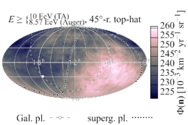
Figure 2: Left: Spherical harmonic expansion of the flux inferred from our data up to $\ell=2$ (dipole and quadrupole) in the three energy bins. Right: Measured flux averaged over $45^{\circ}$-radius top-hat windows.

The spherical harmonic expansion of the UHECR flux in these bins, truncated at $\ell\leq 2$, is shown in Figure 2 in comparison with the flux estimate from the combined data in the corresponding bin, smoothed with the window size of $45^{\circ}$.

5 Discussion

Using full-sky data, we have estimated the dipole and quadrupole moments of the UHECR flux distribution without any assumptions about higher-order multipoles. The results are compatible with Auger-only ones assuming $\ell_{\max}=2$ [7], but with uncertainties on $d_{z}$ and $Q_{zz}$ about twice as small, as well as slightly smaller uncertainties on the other dipole and quadrupole components. None of the moments shown in Table 2 are significant with $>3\sigma$ pre-trial significance, except the dipole along the $y$ axis in the lowest energy bin already reported in Ref. [1].

The Pierre Auger Collaboration

P. Abreu⁷², M. Aglietta^54,52, J.M. Albury¹³, I. Allekotte¹, A. Almela^8,12, J. Alvarez-Muñiz⁷⁹, R. Alves Batista⁸⁰, G.A. Anastasi^63,52, L. Anchordoqui⁸⁷, B. Andrada⁸, S. Andringa⁷², C. Aramo⁵⁰, P.R. Araújo Ferreira⁴², J. C. Arteaga Velázquez⁶⁷, H. Asorey⁸, P. Assis⁷², G. Avila¹¹, A.M. Badescu⁷⁵, A. Bakalova³², A. Balaceanu⁷³, F. Barbato^45,46, R.J. Barreira Luz⁷², K.H. Becker³⁸, J.A. Bellido^13,69, C. Berat³⁶, M.E. Bertaina^63,52, X. Bertou¹, P.L. Biermann^b, V. Binet⁶, K. Bismark^39,8, T. Bister⁴², J. Biteau³⁷, J. Blazek³², C. Bleve³⁶, M. Boháčová³², D. Boncioli^57,46, C. Bonifazi^9,26, L. Bonneau Arbeletche²¹, N. Borodai⁷⁰, A.M. Botti⁸, J. Brack^d, T. Bretz⁴², P.G. Brichetto Orchera⁸, F.L. Briechle⁴², P. Buchholz⁴⁴, A. Bueno⁷⁸, S. Buitink¹⁵, M. Buscemi⁴⁷, M. Büsken^39,8, K.S. Caballero-Mora⁶⁶, L. Caccianiga^59,49, F. Canfora^80,81, I. Caracas³⁸, J.M. Carceller⁷⁸, R. Caruso^58,47, A. Castellina^54,52, F. Catalani¹⁹, G. Cataldi⁴⁸, L. Cazon⁷², M. Cerda¹⁰, J.A. Chinellato²², J. Chudoba³², L. Chytka³³, R.W. Clay¹³, A.C. Cobos Cerutti⁷, R. Colalillo^60,50, A. Coleman⁹³, M.R. Coluccia⁴⁸, R. Conceição⁷², A. Condorelli^45,46, G. Consolati^49,55, F. Contreras¹¹, F. Convenga^56,48, D. Correia dos Santos²⁸, C.E. Covault⁸⁵, S. Dasso^5,3, K. Daumiller⁴¹, B.R. Dawson¹³, J.A. Day¹³, R.M. de Almeida²⁸, J. de Jesús^8,41, S.J. de Jong^80,81, G. De Mauro^80,81, J.R.T. de Mello Neto^26,27, I. De Mitri^45,46, J. de Oliveira¹⁸, D. de Oliveira Franco²², F. de Palma^56,48, V. de Souza²⁰, E. De Vito^56,48, M. del Río¹¹, O. Deligny³⁴, L. Deval^41,8, A. di Matteo⁵², C. Dobrigkeit²², J.C. D’Olivo⁶⁸, L.M. Domingues Mendes⁷², R.C. dos Anjos²⁵, D. dos Santos²⁸, M.T. Dova⁴, J. Ebr³², R. Engel^39,41, I. Epicoco^56,48, M. Erdmann⁴², C.O. Escobar^a, A. Etchegoyen^8,12, H. Falcke^80,82,81, J. Farmer⁹², G. Farrar⁹⁰, A.C. Fauth²², N. Fazzini^a, F. Feldbusch⁴⁰, F. Fenu^54,52, B. Fick⁸⁹, J.M. Figueira⁸, A. Filipčič^77,76, T. Fitoussi⁴¹, T. Fodran⁸⁰, M.M. Freire⁶, T. Fujii^92,e, A. Fuster^8,12, C. Galea⁸⁰, C. Galelli^59,49, B. García⁷, A.L. Garcia Vegas⁴², H. Gemmeke⁴⁰, F. Gesualdi^8,41, A. Gherghel-Lascu⁷³, P.L. Ghia³⁴, U. Giaccari⁸⁰, M. Giammarchi⁴⁹, J. Glombitza⁴², F. Gobbi¹⁰, F. Gollan⁸, G. Golup¹, M. Gómez Berisso¹, P.F. Gómez Vitale¹¹, J.P. Gongora¹¹, J.M. González¹, N. González¹⁴, I. Goos^1,41, D. Góra⁷⁰, A. Gorgi^54,52, M. Gottowik³⁸, T.D. Grubb¹³, F. Guarino^60,50, G.P. Guedes²³, E. Guido^52,63, S. Hahn^41,8, P. Hamal³², M.R. Hampel⁸, P. Hansen⁴, D. Harari¹, V.M. Harvey¹³, A. Haungs⁴¹, T. Hebbeker⁴², D. Heck⁴¹, G.C. Hill¹³, C. Hojvat^a, J.R. Hörandel^80,81, P. Horvath³³, M. Hrabovský³³, T. Huege^41,15, A. Insolia^58,47, P.G. Isar⁷⁴, P. Janecek³², J.A. Johnsen⁸⁶, J. Jurysek³², A. Kääpä³⁸, K.H. Kampert³⁸, N. Karastathis⁴¹, B. Keilhauer⁴¹, J. Kemp⁴², A. Khakurdikar⁸⁰, V.V. Kizakke Covilakam^8,41, H.O. Klages⁴¹, M. Kleifges⁴⁰, J. Kleinfeller¹⁰, M. Köpke³⁹, N. Kunka⁴⁰, B.L. Lago¹⁷, R.G. Lang²⁰, N. Langner⁴², M.A. Leigui de Oliveira²⁴, V. Lenok⁴¹, A. Letessier-Selvon³⁵, I. Lhenry-Yvon³⁴, D. Lo Presti^58,47, L. Lopes⁷², R. López⁶⁴, L. Lu⁹⁴, Q. Luce³⁹, J.P. Lundquist⁷⁶, A. Machado Payeras²², G. Mancarella^56,48, D. Mandat³², B.C. Manning¹³, J. Manshanden⁴³, P. Mantsch^a, S. Marafico³⁴, A.G. Mariazzi⁴, I.C. Mariş¹⁴, G. Marsella^61,47, D. Martello^56,48, S. Martinelli^41,8, O. Martínez Bravo⁶⁴, M. Mastrodicasa^57,46, H.J. Mathes⁴¹, J. Matthews⁸⁸, G. Matthiae^62,51, E. Mayotte³⁸, P.O. Mazur^a, G. Medina-Tanco⁶⁸, D. Melo⁸, A. Menshikov⁴⁰, K.-D. Merenda⁸⁶, S. Michal³³, M.I. Micheletti⁶, L. Miramonti^59,49, S. Mollerach¹, F. Montanet³⁶, C. Morello^54,52, M. Mostafá⁹¹, A.L. Müller⁸, M.A. Muller²², K. Mulrey¹⁵, R. Mussa⁵², M. Muzio⁹⁰, W.M. Namasaka³⁸, A. Nasr-Esfahani³⁸, L. Nellen⁶⁸, M. Niculescu-Oglinzanu⁷³, M. Niechciol⁴⁴, D. Nitz⁸⁹, D. Nosek³¹, V. Novotny³¹, L. Nožka³³, A Nucita^56,48, L.A. Núñez³⁰, M. Palatka³², J. Pallotta², P. Papenbreer³⁸, G. Parente⁷⁹, A. Parra⁶⁴, J. Pawlowsky³⁸, M. Pech³², F. Pedreira⁷⁹, J. Pȩkala⁷⁰, R. Pelayo⁶⁵, J. Peña-Rodriguez³⁰, E.E. Pereira Martins^39,8, J. Perez Armand²¹, C. Pérez Bertolli^8,41, M. Perlin^8,41, L. Perrone^56,48, S. Petrera^45,46, T. Pierog⁴¹, M. Pimenta⁷², V. Pirronello^58,47, M. Platino⁸, B. Pont⁸⁰, M. Pothast^81,80, P. Privitera⁹², M. Prouza³², A. Puyleart⁸⁹, S. Querchfeld³⁸, J. Rautenberg³⁸, D. Ravignani⁸, M. Reininghaus^41,8, J. Ridky³², F. Riehn⁷², M. Risse⁴⁴, V. Rizi^57,46, W. Rodrigues de Carvalho²¹, J. Rodriguez Rojo¹¹, M.J. Roncoroni⁸, S. Rossoni⁴³, M. Roth⁴¹, E. Roulet¹, A.C. Rovero⁵, P. Ruehl⁴⁴, A. Saftoiu⁷³, F. Salamida^57,46, H. Salazar⁶⁴, G. Salina⁵¹, J.D. Sanabria Gomez³⁰, F. Sánchez⁸, E.M. Santos²¹, E. Santos³², F. Sarazin⁸⁶, R. Sarmento⁷², C. Sarmiento-Cano⁸, R. Sato¹¹, P. Savina^56,48,34,94, C.M. Schäfer⁴¹, V. Scherini^56,48, H. Schieler⁴¹, M. Schimassek^39,8, M. Schimp³⁸, F. Schlüter^41,8, D. Schmidt³⁹, O. Scholten^84,15, P. Schovánek³², F.G. Schröder^93,41, S. Schröder³⁸, J. Schulte⁴², S.J. Sciutto⁴, M. Scornavacche^8,41, A. Segreto^53,47, S. Sehgal³⁸, R.C. Shellard¹⁶, G. Sigl⁴³, G. Silli^8,41, O. Sima^73,f, R. Šmída⁹², P. Sommers⁹¹, J.F. Soriano⁸⁷, J. Souchard³⁶, R. Squartini¹⁰, M. Stadelmaier^41,8, D. Stanca⁷³, S. Stanič⁷⁶, J. Stasielak⁷⁰, P. Stassi³⁶, A. Streich^39,8, M. Suárez-Durán¹⁴, T. Sudholz¹³, T. Suomijärvi³⁷, A.D. Supanitsky⁸, Z. Szadkowski⁷¹, A. Tapia²⁹, C. Taricco^63,52, C. Timmermans^81,80, O. Tkachenko⁴¹, P. Tobiska³², C.J. Todero Peixoto¹⁹, B. Tomé⁷², Z. Torrès³⁶, A. Travaini¹⁰, P. Travnicek³², C. Trimarelli^57,46, M. Tueros⁴, R. Ulrich⁴¹, M. Unger⁴¹, L. Vaclavek³³, M. Vacula³³, J.F. Valdés Galicia⁶⁸, L. Valore^60,50, E. Varela⁶⁴, A. Vásquez-Ramírez³⁰, D. Veberič⁴¹, C. Ventura²⁷, I.D. Vergara Quispe⁴, V. Verzi⁵¹, J. Vicha³², J. Vink⁸³, S. Vorobiov⁷⁶, H. Wahlberg⁴, C. Watanabe²⁶, A.A. Watson^c, M. Weber⁴⁰, A. Weindl⁴¹, L. Wiencke⁸⁶, H. Wilczyński⁷⁰, M. Wirtz⁴², D. Wittkowski³⁸, B. Wundheiler⁸, A. Yushkov³², O. Zapparrata¹⁴, E. Zas⁷⁹, D. Zavrtanik^76,77, M. Zavrtanik^77,76, L. Zehrer⁷⁶

  $\bullet$  

¹

Centro Atómico Bariloche and Instituto Balseiro (CNEA-UNCuyo-CONICET), San Carlos de Bariloche, Argentina

²

Centro de Investigaciones en Láseres y Aplicaciones, CITEDEF and CONICET, Villa Martelli, Argentina

³

Departamento de Física and Departamento de Ciencias de la Atmósfera y los Océanos, FCEyN, Universidad de Buenos Aires and CONICET, Buenos Aires, Argentina

⁴

IFLP, Universidad Nacional de La Plata and CONICET, La Plata, Argentina

⁵

Instituto de Astronomía y Física del Espacio (IAFE, CONICET-UBA), Buenos Aires, Argentina

⁶

Instituto de Física de Rosario (IFIR) – CONICET/U.N.R. and Facultad de Ciencias Bioquímicas y Farmacéuticas U.N.R., Rosario, Argentina

⁷

Instituto de Tecnologías en Detección y Astropartículas (CNEA, CONICET, UNSAM), and Universidad Tecnológica Nacional – Facultad Regional Mendoza (CONICET/CNEA), Mendoza, Argentina

⁸

Instituto de Tecnologías en Detección y Astropartículas (CNEA, CONICET, UNSAM), Buenos Aires, Argentina

⁹

International Center of Advanced Studies and Instituto de Ciencias Físicas, ECyT-UNSAM and CONICET, Campus Miguelete – San Martín, Buenos Aires, Argentina

¹⁰

Observatorio Pierre Auger, Malargüe, Argentina

¹¹

Observatorio Pierre Auger and Comisión Nacional de Energía Atómica, Malargüe, Argentina

¹²

Universidad Tecnológica Nacional – Facultad Regional Buenos Aires, Buenos Aires, Argentina

¹³

University of Adelaide, Adelaide, S.A., Australia

¹⁴

Université Libre de Bruxelles (ULB), Brussels, Belgium

¹⁵

Vrije Universiteit Brussels, Brussels, Belgium

¹⁶

Centro Brasileiro de Pesquisas Fisicas, Rio de Janeiro, RJ, Brazil

¹⁷

Centro Federal de Educação Tecnológica Celso Suckow da Fonseca, Nova Friburgo, Brazil

¹⁸

Instituto Federal de Educação, Ciência e Tecnologia do Rio de Janeiro (IFRJ), Brazil

¹⁹

Universidade de São Paulo, Escola de Engenharia de Lorena, Lorena, SP, Brazil

²⁰

Universidade de São Paulo, Instituto de Física de São Carlos, São Carlos, SP, Brazil

²¹

Universidade de São Paulo, Instituto de Física, São Paulo, SP, Brazil

²²

Universidade Estadual de Campinas, IFGW, Campinas, SP, Brazil

²³

Universidade Estadual de Feira de Santana, Feira de Santana, Brazil

²⁴

Universidade Federal do ABC, Santo André, SP, Brazil

²⁵

Universidade Federal do Paraná, Setor Palotina, Palotina, Brazil

²⁶

Universidade Federal do Rio de Janeiro, Instituto de Física, Rio de Janeiro, RJ, Brazil

²⁷

Universidade Federal do Rio de Janeiro (UFRJ), Observatório do Valongo, Rio de Janeiro, RJ, Brazil

²⁸

Universidade Federal Fluminense, EEIMVR, Volta Redonda, RJ, Brazil

²⁹

Universidad de Medellín, Medellín, Colombia

³⁰

Universidad Industrial de Santander, Bucaramanga, Colombia

³¹

Charles University, Faculty of Mathematics and Physics, Institute of Particle and Nuclear Physics, Prague, Czech Republic

³²

Institute of Physics of the Czech Academy of Sciences, Prague, Czech Republic

³³

Palacky University, RCPTM, Olomouc, Czech Republic

³⁴

CNRS/IN2P3, IJCLab, Université Paris-Saclay, Orsay, France

³⁵

Laboratoire de Physique Nucléaire et de Hautes Energies (LPNHE), Sorbonne Université, Université de Paris, CNRS-IN2P3, Paris, France

³⁶

Univ. Grenoble Alpes, CNRS, Grenoble Institute of Engineering Univ. Grenoble Alpes, LPSC-IN2P3, 38000 Grenoble, France

³⁷

Université Paris-Saclay, CNRS/IN2P3, IJCLab, Orsay, France

³⁸

Bergische Universität Wuppertal, Department of Physics, Wuppertal, Germany

³⁹

Karlsruhe Institute of Technology (KIT), Institute for Experimental Particle Physics, Karlsruhe, Germany

⁴⁰

Karlsruhe Institute of Technology (KIT), Institut für Prozessdatenverarbeitung und Elektronik, Karlsruhe, Germany

⁴¹

Karlsruhe Institute of Technology (KIT), Institute for Astroparticle Physics, Karlsruhe, Germany

⁴²

RWTH Aachen University, III. Physikalisches Institut A, Aachen, Germany

⁴³

Universität Hamburg, II. Institut für Theoretische Physik, Hamburg, Germany

⁴⁴

Universität Siegen, Department Physik – Experimentelle Teilchenphysik, Siegen, Germany

⁴⁵

Gran Sasso Science Institute, L’Aquila, Italy

⁴⁶

INFN Laboratori Nazionali del Gran Sasso, Assergi (L’Aquila), Italy

⁴⁷

INFN, Sezione di Catania, Catania, Italy

⁴⁸

INFN, Sezione di Lecce, Lecce, Italy

⁴⁹

INFN, Sezione di Milano, Milano, Italy

⁵⁰

INFN, Sezione di Napoli, Napoli, Italy

⁵¹

INFN, Sezione di Roma “Tor Vergata”, Roma, Italy

⁵²

INFN, Sezione di Torino, Torino, Italy

⁵³

Istituto di Astrofisica Spaziale e Fisica Cosmica di Palermo (INAF), Palermo, Italy

⁵⁴

Osservatorio Astrofisico di Torino (INAF), Torino, Italy

⁵⁵

Politecnico di Milano, Dipartimento di Scienze e Tecnologie Aerospaziali , Milano, Italy

⁵⁶

Università del Salento, Dipartimento di Matematica e Fisica “E. De Giorgi”, Lecce, Italy

⁵⁷

Università dell’Aquila, Dipartimento di Scienze Fisiche e Chimiche, L’Aquila, Italy

⁵⁸

Università di Catania, Dipartimento di Fisica e Astronomia, Catania, Italy

⁵⁹

Università di Milano, Dipartimento di Fisica, Milano, Italy

⁶⁰

Università di Napoli “Federico II”, Dipartimento di Fisica “Ettore Pancini”, Napoli, Italy

⁶¹

Università di Palermo, Dipartimento di Fisica e Chimica ”E. Segrè”, Palermo, Italy

⁶²

Università di Roma “Tor Vergata”, Dipartimento di Fisica, Roma, Italy

⁶³

Università Torino, Dipartimento di Fisica, Torino, Italy

⁶⁴

Benemérita Universidad Autónoma de Puebla, Puebla, México

⁶⁵

Unidad Profesional Interdisciplinaria en Ingeniería y Tecnologías Avanzadas del Instituto Politécnico Nacional (UPIITA-IPN), México, D.F., México

⁶⁶

Universidad Autónoma de Chiapas, Tuxtla Gutiérrez, Chiapas, México

⁶⁷

Universidad Michoacana de San Nicolás de Hidalgo, Morelia, Michoacán, México

⁶⁸

Universidad Nacional Autónoma de México, México, D.F., México

⁶⁹

Universidad Nacional de San Agustin de Arequipa, Facultad de Ciencias Naturales y Formales, Arequipa, Peru

⁷⁰

Institute of Nuclear Physics PAN, Krakow, Poland

⁷¹

University of Łódź, Faculty of High-Energy Astrophysics,Łódź, Poland

⁷²

Laboratório de Instrumentação e Física Experimental de Partículas – LIP and Instituto Superior Técnico – IST, Universidade de Lisboa – UL, Lisboa, Portugal

⁷³

“Horia Hulubei” National Institute for Physics and Nuclear Engineering, Bucharest-Magurele, Romania

⁷⁴

Institute of Space Science, Bucharest-Magurele, Romania

⁷⁵

University Politehnica of Bucharest, Bucharest, Romania

⁷⁶

Center for Astrophysics and Cosmology (CAC), University of Nova Gorica, Nova Gorica, Slovenia

⁷⁷

Experimental Particle Physics Department, J. Stefan Institute, Ljubljana, Slovenia

⁷⁸

Universidad de Granada and C.A.F.P.E., Granada, Spain

⁷⁹

Instituto Galego de Física de Altas Enerxías (IGFAE), Universidade de Santiago de Compostela, Santiago de Compostela, Spain

⁸⁰

IMAPP, Radboud University Nijmegen, Nijmegen, The Netherlands

⁸¹

Nationaal Instituut voor Kernfysica en Hoge Energie Fysica (NIKHEF), Science Park, Amsterdam, The Netherlands

⁸²

Stichting Astronomisch Onderzoek in Nederland (ASTRON), Dwingeloo, The Netherlands

⁸³

Universiteit van Amsterdam, Faculty of Science, Amsterdam, The Netherlands

⁸⁴

University of Groningen, Kapteyn Astronomical Institute, Groningen, The Netherlands

⁸⁵

Case Western Reserve University, Cleveland, OH, USA

⁸⁶

Colorado School of Mines, Golden, CO, USA

⁸⁷

Department of Physics and Astronomy, Lehman College, City University of New York, Bronx, NY, USA

⁸⁸

Louisiana State University, Baton Rouge, LA, USA

⁸⁹

Michigan Technological University, Houghton, MI, USA

⁹⁰

New York University, New York, NY, USA

⁹¹

Pennsylvania State University, University Park, PA, USA

⁹²

University of Chicago, Enrico Fermi Institute, Chicago, IL, USA

⁹³

University of Delaware, Department of Physics and Astronomy, Bartol Research Institute, Newark, DE, USA

⁹⁴

University of Wisconsin-Madison, Department of Physics and WIPAC, Madison, WI, USA

—–

^a

Fermi National Accelerator Laboratory, Fermilab, Batavia, IL, USA

^b

Max-Planck-Institut für Radioastronomie, Bonn, Germany

^c

School of Physics and Astronomy, University of Leeds, Leeds, United Kingdom

^d

Colorado State University, Fort Collins, CO, USA

^e

now at Hakubi Center for Advanced Research and Graduate School of Science, Kyoto University, Kyoto, Japan

^f

also at University of Bucharest, Physics Department, Bucharest, Romania

The Telescope Array Collaboration

R.U. Abbasi^1,2, T. Abu-Zayyad^1,2, M. Allen², Y. Arai³, R. Arimura³, E. Barcikowski², J.W. Belz², D.R. Bergman², S.A. Blake², I. Buckland², R. Cady², B.G. Cheon⁴, J. Chiba⁵, M. Chikawa⁶, T. Fujii⁷, K. Fujisue⁶, K. Fujita³, R. Fujiwara³, M. Fukushima⁶, R. Fukushima³, G. Furlich², R. Gonzalez², W. Hanlon², M. Hayashi⁸, N. Hayashida⁹, K. Hibino⁹, R. Higuchi⁶, K. Honda¹⁰, D. Ikeda⁹, T. Inadomi¹¹, N. Inoue¹², T. Ishii¹⁰, H. Ito¹³, D. Ivanov², H. Iwakura¹¹, A. Iwasaki³, H.M. Jeong¹⁴, S. Jeong¹⁴, C.C.H. Jui², K. Kadota¹⁵, F. Kakimoto⁹, O. Kalashev¹⁶, K. Kasahara¹⁷, S. Kasami¹⁸, H. Kawai¹⁹, S. Kawakami³, S. Kawana¹², K. Kawata⁶, I. Kharuk¹⁶, E. Kido¹³, H.B. Kim⁴, J.H. Kim², J.H. Kim², M.H. Kim¹⁴, S.W. Kim¹⁴, Y. Kimura³, S. Kishigami³, Y. Kubota¹¹, S. Kurisu¹¹, V. Kuzmin¹⁶, M. Kuznetsov^16,20, Y.J. Kwon²¹, K.H. Lee¹⁴, B. Lubsandorzhiev¹⁶, J.P. Lundquist^2,22, K. Machida¹⁰, H. Matsumiya³, T. Matsuyama³, J.N. Matthews², R. Mayta³, M. Minamino³, K. Mukai¹⁰, I. Myers², S. Nagataki¹³, K. Nakai³, R. Nakamura¹¹, T. Nakamura²³, T. Nakamura¹¹, Y. Nakamura¹¹, A. Nakazawa¹¹, E. Nishio¹⁸, T. Nonaka⁶, H. Oda³, S. Ogio^3,24, M. Ohnishi⁶, H. Ohoka⁶, Y. Oku¹⁸, T. Okuda²⁵, Y. Omura³, M. Ono¹³, R. Onogi³, A. Oshima³, S. Ozawa²⁶, I.H. Park¹⁴, M. Potts², M.S. Pshirkov^16,27, J. Remington², D.C. Rodriguez², G.I. Rubtsov¹⁶, D. Ryu²⁸, H. Sagawa⁶, R. Sahara³, Y. Saito¹¹, N. Sakaki⁶, T. Sako⁶, N. Sakurai³, K. Sano¹¹, K. Sato³, T. Seki¹¹, K. Sekino⁶, P.D. Shah², Y. Shibasaki¹¹, F. Shibata¹⁰, N. Shibata¹⁸, T. Shibata⁶, H. Shimodaira⁶, B.K. Shin²⁸, H.S. Shin⁶, D. Shinto¹⁸, J.D. Smith², P. Sokolsky², N. Sone¹¹, B.T. Stokes², T.A. Stroman², Y. Takagi³, Y. Takahashi³, M. Takamura⁵, M. Takeda⁶, R. Takeishi⁶, A. Taketa²⁹, M. Takita⁶, Y. Tameda¹⁸, H. Tanaka³, K. Tanaka³⁰, M. Tanaka³¹, Y. Tanoue³, S.B. Thomas², G.B. Thomson², P. Tinyakov^16,20, I. Tkachev¹⁶, H. Tokuno³², T. Tomida¹¹, S. Troitsky¹⁶, R. Tsuda³, Y. Tsunesada^3,24, Y. Uchihori³³, S. Udo⁹, T. Uehama¹¹, F. Urban³⁴, T. Wong², K. Yada⁶, M. Yamamoto¹¹, K. Yamazaki⁹, J. Yang³⁵, K. Yashiro⁵, F. Yoshida¹⁸, Y. Yoshioka¹¹, Y. Zhezher^6,16, and Z. Zundel²

  $\bullet$  

¹ Department of Physics, Loyola University Chicago, Chicago, Illinois, USA
² High Energy Astrophysics Institute and Department of Physics and Astronomy, University of Utah, Salt Lake City, Utah, USA
³ Graduate School of Science, Osaka City University, Osaka, Osaka, Japan
⁴ Department of Physics and The Research Institute of Natural Science, Hanyang University, Seongdong-gu, Seoul, Korea
⁵ Department of Physics, Tokyo University of Science, Noda, Chiba, Japan
⁶ Institute for Cosmic Ray Research, University of Tokyo, Kashiwa, Chiba, Japan
⁷ The Hakubi Center for Advanced Research and Graduate School of Science, Kyoto University, Kitashirakawa-Oiwakecho, Sakyo-ku, Kyoto, Japan
⁸ Information Engineering Graduate School of Science and Technology, Shinshu University, Nagano, Nagano, Japan
⁹ Faculty of Engineering, Kanagawa University, Yokohama, Kanagawa, Japan
¹⁰ Interdisciplinary Graduate School of Medicine and Engineering, University of Yamanashi, Kofu, Yamanashi, Japan
¹¹ Academic Assembly School of Science and Technology Institute of Engineering, Shinshu University, Nagano, Nagano, Japan
¹² The Graduate School of Science and Engineering, Saitama University, Saitama, Saitama, Japan
¹³ Astrophysical Big Bang Laboratory, RIKEN, Wako, Saitama, Japan
¹⁴ Department of Physics, SungKyunKwan University, Jang-an-gu, Suwon, Korea
¹⁵ Department of Physics, Tokyo City University, Setagaya-ku, Tokyo, Japan
¹⁶ Institute for Nuclear Research of the Russian Academy of Sciences, Moscow, Russia
¹⁷ Faculty of Systems Engineering and Science, Shibaura Institute of Technology, Minato-ku, Tokyo, Japan
¹⁸ Department of Engineering Science, Faculty of Engineering, Osaka Electro-Communication University, Neyagawa-shi, Osaka, Japan
¹⁹ Department of Physics, Chiba University, Chiba, Chiba, Japan
²⁰ Service de Physique Théorique, Université Libre de Bruxelles, Brussels, Belgium
²¹ Department of Physics, Yonsei University, Seodaemun-gu, Seoul, Korea
²² Center for Astrophysics and Cosmology, University of Nova Gorica, Nova Gorica, Slovenia
²³ Faculty of Science, Kochi University, Kochi, Kochi, Japan
²⁴ Nambu Yoichiro Institute of Theoretical and Experimental Physics, Osaka City University, Osaka, Osaka, Japan
²⁵ Department of Physical Sciences, Ritsumeikan University, Kusatsu, Shiga, Japan
²⁶ Quantum ICT Advanced Development Center, National Institute for Information and Communications Technology, Koganei, Tokyo, Japan
²⁷ Sternberg Astronomical Institute, Moscow M.V. Lomonosov State University, Moscow, Russia
²⁸ Department of Physics, School of Natural Sciences, Ulsan National Institute of Science and Technology, UNIST-gil, Ulsan, Korea
²⁹ Earthquake Research Institute, University of Tokyo, Bunkyo-ku, Tokyo, Japan
³⁰ Graduate School of Information Sciences, Hiroshima City University, Hiroshima, Hiroshima, Japan
³¹ Institute of Particle and Nuclear Studies, KEK, Tsukuba, Ibaraki, Japan
³² Graduate School of Science and Engineering, Tokyo Institute of Technology, Meguro, Tokyo, Japan
³³ Department of Research Planning and Promotion, Quantum Medical Science Directorate, National Institutes for Quantum and Radiological Science and Technology, Chiba, Chiba, Japan
³⁴ CEICO, Institute of Physics, Czech Academy of Sciences, Prague, Czech Republic
³⁵ Department of Physics and Institute for the Early Universe, Ewha Womans University, Seodaaemun-gu, Seoul, Korea

References

- [1] A. Aab et al. [Pierre Auger collab.], Science 357 (2017) 1266 [1709.07321].
- [2] R.U. Abbasi et al. [Telescope Array collab.], Astrophys. J. Lett. 898 (2020) L28 [2007.00023].
- [3] A. Aab et al. [Pierre Auger and Telescope Array collabs.], Astrophys. J. 794 (2014) 172 [1409.3128].
- [4] A. di Matteo et al. [for the Pierre Auger and Telescope Array collabs.], JPS Conf. Proc. 19 (2018) 011020.
- [5] J. Biteau et al. [for the Pierre Auger and Telescope Array collabs.], EPJ Web Conf. 210 (2019) 01005 [1905.04188].
- [6] A. Aab et al. [Pierre Auger collab.], Nucl. Instrum. Meth. A 798 (2015) 172 [1502.01323].
- [7] R. Menezes [for the Pierre Auger collab.], these proceedings.
- [8] A. Aab et al. [Pierre Auger collab.], Phys. Rev. D 102 (2020) 062005 [2008.06486].
- [9] T. Abu-Zayyad et al. [Telescope Array collab.], Nucl. Instrum. Meth. A 689 (2012) 87 [1201.4964].
- [10] P. Sommers, Astropart. Phys. 14 (2001) 271 [astro-ph/0004016].
- [11] T. Abu-Zayyad et al. [for the Pierre Auger and Telescope Array collabs.], JPS Conf. Proc. 19 (2018) 011003.
- [12] T. Abu-Zayyad et al. [for the Pierre Auger and Telescope Array collabs.], EPJ Web Conf. 210 (2019) 01002 [1905.04188].
- [13] Y. Tsunesada [for the Pierre Auger and Telescope Array collabs.], these proceedings.