Similarity Contrastive Estimation for Self-Supervised Soft Contrastive Learning

Abstract

Contrastive representation learning has proven to be an effective self-supervised learning method. Most successful approaches are based on Noise Contrastive Estimation (NCE) and use different views of an instance as positives that should be contrasted with other instances, called negatives, that are considered as noise. However, several instances in a dataset are drawn from the same distribution and share underlying semantic information. A good data representation should contain relations, or semantic similarity, between the instances. Contrastive learning implicitly learns relations but considering all negatives as noise harms the quality of the learned relations. To circumvent this issue, we propose a novel formulation of contrastive learning using semantic similarity between instances called Similarity Contrastive Estimation (SCE). Our training objective is a soft contrastive learning one. Instead of hard classifying positives and negatives, we estimate from one view of a batch a continuous distribution to push or pull instances based on their semantic similarities. This target similarity distribution is sharpened to eliminate noisy relations. The model predicts for each instance, from another view, the target distribution while contrasting its positive with negatives. Experimental results show that SCE is Top-1 on the ImageNet linear evaluation protocol at 100 pretraining epochs with $72.1\%$ accuracy and is competitive with state-of-the-art algorithms by reaching $75.4\%$ for 200 epochs with multi-crop. We also show that SCE is able to generalize to several tasks. Source code is available here: https://github.com/CEA-LIST/SCE.

1 Introduction

Self-Supervised learning (SSL) is an unsupervised learning procedure in which the data provides its own supervision to learn a practical representation of the data. It has been successfully applied to various applications such as classification and object detection. A pretext task is designed on the data to pretrain the model. The pretrained model is then fine-tuned on downstream tasks and several works have shown that a self-supervised pretrained network can outperform its supervised counterpart [5, 24, 6].

Contrastive learning is a state-of-the-art self-supervised paradigm based on Noise Contrastive Estimation (NCE) [25] whose most successful applications rely on instance discrimination [26, 7]. Pairs of views from same images are generated by carefully designed data augmentations [7, 48]. Elements from the same pairs are called positives and their representations are pulled together to learn view invariant features. Other images called negatives are considered as noise and their representations are pushed away from positives. Frameworks based on contrastive learning paradigm require a procedure to sample positives and negatives to learn a good data representation. A large number of negatives is essential [49] and various strategies have been proposed to enhance the number of negatives [7, 54, 26, 32]. Sampling hard negatives [32, 44, 53, 30, 19] improve the representations but can be harmful if they are semantically false negatives which is known as the ”class collision problem” [4, 52, 13].

Other approaches that learn from positive views without negatives have been proposed by predicting pseudo-classes of different views [5, 6], minimizing the feature distance of positives [24, 11] or matching the similarity distribution between views and other instances [60]. These methods free the mentioned problem of sampling hard negatives.

Based on the weakness of contrastive learning using negatives, we introduce a self-supervised soft contrastive learning approach called Similarity Contrastive Estimation (SCE), that contrasts positive pairs with other instances and leverages the push of negatives using the inter-instance similarities. Our method computes relations defined as a sharpened similarity distribution between augmented views of a batch. Each view from the batch is paired with a differently augmented query. Our objective function will maintain for each query the relations and contrast its positive with other images. A memory buffer is maintained to produce a meaningful distribution. Experiments on several datasets show that our approach outperforms our contrastive and relational baselines MoCov2 [10] and ReSSL [60].

Our contributions can be summarized as follows:

• We propose a self-supervised soft contrastive learning approach called Similarity Contrastive Estimation (SCE) that contrasts pairs of augmented images with other instances and maintains relations among instances.

• We demonstrate that our framework SCE outperforms on several benchmarks its baselines MoCov2 [10] and ReSSL [60] for a shared architecture and can further be improved using more recent architectures with a larger batch size and a predictor.

• We show that our proposed SCE is competitive with the state of the art on the ImageNet linear evaluation protocol and generalizes to several downstream tasks.

2 Related Work

Self-Supervised Learning. In early works, different pretext tasks to perform Self-Supervised Learning have been proposed to learn a good data representation such as: instance discrimination [18], patch localization [17], colorization [58], jigsaw puzzle [41], counting [42], angle rotation prediction [23].

Contrastive Learning. Contrastive learning is a learning paradigm [49, 54, 29, 47, 26, 7, 39, 48, 5, 24] that outperformed previously mentioned pretext tasks. Most successful methods rely on instance discrimination with a positive pair of views from the same image contrasted with all other instances called negatives. Retrieving lots of negatives is necessary for contrastive learning [49] and various strategies have been proposed. MoCo (v2) [26, 10] uses a small batch size and keeps a high number of negatives by maintaining a memory buffer of representations via a momentum encoder. Alternatively, SimCLR [7, 8] and MoCov3 [12] use a large batch size without a memory buffer, and without a momentum encoder for SimCLR.

Sampler for Contrastive Learning. All negatives are not equal [4] and hard negatives, negatives difficult to distinguish with positives, are the most important to sample to improve contrastive learning. However, they are potentially harmful to the training because of the “class collision” problem [4, 52, 13]. Several samplers have been proposed to alleviate this problem such as using the nearest neighbor as positive for NNCLR [19]. Truncated-triplet [50] optimizes a triplet loss using the k-th similar element as negative that showed significant improvement. It is also possible to generate views by adversarial learning as AdCo [30] showed.

Contrastive Learning without negatives. Various siamese frameworks perform contrastive learning without the use of negatives to avoid the class collision problem. BYOL [24] trains an online encoder to predict the output of a momentum updated target encoder. SwAV [5] enforces consistency between online cluster assignments from learned prototypes. DINO [6] proposes a self-distillation paradigm to match distribution on pseudo class from an online encoder to a momentum target encoder. Barlow-Twins [57] aligns the cross-correlation matrix between two paired outputs to the identity matrix that VICReg [2] stabilizes by adding an intra-batch decorrelation loss function.

Regularized Contrastive Learning. Several works regularize contrastive learning by optimizing a contrastive objective along with an objective that considers the similarities among instances. CO2 [52] adds a consistency regularization term that matches the distribution of similarity for a query and its positive. PCL [35] and WCL [59] combines unsupervised clustering with contrastive learning to tighten representations of similar instances.

Relational Learning. Contrastive learning implicitly learns relations among instances by optimizing alignment and matching a prior distribution [51, 9]. ReSSL [60] introduces an explicit relational learning objective by maintaining consistency of pairwise similarities between strong and weak augmented views. The pairs of views are not directly aligned which harms the discriminative performance.

In our work, we optimize a contrastive learning objective using negatives that alleviate class collision by pulling related instances. We do not use a regularization term but directly optimize a soft contrastive learning objective that leverages the contrastive and relational aspects.

3 Methodology

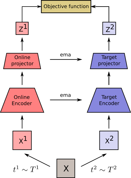
(a) Siamese pipeline

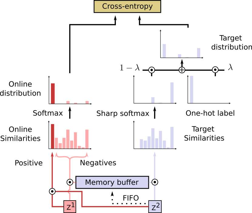
(b) SCE objective function

Figure 1: SCE follows a siamese pipeline illustrated in Fig. 1(a). A batch $\mathbf{x}$ of images is augmented with two different data augmentation distributions $T^{1}$ and $T^{2}$ to form $\mathbf{x^{1}}=t^{1}(\mathbf{x})$ and $\mathbf{x^{2}}=t^{2}(\mathbf{x})$ with $t^{1}\sim T^{1}$ and $t^{2}\sim T^{2}$. The representation $\mathbf{z^{1}}$ is computed through an online encoder $f_{s}$ and projector $g_{s}$ such as $\mathbf{z^{1}}=g_{s}(f_{s}(\mathbf{x^{1}}))$. A parallel target branch updated by an exponential moving average of the online branch, or ema, computes $\mathbf{z^{2}}=g_{t}(f_{t}(\mathbf{x^{2}}))$ with $f_{t}$ and $g_{t}$ the target encoder and projector. In the objective function of SCE illustrated in Fig. 1(b), $\mathbf{z^{2}}$ is used to compute the inter-instance target distribution by applying a sharp softmax to the cosine similarities between $\mathbf{z^{2}}$ and a memory buffer of representations from the momentum branch. This distribution is mixed via a $1-\lambda$ factor with a one-hot label factor $\lambda$ to form the target distribution. Similarities between $\mathbf{z^{1}}$ and the memory buffer plus its positive in $\mathbf{z^{2}}$ are also computed. The online distribution is computed via softmax applied to the online similarities. The objective function is the cross entropy between the target and the online distributions.

In this section, we will introduce our baselines: MoCov2 [10] for the contrastive aspect and ReSSL [60] for the relational aspect. We will then present our self-supervised soft contrastive learning approach called Similarity Contrastive Estimation (SCE). All these methods share the same architecture illustrated in Fig. 1(a). We provide the pseudo-code of our algorithm in supplementary material.

3.1 Contrastive and Relational Learning

Consider $\mathbf{x}=\{\mathbf{x_{k}}\}_{k\in\{1,...,N\}}$ a batch of $N$ images. Siamese momentum methods based on Contrastive and Relational learning, such as MoCo [26] and ReSSL [60] respectively, produce two views of $\mathbf{x}$, $\mathbf{x^{1}}=t^{1}(\mathbf{x})$ and $\mathbf{x^{2}}=t^{2}(\mathbf{x})$, from two data augmentation distributions $T^{1}$ and $T^{2}$ with $t^{1}\sim T^{1}$ and $t^{2}\sim T^{2}$. For ReSSL, $T^{2}$ is a weak data augmentation distribution compared to $T^{1}$ to maintain relations. $\mathbf{x^{1}}$ passes through an online network $f_{s}$ followed by a projector $g_{s}$ to compute $\mathbf{z^{1}}=g_{s}(f_{s}(\mathbf{x^{1}}))$. A parallel target branch containing a projector $g_{t}$ and an encoder $f_{t}$ updated by exponential moving average of the online branch computes $\mathbf{z^{2}}=g_{t}(f_{t}(\mathbf{x^{2}}))$. $\mathbf{z^{1}}$ and $\mathbf{z^{2}}$ are both $l_{2}$-normalized.

MoCo uses the InfoNCE loss, a similarity based function scaled by the temperature $\tau$ that maximizes agreement between the positive pair and push negatives away:

$$L_{InfoNCE}=-\frac{1}{N}\sum_{i=1}^{N}\log\left(\frac{\exp(\mathbf{z^{1}_{i}}\cdot\mathbf{z^{2}_{i}}/\tau)}{\sum_{j=1}^{N}\exp(\mathbf{z^{1}_{i}}\cdot\mathbf{z^{2}_{j}}/\tau)}\right).$$ (1)

ReSSL computes a target similarity distribution $\mathbf{s^{2}}$, that represents the relations between weak augmented instances, and the distribution of similarity $\mathbf{s^{1}}$ between the strongly augmented instances with the weak augmented ones. Temperature parameters are applied to each distribution: $\tau$ for $\mathbf{s^{1}}$ and $\tau_{m}$ for $\mathbf{s^{2}}$ with $\tau>\tau_{m}$ to eliminate noisy relations. The loss function is the cross-entropy between $\mathbf{s^{2}}$ and $\mathbf{s^{1}}$:

$$s^{1}_{ik}=\frac{\mathbbm{1}_{i\neq k}\cdot\exp(\mathbf{z^{1}_{i}}\cdot\mathbf{z^{2}_{k}}/\tau)}{\sum_{j=1}^{N}{\mathbbm{1}}_{i\neq j}\cdot\exp(\mathbf{z^{1}_{i}}\cdot\mathbf{z^{2}_{j}}/\tau)},$$ (2)

$$s^{2}_{ik}=\frac{{\mathbbm{1}}_{i\neq k}\cdot\exp(\mathbf{z^{2}_{i}}\cdot\mathbf{z^{2}_{k}}/\tau_{m})}{\sum_{j=1}^{N}{\mathbbm{1}}_{i\neq j}\cdot\exp(\mathbf{z^{2}_{i}}\cdot\mathbf{z^{2}_{j}}/\tau_{m})},$$ (3)

$$L_{ReSSL}=-\frac{1}{N}\sum_{i=1}^{N}\sum_{\begin{subarray}{c}k=1\\ k\neq i\end{subarray}}^{N}s^{2}_{ik}\log\left(s^{1}_{ik}\right).$$ (4)

A memory buffer of size $M>>N$ filled by $\mathbf{z^{2}}$ is maintained for both methods.

3.2 Similarity Contrastive Estimation

Contrastive Learning methods damage relations among instances which Relational Learning correctly build. However Relational Learning lacks the discriminating features that contrastive methods can learn. If we take the example of a dataset composed of cats and dogs, we want our model to be able to understand that two different cats share the same appearance but we also want our model to learn to distinguish details specific to each cat. Based on these requirements, we propose our approach called Similarity Contrastive Estimation (SCE).

We argue that there exists a true distribution of similarity $\mathbf{w_{i}^{*}}$ between a query $\mathbf{q_{i}}$ and the instances in a batch of $N$ images $\mathbf{x}=\{\mathbf{x_{k}}\}_{k\in\{1,...,N\}}$, with $\mathbf{x_{i}}$ a positive view of $\mathbf{q_{i}}$. If we had access to $\mathbf{w_{i}^{*}}$, our training framework would estimate the similarity distribution $\mathbf{p_{i}}$ between $\mathbf{q_{i}}$ and all instances in $\mathbf{x}$, and minimize the cross-entropy between $\mathbf{w_{i}^{*}}$ and $\mathbf{p_{i}}$ which is a soft contrastive learning objective:

$$L_{SCE^{*}}=-\frac{1}{N}\sum_{i=1}^{N}\sum_{k=1}^{N}w^{*}_{ik}\log\left(p_{ik}\right).$$ (5)

$L_{SCE^{*}}$ is a soft contrastive approach that generalizes InfoNCE and ReSSL objectives. InfoNCE is a hard contrastive loss that estimates $\mathbf{w_{i}^{*}}$ with a one-hot label and ReSSL estimates $\mathbf{w_{i}^{*}}$ without the contrastive component.

We propose an estimation of $\mathbf{w_{i}^{*}}$ based on contrastive and relational learning. We consider $\mathbf{x^{1}}=t^{1}(\mathbf{x})$ and $\mathbf{x^{2}}=t^{2}(\mathbf{x})$ generated from $\mathbf{x}$ using two data augmentations $t^{1}\sim T^{1}$ and $t^{2}\sim T^{2}$. Both augmentation distributions should be different to estimate different relations for each view. We compute $\mathbf{z^{1}}=g_{s}(f_{s}(\mathbf{x^{1}}))$ from $f_{s}$ and $g_{s}$ (and optionally a predictor [24, 12]) and $\mathbf{z^{2}}=g_{t}(f_{t}(\mathbf{x^{2}}))$. $\mathbf{z^{1}}$ and $\mathbf{z^{2}}$ are both $l_{2}$-normalized. The similarity distribution $\mathbf{s^{2}}$ that defines relations among instances is computed via the Eq. 3. The temperature $\tau_{m}$ sharpens the distribution to only keep relevant relations. A weighted positive one-hot label is added to $\mathbf{s^{2}_{i}}$ to build the target similarity distribution $\mathbf{w^{2}_{i}}$:

$$w^{2}_{ik}=\lambda\cdot\mathbbm{1}_{i=k}+(1-\lambda)\cdot s^{2}_{ik}.$$ (6)

The online similarity distribution $\mathbf{p^{1}_{i}}$ between $\mathbf{z^{1}_{i}}$ and $\mathbf{z^{2}}$, including $\mathbf{z^{2}_{i}}$ in opposition with ReSSL, is computed and scaled by the temperature $\tau$ with $\tau>\tau_{m}$ to build a sharper target distribution:

$$p^{1}_{ik}=\frac{\exp(\mathbf{z^{1}_{i}}\cdot\mathbf{z^{2}_{k}}/\tau)}{\sum_{j=1}^{N}\exp(\mathbf{z^{1}_{i}}\cdot\mathbf{z^{2}_{j}}/\tau)}.$$ (7)

The objective function illustrated in Fig. 1(b) is the cross-entropy between each $\mathbf{w^{2}}$ and $\mathbf{p^{1}}$:

$$L_{SCE}=-\frac{1}{N}\sum_{i=1}^{N}\sum_{k=1}^{N}w^{2}_{ik}\log\left(p^{1}_{ik}\right).$$ (8)

The loss can be symmetrized by passing $\mathbf{x^{1}}$ through the momentum encoder, $\mathbf{x^{2}}$ through the online encoder and averaging the two losses computed.

A memory buffer of size $M>>N$ filled by $\mathbf{z^{2}}$ is maintained to better approximate the similarity distributions.

The following proposition explicitly shows that SCE optimizes a contrastive learning objective while maintaining inter-instance relations:

Proposition 1.

$L_{SCE}$ defined in Eq. 8 can be written as:

$$L_{SCE}=\lambda\cdot L_{InfoNCE}+\mu\cdot L_{ReSSL}+\eta\cdot L_{Ceil},$$ (9)

with $\mu=\eta=1-\lambda$ and
$L_{Ceil}=-\frac{1}{N}\sum_{i=1}^{N}\log\left(\frac{\sum_{j=1}^{N}\mathbbm{1}_{i\neq j}\cdot\exp(\mathbf{z^{1}_{i}}\cdot\mathbf{z^{2}_{j}}/\tau)}{\sum_{j=1}^{N}\exp(\mathbf{z^{1}_{i}}\cdot\mathbf{z^{2}_{j}}/\tau)}\right)$.

The proof separates the positive term and negatives. It can be found in the supplementary material. $L_{Ceil}$ leverages how similar the positives should be with hard negatives. Because our approach is a soft contrastive learning objective, we optimize the formulation in Eq. 8 and have the constraint $\mu=\eta=1-\lambda$. It frees our implementation from having three losses to optimize with two hyperparameters $\mu$ and $\eta$ to tune. Still, we performed a small study of the objective defined in Eq. 9 without this constraint to check if $L_{Ceil}$ improves results in Sec. 4.1.

4 Empirical study

In this section, we first make an ablative study of our approach Similarity Contrastive Estimation (SCE) to find the best hyperparameters. Secondly, we compare SCE with its baselines MoCov2 [10] and ReSSL [60]. Finally, we evaluate SCE on the ImageNet Linear evaluation protocol and assess its generalization capacity on various tasks.

4.1 Ablation study

$\lambda$	0.	0.1	0.2	0.3	0.4	0.5	0.6	0.7	0.8	0.9	1.0
Top-1	81.53	81.77	82.54	82.81	82.91	82.94	82.17	81.58	81.75	81.79	81.11

Table 1: Effect of varying $\lambda$ on the Top-1 accuracy on ImageNet100. $\lambda=0.5$ is optimal confirming that learning to discriminate and maintaining relations is best.

Parameter	weak	strong	strong-$\alpha$	strong-$\beta$	strong-$\gamma$
Random crop probability	1	1	1	1	1
Flip probability	0.5	0.5	0.5	0.5	0.5
Color jittering probability	0.	0.8	0.8	0.8	0.8
Brightness adjustment max intensity	-	0.4	0.4	0.4	0.4
Contrast adjustment max intensity	-	0.4	0.4	0.4	0.4
Saturation adjustment max intensity	-	0.4	0.2	0.2	0.2
Hue adjustment max intensity	-	0.1	0.1	0.1	0.1
Color dropping probability	0.	0.2	0.2	0.2	0.2
Gaussian blurring probability	0.	0.5	1.	0.1	0.5
Solarization probability	0.	0.	0.	0.2	0.2

Table 2: Different distributions of data augmentations applied to SCE. The weak distribution is the same as ReSSL [60], strong is the standard contrastive data augmentation [7]. The strong-$\alpha$ and strong-$\beta$ are two distributions introduced by BYOL [24]. Finally, strong-$\gamma$ is a mix between strong-$\alpha$ and strong-$\beta$.

Loss coefficients			Top-1
$\lambda$	$\mu$	$\eta$	$\tau_{m}=0.05$	$\tau_{m}=0.07$
1.	0.	0.	81.11	81.11
0.5	0.5	0.	82.80	82.49
0.5	0.5	0.5	82.94	83.37
0.	1.	0.	80.79	78.35
0.	1.	1.	81.53	79.64

Table 3: Effect of loss coefficients in Eq. 9 on the Top-1 accuracy on ImageNet100. $L_{Ceil}$ consistently improves performance that varies given the temperature parameters.

Online aug	Teacher aug	Sym	top-1
strong	weak	no	82.94
strong-$\gamma$	weak	no	83.00
weak	strong	no	73.43
strong	strong	no	80.54
strong-$\alpha$	strong-$\beta$	no	80.74
strong	weak	yes	83.66
strong	strong	yes	83.00
strong-$\alpha$	strong-$\beta$	yes	84.17

Table 4: Effect of using different distributions of data augmentations for the two views and of the loss symmetrization on the Top-1 accuracy on ImageNet100. Using a weak view for the teacher without symmetry is necessary to obtain good relations. With loss symmetry, asymmetric data augmentations improve the results, with the best obtained using strong-$\alpha$ and strong-$\beta$ augmentations.

Method	ImageNet	ImageNet100	Cifar10	Cifar100	STL10	Tiny-ImageNet
MoCov2 [10]	67.5	-	-	-	-	-
MoCov2 [*]	68.8	80.46	87.56	61.00	86.53	45.93
ReSSL [60]	69.9	-	90.20	63.79	88.25	46.60
ReSSL [*]	70.2	81.58	90.20	64.01	89.05	49.47
SCE (Ours)	70.5	83.37	90.34	65.45	89.94	51.90

Table 5: Comparison of SCE with its baselines MoCov2 [10] and ReSSL [60] on the Top-1 Accuracy on various datasets. SCE outperforms on all benchmarks its baselines. [*] denotes our reproduction.

$\tau=0.1$		$\tau=0.2$
$\tau_{m}$	Top-1	$\tau_{m}$	Top-1
0.03	82.33	0.03	81.28
0.04	82.52	0.04	81.15
0.05	82.94	0.05	81.19
0.06	82.54	0.06	81.19
0.07	83.37	0.07	81.13
0.08	82.71	0.08	80.91
0.09	82.53	0.09	81.18
0.10	82.07	0.10	81.20

Table 6: Effect of varying the temperature parameters $\tau_{m}$ and $\tau$ on the Top-1 accuracy on ImageNet100. $\tau_{m}$ is lower than $\tau$ to produce a sharper target distribution without noisy relations. Our approach does not collapse when $\tau_{m}\rightarrow\tau$.

To make the ablation studies, we conducted experiments on ImageNet100 that has a close distribution to ImageNet, studied in Sec. 4.3, with the advantage to require less resources to train. We keep implementation details close to ReSSL [60] and MoCov2 [10] to ensure fair comparison.

Dataset. ImageNet [16] is a large dataset with 1k classes, almost 1.3M images in the training set and 50K images in the validation set. ImageNet100 is a selection of 100 classes from ImageNet whose classes have been selected randomly. We took the selected classes from [47] referenced in the supplementary material.

Implementation details for pretraining. We use the ResNet-50 [28] encoder and pretrain for 200 epochs. As for ReSSL [60], we apply by default strong and weak data augmentations defined in Tab. 2. We use 8 GPUs with a batch size of 512. The memory buffer size is 65,536. The projector is a 2 fully connected layer network with a hidden dimension of 4096 and an output dimension of 256. The SGD optimizer [45] is used with a momentum of 0.9 and a weight decay of $10^{-4}$. A linear warmup is applied during 5 epochs to reach the initial learning rate of $0.3$. The learning rate is scaled using the linear scaling rule and follows the cosine decay scheduler without restart [37]. The momentum value to update the momentum network follows a cosine strategy from 0.996 to 1. We do not symmetrize the loss by default.

Evaluation protocol. To evaluate our pretrained encoders, we train a linear classifier for 100 epochs on top of the frozen pretrained encoder using an SGD optimizer with an initial learning rate of $30$ without weight decay and a momentum of 0.9. The learning rate is decayed by a factor of $0.1$ at 60 and 80 epochs. Data augmentations follow standard protocol [10, 60], available in supplementary material.

Leveraging contrastive and relational learning. SCE defined in Eq. 6 leverages contrastive and relational learning via the $\lambda$ coefficient. We studied the effect of varying $\lambda$ on ImageNet100. Temperature parameters are set to $\tau=0.1$ and $\tau_{m}=0.05$. We report the results in Tab. 1. Performance increases with $\lambda$ from $0$ to $0.5$ after which it starts decreasing. The best $\lambda$ is $0.5$ confirming that balancing the contrastive and relational aspects provides better representation. In next experiments, we keep $\lambda=0.5$.

We performed a small study of the optimization of Eq. 9 by removing $L_{ceil}$ ($\eta=0$) to validate the relevance of our approach for $\tau=0.1$ and $\tau_{m}\in\{0.05,0.07\}$. The results are reported in Tab. 3. Adding the term $L_{ceil}$ consistently improves performance, empirically proving that our approach is better than simply adding $L_{InfoNCE}$ and $L_{ReSSL}$. This performance boost varies with temperature parameters and our best setting improves by $+0.9$ percentage points (p.p.) in comparison with adding the two losses.

Asymmetric data augmentations to build the similarity distributions. Contrastive learning approaches use strong data augmentations [7] to learn view invariant features and prevent the model to collapse. However, these strong data augmentations shift the distribution of similarities among instances that SCE uses to approximate $w_{i}^{*}$ in Eq. 6. We need to carefully tune the data augmentations to estimate a relevant target similarity distribution. We listed different distributions of data augmentations in Tab. 2. The weak and strong augmentations are the same as described by ReSSL [60]. strong-$\alpha$ and strong-$\beta$ have been proposed by BYOL [24]. strong-$\gamma$ combines strong-$\alpha$ and strong-$\beta$.

We performed a study in Tab. 4 on which data augmentations are needed to build a proper target distribution for the non-symmetric and symmetric settings. We report the Top-1 accuracy on Imagenet100 when varying the data augmentations applied on the online and target branches of our pipeline. For the non-symmetric setting, SCE requires the target distribution to be built from a weak augmentation distribution that maintains consistency across instances.

Once the loss is symmetrized, asymmetry with strong data augmentations has better performance. Indeed, using strong-$\alpha$ and strong-$\beta$ augmentations is better than using weak and strong augmentations, and same strong augmentations has lower performance. We argue symmetrized SCE requires asymmetric data augmentations to produce different relations for each view to make the model learn more information. The effect of using stronger augmentations is balanced by averaging the results on both views. Symmetrizing the loss boosts the performance as for [24, 11].

Sharpening the similarity distributions. The temperature parameters sharpen the distributions of similarity exponentially. SCE uses the temperatures $\tau_{m}$ and $\tau$ for the target and online similarity distributions with $\tau_{m}<\tau$ to guide the online encoder with a sharper distribution. We made a temperature search on ImageNet100 by varying $\tau$ in $\{0.1,0.2\}$ and $\tau_{m}$ in $\{0.03,...,0.10\}$. The results are in Tab. 6. We found the best values $\tau_{m}=0.07$ and $\tau=0.1$ proving SCE needs a sharper target distribution. In supplementary material, this parameter search is done for other datasets used in comparison with our baselines. Unlike ReSSL [60], SCE does not collapse when $\tau_{m}\rightarrow\tau$ thanks to the contrastive aspect. Hence, it is less sensitive to the temperature choice.

4.2 Comparison with our baselines

We compared on 6 datasets how SCE performs against its baselines. We keep similar implementation details to ReSSL [60] and MoCov2 [10] for fair comparison.

Small datasets. Cifar10 and Cifar100 [34] have 50K training images, 10K test images, $32\times 32$ resolution and 10-100 classes respectively. Medium datasets. STL10 [15] has a $96\times 96$ resolution, 10 classes, 100K unlabeled data, 5k labeled training images and 8K test images. Tiny-Imagenet [1] is a subset of ImageNet with $64\times 64$ resolution, 200 classes, 100k training images and 10K validation images.

Implementation details. Implementation details for small and medium datasets are in the supplementary material. For ImageNet, we follow the ones in ablation study with some modifications. The initial learning rate is set to $0.5$, the projector is a 3 fully connected layer network with a hidden dimension of 2048, a batch normalization [31] at each layer and an output dimension of 256. For MoCov2, the temperature used is $\tau=0.2$ and for ReSSL we use the best temperatures reported [60]. For SCE, we use the best temperature parameters from ablation study for ImageNet and ImageNet100, and for other datasets, the best ones from supplementary material. We use the same architecture for all methods except that we use the same projector as on ImageNet100 on ImageNet for MoCov2 to improve the result.

Evaluation protocol. The evaluation protocol is the same as defined in the ablation study for all datasets.

Results are reported in Tab. 5. Our baselines reproduction is validated as results are better than those reported by the authors. SCE outperforms its baselines on all datasets proving that our method is more efficient to learn discriminating features on the pretrained dataset. We observe that our approach outperforms more significantly ReSSL on smaller datasets than ImageNet, suggesting that it is more important to learn to discriminate among instances for these datasets. SCE has promising applications to domains with few data such as in medical applications.

4.3 ImageNet Linear Evaluation Protocol

We compare SCE on the widely used ImageNet linear evaluation protocol with the state of the art. We scaled our method to a larger batch size and a deeper architecture using a predictor to match the state of the art results [24, 12].

Implementation details. We use the ResNet-50 [28] encoder and apply strong-$\alpha$ and strong-$\beta$ augmentations defined in Tab. 2 with a batch size of 4096 and a memory buffer of size 65,536. We follow the same training hyperparameters as [12] for the architecture. Specifically, we use the same projector and predictor, the LARS optimizer [56] with a weight decay of $1.5\cdot 10^{-6}$ for 1000 epochs of training and $10^{-6}$ for fewer epochs. Bias and batch normalization parameters are excluded. The initial learning rate is $0.5$ for 100 epochs and $0.3$ for more epochs. It is linearly scaled for 10 epochs and it follows the cosine annealed scheduler. The momentum value follows a cosine scheduler from 0.996 for 1000 epochs, 0.99 for fewer epochs, to 1. The loss is symmetrized. For SCE specific hyperparameters, we keep the best from ablation study: $\lambda=0.5$, $\tau=0.1$ and $\tau_{m}=0.07$.

Multi-crop setting. We follow [30] setting and sample 6 different views. The first two views are global views as without multi-crop. The 4 local crops have a resolution of $192\times 192$, $160\times 160$, $128\times 128$, $96\times 96$ and scales ($0.172$, $0.86$), ($0.143$, $0.715$), ($0.114$, $0.571$), ($0.086$, $0.429$) on which we apply the strong-$\gamma$ data augmentation.

Evaluation protocol. We train a linear classifier for 90 epochs on top of the frozen encoder with a batch size of 1024 and a SGD optimizer with a momentum of 0.9. The initial learning rate is $0.1$ linearly scaled and follows a cosine annealed scheduler.

Method	100	200	300	800-1000
SimCLR [7]	66.5	68.3	-	70.4
MoCov2 [11]	67.4	69.9	-	72.2
SwaV [5]	66.5	69.1	-	71.8
BYOL [24]	66.5	70.6	72.5	74.3
Barlow-Twins[57]	-	-	71.4	73.2
AdCo [30]	-	68.6	-	72.8
ReSSL [60]	-	71.4	-	-
WCL [59]	68.1	70.3	-	72.2
VICReg [2]	-	-	-	73.2
UniGrad [46]	70.3	-	-	-
MoCov3 [12]	68.9	-	72.8	74.6
NNCLR [19]	69.4	70.7	-	75.4
Truncated-Triplet [50]	-	73.8	-	75.9
SCE (Ours)	72.1	72.7	73.3	74.1

Table 7: State-of-the-art results on the Top-1 Accuracy on ImageNet under the linear evaluation protocol at different pretraining epochs: 100, 200, 300, 800+. SCE is Top-1 at 100 epochs and Top-2 for 200 and 300 epochs. For 800+ epochs, SCE has lower performance than several state-of the-art methods. Results style: best, second best.

Method	Epochs	Top-1
UniGrad [46]	100	71.7
UniGrad (+ Cut-Mix) [46]	100	72.3
SwaV [5]	200	72.7
AdCo [30]	200	73.2
WCL [59]	200	73.3
Truncated-Triplet [50]	200	74.1
ReSSL [60]	200	74.7
WCL [59]	800	74.7
SwaV [5]	800	75.3
DINO [6]	800	75.3
UniGrad (+ Cut-Mix) [46]	800	75.5
NNCLR [19]	1000	75.6
AdCo [30]	800	75.7
SCE (ours)	200	75.4

Table 8: State-of-the-art results on the Top-1 Accuracy on ImageNet under the linear evaluation protocol with multi-crop. SCE is competitive with the best state-of-the-art methods by pretraining for only 200 epochs instead of 800+.

We evaluated SCE at epochs 100, 200, 300 and 1000 on the Top-1 accuracy on ImageNet to study the efficiency of our approach and compare it with the state of the art in Tab. 7. At 100 epochs, SCE reaches 72.1% up to 74.1% at 1000 epochs. Hence, SCE has a fast convergence and few epochs of training already provides a good representation. SCE is the Top-1 method at 100 epochs and is second best for 200 and 300 epochs proving the good quality of its representation for few epochs of pretraining.

At 1000 epochs, SCE is below several state-of-the art results. We argue that SCE suffers from maintaining a $\lambda$ coefficient to $0.5$ and that relational or contrastive aspects do not have the same impact at the beginning and at the end of pretraining. A potential improvement would be using a scheduler on $\lambda$ that varies over time.

We added multi-crop to SCE for 200 epochs of pretraining. It enhances the results but it is costly in terms of time and memory. It improves the results from 72.7% to our best result 75.4% (+2.7 p.p.). Therefore, SCE learns from having local views and they should maintain relations to learn better representations. We compared SCE with state-of-the-art methods using multi-crop in Tab. 8. SCE is competitive with top state-of-the-art methods that trained for 800+ epochs by having slightly lower accuracy than the best method using multi-crop ($-0.3$ p.p) and without multi-crop ($-0.5$ p.p). SCE is more efficient than other methods, as it reaches state-of-the-art results for fewer pretraining epochs.

Method	Food101	CIFAR10	CIFAR100	SUN397	Cars	Aircraft	VOC2007	DTD	Pets	Caltech101	Flowers	Avg.
SimCLR [7]	72.8	90.5	74.4	60.6	49.3	49.8	81.4	75.7	84.6	89.3	92.6	74.6
BYOL [24]	75.3	91.3	78.4	62.2	67.8	60.6	82.5	75.5	90.4	94.2	96.1	79.5
NNCLR [19]	76.7	93.7	79.0	62.5	67.1	64.1	83.0	75.5	91.8	91.3	95.1	80
SCE (Ours)	77.7	94.8	80.4	65.3	65.7	59.6	84.0	77.1	90.9	92.7	96.1	80.4
Supervised	72.3	93.6	78.3	61.9	66.7	61.0	82.8	74.9	91.5	94.5	94.7	79.3

Table 9: Linear classifier trained on popular many-shot recognition datasets. SCE is Top-1 on 7 datasets and in average.

Method	K = 16	K = 32	K = 64	full
MoCov2 [10]	76.14	79.16	81.52	84.60
PCLv2 [35]	78.34	80.72	82.67	85.43
ReSSL [60]	79.17	81.96	83.81	86.31
SwAV [5]	78.38	81.86	84.40	87.47
WCL [59]	80.24	82.97	85.01	87.75
SCE (Ours)	79.47	83.05	85.47	88.24

Table 10: Transfer learning on low-shot image classification on Pascal VOC2007 [21]. All methods have been pretrained for 200 epochs. SCE is Top-1 when using 32-64 or all images per class and is second for 16 images per class.

Method	$AP^{\emph{Box}}$	$AP^{\emph{Mask}}$
Random	35.6	31.4
Relative-Loc [17]	40.0	35.0
Rotation-Pred [23]	40.0	34.9
NPID [54]	39.4	34.5
MoCo [26]	40.9	35.5
MoCov2 [10]	40.9	35.5
SimCLR [7]	39.6	34.6
BYOL [24]	40.3	35.1
SCE (Ours)	41.6	36.0
Truncated-Triplet [50]	41.7	36.2
Supervised	40.0	34.7

Table 11: Object detection and Instance Segmentation on COCO [36] training a Mask R-CNN [27]. SCE is Top-2 on both tasks, slightly below Truncated-Triplet [50] and better than supervised training. Results style: best, second best.

4.4 Transfer Learning

We study the generalization of our proposed SCE on several tasks using our best checkpoint obtained on ImageNet, the multi-crop setting for 200 pretrained epochs.

Low-shot evaluation. Low-shot transferability of our backbone is evaluated on Pascal VOC2007. We followed the protocol proposed by [60]. We select 16, 32, 64 or all images per class to train the classifier. Our results are compared with other state-of-the-art methods pretrained for 200 epochs in Tab. 10. SCE is Top-1 for 32, 64 and all images per class and is second for 16 images per class, proving the generalization of our approach to few-shot learning.

Linear classifier for many-shot recognition datasets. We follow the same protocol as [24, 20] to study many-shot recognition in transfer learning on the datasets FGVC Aircraft [38], Caltech-101 [22], Standford Cars [33], CIFAR-10 [34], CIFAR-100 [34], DTD [14], Oxford 102 Flowers [40], Food-101 [3], Oxford-IIIT Pets [43], SUN397 [55] and Pascal VOC2007 [21]. These datasets cover a large variety of number of training images (2k-75k) and number of classes (10-397). For all datasets we study the Top-1 classification accuracy except for Aircraft, Caltech-101, Pets and Flowers for which we report the mean per-class accuracy and the 11-point MAP for VOC2007.

We report the performance of SCE in comparison with state-of-the-art methods in Tab. 9. SCE outperforms on 7 datasets all approaches. In average, SCE is above all state-of-the-art methods as well as the supervised baseline, meaning SCE is able to generalize to a wide range of datasets.

Object detection and instance segmentation. We performed object detection and instance segmentation on the COCO dataset [36]. We used the pretrained network to initialize a Mask R-CNN [27] until the C4 layer. We follow the protocol proposed by [50] and report the Average Precision for detection $AP^{Box}$ and instance segmentation $AP^{Mask}$.

We report our result in Tab. 11 and observe that SCE is the second best method after Truncated-Triplet [50] on both metrics, by being slightly below their reported results and above the supervised setting. Therefore our proposed SCE is able to generalize to object detection and instance segmentation task beyond what the supervised pretraining can ($+1.6$ p.p. of $AP^{Box}$ and $+1.3$ p.p. of $AP^{Mask})$.

5 Conclusion

In this paper we introduced a self-supervised soft contrastive learning approach called Similarity Contrastive Estimation (SCE). It contrasts pairs of asymmetrical augmented views with other instances while maintaining relations among instances. The similarity distribution that defines relations is computed on one view and sharpened to remove noisy relations. SCE leverages contrastive learning and relational learning and improves the performance over optimizing only one aspect. We showed that it is competitive with the state of the art on the linear evaluation protocol on ImageNet, for fewer pretraining epochs, and to generalize to several downstream tasks. We proposed a simple but effective initial estimation of the true distribution of similarity among instances. An interesting perspective would be to propose a finer estimation of this distribution.

6 Societal impact

SCE as a self-supervised method for computer vision trains deep neural networks architectures that often have an economical and environmental negative impacts. But, SCE can be trained with small batches and few epochs to limit these impacts. We released our code and pretrained weights to limit duplicate pretraining and support the community.

Appendix A Pseudo-Code of SCE

⬇

1# dataloader: loader of batches of size bsz

2# epochs: number of epochs

3# T1: weak distribution of data augmentations

4# T2: strong distribution of data augmentations

5# f1, g1: online encoder and projector

6# f2, g2: momentum encoder and projector

7# queue: memory buffer

8# tau: online temperature

9# tau_m: momentum temperature

10# lambda_: coefficient between contrastive and relational aspects

11

12for i in range(epochs):

13 for x in dataloader:

14 x1, x2 = T1(x), T2(x)

15 z1, z2 = g1(f1(x1)), g2(f2(x2))

16

17 stop_grad(z2)

18

19 sim2_pos = zeros(bsz)

20 sim2_neg = einsum(”nc,kc->nk”, z2, queue)

21 sim2 = cat([sim2_pos, sim2_neg]) / tau_m

22 s2 = softmax(sim2)

23 w2 = lambda_ * one_hot(sim2_pos, bsz+1) + (1 - lambda_) * s2

24

25

26 sim1_pos = einsum(”nc,nc->n”, z1, z2)

27 sim1_neg = einsum(”nc,kc->nk”, z1, queue)

28 sim1 = cat([sim1_pos, sim1_neg]) / tau

29 p1 = softmax(sim1)

30

31 loss = cross_entropy(p1, w2)

32 loss.backward()

33

34 update(f1.params)

35 update(g1.params)

36 momentum_update(f2.params, f1.params)

37 momentum_update(g2.params, g1.params)

38 fifo_update(queue, z2)

Algorithm 1: Pseudo-Code of SCE in a pytorch style

Appendix B Proof Proposition 1. in Sec. 3.2

Proposition.

$L_{SCE}$ defined as

$$L_{SCE}=-\frac{1}{N}\sum_{i=1}^{N}\sum_{k=1}^{N}w^{2}_{ik}\log\left(p^{1}_{ik}\right),$$

can be written as:

$$L_{SCE}=\lambda\cdot L_{InfoNCE}+\mu\cdot L_{ReSSL}+\eta\cdot L_{ceil},$$

with $\mu=\eta=1-\lambda$ and

$$L_{Ceil}=-\frac{1}{N}\sum_{i=1}^{N}\log\left(\frac{\sum_{j=1}^{N}\mathbbm{1}_{i\neq j}\cdot\exp(\mathbf{z^{1}_{i}}\cdot\mathbf{z^{2}_{j}}/\tau)}{\sum_{j=1}^{N}\exp(\mathbf{z^{1}_{i}}\cdot\mathbf{z^{2}_{j}}/\tau)}\right).$$

Proof.

Recall that:

$$p^{1}_{ik} =\frac{\exp(\mathbf{z^{1}_{i}}\cdot\mathbf{z^{2}_{k}}/\tau)}{\sum_{j=1}^{N}\exp(\mathbf{z^{1}_{i}}\cdot\mathbf{z^{2}_{j}}/\tau)},$$

$$s^{2}_{ik} =\frac{\mathbbm{1}_{i\neq k}\cdot\exp(\mathbf{z^{2}_{i}}\cdot\mathbf{z^{2}_{k}}/\tau_{m})}{\sum_{j=1}^{N}\mathbbm{1}_{i\neq j}\cdot\exp(\mathbf{z^{2}_{i}}\cdot\mathbf{z^{2}_{j}}/\tau_{m})},$$

$$w^{2}_{ik} =\lambda\cdot\mathbbm{1}_{i=k}+(1-\lambda)\cdot s^{2}_{ik}.$$

We decompose the second loss over $k$ in the definition of $L_{SCE}$ to make the proof:

$$L_{SCE}= -\frac{1}{N}\sum_{i=1}^{N}\sum_{k=1}^{N}w^{2}_{ik}\log\left(p^{1}_{ik}\right)$$

$$= -\frac{1}{N}\sum_{i=1}^{N}\left[w^{2}_{ii}\log\left(p^{1}_{ii}\right)+\sum_{\begin{subarray}{c}k=1\\ k\neq i\end{subarray}}^{N}w^{2}_{ik}log\left(p^{1}_{ik}\right)\right]$$

$$= \underbrace{-\frac{1}{N}\sum_{i=1}^{N}w^{2}_{ii}\left(p^{1}_{ii}\right)}_{(1)}\underbrace{-\frac{1}{N}\sum_{i=1}^{N}\sum_{\begin{subarray}{c}k=1\\ k\neq i\end{subarray}}^{N}w^{2}_{ik}\log\left(p^{1}_{ik}\right)}_{(2)}.$$

First we rewrite $(1)$ to retrieve the $L_{InfoNCE}$ loss.

$$(1)= -\frac{1}{N}\sum_{i=1}^{N}w^{2}_{ii}log\left(p^{1}_{ii}\right)$$

$$= -\frac{1}{N}\sum_{i=1}^{N}\lambda\cdot\log\left(p^{1}_{ii}\right)$$

$$= -\lambda\cdot\frac{1}{N}\sum_{i=1}^{N}\log\left(\frac{\exp(\mathbf{z^{1}_{i}}\cdot\mathbf{z^{2}_{i}}/\tau)}{\sum_{j=1}^{N}\exp(\mathbf{z^{1}_{i}}\cdot\mathbf{z^{2}_{j}}/\tau)}\right)$$

$$= \lambda\cdot L_{InfoNCE}.$$

Now we rewrite $(2)$ to retrieve the $L_{ReSSL}$ and $L_{Ceil}$ losses.

$$(2)= -\frac{1}{N}\sum_{i=1}^{N}\sum_{\begin{subarray}{c}k=1\\ k\neq i\end{subarray}}^{N}w^{2}_{ik}\log\left(p^{1}_{ik}\right)$$

$$= -\frac{1}{N}\sum_{i=1}^{N}\sum_{\begin{subarray}{c}k=1\\ k\neq i\end{subarray}}^{N}(1-\lambda)\cdot s^{2}_{ik}\cdot\log\left(p^{1}_{ik}\right)$$

$$= -(1-\lambda)\cdot\frac{1}{N}\sum_{i=1}^{N}\sum_{k=1}^{N}s^{2}_{ik}\cdot\log\left(p^{1}_{ik}\right)$$

$$= -(1-\lambda)\cdot\frac{1}{N}\sum_{i=1}^{N}\sum_{k=1}^{N}\left[s^{2}_{ik}\cdot\log\left(\frac{\exp(\mathbf{z^{1}_{i}}\cdot\mathbf{z^{2}_{k}}/\tau)}{\sum_{j=1}^{N}\exp(\mathbf{z^{1}_{i}}\cdot\mathbf{z^{2}_{j}}/\tau)}\right)\right]$$

$$= -(1-\lambda)\cdot\frac{1}{N}\sum_{i=1}^{N}\sum_{k=1}^{N}\Bigg{[}s^{2}_{ik}\cdot\Bigg{(}$$

$$\phantom{-(1-\lambda)\cdot}\log\left(\exp(\mathbf{z^{1}_{i}}\cdot\mathbf{z^{2}_{k}}/\tau)\right)-\log\left(\sum_{j=1}^{N}\exp(\mathbf{z^{1}_{i}}\cdot\mathbf{z^{2}_{j}}/\tau)\right)\Bigg{)}\Bigg{]}$$

$$= -(1-\lambda)\cdot\frac{1}{N}\sum_{i=1}^{N}\sum_{k=1}^{N}\Bigg{[}s^{2}_{ik}\cdot\Bigg{(}$$

$$\phantom{-(1-\lambda)\cdot}\log\left(\exp(\mathbf{z^{1}_{i}}\cdot\mathbf{z^{2}_{k}}/\tau)\right)-\log\left(\sum_{j=1}^{N}\exp(\mathbf{z^{1}_{i}}\cdot\mathbf{z^{2}_{j}}/\tau)\right)+$$

$$\phantom{-(1-\lambda)\cdot}\log\left(\sum_{j=1}^{N}\mathbbm{1}_{i\neq j}\cdot\exp(\mathbf{z^{1}_{i}}\cdot\mathbf{z^{2}_{j}}/\tau)\right)-$$

$$\phantom{-(1-\lambda)\cdot}\log\left(\sum_{j=1}^{N}\mathbbm{1}_{i\neq j}\cdot\exp(\mathbf{z^{1}_{i}}\cdot\mathbf{z^{2}_{j}}/\tau)\right)\Bigg{)}\Bigg{]}$$

$$= -(1-\lambda)\cdot\frac{1}{N}\sum_{i=1}^{N}\sum_{k=1}^{N}\Bigg{[}s^{2}_{ik}\cdot\Bigg{(}\log\left(\frac{\exp(\mathbf{z^{1}_{i}}\cdot\mathbf{z^{2}_{k}}/\tau)}{\sum_{j=1}^{N}\mathbbm{1}_{i\neq j}\cdot\exp(\mathbf{z^{1}_{i}}\cdot\mathbf{z^{2}_{j}}/\tau)}\right)+$$

$$\phantom{-(1-\lambda)\cdot\frac{1}{N}\sum_{i=1}^{N}\sum_{k=1}^{N}\Bigg{[}s^{2}_{ik}\cdot\Bigg{(}}\log\left(\frac{\sum_{j=1}^{N}\mathbbm{1}_{i\neq j}\cdot\exp(\mathbf{z^{1}_{i}}\cdot\mathbf{z^{2}_{j}}/\tau)}{\sum_{j=1}^{N}\exp(\mathbf{z^{1}_{i}}\cdot\mathbf{z^{2}_{j}}/\tau)}\right)\Bigg{)}\Bigg{]}$$

$$= -(1-\lambda)\cdot\frac{1}{N}\sum_{i=1}^{N}\sum_{k=1}^{N}\Bigg{[}s^{2}_{ik}\cdot\log\left(\frac{\exp(\mathbf{z^{1}_{i}}\cdot\mathbf{z^{2}_{k}}/\tau)}{\sum_{j=1}^{N}\mathbbm{1}_{i\neq j}\cdot\exp(\mathbf{z^{1}_{i}}\cdot\mathbf{z^{2}_{j}}/\tau)}\right)\Bigg{]}-$$

$$\phantom{-}(1-\lambda)\cdot\frac{1}{N}\sum_{i=1}^{N}\sum_{k=1}^{N}\Bigg{[}s^{2}_{ik}\cdot\log\left(\frac{\sum_{j=1}^{N}\mathbbm{1}_{i\neq j}\cdot\exp(\mathbf{z^{1}_{i}}\cdot\mathbf{z^{2}_{j}}/\tau)}{\sum_{j=1}^{N}\exp(\mathbf{z^{1}_{i}}\cdot\mathbf{z^{2}_{j}}/\tau)}\right)\Bigg{]}.$$

Because $s^{2}_{ii}=0$ and $\mathbf{s^{2}_{i}}$ is a probability distribution, we have:

$$\sum_{k=1}^{N}s^{2}_{ik}\cdot\log\left(\frac{\exp(\mathbf{z^{1}_{i}}\cdot\mathbf{z^{2}_{k}}/\tau)}{\sum_{j=1}^{N}\mathbbm{1}_{i\neq j}\cdot\exp(\mathbf{z^{1}_{i}}\cdot\mathbf{z^{2}_{j}}/\tau)}\right)=$$

$$\phantom{sum_{k=1}^{N}s^{2}_{ik}}\sum_{\begin{subarray}{c}k=1\\ k\neq i\end{subarray}}^{N}s^{2}_{ik}\cdot\log\left(\frac{\mathbbm{1}_{i\neq k}\cdot\exp(\mathbf{z^{1}_{i}}\cdot\mathbf{z^{2}_{k}}/\tau)}{\sum_{j=1}^{N}\mathbbm{1}_{i\neq j}\cdot\exp(\mathbf{z^{1}_{i}}\cdot\mathbf{z^{2}_{j}}/\tau)}\right),$$

$$\sum_{k=1}^{N}s^{2}_{ik}\cdot\log\left(\frac{\sum_{j=1}^{N}\mathbbm{1}_{i\neq j}\cdot\exp(\mathbf{z^{1}_{i}}\cdot\mathbf{z^{2}_{j}}/\tau)}{\sum_{j=1}^{N}\exp(\mathbf{z^{1}_{i}}\cdot\mathbf{z^{2}_{j}}/\tau)}\right)=$$

$$\phantom{sum_{k=1}^{N}s^{2}_{ik}}\log\left(\frac{\sum_{j=1}^{N}\mathbbm{1}_{i\neq j}\cdot\exp(\mathbf{z^{1}_{i}}\cdot\mathbf{z^{2}_{j}}/\tau)}{\sum_{j=1}^{N}\exp(\mathbf{z^{1}_{i}}\cdot\mathbf{z^{2}_{j}}/\tau)}\right).$$

Then:

$$(2)= -(1-\lambda)\cdot$$

$$\frac{1}{N}\sum_{i=1}^{N}\sum_{\begin{subarray}{c}k=1\\ k\neq i\end{subarray}}^{N}\Bigg{[}s^{2}_{ik}\cdot\log\left(\frac{\mathbbm{1}_{i\neq k}\cdot\exp(\mathbf{z^{1}_{i}}\cdot\mathbf{z^{2}_{k}}/\tau)}{\sum_{j=1}^{N}\mathbbm{1}_{i\neq j}\cdot\exp(\mathbf{z^{1}_{i}}\cdot\mathbf{z^{2}_{j}}/\tau)}\right)\Bigg{]}-$$

$$(1-\lambda)\cdot\frac{1}{N}\sum_{i=1}^{N}\Bigg{[}\log\left(\frac{\sum_{j=1}^{N}\mathbbm{1}_{i\neq j}\cdot\exp(\mathbf{z^{1}_{i}}\cdot\mathbf{z^{2}_{j}}/\tau)}{\sum_{j=1}^{N}\exp(\mathbf{z^{1}_{i}}\cdot\mathbf{z^{2}_{j}}/\tau)}\right)\Bigg{]}$$

$$= (1-\lambda)\cdot L_{ReSSL}+(1-\lambda)\cdot L_{Ceil}.$$

∎

Appendix C Classes to construct ImageNet100

To build the ImageNet100 dataset, we used the classes shared by the CMC [47] authors in the supplementary material of their publication. We also share these classes in Tab. 12.

100 selected classes from ImageNet
n02869837	n01749939	n02488291	n02107142
n13037406	n02091831	n04517823	n04589890
n03062245	n01773797	n01735189	n07831146
n07753275	n03085013	n04485082	n02105505
n01983481	n02788148	n03530642	n04435653
n02086910	n02859443	n13040303	n03594734
n02085620	n02099849	n01558993	n04493381
n02109047	n04111531	n02877765	n04429376
n02009229	n01978455	n02106550	n01820546
n01692333	n07714571	n02974003	n02114855
n03785016	n03764736	n03775546	n02087046
n07836838	n04099969	n04592741	n03891251
n02701002	n03379051	n02259212	n07715103
n03947888	n04026417	n02326432	n03637318
n01980166	n02113799	n02086240	n03903868
n02483362	n04127249	n02089973	n03017168
n02093428	n02804414	n02396427	n04418357
n02172182	n01729322	n02113978	n03787032
n02089867	n02119022	n03777754	n04238763
n02231487	n03032252	n02138441	n02104029
n03837869	n03494278	n04136333	n03794056
n03492542	n02018207	n04067472	n03930630
n03584829	n02123045	n04229816	n02100583
n03642806	n04336792	n03259280	n02116738
n02108089	n03424325	n01855672	n02090622

Table 12: The 100 classes selected from ImageNet to construct ImageNet100.

Dataset	$\tau$	$\tau_{m}=0.03$	$\tau_{m}=0.04$	$\tau_{m}=0.05$	$\tau_{m}=0.06$	$\tau_{m}=0.07$	$\tau_{m}=0.08$	$\tau_{m}=0.09$	$\tau_{m}=0.1$
CIFAR10	0.1	89.93	90.03	90.06	90.20	90.16	90.06	89.67	88.97
CIFAR10	0.2	89.98	90.12	90.12	90.05	90.13	90.09	90.22	90.34
CIFAR100	0.1	64.49	64.90	65.19	65.33	65.27	65.45	64.89	63.87
CIFAR100	0.2	63.71	63.74	63.89	64.05	64.24	64.23	64.10	64.30
STL10	0.1	89.34	89.94	89.87	89.84	89.72	89.52	88.99	88.41
STL10	0.2	88.4	88.23	88.4	88.35	87.54	88.32	88.80	88.59
Tiny-IN	0.1	50.23	51.12	51.41	51.66	51.90	51.58	51.37	50.46
Tiny-IN	0.2	48.56	48.85	48.35	48.98	49.06	49.15	49.66	49.64

Table 13: Effect of varying the temperature parameters $\tau_{m}$ and $\tau$ on the Top-1 accuracy on small and medium datasets.

Appendix D Data augmentations details for evaluation protocol

The data augmentations used for the evaluation protocol are:

• training set for large datasets: random crop to the resolution $224\times 224$ and a random horizontal flip with a probability of $0.5$.

• training set for small and medium datasets: random crop to the dataset resolution with a padding of $4$ for small datasets and a random horizontal flip with a probability of $0.5$.

• validation set for large datasets: resize to the resolution $256\times 256$ and center crop to the resolution $224\times 224$.

• validation set for small and medium datasets: resize to the dataset resolution.

Appendix E Implementation details for pretraining small and medium datasets

Implementation details for small and medium datasets. We use the ResNet-18 encoder and pretrain for $200$ epochs. Because the images are smaller, and ResNet is suitable for larger images, typically $224\times 224$, we follow guidance from SimCLR and replace the first $7\times 7$ Conv of stride $2$ with a $3\times 3$ Conv of stride $1$. We also remove the first pooling layer. The strong data augmentation distribution applied is: random resized crop, color distortion with a strength of $0.5$, gray scale with a probability of $0.2$, gaussian blur with probability of $0.5$, and horizontal flip with probability of $0.5$. The weak data augmentation distribution is composed of a random resized crop and a random horizontal flip with the same parameters as the strong data augmentation distribution.

We use 2 GPUs for a total batch size of 256. The memory buffer size is set to 4,096 for small datasets and 16,384 for medium datasets. The projector is a 2 fully connected layer network with a hidden dimension of 512 and an output dimension of 256. A batch normalization is applied after the hidden layer. The SGD optimizer is used during training with a momentum of $0.9$ and a weight decay of $5e^{-4}$. A linear warmup is applied during 5 epochs to reach the initial learning rate of $0.06$. The learning rate is scaled using the linear scaling rule: $lr=initial\_learning\_rate*batch\_size/256$ and then follows the cosine decay scheduler without restart. The momentum value to update the momentum network is $0.99$ for small datasets and $0.996$ for medium datasets.

Appendix F Temperature influence on small and medium datasets

We made a temperature search on CIFAR10, CIFAR100, STL10 and Tiny-ImageNet by varying $\tau$ in $\{0.1,0.2\}$ and $\tau_{m}$ in $\{0.03,...,0.10\}$. The results are in Tab. 13. As for ImageNet100, we need a sharper distribution on the output of the momentum encoder. Unlike ReSSL [60], SCE do not collapse when $\tau_{m}\rightarrow\tau$ thanks to the contrastive aspect. For our baselines comparison in Sec. 4.2, we use the best temperatures found for each dataset.

References

- [1] Zoheb Abai and Nishad Rajmalwar. Densenet models for tiny imagenet classification. arXiv, abs/1904.10429, 2019.
- [2] Adrien Bardes, Jean Ponce, and Yann LeCun. VICReg: Variance-invariance-covariance regularization for self-supervised learning. In International Conference on Learning Representations, 2022.
- [3] Lukas Bossard, Matthieu Guillaumin, and Luc Van Gool. Food-101 - mining discriminative components with random forests. In 13th European Conference on Computer Vision, pages 446–461, 2014.
- [4] Tiffany Tianhui Cai, Jonathan Frankle, David J. Schwab, and Ari S. Morcos. Are all negatives created equal in contrastive instance discrimination? arXiv, abs/2010.06682, 2020.
- [5] Mathilde Caron, Ishan Misra, Julien Mairal, Priya Goyal, Piotr Bojanowski, and Armand Joulin. Unsupervised learning of visual features by contrasting cluster assignments. In Advances in Neural Information Processing Systems 33: Annual Conference on Neural Information Processing Systems, 2020.
- [6] Mathilde Caron, Hugo Touvron, Ishan Misra, Hervé Jégou, Julien Mairal, Piotr Bojanowski, and Armand Joulin. Emerging properties in self-supervised vision transformers. In Proceedings of the International Conference on Computer Vision, pages 6706–6716, 2021.
- [7] Ting Chen, Simon Kornblith, Mohammad Norouzi, and Geoffrey E. Hinton. A simple framework for contrastive learning of visual representations. In Proceedings of the 37th International Conference on Machine Learning, pages 1597–1607, 2020.
- [8] Ting Chen, Simon Kornblith, Kevin Swersky, Mohammad Norouzi, and Geoffrey E. Hinton. Big self-supervised models are strong semi-supervised learners. In Advances in Neural Information Processing Systems 33: Annual Conference on Neural Information Processing Systems, 2020.
- [9] Ting Chen and Lala Li. Intriguing properties of contrastive losses. arXiv, abs/2011.02803, 2020.
- [10] Xinlei Chen, Haoqi Fan, Ross B. Girshick, and Kaiming He. Improved baselines with momentum contrastive learning. arXiv, abs/2003.04297, 2020.
- [11] Xinlei Chen and Kaiming He. Exploring simple siamese representation learning. In Conference on Computer Vision and Pattern Recognition, pages 15750–15758, 2021.
- [12] Xinlei Chen, Saining Xie, and Kaiming He. An empirical study of training self-supervised vision transformers. arXiv, abs/2104.02057, 2021.
- [13] Ching-Yao Chuang, Joshua Robinson, Yen-Chen Lin, Antonio Torralba, and Stefanie Jegelka. Debiased contrastive learning. In Advances in Neural Information Processing Systems 33: Annual Conference on Neural Information Processing Systems, 2020.
- [14] Mircea Cimpoi, Subhransu Maji, Iasonas Kokkinos, Sammy Mohamed, and Andrea Vedaldi. Describing textures in the wild. In 2014 IEEE Conference on Computer Vision and Pattern Recognition, pages 3606–3613, 2014.
- [15] Adam Coates, Andrew Y. Ng, and Honglak Lee. An analysis of single-layer networks in unsupervised feature learning. In Proceedings of the Fourteenth International Conference on Artificial Intelligence and Statistics, pages 215–223, 2011.
- [16] Jia Deng, Wei Dong, Richard Socher, Li-Jia Li, Kai Li, and Li Fei-Fei. Imagenet: A large-scale hierarchical image database. In Computer Society Conference on Computer Vision and Pattern Recognition, pages 248–255, 2009.
- [17] Carl Doersch, Abhinav Gupta, and Alexei A. Efros. Unsupervised visual representation learning by context prediction. In International Conference on Computer Vision, pages 1422–1430, 2015.
- [18] Alexey Dosovitskiy, Philipp Fischer, Jost Tobias Springenberg, Martin A. Riedmiller, and Thomas Brox. Discriminative unsupervised feature learning with exemplar convolutional neural networks. IEEE Trans. Pattern Anal. Mach. Intell., pages 1734–1747, 2016.
- [19] Debidatta Dwibedi, Yusuf Aytar, Jonathan Tompson, Pierre Sermanet, and Andrew Zisserman. With a little help from my friends: Nearest-neighbor contrastive learning of visual representations. In 2021 IEEE/CVF International Conference on Computer Vision, pages 9568–9577, 2021.
- [20] Linus Ericsson, Henry Gouk, and Timothy M. Hospedales. How well do self-supervised models transfer? In IEEE Conference on Computer Vision and Pattern Recognition, pages 5414–5423, 2021.
- [21] Mark Everingham, Luc Van Gool, Christopher K. I. Williams, John M. Winn, and Andrew Zisserman. The pascal visual object classes (VOC) challenge. Int. J. Comput. Vis., pages 303–338, 2010.
- [22] Li Fei-Fei, Rob Fergus, and Pietro Perona. Learning generative visual models from few training examples: An incremental bayesian approach tested on 101 object categories. In IEEE Conference on Computer Vision and Pattern Recognition Workshops, page 178, 2004.
- [23] Spyros Gidaris, Praveer Singh, and Nikos Komodakis. Unsupervised representation learning by predicting image rotations. In 6th International Conference on Learning Representations, 2018.
- [24] Jean-Bastien Grill, Florian Strub, Florent Altché, Corentin Tallec, Pierre H. Richemond, Elena Buchatskaya, Carl Doersch, Bernardo Ávila Pires, Zhaohan Guo, Mohammad Gheshlaghi Azar, Bilal Piot, Koray Kavukcuoglu, Rémi Munos, and Michal Valko. Bootstrap your own latent - A new approach to self-supervised learning. In Advances in Neural Information Processing Systems 33: Annual Conference on Neural Information Processing Systems, 2020.
- [25] Michael Gutmann and Aapo Hyvärinen. Noise-contrastive estimation: A new estimation principle for unnormalized statistical models. In Proceedings of the Thirteenth International Conference on Artificial Intelligence and Statistics, pages 297–304, 2010.
- [26] Kaiming He, Haoqi Fan, Yuxin Wu, Saining Xie, and Ross B. Girshick. Momentum contrast for unsupervised visual representation learning. In Conference on Computer Vision and Pattern Recognition, pages 9726–9735, 2020.
- [27] Kaiming He, Georgia Gkioxari, Piotr Dollár, and Ross B. Girshick. Mask r-cnn. In IEEE International Conference on Computer Vision, pages 2980–2988, 2017.
- [28] Kaiming He, Xiangyu Zhang, Shaoqing Ren, and Jian Sun. Deep residual learning for image recognition. In Conference on Computer Vision and Pattern Recognition, pages 770–778, 2016.
- [29] R. Devon Hjelm, Alex Fedorov, Samuel Lavoie-Marchildon, Karan Grewal, Philip Bachman, Adam Trischler, and Yoshua Bengio. Learning deep representations by mutual information estimation and maximization. In 7th International Conference on Learning Representations, 2019.
- [30] Qianjiang Hu, Xiao Wang, Wei Hu, and Guo-Jun Qi. Adco: Adversarial contrast for efficient learning of unsupervised representations from self-trained negative adversaries. In Conference on Computer Vision and Pattern Recognition, pages 1074–1083, 2021.
- [31] Sergey Ioffe and Christian Szegedy. Batch normalization: Accelerating deep network training by reducing internal covariate shift. In Proceedings of the 32nd International Conference on Machine Learning, pages 448–456, 2015.
- [32] Yannis Kalantidis, Mert Bülent Sariyildiz, Noé Pion, Philippe Weinzaepfel, and Diane Larlus. Hard negative mixing for contrastive learning. In Advances in Neural Information Processing Systems 33: Annual Conference on Neural Information Processing Systems, 2020.
- [33] Jonathan Krause, Michael Stark, Jia Deng, and Li Fei-Fei. 3d object representations for fine-grained categorization. In 2013 IEEE International Conference on Computer Vision Workshops, pages 554–561, 2013.
- [34] Alex Krizhevsky and G Hinton. Learning multiple layers of features from tiny images.(2009). Cs.Toronto.Edu, pages 1–58, 2009.
- [35] Junnan Li, Pan Zhou, Caiming Xiong, and Steven C. H. Hoi. Prototypical contrastive learning of unsupervised representations. In 9th International Conference on Learning Representations, 2021.
- [36] Tsung-Yi Lin, Michael Maire, Serge J. Belongie, James Hays, Pietro Perona, Deva Ramanan, Piotr Dollár, and C. Lawrence Zitnick. Microsoft COCO: common objects in context. In 13th European Conference on Computer Vision, pages 740–755, 2014.
- [37] Ilya Loshchilov and Frank Hutter. SGDR: Stochastic gradient descent with warm restarts. 5th International Conference on Learning Representations, 2017.
- [38] Subhransu Maji, Esa Rahtu, Juho Kannala, Matthew B. Blaschko, and Andrea Vedaldi. Fine-grained visual classification of aircraft. arXiv, abs/1306.5151, 2013.
- [39] Ishan Misra and Laurens van der Maaten. Self-supervised learning of pretext-invariant representations. In Conference on Computer Vision and Pattern Recognition, pages 6706–6716, 2020.
- [40] Maria-Elena Nilsback and Andrew Zisserman. Automated flower classification over a large number of classes. In Sixth Indian Conference on Computer Vision, Graphics & Image Processing, pages 722–729, 2008.
- [41] Mehdi Noroozi and Paolo Favaro. Unsupervised learning of visual representations by solving jigsaw puzzles. In 14th European Conference on Computer Vision, pages 69–84, 2016.
- [42] Mehdi Noroozi, Hamed Pirsiavash, and Paolo Favaro. Representation learning by learning to count. In International Conference on Computer Vision, pages 5899–5907, 2017.
- [43] Omkar M. Parkhi, Andrea Vedaldi, Andrew Zisserman, and C. V. Jawahar. Cats and dogs. In 2012 IEEE Conference on Computer Vision and Pattern Recognition, pages 3498–3505, 2012.
- [44] Joshua David Robinson, Ching-Yao Chuang, Suvrit Sra, and Stefanie Jegelka. Contrastive learning with hard negative samples. In 9th International Conference on Learning Representations, 2021.
- [45] Ilya Sutskever, James Martens, George E. Dahl, and Geoffrey E. Hinton. On the importance of initialization and momentum in deep learning. In Proceedings of the 30th International Conference on Machine Learning, pages 1139–1147, 2013.
- [46] Chenxin Tao, Honghui Wang, Xizhou Zhu, Jiahua Dong, Shiji Song, Gao Huang, and Jifeng Dai. Exploring the equivalence of siamese self-supervised learning via A unified gradient framework. Conference on Computer Vision and Pattern Recognition, 2022.
- [47] Yonglong Tian, Dilip Krishnan, and Phillip Isola. Contrastive multiview coding. In 16th European Conference on Computer Vision, pages 776–794, 2020.
- [48] Yonglong Tian, Chen Sun, Ben Poole, Dilip Krishnan, Cordelia Schmid, and Phillip Isola. What makes for good views for contrastive learning? In Advances in Neural Information Processing Systems 33: Annual Conference on Neural Information Processing Systems, 2020.
- [49] Aäron van den Oord, Yazhe Li, and Oriol Vinyals. Representation learning with contrastive predictive coding. arXiv, abs/1807.03748, 2018.
- [50] Guangrun Wang, Keze Wang, Guangcong Wang, Philip H. S. Torr, and Liang Lin. Solving inefficiency of self-supervised representation learning. In International Conference on Computer Vision, pages 9485–9495, 2021.
- [51] Tongzhou Wang and Phillip Isola. Understanding contrastive representation learning through alignment and uniformity on the hypersphere. In Proceedings of the 37th International Conference on Machine Learning, pages 9929–9939, 2020.
- [52] Chen Wei, Huiyu Wang, Wei Shen, and Alan L. Yuille. CO2: consistent contrast for unsupervised visual representation learning. In 9th International Conference on Learning Representations, 2021.
- [53] Mike Wu, Milan Mosse, Chengxu Zhuang, Daniel Yamins, and Noah D. Goodman. Conditional negative sampling for contrastive learning of visual representations. In 9th International Conference on Learning Representations, 2021.
- [54] Zhirong Wu, Yuanjun Xiong, Stella X. Yu, and Dahua Lin. Unsupervised feature learning via non-parametric instance discrimination. In Conference on Computer Vision and Pattern Recognition, pages 3733–3742, 2018.
- [55] Jianxiong Xiao, James Hays, Krista A. Ehinger, Aude Oliva, and Antonio Torralba. SUN database: Large-scale scene recognition from abbey to zoo. In Conference on Computer Vision and Pattern Recognition, pages 3485–3492, 2010.
- [56] Yang You, Igor Gitman, and Boris Ginsburg. Large batch training of convolutional networks. arXiv, abs/1708.03888, 2017.
- [57] Jure Zbontar, Li Jing, Ishan Misra, Yann LeCun, and Stéphane Deny. Barlow twins: Self-supervised learning via redundancy reduction. In Proceedings of the 38th International Conference on Machine Learning, pages 12310–12320, 2021.
- [58] Richard Zhang, Phillip Isola, and Alexei A. Efros. Colorful image colorization. In 14th European Conference on Computer Vision, pages 649–666, 2016.
- [59] Mingkai Zheng, Fei Wang, Shan You, Chen Qian, Changshui Zhang, Xiaogang Wang, and Chang Xu. Weakly supervised contrastive learning. In 2021 IEEE/CVF International Conference on Computer Vision, pages 10022–10031, 2021.
- [60] Mingkai Zheng, Shan You, Fei Wang, Chen Qian, Changshui Zhang, Xiaogang Wang, and Chang Xu. Ressl: Relational self-supervised learning with weak augmentation. In Advances in Neural Information Processing Systems 34: Annual Conference on Neural Information Processing Systems, pages 2543–2555, 2021.