Bragg’s Additivity Rule and Core and Bond model studied by real-time TDDFT electronic stopping simulations: the case of water vapor

Abstract

The electronic stopping power ($S_{e}$) of water vapor (H₂O), hydrogen (H₂) and oxygen (O₂) gases for protons in a broad range of energies, centered in the Bragg peak, was calculated using real-time time-dependent density functional theory (rt-TDDFT) simulations with Gaussian basis sets. This was done for a kinetic energy of incident protons ($E_{k}$) ranging from 1.56 keV/amu to 1.6 MeV/amu. $S_{e}$ was calculated as the average over geometrically pre-sampled short ion trajectories. The average $S_{e}(E_{k})$ values were found to rapidly converge with 25-30 pre-sampled, 2 nm-long ion trajectories. The rt-TDDFT $S_{e}(E_{k})$ curves were compared to experimental and SRIM data, and used to validate the Bragg’s Additivity Rule (BAR). Discrepancies were analyzed in terms of basis set effects and omitted nuclear stopping at low energies. At variance with SRIM, we found that BAR is applicable to our rt-TDDFT simulations of $\mathrm{2H_{2}+O_{2}}$ $\mathrm{\rightarrow 2H_{2}O}$ without scaling for $E_{k}>40$ keV/amu. The hydrogen and oxygen Core and Bond (CAB) contributions to electronic stopping were calculated and found to be slightly smaller than SRIM values as a result of a red-shift in our rt-TDDFT $S_{e}(E_{k})$ curves and a re-distribution of weights due to some bond contributions being neglected in SRIM.

1 Introduction

The energy loss of an ion traveling through matter has been a subject of interest since the early days of quantum mechanics (Bragg and Kleeman, 1905; Rutherford, 1911; Bohr, 1913) and it is the starting basis for both detailed calculations and practical applications in ion-beam therapies (Kraft, 2000; Baskar et al., 2012; Solov’yov, 2016; Friedland et al., 2017; Durante and Parodi, 2020), engineering of materials’ properties (Calcagno et al., 1992; Was, 2007), materials in reactors (Granberg et al., 2016), radiation protection for astronauts (Ferrari and Szuszkiewicz, 2009; Cucinotta et al., 2012; Da Pieve et al., 2021) and induced damage in spacecraft components and on-board equipment (Jiggens, Piers et al., 2014).

The average energy loss rate from the ion to the target material, i.e. the energy transferred per unit distance traveled by the ion, receives the name of stopping power ($S$) and is generally divided into electronic ($S_{e}$) and nuclear ($S_{n}$) components as:

$$S=-dE_{k}/dl=S_{e}+S_{n},$$ (1)

where $E_{k}$ is the kinetic energy of the ion and $l$ is the distance travelled by the ion in the target. $S$ is a function of $E_{k}$ or the velocity of the particle ($v_{p}$). It also depends on the type of projectile and the physical and chemical properties of the target material. Upon slowing down to energies close to the Bragg peak, the ion still moves so fast that there is no time for the nuclei in the target to react and, hence, nuclear stopping $S_{n}$ is negligible, while $S_{e}$ is dominant. As $E_{k}$ decreases, the importance of elastic scattering from the nuclei and inelastic rotational and vibrational excitation increases according to the incident energy of the ion and properties of the target material (Cabrera-Trujillo et al., 2002; Cabrera-Trujillo and Hachimi, 2020; Martinez-Flores et al., 2020; Wang et al., 2019). The latter falls within the adiabatic regime, in which the electrons follow instantaneously the motion of the nuclei, exhibiting a dynamics that is completely tied to that of the nuclei. Adiabatic simulations are useful to describe nuclear stopping, including the possibility of breaking and making of chemical bonds (Kohanoff and Artacho, 2017). This regime, however, does not include electronic excitations, and hence it is not a useful scenario for describing irradiation with fast projectiles, in the intermediate to high energy region, which is inherently non-adiabatic.

The electronic stopping power is a fundamental quantity in the definition of dosimetric quantities such as absorbed dose and derived operational/protection doses (Menzel, 2019). The closely related restricted linear energy transfer (LET), defined as energy imparted locally to the medium per unit distance, is a main factor determining the effectiveness of the radiation in inducing biological damage, together with the spatial patterns of energy deposition, the nature of the ion and other chemical and biological aspects (EJ, 1978; Paganetti, 2014; Chen, 2010; Ilicic et al., 2018). Known electronic stopping power tables, such as SRIM (Ziegler and Biersack, 2008) and PSTAR (NIST, ), are used as pre-initialized values given in input for the low-energy regime to Monte Carlo (MC) condensed history codes for macro- and micro-dosimetric quantities (Ivanchenko et al., 2017; Apostolakis et al., 2015), and high-to-low energy datasets are provided as international recommendations, such as the ICRU 49 dataset (ICRU Report 49, 1993), to benchmark track structure calculations in water (Francis et al., 2011a; Incerti et al., 2018a; Bernal et al., 2015). However, at low energies, SRIM suffers from several limitations and uncertainties (Wittmaack, 2016), such as the use of Lindhard’s theory at energies too low for the linear regime to be valid and the use of the Bragg’s additivity rule (BAR) (Thwaites, 1983), according to which the stopping power of a compound is the stoichiometric summation of the stopping powers of its constituent elements, neglecting electronic structure and chemical bonding aspects that become relevant at low energies. The ICRU 49 dataset of data (ICRU Report 49, 1993) is built such that at low energies (below approximately 0.5 MeV for protons) the tabulated collision stopping powers are based on experimental data and copied directly from the book by Andersen and Ziegler (Andersen and Ziegler, 1977) (see also (Ziegler, 1999)), on which SRIM is based. Thus, the ICRU 49 dataset actually inherits many of the limitations of SRIM. In particular, the use of the Bragg’s additivity rule at energies around the Bragg peak has shown to overestimate the stopping power by up to 25% (Thwaites, 1992). In practice, a scaling factor is often applied to the Bragg curve, so that the scaled curve coincides with available experimental data for the compound, or with calculations at high energies based on Bethe-Bloch theory (Sigmund, 2014).

To include chemical bonding contributions explicitly, Both et al. (Both et al., 1983) proposed to partition the stopping into Core and Bond (CAB) contributions. In this scheme, the electronic stopping in compounds is obtained as the superposition of stopping by atomic cores, supplemented with the stopping corresponding to the bonding electrons to consider the “connectivity”. The core stopping contributions are assumed to follow the BAR, while chemical bonds introduce a correction to core contributions. In the SRIM tables, the CAB relative core strengths of a selection of light elements, i.e., H, C, N, O, F, Cl and S, and the strengths of common bonds between them, were determined by fitting the stopping power of light ions (H, He and Li) by a suitable set of molecular targets, using empirical effective charge models for ions (Ziegler et al., 2010). It is clear that the CAB scheme used in SRIM relies heavily on simple scaling rules and approximations. To the best of our knowledge, the SRIM CAB $S_{e}$ values have not been systematically calculated by any other method.

In the past decade, real-time Time-Dependent Density Functional Theory (rt-TDDFT) started to be applied to electronic stopping power calculations for high-energy ions travelling across a target material, following specific trajectories in nanometer scale samples (Race, 2011; Correa, 2018; Correa et al., 2012; Schleife et al., 2015; Yost et al., 2017; Ullah et al., 2018; Maliyov et al., 2018; Li et al., 2018, 2019). In this work, we present a rt-TDDFT study of: $(a)$ the $S_{e}(E_{k})$ curves for protons at energies around the Bragg peak in the paradigmatic case of water vapor, and H₂ and O₂ in gas phase, $(b)$ the applicability of BAR to the rt-TDDFT obtained stopping values for the case $\mathrm{2\,H_{2}+O_{2}{\rightarrow}2H_{2}O}$, and $(c)$ the derived CAB values, comparing them to those reported in SRIM.

For the stopping calculations we successfully applied our previously developed strategy for pre-sampling the projectile’s trajectories (Gu et al., 2020), initially tested for liquid water, to the gas phase. Such strategy allows us to select a few short ion trajectories for which the averaged value of $S_{e}$ calculated by rt-TDDFT reproduces to an excellent extent the variety of different geometrical conditions of the encounters between projectile and target atoms realised in experiments (Gu et al., 2020), thus providing information beyond the "connectivity and conformation" perspective of the CAB approximation. We chose to focus this study on water vapor for two reasons. Firstly, the available experimental data on water vapor has been, for a long time, the basis for studying energy deposition in liquid water by some first-generation track structure codes (Kyriakou et al., 2017), and and they still constitute the cross section databases for several well established codes (Nikjoo et al., 2006; Kyriakou et al., 2022). Even the codes which have models for liquid water implemented, actually use a mixture of semi-empirical models for liquid and for water vapor. For example, the proton-induced low energy excitations/ionization in Geant4-DNA are based on semi-empirical models parametrized on water vapor data (Miller and Green, 1973; Rudd et al., 1985, 1992; Villagrasa et al., 2011). Dimilarly, processes of electron capture and electron loss by impacting protons and other ions are currently described by analytical parameterizations based on experimental data in the vapor phase (Incerti et al., 2018b). Simulations of cross sections in water vapor are also currently performed in (or are the basis of) the recent TILDA-V code (Alcocer-Ávila et al., 2019). As currently there are no direct experimental data for excitation and ionization cross-sections for liquid water (Kyriakou et al., 2022), comparisons with existing experimental data in water vapor provide routinely qualitative appreciations of the plausibility of the simulation models. Secondly, the main goal of this study is to understand the validity of additivity rules for computing stopping in water from that in oxygen and hydrogen. By focusing on water vapor we exclude well-documented phase effects present in liquid water due to hydrogen-bonding between water molecules (Bauer et al., 1994), which complicate the analysis.

2 Methods and Simulation details

2.1 Preparation of water vapor, hydrogen and oxygen gas targets

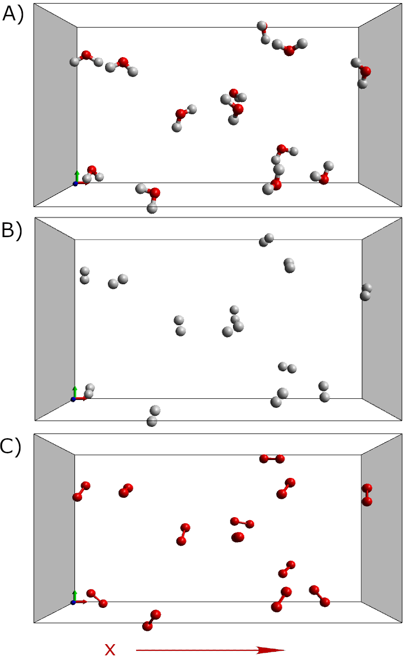
Figure 1: The molecular configurations of targets irradiated by swift protons. A) water vapor; B) H₂ gas; C) O₂ gas. (Color code: oxygen in red; hydrogen in grey.) In each simulation, a swift proton travels through the cell at a given velocity parallel to x-axis.

All the simulations in this work were carried out with the CP2K code. (Hutter et al., 2014; Kühne et al., 2020) To create a sample of water vapor, we first carried out a 25 ps-long adiabatic ab initio molecular dynamics (AIMD) simulation (i.e. within the Born-Oppenheimer regime) of a liquid water sample composed of 104 H₂O molecules in the NVT ensemble at $T=300$ K with a Nosé–Hoover chain thermostat. The electronic structure of the system was treated at the all-electron level within the GAPW scheme implemented in CP2K. We used the 6-311++G(2d2p) basis set and the Perdew-Burke-Ernzerhof exchange-correlation functional. Only the $\Gamma$-point in the electronic Brillouin zone was sampled. The 104 molecules were placed in a periodic cell of dimensions 21.7$\times$12$\times$12 ų, resulting in a liquid water density of 0.996 g/cm³. Then the density of the sample was reduced to 0.1245 g/cm³ by scaling the coordinates of the center-of-mass of each H₂O molecule and duplicating the cell dimensions in the three dimensions. The 13 H₂O molecules still contained within the original cell were selected to represent the water vapor target. The resulting system has a higher density than that of the gas phase at room conditions. The reason for studying water vapor with several water molecules in a box is that we can sample several collisions of various impact parameters in a single simulation. Hence, the sampling efficiency is much higher, compared with sampling all possible impact parameters and molecular orientations with one molecule in the simulation box. An aspect that is not often appreciated is that the cost of periodic-cell simulations, which we use here for technical reasons, grows with the volume of the simulation box. It is therefore more convenient computationally to simulate a smaller box containing more molecules.

After volume scaling, the system was reequilibrated for 5 ps through an additional NVT adiabatic AIMD simulation at $T=300$ K. During this process we fixed the position of the oxygen atoms to avoid collisions between H₂O molecules and the formation of hydrogen-bonded water clusters. Finally, we selected the last configuration of this AIMD run (shown in panel A of Fig. 1) for the ensuing rt-TDDFT simulations.

For convenience, the original samples of hydrogen and oxygen gas were created by replacing each H₂O molecule of the water vapor sample with H₂ or O₂ molecules, respectively. The coordinates of the center-of-mass of each molecule were kept the same. Then, we carried out a 5 ps AIMD simulation under the same conditions to equilibrate the H₂ / O₂ molecules, fixing the centers of mass of the molecules. As before, we selected the last configurations of the trajectories (panels B and C of Fig. 1) for the rt-TDDFT calculations.

2.2 Geometric pre-sampling of short ion trajectories

Since the electronic stopping power is very sensitive to the electronic density, its value depends quite significantly on the specific trajectory of the projectile (Sigmund, 2014; Correa, 2018; Dorado and Flores, 1993; Pruneda et al., 2007; Yao et al., 2019; Gu et al., 2020). In order to obtain a meaningful statistically averaged $S_{e}(E_{k})$ that can be compared to experimental data, it is necessary to run many short trajectories. For targets in condensed phases and randomly selected trajectories, the number of trajectories is on the order of 100 (Yao et al., 2019; Gu et al., 2020). For the gaseous targets studied in this work, it can be expected that more trajectories of similar length are required to achieve an accurate ensemble average of $S_{e}$, as the electronic density in gaseous targets is distributed more sparsely in the simulation box.

To accelerate the convergence of the running average of $S_{e}$, we used our ion trajectory pre-sampling protocol based on a geometric criterion, to ensure that the probability distribution functions (PDFs) of the distance from the ion to the closest atoms, $\phi(r_{p{\rightarrow}x})$ (where $x$ is O or H in this work), accumulated over the selected trajectories, are close enough to the reference PDFs, $\phi_{R}(r_{p{\rightarrow}x})$, calculated with 50,000 randomly selected trajectories (Gu et al., 2020). To evaluate the similarity between $\phi(r_{p{\rightarrow}x})$, calculated for of a set of trajectories, and $\phi_{R}(r_{p{\rightarrow}x})$, we define the overlap index:

$$\cap_{x}=1-0.5\times\int\left|\phi(r_{p{\rightarrow}x})-\phi_{R}(r_{p{\rightarrow}x})\right|dr_{p}$$ (2)

which corresponds to the overlap in the area under the two PDF curves. As the number of selected trajectories (and hence the total accumulated length) increases, all overlap indices approach 1.

For liquid water, a set of 10 short trajectories (about 20 Å-long each) proved sufficient to converge the running average of $S_{e}$ at the Bragg peak, where the most important dependence of $S_{e}$ on the trajectory is observed (Gu et al., 2020). Hence, they can be safely used for carrying out all rt-TDDFT simulations for different ion velocities.

Since our simulations were performed under periodic boundary conditions (PBC) the length of the projectile’s trajectories analyzed was contained within a single unit cell in order to avoid over-excitations produced by the repeated irradiation of the same regions. In addition, to prevent the perturbations by excited electrons in neighboring PBC images, a 6 Å-wide vacuum slab was added between neighboring PBC images along the $x$-direction, which is parallel to the projectile’s trajectory.

In each rt-TDDFT simulation, the proton was initially located at the center of the vacuum region and set in motion by applying an instantaneous kick along the $x$-direction. Then the projectile was allowed to evolve in rectilinear motion for 24.7 Å at the constant given velocity. The portion of the trajectory used to compute $S_{e}$ (and also the PDFs for trajectory selection) is ${\Delta}L=21.7$ Å from $x=3$ Å to 24.7 Å, covering the entire target. In addition, possible violent collisions at the target’s entrance and exit points were avoided by discarding candidate trajectories for which the impact parameter at any of these two points was smaller than $1.2$ Å. Basically, this excludes trajectories that start and/or end with a large variation in the electronic energy ($E_{e}$ in equation 3, below), thus avoiding large uncertainties in the calculated value of $S_{e}$. Such close collision events, however, were not discarded when they happened in the central, much larger, part of the trajectory. An additional concern is that the projectile needs to travel a certain length through the target until its effective charge stabilizes around a certain steady-state value. We have computed the Hirshfeld charge of the projectile along its path and observed that discarding the transient region prior to reaching the steady state, which in the vapor phase of water extends to $\approx$ 6 Å, results in a change of $S_{e}$ of at most 2.5%, and hence we consider that such fluctations in the charge state are irrelevant for the calculation of the stopping power in this case.

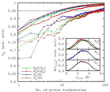
Figure 2: Overlap index $\cap_{x}$ for increasingly long accumulated trajectories generated by geometric pre-sampling (solid lines with dots) and randomly selected ones (dash-dot lines with dots). The same color code is used for both cases. The dotted line at $\cap_{x}=0.95$ is shown as a reference for discussion. The inset shows the PDFs using 25 trajectories for geometry pre-sampling, compared to the reference distributions generated by 50,000 randomly selected trajectories (solid black lines). The color code is the same as above.

As shown in Fig. 2, for both hydrogen and oxygen gas, only 10 pre-sampled trajectories are required to achieve an overlap index of 0.95, while the same overlap index requires about 70 randomly selected trajectories. For water vapor, a few more pre-sampled trajectories (11 for the oxygen PDF, and 16 for hydrogen one) are required to reach $\cap_{x}=0.95$. The observation that more trajectories are required for water vapor can be explained by the fact that, for multi-atomic or multi-species targets, the algorithm selects trajectories that optimize the PDFs of two or more species simultaneously. In this case, the trajectories that optimize the oxygen PDF are not necessarily the optimal ones for optimizing the hydrogen PDF, and vice versa. Therefore, more trajectories are needed to achieve convergence for both species. With random trajectories the overlap index for water vapor is also smaller than for O₂ and H₂ gas. The inset of Fig. 2 shows that the reference PDFs of all atoms in the gaseous targets (black smooth lines) can be reproduced extremely well with 25 pre-selected trajectories.

2.3 Rt-TDDFT simulation and calculation of electronic stopping power

Rt-TDDFT, its applications and numerical implementations have been recently reviewed (Ullrich, 2011; Maitra, 2016). The rt-TDDFT approach was used for the first time to compute electronic stopping power in materials by Pruneda et al. (Pruneda et al., 2007). Since then, other implementations of rt-TDDFT have been proposed in which the projectile with its basis is explicitly included (Correa, 2018). When a projectile is forced to move at a constant speed through a target material, the total energy of the system increases by an amount $\Delta{E}$ as a result of the work done by the constrain to maintain the projectile’s velocity constant (Schleife et al., 2012). For projectile’s kinetic energies large enough, i.e. above a threshold of a few keV/nucleon, the motion of the host nuclei is normally negligible in the time scale of the projectile’s transit due to their large mass. Above the energy threshold, there is no appreciable effect on the electronic dynamics if the host nuclei are constrained to stay at their initial positions during rt-TDDFT stopping simulations. The advantage is that, in this way, the change in total energy is due only to the electronic subsystem, $\Delta{E_{e}}$. The electronic stopping power for a projectile’s trajectory of length $\Delta{L}$ can then be calculated as:

$$S_{e}(E_{k})=\Delta{E_{e}}/\Delta{L}.$$ (3)

For the calculation of the $S_{e}$ of protons by gaseous targets we used the all-electron implementation of rt-TDDFT in CP2K (Hutter et al., 2014; Kühne et al., 2020). As in the equilibration and setup of the system, we used the 6-311++G(2d2p) basis set for target atoms, since for water molecules it produces better results than the 6-311G^∗∗ basis set used in the supplementary information in (Gu et al., 2020). We note that we used the Perdew–Burke–Ernzerhof funcional (Perdew et al., 1996) in its time-local version which does not include memory effects (i.e. the exchange-correlation energy and potential are calculated for the instantaneous density using the standard PBE functional). We remark that the PBE functional has been shown to provide very good estimations of the electronic stopping power in water (Reeves et al., 2016; Yao et al., 2019), and no significant differences have been found between the regular PBE functional and its hybrid version PBE0 (Reeves et al., 2016) or the meta-GGA SCAN functional (Yao et al., 2019).

After placing the proton in its initial position, we obtain the initial Kohn-Sham orbitals, and hence the electronic density, of the system via a regular single-point calculation of the ground state. Then, the rt-TDDFT simulation is initiated by giving an initial velocity to the projectile. This velocity, as well as the position of the target atoms, are maintained unaltered by setting to zero the forces on all nuclei. We called this the Zero Force (ZF) scheme. The time step $\Delta t$ of the real-time propagation was determined by setting a constant displacement of $\Delta x=0.005$ Å in each integration step, i.e. $\Delta t=\Delta x/v$. The largest time step used for our simulations was 0.92 attoseconds, corresponding to the smallest velocity of 0.25 a.u., or energy of 1.56 keV/amu, of the proton.

3 Results and discussion

3.1 Convergence of rt-TDDFT electronic stopping power with pre-sampled ion trajectories.

Using the pre-sampled short trajectories selected in Section 2.2, we calculated the electronic stopping power $S_{e}(E_{k})$ for protons in water vapor, H₂ and O₂ gas for proton kinetic energies $E_{k}$ ranging from 1.56 keV to 1.6 MeV, corresponding to velocities between 0.25 and 8 a.u. This was done by running rt-TDDFT simulations at the theory level and basis set described in Section 2.3. To check the convergence of the averaged $S_{e}$ values in the gaseous targets, we focused on the case $E_{k}=125$ keV/amu. This is precisely the proton energy used in SRIM to determine the reference CAB table, which in turn is used to estimate the electronic stopping power for various ions in different compounds (Ziegler et al., 2010). The rt-TDDFT $S_{e}$ values at 125 keV/amu will be used later to calculate the rt-TDDFT CAB strengths and compare them with SRIM data. In addition, this energy is close to the Bragg peak, where $S_{e}$ is most sensitive to the proton trajectory (Gu et al., 2020).

In Fig. 3 we show, with open circles, the calculated $S_{e}$ values for proton at 125 keV/amu along single pre-sampled short trajectories in the three gaseous targets. A first observation for the three target systems is that the distribution of $S_{e}$ values of the individual trajectories is quite broad, with differences that can be larger than a factor of 20 (mind the logarithmic vertical scale in Fig. 3). Not unexpectedly, comparing such plot with one for an equivalent condensed phase system (Gu et al., 2020) makes it clear that the trajectory dependence of $S_{e}$ is greatly enhanced in the case of gas-phase targets, which must be taken into account when computing statistically averaged quantities.

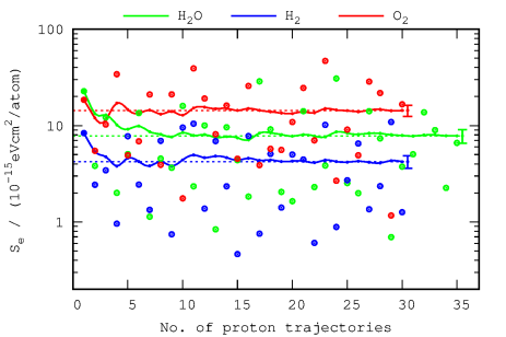
Figure 3: Stopping power 125 keV/amu protons in water vapor (green), and H₂ (blue) and O₂ (red) gas, calculated with 21.7 Å-long pre-sampled trajectories. The individual $S_{e}$ values for each trajectory are indicated with open circles. The running averages of $S_{e}$ are shown with solid lines, and standard deviations are shown as a vertical tick to the right of each line. The average $S_{e}$ values converged over 30 trajectories for H₂ and O₂ and 35 trajectories for water vapor are indicated with dashed lines.

The converged averages of $S_{e}$ for H₂O, H₂ and O₂ are $7.8\times 10^{-15}$, $4.2\times 10^{-15}$ and $14.3\times 10^{-15}$ eVcm²/atom, respectively. They were obtained using 35, 30 and 30 pre-sampled trajectories. These values were converged already with 28, 22 and 22 trajectories, remaining stable within $\pm$3% upon increasing the sampling, and with final estimated standard deviations of $\pm 8\mathrm{\sim}10\%$ as indicated in Fig. 3. We note that we express $S_{e}$ in units of eVcm²/atom as customarily done in the radiation damage field, which has the advantage of being independent of the density of the target system and thus facilitates the comparison with different systems or phase states.

Simulations conducted at other energies showed that the number of selected short trajectories required for this same level of convergence of $S_{e}(E_{k})$ is less than 30 for water vapor and less than 25 for both oxygen and hydrogen in gas phase. However, for the sake of consistency and in order to ensure an utmost statistical accuracy, in the following calculations of rt-TDDFT $S_{e}(E_{k})$ curves we imposed a tighter convergence criterion and used 35 pre-selected short trajectories for water vapor and 30 for hydrogen and oxygen gas.

3.2 Electronic stopping powers for proton in water vapor, and hydrogen and oxygen gases

The rt-TDDFT $S_{e}(E_{k})$ curves for H₂O, H₂ and O₂ targets calculated using the pre-sampled trajectories are reported in Fig. 4, along with the corresponding SRIM curves (Ziegler et al., 2010) and the available experimental data (Montanari, ).

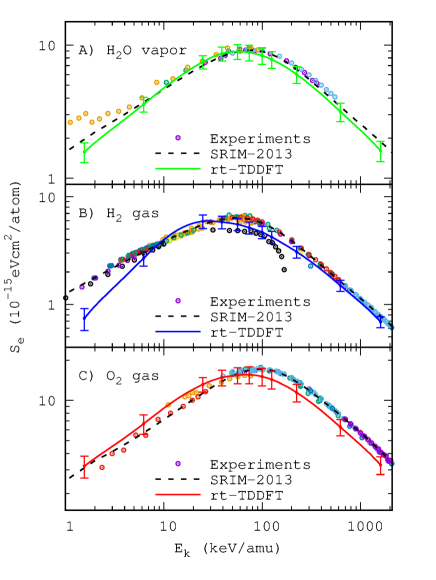
Figure 4: Electronic stopping power curves for proton by A) water vapor, B) H₂ gas and C) O₂ gas. The rt-TDDFT curves are show as solid lines with error bars indicating the standard deviation of the averaged values of short ion trajectories. The corresponding SRIM-2013 curves (Ziegler et al., 2010) are shown as black dashed lines. The experimental values for the corresponding targets are shown as open circles in different colors for the various sources (see details in (Montanari, ) and references therein).

For water vapor the rt-TDDFT electronic stopping curve (Fig. 4A) coincides with the SRIM curve and with the experimental data to an excellent extent, except at very low energies. When compared to SRIM, the position of the Bragg peak in the rt-TDDFT curve is red-shifted by 15 keV/amu, from $E_{k}=75$ to $60$ keV/amu, and the peak value of $S_{e}$ is underestimated in $0.34\times\mathrm{10^{-15}eVcm^{2}/atom}$, i.e. a 4%. In a previous work, we calculated the $S_{e}$ curve for protons in liquid water, using the (smaller) 6-311G** basis set and found that the position of the Bragg peak in rt-TDDFT $S_{e}$ curve was also red-shifted by 15 keV/amu, and the peak value of $S_{e}$ was underestimated by a similar 4%  (Gu et al., 2020).

To assess the contribution of the additional diffuse and polarization functions included in the present basis set, 6-311++G(2d2p), but absent in 6-311G**, we re-calculated the $S_{e}$ curve for protons in liquid water with the new basis, using 16 pre-sampled ion trajectories for the liquid water sample composed of 104 molecules. The effect of the additional basis functions is to reduce the red shift of the Bragg peak relative to SRIM to 5 keV/amu, and the underestimation of the peak height to less than 2%. These results indicate that the accuracy of $S_{e}$ calculated by rt-TDDFT simulations with Gaussian basis sets can be increased by improving the basis, as discussed in the Supplementary Information in (Gu et al., 2020). However, the absolute quality of the calculated $S_{e}$ for a given basis set depends on the phase state, whether gas or condensed, and more generally on the density of the target material. Specifically, a larger basis set is required to achieve the same accuracy in water vapor than in liquid water or ice.

In the low energy end, when $E_{k}<5$ keV/amu, the rt-TDDFT stopping values for water vapor fall below the experimental data and the empirical SRIM data, with the relative difference increasing as $E_{k}$ decreases. The underestimation of rt-TDDFT $S_{e}$ at low energies becomes even larger when we take into account the red shift due to basis set effects. The red shift can be observed clearly in the high-energy end of Fig. 4A, where the rt-TDDFT results (solid green line) lie to the left of SRIM (dashed line) and experiment (open circles). This effect has also been reported for other targets in TDDFT (Schleife et al., 2015; Maliyov et al., 2018; Gu et al., 2020) and quantum Monte Carlo calculations (Alcocer-Ávila et al., 2019). If we shift the rt-TDDFT curve to the right to make it coincide with experiment and SRIM, then the values at low energies become even lower, thus enhancing the underestimation of $S_{e}$ in that region.

A reason for this underestimation of the electronic stopping by rt-TDDFT calculations may be the possible deviation of the trajectories due to small impact parameter collisions with the target atoms (Muñoz Santiburcio, ). Because of these deflections, the projectiles sampled in the experiments after passing a material with a given thickness would have experienced repeated changes of trajectory, thus allowing them to deposit more energy in the material than if the trajectory were rectilinear, as assumed in the ZF approximation. Therefore, we can establish the existence of a threshold energy, $E_{\text{min-ZF}}$, for the validity of the ZF scheme. $E_{\text{min-ZF}}$ should be larger than the energy at which the rt-TDDFT curve and experimental and/or empirical data intersect. According to Fig. 4A, for water vapor $E_{\text{min-ZF}}>5$ keV/amu.

In addition, we note that the experimental stopping power for $E_{k}<100$ keV/amu shown in open circles in Fig. 4A, was derived by measuring the ionization range of protons in water vapor applying the continuous slowing-down approximation (CSDA) (Baek et al., 2006). The measured stopping power appears larger than the electronic stopping power as the relative contribution of nuclear stopping increases when $E_{k}$ decreases. It is worth mentioning that theoretically GEANT4-DNA is suggested to be only suitable for the calculation of stopping and range of protons in liquid water when $E_{k}>5$ keV/amu, since nuclear stopping is neglected in the program (Francis et al., 2011b). Clearly, more experimental efforts addressing this important system in this energy range would be welcome.

For hydrogen gas, the rt-TDDFT value of stopping at the Bragg peak is $6.27\times\mathrm{10^{-15}eVcm^{2}/atom}$, which is very close to the SRIM value of $6.35\times\mathrm{10^{-15}eVcm^{2}/atom}$, i.e. within a 1%. The maximum, however, is located at an energy of 26 keV/amu ($v_{p}=1.02$ a.u.), which is much smaller than the value of 55 keV/amu ($v_{p}=1.5$ a.u.) reported by SRIM and experiments. As $E_{k}$ increases the rt-TDDFT $S_{e}$ curve progressively approaches experimental data and SRIM. On the contrary, as $E_{k}$ decreases the rt-TDDFT $S_{e}$ curve decreases much faster than experimental data and SRIM, especially below $E_{k}<10$ keV/amu. The situation is similar to, but much more dramatic than for water vapor. Also in this case the discrepancy between rt-TDDFT calculations and experimental data can be understood in terms of the limitations imposed by the ZF scheme that does not include trajectories that have scattered from the nuclei.

Therefore, for H₂ gas the threshold energy for the validity of the ZF scheme is $E_{\text{min-ZF}}>10$ keV/amu, quite higher than for water vapor. This is consistent with calculations for a hydrogen beam colliding with molecular hydrogen by Cabrera-Trujillo et al, which showed that for projectile energies between 10 and 25 keV/amu, the nuclear and rovibrational contribution of the molecular target introduces an angular dependence on the experimental stopping cross section (Cabrera-Trujillo et al., 2002). To determine the exact value of $E_{\text{min-ZF}}$, we should go beyond the ZF approximation and disentangle the nuclear and electronic contributions to stopping accurately with a different scheme. This is still a challenge for ab initio calculations.

For oxygen gas, the shape of the rt-TDDFT $S_{e}$ curve as a whole is consistent with the SRIM curve and experimental data, especially in the low energy region where the ZF approximation becomes questionable for water vapor and hydrogen gas. It is clearly shown that for oxygen gas the threshold energy for the validity of the ZF scheme is lower than for the other two cases, arguably below the lowest energy studied in this work (1.56 keV/amu). We noticed that at the low energy end, the experimental electronic stopping power for protons, shown as red circles in Fig.4C, was derived by subtracting the theoretical nuclear stopping powers from the total stopping measured using a differentially pumped stopping cell (Børgesen, 1985). Hence those results are substantially lower at low energies compared to values derived from range measurements. In addition, while the shape of the rt-TDDFT $S_{e}$ curve is well reproduced, there is a noticeable red-shift of the whole curve; the rt-TDDFT Bragg peak for protons in oxygen gas is $15.58\times\mathrm{10^{-15}eVcm^{2}/atom}$, which is lower than the SRIM value of $17.15\times\mathrm{10^{-15}eVcm^{2}/atom}$ by 9%. The position of the rt-TDDFT Bragg peak is red-shifted by 25 keV/amu from 100 keV/amu ($v_{p}=2.0$ a.u.) of SRIM to 75 keV/amu ($v_{p}=1.73$ a.u.) of the rt-TDDFT calculation. As pointed out above, we have already established that this red shift is mainly related to basis set convergence.

In this work, the number density of molecules of the three targets are set to be equal. Therefore, the ratio of the number density of electrons, $\rho_{e}$, is 16:10:2 for O₂, H₂O and H₂, respectively. As can be seen in Fig. 4, at high energy, where the ZF scheme is perfectly suitable, the magnitude of the red-shift, $\delta{E_{k}}=[E_{k(\mathrm{ref})}(S_{e})-E_{k(\mathrm{rt-TDDFT})}(S_{e})]$ for a given $S_{e}$ value, increases with $\rho_{e}$ according to $\delta{E_{k}}[\mathrm{H}_{2}]<\delta{E_{k}}[\mathrm{H}_{2}\mathrm{O}]<\delta{E_{k}}[\mathrm{O}_{2}]$. The fact that $\delta(E_{k})$ is positively correlated with $\rho_{e}$ constitutes further evidence that the red-shift is related to the completeness of the basis set. In addition, these results suggest that the basis set for hydrogen seems closer to completeness than that for oxygen.

It should be mentioned that the rt-TDDFT $S_{e}$ curves in Fig. 4 are all calculated based on the restricted Kohn-Sham (RKS) approximation (Kohanoff, 2006). This means the channels for spin flipping and related electronic excitations have been neglected. We note that we tested the effect of using the unrestricted Kohn-Sham (UKS) scheme for the case of the O₂ molecule (which actually could be thought to be imperative since such formalism is required to obtain the triplet ground state of O₂), finding out that both RKS and UKS produce quite similar $S_{e}$ values, which justifies the use of RKS over UKS given the smaller computational cost for the already expensive determination of S_e via rt-TDDFT. In any case, a suitable scheme for the propagation of the time-dependent Kohn-Sham orbitals should allow for spin-flipping channels. In the present calculations this was not implemented and, hence, any such excitations were absent. This may explain the underestimation of $S_{e}$ for O₂ gas. Simulation techniques to incorporate these excitations are still under development (Kühne et al., 2020; Casanova and Krylov, 2020).

3.3 Bragg’s additivity rule: from hydrogen and oxygen to water

The assumption of BAR is that the stopping power in a compound can be approximately calculated as the stoichiometric sum of the stopping powers of its elementary components:

$$S_{e}^{\mathrm{BAR}}(E_{k})=\sum{r_{\mathrm{x}}}~{}{S}_{e}{[\mathrm{x}]}(E_{k}),$$ (4)

in which $r_{\mathrm{x}}$ is the ratio of the number density of the atomic species $\mathrm{x}$ to the total number density of all atoms in the target. ${S}_{e}{[\mathrm{x}]}(E_{k})$ is the stopping power in the elemental material of species $\mathrm{x}$. This expression carries the implicit assumption that the physical phase (e.g. solid vs liquid) of the stopping medium and the chemical bonding of atoms into molecules have negligible influence on the mean energy loss.

However, differences in electronic structure in going from free atoms to molecules cannot be neglected, especially in the low energy regime, where the relative contribution of valence (outer shell or bonding) electrons to the stopping power is large. This is also the case of light elements whose valence electrons are a major fraction of the total. Under those circumstances, the validity of the BAR becomes questionable (Thwaites, 1983). A measure of the bonding contribution is given by the difference in (measured or calculated), stopping power relative to the BAR approximation, i.e.

$$\Gamma(E_{k})=[1-S_{e}(E_{k})/S_{e}^{\mathrm{BAR}}(E_{k})]\times 100\%.$$ (5)

In practice, the concept of elementary material, as used by SRIM, refers to stable forms of the element in the gas phase, which in many cases corresponds to simple molecules instead of isolated atoms. For H₂O, they are O₂ and H₂. Therefore, the bonding contribution in equation (5) is the relative variation of $S_{e}$ as the target changes from a mixture of the elementary molecular species, to the compound.

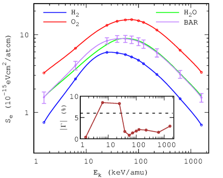
Figure 5: The BAR additivity of rt-TDDFT electronic stopping power $S_{e}(E_{k})$, according to formula of $\mathrm{2H_{2}+O_{2}{\rightarrow}2H_{2}O}$. The rt-TDDFT $S_{e}(E_{k})$ curves for H₂ gas and O₂ gas, and water vapor are shown with blue, red and green lines individually. The BAR curve is given as purple line with error bar. The inset shows the relative scaling factor $\Gamma$ obtained from rt-TDDFT (brown dots and line), along with the constant scaling value recommended by SRIM (black dashed line).

We used the results of Fig. 4 to assess the validity of Bragg’s additivity for the electronic stopping of water calculated by rt-TDDFT, where the mixing is decribed by the reaction $\mathrm{2H_{2}+O_{2}{\rightarrow}2H_{2}O}$. The resulting curves are reported in Fig. 5. The error bars are calculated as the sum of those for O₂ and H₂ (see Fig. 4). As shown in the inset to Fig. 5, when $E_{k}>40$ keV/amu ($v_{p}>1.25$ a.u), the relative scaling factor $\Gamma$ stays below $\pm$3%, which is below the statistical error of rt-TDDFT $S_{eBAR}$. This means that BAR is supported by parameter-free rt-TDDFT calculations without further scaling, in the medium- to high-energy regime, including the Bragg peak at 72 keV/amu. When $E_{k}$ decreases below 40 keV/amu, $S_{eBAR}$ is larger than the $S_{e}$ calculated directly. $\Gamma(E_{k})$ first increases to $\sim 8.5$% for $E_{k}=20$ keV/amu and $E_{k}=5$ keV/amu, and then decreases to almost zero on the low energy end of $E_{k}=1.56$ keV/amu.

It is important to remark that the energy dependence of $\Gamma(E_{k})$ is quite different from that used in SRIM. In the latter, from H₂ and O₂ to water, $\Gamma$ is assumed to be 6%, independently of the projectile’s energy. This value is obtained by scaling the BAR curve to reproduce experimental data, if available, or otherwise the CAB value for a compound at the Bragg peak, and then it is assumed to be valid at all velocities. Our results indicate that this may not be the most suitable approximation to $\Gamma$.

It has been mentioned in Section 3.2 that, on the low-energy end, the rt-TDDFT $S_{e}$ calculated within the ZF approximation is underestimated with respect to experiments. This makes difficult the comparison of the calculated $\Gamma(E_{k})$ with that arising from experimental data. Nevertheless, the decrease of $\Gamma(E_{k})$, which is inconsistent with the notion that the chemical bonding contribution to electronic stopping should emerge clearly in the low-energy regime, implies that electron-nuclear coupling is important for light targets and low velocities.

3.4 Core and bond (CAB) electronic stopping powers

The SRIM CAB table was calculated according to the following prescription (Ziegler et al., 2010; Ziegler and Biersack, 2008). Firstly, the experimental data points available for different ions at various velocities and in different materials were scaled to the equivalent value corresponding to protons at 125 keV/amu, assuming that the effective charge of the ion does not depend on the target material, but only the energy of the ion. Next, the core and bond contributions for protons at 125 keV/amu were disentangled by solving the system of linear equations

$$S_{e}^{\mathrm{CAB}}(E_{k})=\sum{S_{e}[X]}+\sum{S_{e}[Y]},$$ (6)

in which [X] indicates the ionic core, i.e. nuclei plus core electrons and [Y] refers to the inter-atomic chemical bonds in the target material, involving only valence electrons. For example, for a CO molecule $S_{e}^{\mathrm{CAB}}=S_{e}[$C$]+S_{e}[$O$]+S_{e}[$C$\equiv$O$]$. Finally, the whole stopping power curve as a function of the energy (or velocity) of the ion was generated by scaling the BAR curve with the ratio of ${S_{e}}/{S_{e}}^{\mathrm{BAR}}$ for protons at 125 keV/amu, and multiplying with the following asymptotic function

$$f(v_{1})=\left\{1+\exp\left[1.47\left(\frac{v_{1}}{v_{0}}-7.0\right)\right]\right\}^{-1},$$ (7)

with $v_{0}=1$ a.u., corresponding to 25 keV/amu, to ensure that the deviation from the BAR curve vanishes at high energies (Ziegler and Manoyan, 1988).

Based on rt-TDDFT calculations of $S_{e}$ for protons at 125 keV/amu in different compounds, the CAB contributions to electronic stopping powers can be directly disentangled by solving a system of linear equations, without resorting to a general fitting as it is done in SRIM. Here we calculated the rt-TDDFT core and bond contributions of hydrogen and oxygen in water, and compared them to SRIM published tables.

In addition to water vapor and H₂ and O₂ gases, we included also a calculation of the stopping power for protons in hydrogen peroxide (H₂O₂), with the same procedure, theory level and basis set used for O₂ and H₂ gases, as discussed in Section 2. This introduces a different type of bond between two oxygen atoms (O-O), weaker than that in O₂ (O=O). On the other hand, since the hydrogen electron always participates in a chemical bond, it is reasonable to follow the rule used in SRIM, i.e. taking the core contribution of the hydrogen atom $S_{e}[\mathrm{H}]$ as zero. According to Eq. (6), the rt-TDDFT stopping values for H₂, O₂, H₂O and H₂O₂ can be combined in the following set of four linear equations in five unknowns:

$$\begin{cases}S_{e}[\mathrm{H_{2}}]=S_{e}[\mathrm{H\text{-}H}]=8.46\pm 0.61\\ S_{e}[\mathrm{O_{2}}]=2S_{e}[\mathrm{O}]+S_{e}[\mathrm{O\text{=}O}]=28.68\pm 2.13\\ S_{e}[\mathrm{H_{2}O}]=S_{e}[\mathrm{O}]+2S_{e}[\mathrm{O\text{-}H}]=23.41\pm 1.90\\ S_{e}[\mathrm{H_{2}O_{2}}]=2S_{e}[\mathrm{O}]+2S_{e}[\mathrm{O\text{-}H}]+S_{e}[\mathrm{O\text{-}O}]=33.55\pm 3.13\end{cases}$$ (8)

where the stopping power is expressed in $\mathrm{10^{-15}eVcm^{2}/unit}$, being ‘unit’ an atom, bond, or molecule. This set of equations has an infinite line of possible solutions. In order to obtain a unique solution, we fixed the ratio $S_{e}[\mathrm{O}]/S_{e}[\mathrm{O\text{=}O}]$ to the SRIM value, thus reducing the system to four equations in four unknowns. The calculated uncertainties are also decomposed into core and bond contributions according to their stoichiometric coefficients in Eq. (8).

Table 1: Hydrogen and oxygen related CAB contributions to electronic stopping power calculated by rt-TDDFT simulations and SRIM-2013 (Ziegler et al., 2010). The unit of stopping power is $\mathrm{10^{-15}eVcm^{2}/(atom~{}or~{}bond).}$ The last column reports the relative percentual difference between rt-TDDFT and SRIM.

	Name	rt-TDDFT	SRIM-2013	$\epsilon(\%)$
Core	H	0	0	0
	O	4.68$\pm 0.35$	5.36	-12.6
Bond	H-H	8.46$\pm 0.61$	10.049	-15.8
	H-O	$9.37\pm 0.77$	10.085	-7.1
	O-O	5.$1\pm$1.27	–	–
	O=O	19.24$\pm 1.43$	22.044	-12.6

The CAB contributions to the calculated rt-TDDFT stoppings, along with the SRIM-2013 data, are presented in Table 1. On the other hand, as shown in Fig. 2, at $E_{k}=125~{}\mathrm{KeV/amu}$ all the values of rt-TDDFT $S_{e}$ are underestimated relative to SRIM. Hence, all the rt-TDDFT CAB values are smaller than the corresponding SRIM data by more than 10%, except the O-H bond which is only about 7% smaller, as a consequence of the calculated $S_{e}$ for H₂O being the closest one to SRIM (Fig. 2).

For O₂ the discrepancies between rt-TDDFT results and experimental data are due to the basis set effect discussed above, which induces a red-shift in the rt-TDDFT curve. For H₂, in that energy region the ZF approximation is probably valid, but there is an obvious discrepancy between different sets of experimental data. SRIM follows one set, which runs slightly above rt-TDDFT calculations, and this may contribute to the underestimation.

It should also be noticed that, in the region of the Bragg peak, stopping powers for protons and $\alpha$-particles in water and organic materials in the vapor phase are often larger than in the liquid or solid state by up to 5-10%. The phase effect in $S_{e}$ is considered to be due largely to changes in electronic excitation levels across the phase transition (Thwaites, 1992). For liquid water and water vapor, the difference arises from the presence or absence of hydrogen bonds between the water molecules. In practice, by scaling up the size of the box from liquid water, the O$\cdots$H distances become larger than 4 Å, well longer than the typical 1.8–2.6 Å, so that hydrogen-bonding interactions are negligible. Therefore, we argue that the vapor state is very well-represented in the current approach and we consider that the error associated to using such density is negligible. To substantiate this assertion, we have run tests at a lower density, and observed no significant differences.

Interestingly, for both rt-TDDFT calculations and SRIM, the magnitude of the bond contributions reported in Table 1 follows the order: $S_{e}[\text{O=O}]>S_{e}[\text{H-O}]>S_{e}[\text{H-H}]>S_{e}[\text{O-O}]$. Notice that $S_{e}[\text{O-O}]$ is not provided by SRIM, though. This order is consistent with that of the average bond energies for these bonds (Luo, 2007). For example, the O-O bond strength is 142 kJ/mol and its average rt-TDDFT $S_{e}$ value is quite small, at $5.1\times\mathrm{10^{-15}eVcm^{2}/bond}$. In contrast, the bond energy of the O=O double bond, the strongest one in the table, is 494 kJ/mol, which correlates with a larger contribution to stopping power, i.e. $19.24\times\mathrm{10^{-15}eVcm^{2}/bond}$ according to rt-TDDFT simulations. This correlation suggests that the bond contribution to the electronic stopping power is proportional to chemical bond strength, which is reasonable as stopping is known to increase with electronic density. This observation is consistent with more elaborate addition schemes in which the stopping of the compound depends on the number of valence electrons (Sigmund and Schinner, 2018).

It is important to remark that this decomposition depends heavily on the bonds included in the fit. For example, if we ignore the O-O bond by setting $S_{e}[\text{O-O}]=0$, while keeping the last equation in (8), the $S_{e}[\text{O}]$ core contribution increases to compensate for the missing bond term. If we set the unrealistic condition that $S_{e}[\text{O-O}]=S_{e}[\text{O=O}]$, then the other core and bond contributions decrease. One could also ignore the equation for H₂O₂ in (8). In that case the core and bond contributions are similar to the original ones, except that there is no bond contribution for O-O.

4 Conclusions and perspectives

Rt-TDDFT simulations are by now a well-established tool to compute electronic stopping in complex systems directly, when experimental data are not available or incomplete. Moreover, they can be used to calculate the stopping for elements or simple molecules, thus forming a data base to compute stopping power in general complex systems via additivity rules.

In this work, electronic stopping power curves for energetic protons in water vapor, hydrogen and oxygen gas, were calculated via rt-TDDFT simulations, as a function of the kinetic energy of the proton. The approach used the zero force approximation, and a recently developed geometric pre-sampling technique to select the projectile’s trajectories. We found that, for these gaseous targets, a number of 25-30 optimally selected, 2 nm-long ion trajectories, are required to converge the average of $S_{e}(E_{k})$ within a 3%. The obtained values can be compared directly with experimental data.

For water vapor and hydrogen gas, in the high-energy region, the rt-TDDFT Bragg peak value and the shape of $S_{e}(E_{k})$ curve are consistent with experimental data. On the other hand, at low energies, below a threshold of 5 keV/amu for water vapor and $\sim 20$ keV/amu for H₂ gas, rt-TDDFT stopping is underestimated compared to experimental data. The discrepancies are consistent with the introduction of the zero force scheme, which neglects scattering of low velocity ions by nuclei. This is especially important for light atoms like H, which are present in H₂ and H₂O, but not in O₂. For O₂ gas, there is a clear red shift of the rt-TDDFT $S_{e}(E_{k})$ curve compared to experimental data, much more than for water vapor and H₂ gas. We ascribe this to basis set convergence effects.

Bragg’s additivity rule for the $\mathrm{2H_{2}+O_{2}{\rightarrow}2\,H_{2}O}$ system was found to be applicable to rt-TDDFT electronic stopping values without scaling, when $E_{k}>40$ keV/amu. Our results indicate that the scaling factor depends on velocity, hence suggesting that the constant 6% scaling proposed by SRIM for water may not be the most suitable approximation. The rt-TDDFT core and bond electronic stopping contributions are smaller than those derived from SRIM data, as a result of the red shift of rt-TDDFT $S_{e}(E_{k})$ curves, but the relative weights of the core and bond contributions are consistent between the two methodologies, thus further cross-validating the approach.

Therefore, to increase the general accuracy of rt-TDDFT calculations of electronic stopping power with high efficiency, it is worth focusing on the following two aspects. In the first place, the red-shift of the $S_{e}$ curves might be mitigated by increasing the basis set size, by designing optimal Gaussian basis sets for this type of application (Maliyov et al., 2020), or by using plane wave methods and sufficiently high cutoffs (Correa, 2018), possibly via GPU implementations (Andrade et al., 2021). Secondly, for light targets and low ion velocity regime, one should move away from the zero force approximation and allow for the target atoms to move, e.g. via Ehrenfest dynamics. This will most likely require a modification of the geometric sampling algorithm, which should be designed to include corrections for non-rectilinear trajectories  (Cabrera-Trujillo et al., 2002).

The SRIM CAB table for light compounds includes the elements: H, C, N, O, F, S, and Cl, and was fitted to experimental data on 114 different compounds (Ziegler et al., 2010). To move into that direction we are carrying out additional rt-TDDFT simulations for a set of relatively simple molecules including the other elements, e.g. CO₂, CH₄, etc.

In addition to additivity of stopping power from elementary atoms to molecules, simple organic molecules can also be used as units to calculate stopping power for complex targets such as DNA and other biomolecules like proteins (Sauer et al., 2019). In this case, instead of core and bond, we would have a superposition of intrinsic contributions from individual molecules, and contributions from bonds between molecular units. These can be covalent or hydrogen bonds.

Declaration of competing interest

The authors declare that they have no known competing financial interests or personal relationships that could have appeared to influence the work reported in this paper.

References

- Alcocer-Ávila et al. (2019) Alcocer-Ávila, M.E., Quinto, M.A., Monti, J.M., Rivarola, R.D., Champion, C., 2019. Proton transport modeling in a realistic biological environment by using TILDA-V. Sci. Rep. 9.
- Andersen and Ziegler (1977) Andersen, H.H., Ziegler, J.F., 1977. Hydrogen. Stopping powers and ranges in all elements. Pergamon Press.
- Andrade et al. (2021) Andrade, X., Pemmaraju, C.D., Kartsev, A., Xiao, J., Lindenberg, A., Rajpurohit, S., Tan, L.Z., Ogitsu, T., Correa, A.A., 2021. INQ, a modern gpu-accelerated computational framework for (time-dependent) density functional theory. arXiv preprint arXiv:2106.03872 .
- Apostolakis et al. (2015) Apostolakis, J., Asai, M., Bagulya, A., Brown, J.M.C., Burkhardt, H., Chikuma, N., Cortes-Giraldo, M.A., Elles, S., Grichine, V., Guatelli, S., Incerti, S., Ivanchenko, V.N., Jacquemier, J., Kadri, O., Maire, M., Pandola, L., Sawkey, D., Toshito, T., Urban, L., Yamashita, T., 2015. Progress in geant4 electromagnetic physics modelling and validation. Journal of Physics: Conference Series 664, 072021.
- Baek et al. (2006) Baek, W., Grosswendt, B., Willems, G., 2006. Ionization ranges of protons in water vapour in the energy range 1–100 kev. Radiation protection dosimetry 122, 32–35.
- Baskar et al. (2012) Baskar, R., Lee, K.A., Yeo, R., Yeoh, K.W., 2012. Cancer and radiation therapy: Current advances and future directions. Int. J. Med. Sci. 9, 193–199.
- Bauer et al. (1994) Bauer, P., Käferböck, W., Nečas, V., 1994. Investigation of the electronic energy loss of hydrogen ions in h2o: influence of the state of aggregation. Nuclear Instruments and Methods in Physics Research Section B: Beam Interactions with Materials and Atoms 93, 132–136.
- Bernal et al. (2015) Bernal, M.A., Bordage, M.C., Brown, J.M.C., et al., 2015. Track structure modeling in liquid water: A review of the Geant4-DNA very low energy extension of the Geant4 Monte Carlo simulation toolkit. Physica Medica 31, 861–74.
- Bohr (1913) Bohr, N., 1913. On the theory of the decrease of velocity of moving electrified particles on passing through matter. London, Edinburgh, Dublin Philos. Mag. J. Sci. 25, 10–31.
- Børgesen (1985) Børgesen, P., 1985. Measurements of the stopping power for kev light ions in condensed molecular gases. Nuclear Instruments and Methods in Physics Research Section B: Beam Interactions with Materials and Atoms 12, 73–79.
- Both et al. (1983) Both, G., Krotz, R., Lohmer, K., Neuwirth, W., 1983. Density dependence of stopping cross sections measured in liquid ethane. Phys. Rev. A 28, 3212–3216.
- Bragg and Kleeman (1905) Bragg, W.H., Kleeman, R., 1905. On the particles of radium, and their loss of range in passing through various atoms and molecules . London, Edinburgh, Dublin Philos. Mag. J. Sci. 10, 318–340.
- Cabrera-Trujillo and Hachimi (2020) Cabrera-Trujillo, R., Hachimi, A.G.E., 2020. Calculation of the electronic, nuclear, rotational, and vibrational stopping cross sections for h atoms irradiation on H2, N2 and O2 gas targets at low collision energies. Journal of Physics B: Atomic, Molecular and Optical Physics 53, 135203.
- Cabrera-Trujillo et al. (2002) Cabrera-Trujillo, R., Öhrn, Y., Deumens, E., Sabin, J.R., 2002. Trajectory and molecular binding effects in stopping cross section for hydrogen beams on H2. J. Chem. Phys. 116, 2783–2793.
- Calcagno et al. (1992) Calcagno, L., Compagnini, G., Foti, G., 1992. Structural modification of polymer films by ion irradiation. Nucl. Inst. Methods Phys. Res. B 65, 413–422.
- Casanova and Krylov (2020) Casanova, D., Krylov, A.I., 2020. Spin-flip methods in quantum chemistry. Physical Chemistry Chemical Physics 22, 4326–4342.
- Chen (2010) Chen, J., 2010. Microdosimetric characteristics of proton beams from 50 keV to 200 MeV. Radiation Protection Dosimetry 143, 436–439.
- Correa (2018) Correa, A.A., 2018. Calculating electronic stopping power in materials from first principles. Comput. Mater. Sci. 150, 291–303.
- Correa et al. (2012) Correa, A.A., Kohanoff, J., Artacho, E., Sánchez-Portal, D., Caro, A., 2012. Nonadiabatic forces in ion-solid interactions: The initial stages of radiation damage. Phys. Rev. Lett. 108, 213201.
- Cucinotta et al. (2012) Cucinotta, F.A., Kim, M.H.Y., Chappell, L.J., 2012. Evaluating shielding approaches to reduce space radiation cancer risks. NASA Technical Memorandum 217361.
- Da Pieve et al. (2021) Da Pieve, F., Gronoff, G., Guo, J., Mertens, C.J., Neary, L., Gu, B., Koval, N.E., Kohanoff, J., Vandaele, A.C., Cleri, F., 2021. Radiation environment and doses on mars at oxia planum and mawrth vallis: Support for exploration at sites with high biosignature preservation potential. Journal of Geophysical Research: Planets 126, e2020JE006488.
- Dorado and Flores (1993) Dorado, J.J., Flores, F., 1993. Molecular-orbital theory for the stopping power of atoms in the low-velocity regime: The case of helium in alkali metals. Phys. Rev. A 47, 3062–3072.
- Durante and Parodi (2020) Durante, M., Parodi, K., 2020. Radioactive beams in particle therapy: Past, present, and future. Frontiers in Physics 8, 326.
- EJ (1978) EJ, H., 1978. LET and RBE. In: Radiobiology for the radiologist. Philadelphia: Harper Row, Publishers.
- Ferrari and Szuszkiewicz (2009) Ferrari, F., Szuszkiewicz, E., 2009. Cosmic rays: a review for astrobiologists. Astrobiology 9, 413–436.
- Francis et al. (2011a) Francis, Z., Incerti, S., Karamitros, M., Tran, H., Villagrasa, C., 2011a. Stopping power and ranges of electrons, protons and alpha particles in liquid water using the geant4-dna package. Nuclear Instruments and Methods in Physics Research Section B: Beam Interactions with Materials and Atoms 269, 2307–2311. 12th International Conference on Nuclear Microprobe Technology and Applications.
- Francis et al. (2011b) Francis, Z., Incerti, S., Karamitros, M., Tran, H., Villagrasa, C., 2011b. Stopping power and ranges of electrons, protons and alpha particles in liquid water using the geant4-dna package. Nuclear Instruments and Methods in Physics Research Section B: Beam Interactions with Materials and Atoms 269, 2307–2311.
- Friedland et al. (2017) Friedland, W., Schmitt, E., Kundrát, P., Dingfelder, M., Baiocco, G., Barbieri, S., Ottolenghi, A., 2017. Comprehensive track-structure based evaluation of dna damage by light ions from radiotherapy-relevant energies down to stopping. Scientific reports 7, 1–15.
- Granberg et al. (2016) Granberg, F., Nordlund, K., Ullah, M.W., Jin, K., Lu, C., Bei, H., Wang, L.M., Djurabekova, F., Weber, W.J., Zhang, Y., 2016. Mechanism of radiation damage reduction in equiatomic multicomponent single phase alloys. Phys. Rev. Lett. 116, 135504.
- Gu et al. (2020) Gu, B., Cunningham, B., Muñoz Santiburcio, D., Da Pieve, F., Artacho, E., Kohanoff, J., 2020. Efficient ab initio calculation of electronic stopping in disordered systems via geometry pre-sampling: Application to liquid water. J. Chem. Phys. 153, 034113.
- Hutter et al. (2014) Hutter, J., Iannuzzi, M., Schiffmann, F., Vandevondele, J., 2014. CP2K: Atomistic simulations of condensed matter systems. Wiley Interdisciplinary Reviews: Computational Molecular Science 4, 15–25.
- ICRU Report 49 (1993) ICRU Report 49, 1993. Stopping power and ranges for protons and alpha particles. https://icru.org/home/reports/stopping-power-and-ranges-for-protons-and-alpha-particles-report-49.
- Ilicic et al. (2018) Ilicic, K., Combs, S., Schmid, T., 2018. New insights in the relative radiobiological effectiveness of proton irradiation. Radiation oncology 13, 1–8.
- Incerti et al. (2018a) Incerti, S., Kyriakou, I., Bernal, M., Bordage, M.C., Francis, Z., Guatelli, S., Ivanchenko, V., Karamitros, M., Lampe, N., Lee, S.B., et al., 2018a. Geant4-dna example applications for track structure simulations in liquid water: A report from the geant4-dna project. Medical physics 45, e722–e739.
- Incerti et al. (2018b) Incerti, S., Kyriakou, I., Bernal, M.A., Bordage, M.C., Francis, Z., Guatelli, S., Ivanchenko, V., Karamitros, M., Lampe, N., Lee, S.B., Meylan, S., Min, C.H., Shin, W.G., Nieminen, P., Sakata, D., Tang, N., Villagrasa, C., Tran, H.N., Brown, J.M.C., 2018b. Geant4-dna example applications for track structure simulations in liquid water: A report from the geant4-dna project. Medical Physics 45, e722–e739.
- Ivanchenko et al. (2017) Ivanchenko, V., Dondero, P., Fioretti, V., Ivantchenko, A., Lei, F., Lotti, S., Mantero, A., Mineo, T., 2017. Validation of geant4 10.3 simulation of proton interaction for space radiation effects. Experimental Astronomy 44, 437–450.
- Jiggens, Piers et al. (2014) Jiggens, Piers, Chavy-Macdonald, Marc-Andre, Santin, Giovanni, Menicucci, Alessandra, Evans, Hugh, Hilgers, Alain, 2014. The magnitude and effects of extreme solar particle events. J. Space Weather Space Clim. 4, A20.
- Kohanoff (2006) Kohanoff, J., 2006. Electronic structure calculations for solids and molecules: theory and computational methods. Cambridge University Press.
- Kohanoff and Artacho (2017) Kohanoff, J., Artacho, E., 2017. Water radiolysis by low-energy carbon projectiles from first-principles molecular dynamics. PLoS ONE 12, 1–11.
- Kraft (2000) Kraft, G., 2000. Tumor therapy with heavy charged particles. Prog. Part. Nucl. Phys. 45, S473–s544.
- Kühne et al. (2020) Kühne, T.D., Iannuzzi, M., Del Ben, M., Rybkin, V.V., Seewald, P., Stein, F., Laino, T., Khaliullin, R.Z., Schütt, O., Schiffmann, F., Golze, D., Wilhelm, J., Chulkov, S., Bani-Hashemian, M.H., Weber, V., Borštnik, U., Taillefumier, M., Jakobovits, A.S., Lazzaro, A., Pabst, H., Müller, T., Schade, R., Guidon, M., Andermatt, S., Holmberg, N., Schenter, G.K., Hehn, A., Bussy, A., Belleflamme, F., Tabacchi, G., Glöß, A., Lass, M., Bethune, I., Mundy, C.J., Plessl, C., Watkins, M., VandeVondele, J., Krack, M., Hutter, J., 2020. CP2K: An electronic structure and molecular dynamics software package -Quickstep: Efficient and accurate electronic structure calculations. J. Chem. Phys. 152, 194103.
- Kyriakou et al. (2017) Kyriakou, I., Emfietzoglou, D., Ivanchenko, V., Bordage, M., Guatelli, S., Lazarakis, P., Tran, H., Incerti, S., 2017. Microdosimetry of electrons in liquid water using the low-energy models of geant4. Journal of Applied Physics 122, 024303.
- Kyriakou et al. (2022) Kyriakou, I., Sakata, D., Tran, H.N., Perrot, Y., Shin, W.G., Lampe, N., Zein, S., Bordage, M.C., Guatelli, S., Villagrasa, C., Emfietzoglou, D., Incerti, S., 2022. Review of the geant4-dna simulation toolkit for radiobiological applications at the cellular and dna level. Cancers 14.
- Li et al. (2019) Li, C.K., Liu, S., Cao, Q., Wang, F., Ouyang, X.P., Zhang, F.S., 2019. Effect of resonant coherent excitation on the electronic stopping of slow channeled ions. Phys. Rev. A 100, 052707.
- Li et al. (2018) Li, C.K., Wang, F., Gao, C.Z., Liao, B., Ouyang, X.P., Zhang, F.S., 2018. Nonlinear electronic stopping power of channeled slow light ions in znse: Evidence of energy loss caused by formation and breaking of chemical bond. Nucl. Instrum. Methods Phys. Res., B 426, 41–45.
- Luo (2007) Luo, Y.R., 2007. Comprehensive handbook of chemical bond energies. CRC press.
- Maitra (2016) Maitra, N.T., 2016. Perspective: Fundamental aspects of time-dependent density functional theory. J. Chem. Phys. 144.
- Maliyov et al. (2018) Maliyov, I., Crocombette, J.P., Bruneval, F., 2018. Electronic stopping power from time-dependent density-functional theory in Gaussian basis. Eur. Phys. J. B 91, 172.
- Maliyov et al. (2020) Maliyov, I., Crocombette, J.P., Bruneval, F., 2020. Quantitative electronic stopping power from localized basis set. Phys. Rev. B 101, 035136.
- Martinez-Flores et al. (2020) Martinez-Flores, C., Domínguez-Gutiérrez, F., Cabrera-Trujillo, R., 2020. Rotational and vibrational effects on the energy loss of hydrogen colliding on glycine at low irradiation energies. Radiation Physics and Chemistry 166, 108513.
- Menzel (2019) Menzel, H.G., 2019. The complexity of quantities in radiation dosimetry: the issue of radiation quality. Radiation protection dosimetry 183, 3–10.
- Miller and Green (1973) Miller, J.H., Green, A.E.S., 1973. Proton energy degradation in water vapor. Radiation research 54 3, 343–63.
- (53) Montanari, C., . Electronic stopping power of matter for ions. https://www-nds.iaea.org/stopping/index.html. Accessed: 2021-03-30.
- (54) Muñoz Santiburcio, D., . Private Communication.
- Nikjoo et al. (2006) Nikjoo, H., Uehara, S., Emfietzoglou, D., Cucinotta, F.A., 2006. Track-structure codes in radiation research. Radiation Measurements 41.
- (56) NIST, . Stopping power and range tables for protons in various materials. https://physics.nist.gov/PhysRefData/Star/Text/PSTAR.html. Accessed: 2020-1-10.
- Paganetti (2014) Paganetti, H., 2014. Relative biological effectiveness (RBE) values for proton beam therapy. variations as a function of biological endpoint, dose, and linear energy transfer. Physics in Medicine and Biology 59, R419–R472.
- Perdew et al. (1996) Perdew, J.P., Burke, K., Ernzerhof, M., 1996. Generalized gradient approximation made simple. Physical review letters 77, 3865.
- Pruneda et al. (2007) Pruneda, J.M., Sánchez-Portal, D., Arnau, A., Juaristi, J.I., Artacho, E., 2007. Electronic stopping power in lif from first principles. Phys. Rev. Lett. 99, 235501.
- Race (2011) Race, C., 2011. The Modelling of Radiation Damage in Metals Using Ehrenfest Dynamics. Springer.
- Reeves et al. (2016) Reeves, K.G., Yao, Y., Kanai, Y., 2016. Electronic stopping power in liquid water for protons and particles from first principles. Phys. Rev. B 94, 041108.
- Rudd et al. (1985) Rudd, M.E., Goffe, T.V., DuBois, R.D., Toburen, L.H., 1985. Cross sections for ionization of water vapor by 7–4000-kev protons. Phys. Rev. A 31, 492–494.
- Rudd et al. (1992) Rudd, M.E., Kim, Y.K., Madison, D.H., Gay, T.J., 1992. Electron production in proton collisions with atoms and molecules: energy distributions. Rev. Mod. Phys. 64, 441–490.
- Rutherford (1911) Rutherford, E., 1911. The scattering of and particles by matter and the structure of the atom . London, Edinburgh, Dublin Philos. Mag. J. Sci. 21, 669–688.
- Sauer et al. (2019) Sauer, S.P., Sabin, J.R., Oddershede, J., 2019. Test of the validity of Bragg’s rule for mean excitation energies of small molecules and ions. Nucl. Instruments Methods Phys. Res. Sect. B Beam Interact. with Mater. Atoms 444, 112–116.
- Schleife et al. (2012) Schleife, A., Draeger, E.W., Kanai, Y., Correa, A.A., 2012. Plane-wave pseudopotential implementation of explicit integrators for time-dependent Kohn-Sham equations in large-scale simulations. J. Chem. Phys. 137.
- Schleife et al. (2015) Schleife, A., Kanai, Y., Correa, A.A., 2015. Accurate atomistic first-principles calculations of electronic stopping. Phys. Rev. B 91, 14306.
- Sigmund (2014) Sigmund, P., 2014. Particle Penetration and Radiation Effects Volume 2. volume 179 of Springer Series in Solid-State Sciences. Springer International Publishing, Cham.
- Sigmund and Schinner (2018) Sigmund, P., Schinner, A., 2018. Electronic stopping in oxides beyond bragg additivity. Nucl. Instrum. Methods Phys. Res., B 415, 110–116.
- Solov’yov (2016) Solov’yov, A.V., 2016. Nanoscale insights into ion-beam cancer therapy. Springer International Publishing.
- Thwaites (1983) Thwaites, D.I., 1983. Bragg’s Rule of Stopping Power Additivity: A Compilation and Summary of Results. Radiat. Res. 95, 495.
- Thwaites (1992) Thwaites, D.I., 1992. Departures from Bragg’s rule of stopping power additivity for ions in dosimetric and related materials. Nucl. Inst. Methods Phys. Res. B 69, 53–63.
- Ullah et al. (2018) Ullah, R., Artacho, E., Correa, A.A., 2018. Core electrons in the electronic stopping of heavy ions. Phys. Rev. Lett. 121, 116401.
- Ullrich (2011) Ullrich, C.A., 2011. Time-Dependent Density Functional Theory: Concepts and Applications. Oxford University Press.
- Villagrasa et al. (2011) Villagrasa, C., Francis, Z., Incerti, S., 2011. Physical models implemented in the geant4-dna extension of the geant-4 toolkit for calculating initial radiation damage at the molecular level. Radiation protection dosimetry 143, 214–218.
- Wang et al. (2019) Wang, Z., Zhang, F., Xu, X., Wang, Y., Qian, C., 2019. Collision dynamics of proton to water dimer at 250 ev. Modern Physics Letters B 33, 1950257.
- Was (2007) Was, G.S., 2007. Fundamentals of radiation materials science: Metals and alloys. Springer Berlin Heidelberg.
- Wittmaack (2016) Wittmaack, K., 2016. Misconceptions impairing the validity of the stopping power tables in the srim library and suggestions for doing better in the future. Nuclear Instruments and Methods in Physics Research Section B: Beam Interactions with Materials and Atoms 380, 57–70.
- Yao et al. (2019) Yao, Y., Yost, D.C., Kanai, Y., 2019. K-shell Core Electron Excitations in the Electronic Stopping of Protons in Water. Phys Rev Lett 123, 066401.
- Yost et al. (2017) Yost, D.C., Yao, Y., Kanai, Y., 2017. Examining real-time time-dependent density functional theory nonequilibrium simulations for the calculation of electronic stopping power. Phys. Rev. B 96, 115134.
- Ziegler and Manoyan (1988) Ziegler, J., Manoyan, J., 1988. The stopping of ions in compounds. Nuclear Instruments and Methods in Physics Research Section B: Beam Interactions with Materials and Atoms 35, 215–228.
- Ziegler (1999) Ziegler, J.F., 1999. Comments on icru report no. 49: stopping powers and ranges for protons and alpha particles. Radiation research 152, 219–222.
- Ziegler and Biersack (2008) Ziegler, J.F., Biersack, J.P., 2008. SRIM, Stopping power and range of ions in matter. Ion Implantation Press.
- Ziegler et al. (2010) Ziegler, J.F., Ziegler, M.D., Biersack, J.P., 2010. SRIM – The stopping and range of ions in matter (2010). Nucl. Inst. Methods Phys. Res. B 268, 1818–1823.