Robust On-Policy Sampling for Data-Efficient Policy Evaluation in Reinforcement Learning

Abstract

Reinforcement learning (rl) algorithms are often categorized as either on-policy or off-policy depending on whether they use data from a target policy of interest or from a different behavior policy. In this paper, we study a subtle distinction between on-policy data and on-policy sampling in the context of the rl sub-problem of policy evaluation. We observe that on-policy sampling may fail to match the expected distribution of on-policy data after observing only a finite number of trajectories and this failure hinders data-efficient policy evaluation. Towards improved data-efficiency, we show how non-i.i.d., off-policy sampling can produce data that more closely matches the expected on-policy data distribution and consequently increases the accuracy of the Monte Carlo estimator for policy evaluation. We introduce a method called Robust On-Policy Sampling and demonstrate theoretically and empirically that it produces data that converges faster to the expected on-policy distribution compared to on-policy sampling. Empirically, we show that this faster convergence leads to lower mean squared error policy value estimates.

1 Introduction

Reinforcement learning (rl) algorithms are often categorized using the dichotomy of on-policy versus off-policy. On-policy algorithms learn about a particular target policy using data collected by behaving according to the target policy. Off-policy algorithms use data collected by behaving according to a different behavior policy. We study a subtle distinction between on-policy data versus on-policy sampling as a step towards more data-efficient rl algorithms. To better understand this distinction, consider a simple example. In this example, a certain target policy repeatedly visits a state in which it takes action A with probability $0.2$ and action B with probability $0.8$. Under on-policy sampling, after five visits to this state, we might actually observe action A 2 times and action B 3 times instead of the expected 1 and 4 times. Alternatively, we could collect data off-policy by deterministically tracking the expected target policy action proportions; doing so results in observing the exact expected action frequencies. Though the latter case uses off-policy sampling, it produces data that is arguably more on-policy than the data produced by on-policy sampling.

In this paper, we study the distinction between on-policy sampling and on-policy data in the context of the rl sub-problem of policy evaluation (Zinkevich et al., 2006). In policy evaluation, we are given an evaluation policy and asked to estimate the expected return that would be accrued when running the evaluation policy on a task of interest. This problem is important for high confidence deployment of rl-trained policies. In rl applications, such as robotics, data-efficient policy evaluation is of the utmost importance – we desire the most accurate estimate with minimal collected data. While much research has gone into how to most efficiently use a set of already collected data, i.e., the off-policy policy evaluation problem (Jiang and Li, 2016; Thomas and Brunskill, 2016), an implicit assumption in the rl community is that on-policy data is preferred to off-policy data when available. When data can be collected on-policy, we can use the Monte Carlo estimator which computes a mean return estimate using trajectories sampled i.i.d. by running the evaluation policy. In the limit, with infinite trajectories, the empirical proportion of each trajectory will converge to its true probability under the evaluation policy and the estimate will converge to the true expected return. However, for any finite sample-size, the empirical proportion of each trajectory will likely fail to match the true probability and the estimate will have error. Such sampling error is an inevitable feature of i.i.d. sampling. The probability of each new trajectory is unaffected by the trajectories occurring in the past and thus the only way to ensure the empirical distribution matches the true probability is to sample a large enough data set. That is, it is only in the limit that on-policy sampling produces exactly on-policy data.

The observations made so far raise the question: “can non-i.i.d., off-policy trajectory sampling cause the empirical distribution of trajectories to converge to the expected on-policy distribution faster?" We answer this question affirmatively by introducing a method that adapts the data collecting behavior policy to consider what data has already been collected when selecting future actions. We call this method Robust On-Policy Sampling (ros) since the empirical distribution of data it produces converges faster to the expected on-policy trajectory distribution compared to standard on-policy sampling. We give a theoretical result supporting this claim and then confirm our theory with policy evaluation experiments in finite and continuous-valued state- and action-space domains showing 1) ros reduces sampling error in finite datasets and 2) consequently lowers the mse of policy value estimates compared to i.i.d. on-policy sampling.

Our paper contributes to the field of rl on two fronts. On one front, we introduce a practical method for data collection and demonstrate empirically that it leads to more accurate policy evaluation compared to on-policy sampling. Simultaneously, our work examines nuance in the on-policy versus off-policy dichotomy. A better understanding of this nuance opens up the possibility of designing new data collection procedures to improve the data efficiency of any rl algorithm that relies upon on-policy data.

2 Related Work

Data collection is a fundamental part of the rl problem. The most widely studied data collection problem is the question of how an agent should explore its environment to learn an optimal policy (Schäfer et al., 2022; Ostrovski et al., 2017; Tang et al., 2017). In contrast to these approaches, our work focuses on the question of how an agent should collect data to evaluate a fixed policy. When given a choice of how to collect data for policy evaluation, on-policy data collection is generally preferable to off-policy data collection (Sutton and Barto, 1998). Notable exceptions are adaptive importance sampling (ais) methods (Oosterhuis and de Rijke, 2020; Hanna et al., 2017; Ciosek and Whiteson, 2017; Bouchard et al., 2016; Frank et al., 2008) and quasi-Monte Carlo methods (Arnold et al., 2022). Both these ais methods and the Quasi-Monte Carlo method of Arnold et al. (2022) lower variance in estimates computed with future samples while our method lowers the total error in the estimate computed from both past and future samples.

In one of our experiments, we consider a setting where we already have some data (collected off-policy) and must decide how to collect additional data for policy evaluation. This problem has been previously studied in the bandit literature (Tucker and Joachims, 2022) or when there are only a finite number of policies that could be ran (Konyushova et al., 2021). These prior works also show that on-policy data collection is a sub-optimal choice. They differ from (and are complementary to) our work in that they still use i.i.d. sampling for data collection whereas we show how non-independent sampling can be used to produce data that more closely matches a desired distribution.

The method we introduce in this paper is motivated by the idea of decreasing sampling error in all collected data. Previous work has considered how sampling error can be reduced after data collection by re-weighting the obtained samples. For example, Hanna et al. (2021) show how importance sampling with an estimated behavior policy can lower sampling error and lead to more accurate policy evaluation. Similar methods have also been studied for policy evaluation in multi-armed bandits (Narita et al., 2019; Li et al., 2015) and temporal-difference learning (Pavse et al., 2020). These prior works assume data is available a priori and ignore the question of how to collect it when unavailable.

Finally, the idea of adapting the sampling distribution, (i.e., behavior policy) has analogs outside of policy evaluation in Markov decision processes. O’Hagan (1987) identifies flaws with i.i.d. sampling for Monte Carlo estimation that motivate taking past samples into account. Rasmussen and Ghahramani (2003) use Gaussian processes to represent uncertainty in an expectation to be evaluated and use this uncertainty to guide future sample generation. Concurrent to this work, Mukherjee et al. (2022) introduced an uncertainty aware method for data collection in policy evaluation that can be seen as an adaptation of these ideas to the rl.

3 Preliminaries

In this section, we introduce notation, formalize the policy evaluation problem, and introduce the Monte Carlo estimator for policy evaluation.

3.1 Notation

We assume the environment is a finite-horizon, episodic Markov decision process (mdp) with state set $\mathcal{S}$, action set $\mathcal{A}$, transition function, $P:\mathcal{S}\times\mathcal{A}\times\mathcal{S}\rightarrow[0,1]$, reward function $R:\mathcal{S}\times\mathcal{A}\rightarrow\mathbb{R}$, discount factor $\gamma$, maximum horizon $l$, and initial state distribution $d_{0}$ (Puterman, 2014). We assume that $\mathcal{S}$ and $\mathcal{A}$ are finite though our empirical analysis considers both settings. We assume that the transition and reward functions are unknown. A policy, $\pi:\mathcal{S}\times\mathcal{A}\rightarrow[0,1]$, is a function mapping states and actions to probabilities. We use $\pi(a|s)\coloneqq\pi(s,a)$ to denote the conditional probability of action $a$ given state $s$ and $P(s^{\prime}|s,a)\coloneqq P(s,a,s^{\prime})$ to denote the conditional probability of state $s^{\prime}$ given state $s$ and action $a$. Since we assume a finite-horizon, we assume the state definition implicitly includes temporal information (Agarwal et al., 2022).

Let $h\coloneqq(s_{0},a_{0},r_{0},s_{1},\dotsc,s_{{l}-1},a_{{l}-1},r_{{l}-1})$ be a trajectory and $g(h)\coloneqq\sum_{t=0}^{{l}-1}\gamma^{t}r_{t}$ be the discounted return of $h$. Any policy induces a distribution over trajectories, $\Pr(h|\pi)$. We define the value of a policy, $v(\pi)$, as the expected discounted return when sampling a trajectory by following policy $\pi$: $v(\pi)\coloneqq\mathbf{E}[g(H)|H\sim\pi]=\sum_{h}\Pr(h|\pi)g(h)$ where $H$ is a random variable representing a trajectory and $H\sim\pi$ denotes sampling $H$ by running $\pi$ in the given environment.

3.2 Policy Evaluation

In the policy evaluation problem, we are given an evaluation policy, ${\pi_{e}}$, for which we would like to estimate $v({\pi_{e}})$. Conceptually, algorithms for policy evaluation involve two steps: collecting data (or receiving previously collected data) and computing an estimate from that data. We assume that data is collected by running a policy which we call the behavior policy. If the behavior policy is the same as the evaluation policy data collection is on-policy; otherwise it is off-policy. Whether on-policy or off-policy, we assume the data collection process produces a set of trajectories, $D\coloneqq\{H_{i}\}_{i=1}^{n}$ and write $D\sim\pi$ to denote collecting these trajectories by running policy $\pi$. The final value estimate is then computed by a policy evaluation estimator (pe) that maps the set of trajectories to a scalar-valued estimate of $v({\pi_{e}})$. Following earlier work in policy evaluation (e.g., (Thomas and Brunskill, 2016; Jiang and Li, 2016)), we set our goal to be policy evaluation with low mean squared error (mse):

$${\operatorname{MSE}}\biggl{[}\operatorname{PE}\biggr{]}\coloneqq\mathbf{E}\biggl{[}\biggl{(}\operatorname{PE}(D)-v(\pi_{e})\biggr{)}^{2}\biggm{|}D\sim{\pi_{b}}\biggr{]},$$ (1)

where ${\pi_{b}}$ is the behavior policy that is run to collect $D$ and $\operatorname{PE}$ is a generic policy evaluation estimator.

3.3 Monte Carlo Policy Evaluation

Perhaps the most fundamental, model-free policy evaluation method is the Monte-Carlo (mc) estimator. Given a data set, $D$, of $n$ trajectories, the Monte Carlo estimate, $\operatorname{MC}(D)$, is the mean return over $D$:

$$\operatorname{MC}(D)\coloneqq\frac{1}{n}\sum_{i=1}^{n}g(H_{i})=\sum_{h}\Pr(h|D)g(h),$$ (2)

where $\Pr(h|D)$ denotes the empirical probability of $h$, i.e. how often $h$ appears in $D$.

If trajectories in $D$ are collected i.i.d. by running ${\pi_{e}}$ (i.e., on-policy sampling), the Monte Carlo estimator is unbiased and consistent assuming $g(h)$ is bounded (Sen and Singer, 1993). However, this method can have high variance as on-policy sampling may require many trajectories for the empirical trajectory distribution $\Pr(h|D)$ to accurately approximate $\Pr(h|{\pi_{e}})$. Since on-policy sampling collects each trajectory i.i.d., it relies on the law of large numbers for an accurate weighting on each possible return. We call error between $\Pr(h|D)$ and $\Pr(h|{\pi_{e}})$ sampling error.

4 Data-Conditioned Monte Carlo Estimates

In this section, we motivate how an estimator that uses on-policy data can benefit from off-policy sampling. Specifically, we consider the Monte Carlo estimator and suppose that we have already collected a data set, $\mathcal{D}_{1}$, of trajectories. We now wish to collect an additional set of trajectories, $D_{2}$, and compute the Monte Carlo estimate with the set ${\cal D}_{1}\cup D_{2}$. Note that ${\cal D}_{1}$ is a fixed set (the trajectories already observed) while $D_{2}$ is a random variable (the trajectories yet to be observed). How should $D_{2}$ be collected for minimal mse policy evaluation with the Monte Carlo estimator? Our analysis in this section suggests that i.i.d. sampling of trajectories with ${\pi_{e}}$ may be a sub-optimal choice.

In this setting, the Monte Carlo estimator using ${\cal D}_{1}\cup{{D}}_{2}$ can be written as:

$$\operatorname{MC}({\cal D}_{1}\cup D_{2})\coloneqq\underbrace{\frac{1}{n}\sum_{i=1}^{n_{{\cal D}_{1}}}g(h_{i})}_{\text{fixed value}}+\underbrace{\frac{1}{n}\sum_{i=1}^{n_{D_{2}}}g(H_{i})}_{\text{random variable}},$$ (3)

where $n_{{\cal D}_{1}}$ and $n_{D_{2}}$ are the number of trajectories in ${\cal D}_{1}$ and ${{D}}_{2}$, respectively and $n=n_{{\cal D}_{1}}+n_{{{D}}_{2}}$. We refer to (3) as the data-conditioned Monte Carlo estimator.

Viewing the Monte Carlo estimator as a sum between a fixed quantity and a random quantity changes how we view the statistical properties of the estimator. For instance, while the Monte Carlo estimator is known to be unbiased under on-policy sampling, its data-conditioned estimate is biased as shown in the following proposition.

Proposition 1.

The data conditioned Monte Carlo estimator is biased under on-policy sampling of $D_{2}$ unless $\operatorname{MC}({\cal D}_{1})=v({\pi_{e}})$ or ${\cal D}_{1}=\emptyset$. That is:

$$\mathbf{E}\biggl{[}\operatorname{MC}({\cal D}_{1}\cup D_{2})\biggm{|}D_{2}\sim{\pi_{e}}\biggr{]}\neq v({\pi_{e}}).$$

Proof.

See Appendix A. ∎

Remark 1.

Proposition 1 holds even if ${\cal D}_{1}$ was collected under on-policy sampling as well. When ${\cal D}_{1}$ was collected under on-policy sampling then the Monte Carlo estimator is unbiased considering all possible realizations of ${\cal D}_{1}$. However, once the trajectories in ${\cal D}_{1}$ are fixed, it no longer matters what others values they could have taken.

Can we reduce the bias of the data-conditioned Monte Carlo estimator by collecting $D_{2}$ with a policy that is different than ${\pi_{e}}$? We conclude this section with an example showing that we can. Consider a one-step mdp with one state, $s$, and two actions, $a_{0}$ and $a_{1}$. The return following $a_{0}$ is $2$ and the return following $a_{1}$ is $4$. The evaluation policy is ${\pi_{e}}(a_{0}|s)={\pi_{e}}(a_{1}|s)=0.5$. Suppose that, after sampling 3 trajectories, ${\cal D}_{1}$ contains two of $\{s,a_{0},2\}$ and one occurrence of $\{s,a_{1},4\}$. Note that action $a_{0}$ is over-sampled relative to its true probability in $s$ and $a_{1}$ is under-sampled. If we collect an additional trajectory with ${\pi_{e}}$ the expected value of the Monte Carlo estimate is: $\frac{1}{4}(2+2+4+2{\pi_{e}}(a_{0})+4{\pi_{e}}(a_{1}))=\frac{11}{4}=2.75$. The true value, $v({\pi_{e}})=3$ and thus, conditioned on prior data, the Monte Carlo estimate is biased in expectation as shown in Proposition 1. If instead we choose the behavior policy such that ${\pi_{b}}(a_{1})=1$ then neither action is over- or under-sampled and the expected value of the Monte Carlo estimate is the exact true value: $\frac{1}{4}(2+2+4+4)=\frac{12}{4}=3$.

This example highlights that adapting the behavior policy to consider previously collected data can lower the expected finite-sample error of policy evaluation. In the next section, we introduce an adaptive data collection method that adjusts the behavior policy based on what data has already been observed so as to lower the mse of a Monte Carlo estimate using all observed data.

5 Robust On-Policy Data Collection

In this section, we introduce a method that adapts the data-collecting behavior policy online to minimize sampling error in the data used by the Monte Carlo estimator. Specifically, let ${\cal D}_{t}$ denote all trajectories observed up to time-step $t$ of the current trajectory (including the partial current trajectory). At time-step $t$, our method sets the behavior policy so as to reduce the current sampling error, i.e., divergence between $\Pr(h|{\pi_{e}})$ and $\Pr(h|{\cal D}_{t})$. Our method can be run starting with ${\cal D}_{t}=\emptyset$ or already containing trajectories in a setting like that described in the preceding section.

To reduce sampling error when collecting future trajectories, we want to adjust the behavior policy to increase the probability of under-sampled trajectories, i.e., $h$ for which $\Pr(h|{\cal D}_{t})<\Pr(h|{\pi_{e}})$. Unfortunately, the trajectory distributions are unknown because the transition function, $P$, is also unknown. Instead, we will increase the probability of under-sampled actions. Let ${\pi_{D}}:\mathcal{S}\times\mathcal{A}\rightarrow[0,1]$ denote the empirical policy which gives the proportion of times that each action was taken in each state in ${\cal D}_{t}$. If ${\pi_{D}}(a|s)<{\pi_{e}}(a|s)$, then $a$ has appeared less often in the data than it would in expectation under ${\pi_{e}}$. Thus, we should increase the probability of $a$ in $s$ for future data collection.

When the state and action spaces are finite, ${\pi_{D}}$ can be computed exactly as the maximum likelihood policy under ${\cal D}_{t}$:

$${\pi_{D}}\coloneqq\arg\max_{\pi}{\mathcal{L}}(\pi), {\mathcal{L}}(\pi)\coloneqq\sum_{h\in{\cal D}_{t}}\sum_{t^{\prime}=0}^{l-1}\log\pi(a_{t^{\prime}}|s_{t^{\prime}}),$$ (4)

where the argmax is taken with respect to all policies. In larger mdps, we require function approximation which may make ${\pi_{D}}$ hard to compute and update online as new data is collected. Fortunately, with an additional assumption we can determine the direction to adjust action probabilities without explicitly computing ${\pi_{D}}$. This assumption is that ${\pi_{e}}$ belongs to a class of differentiable, parameterized policies and is parameterized by vector ${\boldsymbol{\theta}}\in\mathbb{R}^{d}$. This assumption is mild for many rl applications as it permits tabular, linear, and neural network policy representations. We use ${\boldsymbol{\theta}}_{e}$ to represent the parameter values for ${\pi_{e}}$. We show in the next subsection that the gradient of the log-likelihood at ${\boldsymbol{\theta}}_{e}$, $\nabla_{\boldsymbol{\theta}}{\mathcal{L}}({\pi_{\boldsymbol{\theta}}})|_{{\boldsymbol{\theta}}={\boldsymbol{\theta}}_{e}}$, can be used to make sampling-error-reducing changes to the behavior policy.

5.1 Robust On-Policy Sampling

Our primary algorithmic contribution – Robust On-Policy Sampling (ros) – reduces sampling error by adapting the behavior policy with a single step of gradient descent on the log-likelihood at each time-step. From here on, we use $\nabla_{\boldsymbol{\theta}}{\mathcal{L}}$ to denote the gradient of the log-likelihood evaluated at ${\boldsymbol{\theta}}_{e}$. Observe that $\nabla_{\boldsymbol{\theta}}{\mathcal{L}}$ provides a direction to adjust ${\boldsymbol{\theta}}_{e}$ to increase the probability of actions that were over-sampled relative to their probability under ${\pi_{e}}$. Thus, $-\nabla_{\boldsymbol{\theta}}{\mathcal{L}}$ provides a direction to adjust ${\boldsymbol{\theta}}_{e}$ to decrease the probability of over-sampled actions for which ${\pi_{D}}(a|s)>{\pi_{e}}(a|s)$. With this insight, ros is able to adapt ${\boldsymbol{\theta}}_{e}$ so that ${\pi_{D}}$ tracks ${\pi_{e}}$ without ever computing ${\pi_{D}}$. At each time-step, ros computes $\nabla_{\boldsymbol{\theta}}{\mathcal{L}}$ with all state-action pairs previously observed and then changes the evaluation policy parameters with a single step of gradient descent so that under-sampled actions have greater probability than they would have under ${\pi_{e}}$.

Pseudocode for ros is given in Algorithm 1. ros first computes $\nabla_{\boldsymbol{\theta}}{\mathcal{L}}$ with previously collected trajectories if any are provided (Line 4). ros then collects $n$ additional trajectories by interacting with the given mdp (Lines 6-14). For each action selection, ros sets the behavior policy parameters as ${\boldsymbol{\theta}}_{e}-\alpha\nabla_{\boldsymbol{\theta}}{\mathcal{L}}({\pi_{\boldsymbol{\theta}}})|_{{\boldsymbol{\theta}}={\boldsymbol{\theta}}_{e}}$ (Lines 9 and 10). It then computes $\nabla_{\boldsymbol{\theta}}\log{\pi_{\boldsymbol{\theta}}}(A|s)|_{{\boldsymbol{\theta}}={\boldsymbol{\theta}}_{e}}$ and updates $\nabla_{\boldsymbol{\theta}}{\mathcal{L}}({\pi_{\boldsymbol{\theta}}})|_{{\boldsymbol{\theta}}={\boldsymbol{\theta}}_{e}}$ (Lines 11 and 12). Finally, the chosen action is executed in the environment, a reward received, and the agent moves to the next state (Line 13). Importantly, note that updating $\nabla_{\boldsymbol{\theta}}{\mathcal{L}}$ requires per-timestep computation that is linear in the number of policy parameters and remains constant as the size of ${\cal D}$ grows.

1:  Input: Evaluation policy ${\pi_{e}}$ with parameters ${\boldsymbol{\theta}}_{e}$, step size $\alpha$, previously collected trajectories to be used for policy evaluation, ${\cal D}_{1}$ (possibly empty), number of trajectories to collect, $n$.

2:  Output: Data set of trajectories.

3:  $k\leftarrow$ number of state-action tuples in ${\cal D}_{1}$

4:  $\nabla_{\boldsymbol{\theta}}{\mathcal{L}}\leftarrow\frac{1}{k}\sum_{(s,a)\in{\cal D}_{1}}\nabla_{\boldsymbol{\theta}}\log{\pi_{\boldsymbol{\theta}}}(a|s)|_{{\boldsymbol{\theta}}={\boldsymbol{\theta}}_{e}}$

5:  $\mathcal{D}\leftarrow{\cal D}_{1}$

6:  for $0\leq i<n$ do

7:     $s_{0}\sim d_{0}$

8:     for $0\leq t<{l}$ do

9:        ${\boldsymbol{\theta}}_{b}\leftarrow{\boldsymbol{\theta}}_{e}-\alpha\nabla_{\boldsymbol{\theta}}{\mathcal{L}}$

10:        $a_{t}\leftarrow A\sim\pi_{{\boldsymbol{\theta}}_{b}}(\cdot|s_{t})$

11:        $\nabla_{\boldsymbol{\theta}}{\mathcal{L}}\leftarrow\frac{k}{k+1}\nabla_{\boldsymbol{\theta}}{\mathcal{L}}+\frac{1}{k+1}\nabla_{\boldsymbol{\theta}}\log{\pi_{\boldsymbol{\theta}}}(a_{t}|s_{t})|_{{\boldsymbol{\theta}}={\boldsymbol{\theta}}_{e}}$

12:        $k\leftarrow k+1$

13:        $s_{t+1}\sim P(\cdot|s_{t},a_{t})$, $r_{t}\leftarrow R(s_{t},a_{t})$

14:     end for

15:     ${\cal D}\leftarrow{\cal D}\cup\{(s_{0},a_{0},r_{0},...,s_{{l}-1},a_{{l}-1},r_{{l}-1})\}$

16:  end for

17:  Return $\mathcal{D}$

Algorithm 1 Robust On-Policy Sampling.

5.2 ROS Convergence

This section develops our theoretical understanding of ros. Due to space constraints, we defer all proofs to Appendix B. First, we show that ros converges to the expected state visitation frequencies under ${\pi_{e}}$. Second, we show that, for a fixed state, $\pi_{D}(\cdot|s)$ converges to ${\pi_{e}}(\cdot|s)$ faster under ros compared to on-policy sampling. Finally, we introduce an upper bound on the squared error between the Monte Carlo estimate and $v({\pi_{e}})$ in terms of sampling error which shows how ros’s faster convergence affects the MSE of policy evaluation. These results use the following assumption:

Assumption 1.

The discrete state-space of the mdp has a directed acyclic graph (dag) structure. Specifically, states in $\mathcal{S}$ can be partitioned into ${l}$ disjoint sets $\mathcal{S}_{t}$ indexed by episode step. The transition function is such that $P(s^{\prime}|s,a)>0$ implies that $s\in\mathcal{S}_{t}$ and $s^{\prime}\in\mathcal{S}_{t+1}$.

Note that Assumption 1 is mild as any finite-horizon mdp can be made a dag by including the current time-step as part of the state (as we have already assumed in Section 3.1).

Assumption 2.

ros uses a step-size of $\alpha\rightarrow\infty$ and the behavior policy is parameterized as a softmax function, i.e., ${\pi_{\boldsymbol{\theta}}}(a|s)\propto e^{\theta_{s,a}},$ where for each state, $s$, and action, $a$, we have a parameter $\theta_{s,a}$. As we formally show in Appendix B, this assumption implies that ros always takes the most under-sampled action in each state.

We also introduce the notation of $d^{t}_{\pi}(s)$ as the probability of visiting state $s$ at episode time $t$ while following policy $\pi$ and $d^{t}_{n}(s)$ as the empirical frequency of visitations to state $s$ at episode time $t$ after observing $n$ trajectories.

Theorem 1.

Under Assumptions 1 and 2 and ros action selection, $d^{t}_{n}(s)$ converges to $d^{t}_{\pi}(s)$ with probability 1 for all $s\in\mathcal{S}$ and $0<t<{l}$:

$$\lim_{n\rightarrow\infty}d^{t}_{n}(s)=d^{t}_{\pi}(s),\ \forall s\in\mathcal{S},\ 0\leq t<{l}.$$

Theorem 2.

Let $s$ be a particular state that is visited $m$ times during data collection and assume that $|\mathcal{A}|\geq 2.$ Under Assumption 2, $D_{\mathtt{KL}}(\pi_{D}(\cdot|s)||\pi(\cdot|s))=O_{p}(\frac{1}{m^{2}})$ under ros sampling while $D_{\mathtt{KL}}(\pi_{D}(\cdot|s)||\pi(\cdot|s))=O_{p}(\frac{1}{m})$ under on-policy sampling, where $O_{p}$ denotes stochastic boundedness.

Theorem 3.

Assume $\forall s\in\mathcal{S},a\in\mathcal{A}$ that $R(s,a)\leq R_{\mathtt{max}}$. The squared error in the Monte Carlo estimate using ${\cal D}$ can be upper-bounded by:

$$\left(v({\pi_{e}})-\operatorname{MC}({\cal D})\right)^{2}\leq\sum_{t=0}^{{l}-1}\gamma^{2t}R_{\mathtt{max}}^{2}\sqrt{2D_{\mathtt{KL}}(d_{n}^{t}||d_{\pi_{e}}^{t})+2\mathbf{E}_{S\sim d_{n}^{t}}[D_{\mathtt{KL}}(\pi_{D}(\cdot|S)||{\pi_{e}}(\cdot|S)]}.$$

Remark 2.

The second term in the bound in Theorem 3 is the KL-divergence between ${\pi_{D}}$ and ${\pi_{e}}$ which Theorem 2 tells us will decrease faster under ros action selection. The first term is the KL-divergence between the empirical and true state distributions which depends both on sampling error in action selection as well as sampling error in the transition and initial state distributions. While the former decreases faster under ros, the latter will decrease the same for both ros and on-policy sampling. Hence, the theoretical faster rate of ros for reducing sampling error in action selection may be muted by high environment stochasticity. The experimental results given in Figure 12(a) complement this theoretical observation.

6 Empirical Study

We next conduct an empirical study of ros in policy evaluation problems. Our primary goal is to answer the following questions:

1. Does ros reduce sampling error compared to on-policy sampling?

2. Does ros lower policy evaluation mse when starting with and without off-policy data?

We conduct policy evaluation experiments in four domains covering discrete and continuous state and action spaces: a multi-armed bandit problem (Sutton and Barto, 1998), Gridworld (Thomas and Brunskill, 2016), CartPole, and Continuous CartPole (Brockman et al., 2016). Since these domains are widely used, we defer their descriptions to Appendix C. Our primary baseline for comparison is on-policy sampling (os) of i.i.d. trajectories with the Monte Carlo estimator used to compute the final policy value estimate (denoted os-mc). We also compare to bpg which finds a minimum variance behavior policy for the ordinary importance sampling (ois) policy value estimator (Hanna et al., 2017) (denoted bpg-ois). We provide full experimental details concerning how ${\pi_{e}}$ and $v({\pi_{e}})$ were determined in Appendix C.2.

6.1 Policy Evaluation without Initial Data

(a) Without initial data

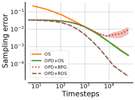
(b) With initial data

Figure 1: Sampling error (kl) curves of data collection in the GridWorld domain. Each strategy is followed to collect data with $2^{13}\overline{T}$ steps, and all results are averaged over $200$ trials with shading indicating one standard error intervals. Figures 1(a) and 1(b) show the sampling error curves of data collection without and with initial data, respectively. Axes in these figures are log-scaled.

We first run experiments in a setting without initial data, in which all data is collected from scratch. Letting $\overline{T}$ denote the average length of a trajectory, in each domain, we collect a total of $2^{13}\overline{T}$ environment steps with each method and compute metrics every $2^{1},2^{2},...,2^{13}$ trajectories. Note that we specify the number of environment steps rather than number of trajectories in our empirical results. For Bandit $\overline{T}=1$, for GridWorld $\overline{T}=7.43$, CartPole $\overline{T}=48.48$, and for CartPoleContinuous $\overline{T}=49.56$. The hyper-parameter settings for all experiments are presented in Appendix E.

We first verify that ros reduces sampling error compared to on-policy sampling. We measure sampling error with the kl-divergence (kl) between ${\pi_{e}}$ and a parametric maximum likelihood estimate of ${\pi_{D}}$ from the observe data. In Appendix D, we give a complete definition of the measure as well as an alternative measure that leads to qualitatively similar results. Due to space constraints, we only show this result for the GridWorld domain (Figure 1(a)); results for other domains are qualitatively the same and can be found in Appendix D.1. Figure 1(a) shows that with ros sampling error decreases faster than os. Unsurprisingly, bpg increases sampling error as it is an off-policy method which adapts the behavior policy away from ${\pi_{e}}$. These results answer our first empirical question and confirm our theoretical claim that non-i.i.d. off-policy sampling can cause the empirical distribution of data to converge to the expected on-policy distribution faster.

Ultimately, this paper focuses on reducing sampling error for lower mse policy evaluation. Figure 2 shows that ros lowers mse compared to both os and bpg across all domains. These results address our second empirical question and support the claim that reducing sampling error decreases the mse of the Monte Carlo estimator for policy evaluation.

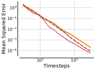
(a) Bandit

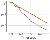
(b) GridWorld

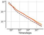
(c) CartPole

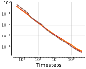
(d) CartPoleContinuous

Figure 2: Mean squared error (mse) of policy evaluation in the without initial data setting. Policy evaluation is conducted on the data collected from each strategy, and these curves show the mse of the estimates (lower is better). The vertical axis gives mse and the horizontal axis is the amount of environment steps taken (both are log-scaled). Shading indicates one standard error.

6.2 Policy Evaluation with Initial Data

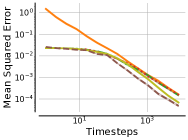
(a) Bandit

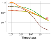
(b) GridWorld

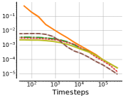
(c) CartPole

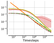
(d) CartPoleContinuous

Figure 3: Mean squared error (mse) of policy evaluation in the with initial data setting. Policy evaluation is conducted on the data collected from each strategy and a small set of initial data collected off-policy. Axes and confidence intervals are the same as in Figure 2.

Our next set of experiments considers a setting with initial data, in which a set of $100$ trajectories are already available and we wish to use these trajectories in our policy value estimate. These trajectories are collected via i.i.d. off-policy sampling with a behavior policy that is slightly different than ${\pi_{e}}$. This setting is intended to represent a setting where ${\pi_{e}}$ has just been updated from an older policy and we would like to still use the off-policy data already collected from the older policy combined with the data to be collected. In addition to the off-policy data (opd), we collect an additional $2^{13}\overline{T}$ steps of environment interaction with each method. We do not count the initial 100 trajectories towards the total collected data.

For ros, we use the opd to initialize $\nabla_{\boldsymbol{\theta}}{\mathcal{L}}$. We expect to see that ros will collect data to combine with the opd such that the aggregate data set looks as if it had been collected with ${\pi_{e}}$ to begin with. We compare ros to the following baseline methods. (opd + os)-mc collects additional data with os and uses the Monte Carlo estimator with the total data-set. (opd + os)-(wis + mc) uses weighted importance sampling (wis) to compute an estimate from the opd combines the wis estimate with a Monte Carlo estimate using on-policy data. (opd + bpg)-ois collects additional data with bpg and uses ordinary importance sampling as the estimator with all data. Finally, (os - mc) replaces the 100 initial trajectories with trajectories from os, then collects the remaining data with os and uses the Monte Carlo estimator. In the case of (os - mc), the 100 initial trajectories are counted towards the total data collected.

Figure 1(b) shows that sampling error decreases fastest for ros as the additional data is collected. For policy evaluation, we show mse for varying amounts of data in Figure 3 and provide numerical values for the final mse in Appendix F. We observe that the initial data provides an immediate reduction in mse at the expense of injecting bias into the estimates. (opd+os)-mc struggles to reduce this bias while (opd+ros)-mc is able to through data collection. Overall, this result highlights that ros can collect additional data that reduces sampling error in the aggregate data set and produce lower mse estimates compared to other data collection methods. Intuitively, os requires many more samples to dilute the bias brought on by using opd in the Monte Carlo estimator, while ros is able to correct the empirical off-policy distribution to the expected on-policy distribution and use the Monte Carlo estimator without any off-policy corrections.

The comparison to os-mc demonstrates the potential of ros for correcting an off-policy empirical distribution to the expected on-policy distribution. As noted above, os-mc has 100 fewer trajectories than the other baselines. However – even when including the initial 100 off-policy trajectories in the data total for all methods – ros eventually obtains lower mse compared to os-mc. In this sense, ros has taken an initially biased dataset and collected the right trajectories to make it look as-if the evaluation policy had collected all trajectories in the first place.

6.3 Sensitivity Study

Finally, we evaluate the sensitivity of ros to hyper-parameter, environment, and policy settings. ros requires setting a step size, $\alpha$, which controls how much ros updates the behavior policy away from ${\pi_{e}}$. We show mse curves for ros with different step size $\alpha$ on GridWorld and CartPole in Figures 4 ($\alpha=0$ corresponds to os). Figure 4(a) shows that, in GridWorld, ros with any tested step-size produces lower mse policy evaluation than os for any data set size. As it collects more data, ros with larger $\alpha$ enables lower mse because the norm of $\nabla_{\boldsymbol{\theta}}{\mathcal{L}}$ decreases as sampling error decreases, and thus a larger $\alpha$ is required to make significant updates. A larger $\alpha$ value is also in line with our theoretical results which prescribe $\alpha\rightarrow\infty$. However, in CartPole, (Figure 4(b)), ros with the largest tested $\alpha$ (1000) diverges and the second largest ($\alpha=100$) requires many steps before it improves upon os. Thus, in domains with continuous state-spaces, more conservative $\alpha$ values may be preferred.

Our final set of experiments considers how the stochasticity of a domain and entropy of ${\pi_{e}}$ affect the relative improvement that ros offers. In this sub-section, we study these settings in the Bandit domain for its simplicty; similar experimental results in GridWorld can be found in Appendix H. We choose $\alpha=1000$ for the following experiments.

To study domain stochasticity, we first create variants of the Bandit environment by multiplying either the mean or scale of the reward distribution of each action by a varying factor. In each experimental trial, we use ros to collect $1000\overline{T}$ steps for the Monte Carlo estimator and compute the relative mse compared to the Monte Carlo estimator using os with the same number of steps. Figure 4(c) shows that as the factor on the mean increases, ros provides a greater reduction in mse as even small amounts of sampling error translate into large mse when the reward means are large. On the other hand, as the scale factor increases, the mse is dominated by reward noise and the relative benefit of reducing sampling error disappears.

We also evaluate the relative improvement of ros as a function of the entropy of ${\pi_{e}}$. For ${\pi_{e}}$, we use $\epsilon$-greedy policies which select the optimal action in a state with probability $1-\epsilon$ and otherwise select an action uniformly at random. Relative improvement in mse is shown in Figure 4(d). For all $\epsilon$, ros improves upon the mse of os. The improvement is generally larger for more stochastic ${\pi_{e}}$ when sampling error in action selection will be highest.

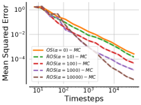
(a) GridWorld

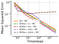
(b) CartPole

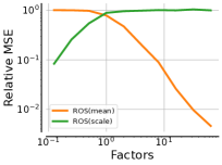
(c) Environment Noise

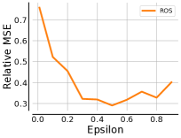
(d) Policy Noise

Figure 4: mse of ros with different step-size, $\alpha$ (4(a) and 4(b)). Relative improvement of ros in Bandit compared to os with different stochasticity in the environment (4(c)) and policy (4(d)). The relative MSE is computed as the MSE of ROS divided by the MSE of OS. Results in these figures are averaged over $500$ trials.

7 Discussion and Future Work

This work has shown that off-policy non-i.i.d. sampling can produce data sets that more closely approximate the on-policy data distribution than on-policy i.i.d. sampling. We considered the problem of policy evaluation and showed that more closely approximating the on-policy data distribution leads to more data efficient policy evaluation across several domains. As far as we know, ros is the first data collection method for policy evaluation that uses off-policy sampling to produce more closely on-policy data than the data produced by on-policy sampling.

While ros is a first step towards off-policy algorithms that produce data matching a target distribution, we highlight a few limitations of the algorithm and our study. In our view, the main limitations of the ros algorithm are the need to set a step-size parameter (in contrast to parameter-free on-policy sampling) and the need to update $\nabla_{\boldsymbol{\theta}}{\mathcal{L}}$ at each action step. For the former, future work should investigate robust methods for setting the step-size, particularly in settings where ${\pi_{\boldsymbol{\theta}}}$ generalizes across the state-space. For the latter limitation, a future study could consider only updating $\nabla_{\boldsymbol{\theta}}{\mathcal{L}}$ at the end of each episode instead of after each action choice (assuming more computation can be done between episodes). In terms of our study, for this paper we chose to study many different facets of ros on a suite of simpler domains (see the appendices for additional ablations and extensions); a future study should assess the scalability of ros with more complex function approximators. Finally, our theoretical results were conducted in the tabular setting; an important open question is at what rate ros converges when ${\pi_{\boldsymbol{\theta}}}$ uses a function approximator that must generalize across states. Beyond these minor technical limitations, our paper addresses fundamental research questions in rl and thus we do not see obvious negative societal impacts that are unique to this work in comparison to other work in rl and policy evaluation.

While we evaluated ros for policy evaluation, the long-term importance of this work may be in exploring the distinction between on-policy sampling and on-policy data. On-policy rl algorithms require on-policy data and our work suggests that adaptive off-policy sampling can produce on-policy data more efficiently than on-policy sampling. In the future, we wish to study these insights for on-policy policy improvement algorithms (e.g., policy gradient methods (Williams, 1992; Schulman et al., 2017)) and to extend our convergence results to non-tabular settings.

8 Conclusion

In this paper, we have introduced a novel data collection method for policy evaluation in reinforcement learning environments. Our method – Robust On-Policy Sampling (ros) – considers previously collected data when selecting actions to reduce sampling error in the entire collected data set. We show both in theory and in practice that data from ros converges faster to the on-policy data distribution compared to on-policy sampling. Empirically, we find that faster convergence to the on-policy data distributions lowers the mse of policy evaluation.

Checklist

1. For all authors…

   1. Do the main claims made in the abstract and introduction accurately reflect the paper’s contributions and scope? [Yes]

   2. Did you describe the limitations of your work? [Yes] See Section 7.

   3. Did you discuss any potential negative societal impacts of your work? [Yes] See Section 7.

   4. Have you read the ethics review guidelines and ensured that your paper conforms to them? [Yes]

2. If you are including theoretical results…

   1. Did you state the full set of assumptions of all theoretical results? [Yes] See Section 5.2 and Appendix B.

   2. Did you include complete proofs of all theoretical results? [Yes] See Appendices A and B.

3. If you ran experiments…

   1. Did you include the code, data, and instructions needed to reproduce the main experimental results (either in the supplemental material or as a Url)? [Yes] Included in supplementary material.

   2. Did you specify all the training details (e.g., data splits, hyperparameters, how they were chosen)? [Yes] See Section 6 and Appendices C.2 and E.

   3. Did you report error bars (e.g., with respect to the random seed after running experiments multiple times)? [Yes]

   4. Did you include the total amount of compute and the type of resources used (e.g., type of GPUs, internal cluster, or cloud provider)? [No] Experiments use rl domains and algorithms that can be ran on a typical personal computer. Minimal compute resources required to reproduce any experiment in the paper.

4. If you are using existing assets (e.g., code, data, models) or curating/releasing new assets…

   1. If your work uses existing assets, did you cite the creators? [Yes]

   2. Did you mention the license of the assets? [No]

   3. Did you include any new assets either in the supplemental material or as a Url? [No]

   4. Did you discuss whether and how consent was obtained from people whose data you’re using/curating? [N/A]

   5. Did you discuss whether the data you are using/curating contains personally identifiable information or offensive content? [N/A]

5. If you used crowdsourcing or conducted research with human subjects…

   1. Did you include the full text of instructions given to participants and screenshots, if applicable? [N/A]

   2. Did you describe any potential participant risks, with links to Institutional Review Board (IRB) approvals, if applicable? [N/A]

   3. Did you include the estimated hourly wage paid to participants and the total amount spent on participant compensation? [N/A]

Appendix A Proof of Proposition 1

In this appendix we prove Proposition 1 from Section 4.

See 1

Proof.

In the following, we use $\textbf{E}_{\pi_{e}}[\cdot]$ as shorthand for $\textbf{E}[\cdot|D\sim{\pi_{e}}]$. Let $\hat{v}_{1}\coloneqq\frac{1}{n_{{\cal D}_{1}}}\sum_{i=1}^{n_{{\cal D}_{1}}}g(h_{i})=\operatorname{MC}({\cal D}_{1})$.

$$\textbf{E}_{\pi_{e}}\biggl{[}\operatorname{MC}({\cal D}_{1}\cup D_{2})\biggr{]} =\textbf{E}_{\pi_{e}}\left[\frac{1}{n}\sum_{i=1}^{n_{{\cal D}_{1}}}g(h_{i})+\frac{1}{n}\sum_{i=1}^{n_{{{D}}_{2}}}g(H_{i})\right]$$ (5)

$$=\textbf{E}_{\pi_{e}}\left[\frac{1}{n}\sum_{i=1}^{n_{{\cal D}_{1}}}g(h_{i})\right]+\textbf{E}_{\pi_{e}}\left[\frac{1}{n}\sum_{i=1}^{n_{{{D}}_{2}}}g(H_{i})\right]$$ (6)

$$\overset{(a)}{=}\frac{1}{n}\frac{n_{{\cal D}_{1}}}{n_{{\cal D}_{1}}}\sum_{i=1}^{n_{{\cal D}_{1}}}g(h_{i})+\textbf{E}_{\pi_{e}}\left[\frac{1}{n}\frac{n_{{{D}}_{2}}}{n_{{{D}}_{2}}}\sum_{i=1}^{n_{{{D}}_{2}}}g(H_{i})\right]$$ (7)

$$\overset{(b)}{=}\frac{n_{{\cal D}_{1}}}{n}\hat{v}_{1}+\frac{n_{{{D}}_{2}}}{n}\textbf{E}_{\pi_{e}}\left[\underbrace{\frac{1}{n_{{{D}}_{2}}}\sum_{i=1}^{n_{{{D}}_{2}}}g(H_{i})}_{\operatorname{MC}(D_{2})}\right]$$ (8)

$$\overset{(c)}{=}\frac{n_{{\cal D}_{1}}}{n}\hat{v}_{1}+\frac{n_{{{D}}_{2}}}{n}v({\pi_{e}})$$ (9)

$$\overset{}{=}\frac{n_{{\cal D}_{1}}}{n}(\hat{v}_{1}-v({\pi_{e}}))+\frac{n_{{{D}}_{2}}}{n}v({\pi_{e}})+\frac{n_{{\cal D}_{1}}}{n}v({\pi_{e}})$$ (10)

$$\overset{}{=}\frac{n_{{\cal D}_{1}}}{n}(\hat{v}_{1}-v({\pi_{e}}))+v({\pi_{e}})$$ (11)

where (a) uses the fact that no random variables appear inside the first expectation, (b) uses the definition of $\hat{v}$, and (c) uses the fact that $\operatorname{MC}(D_{2})$ is an unbiased estimator of $v({\pi_{e}})$. The proposition follows by observing that equation 11 is equal to $v({\pi_{e}})$ if and only if $n_{{\cal D}_{1}}=0$ (i.e., ${\cal D}_{1}=\emptyset$) or if $\hat{v}=v({\pi_{e}})$.

Note that the latter case in which the data-conditioned Monte Carlo estimator is unbiased only occurs when the Monte Carlo estimate only using ${\cal D}_{1}$ has non-zero error. If $g(H)$ has non-zero variance under on-policy sampling then the probability that $\operatorname{MC}({\cal D}_{1})$ is exactly equal to $v({\pi_{e}})$ with a finite-size $D_{2}$ is low.

∎

Appendix B Proofs of ROS Properties

Before giving the proofs for Theorems 1 and 2 we re-state our key assumption. See 2

We next derive two lemmas that will be used in the proofs of our theorems.

Lemma 1.

Let $S_{m}(a)$ denote the number of times that action $a$ was taken after visiting a particular state, $s$, $m$ times in ${\cal D}$ and let $k\coloneqq|\mathcal{A}|$. Under Assumption 2 and ros collection of ${\cal D}$, we have that:

$$\sup_{a\in\mathcal{A}}|S_{m}(a)-m{\pi_{e}}(a|s)|\leq k-1.$$ (12)

Proof.

We first formally show that Assumption 2 implies that ros always taking the most under-sampled action at each time-step. Because we only consider a single state, we suppress dependencies on the state in this proof, e.g., we write ${\pi_{e}}(a)$ instead of ${\pi_{e}}(a|s)$ and $\theta_{a}$ instead of $\theta_{s,a}$ for the softmax parameters. We have ${\mathcal{L}}({\pi_{\boldsymbol{\theta}}})=\sum_{a}S_{m}(a)\theta_{a}-m\log(\sum_{b\in\mathcal{A}}e^{\theta_{b}})$ and $\nabla_{\theta_{a}}{\mathcal{L}}({\pi_{\boldsymbol{\theta}}})|_{{\pi_{\boldsymbol{\theta}}}={\pi_{e}}}=S_{m}(a)(1-{\pi_{e}}(a))-{\pi_{e}}(a)(m-S_{m}(a))=S_{m}(a)-m{\pi_{e}}(a)$, which is exactly the number of times that action $a$ was over-sampled. The softmax parameter for action $a$ after the ros update is given by:

$$\theta_{a}^{\prime}={\theta_{e,a}}-\alpha(S_{m}(a)-m{\pi_{e}}(a))$$

where $\theta_{e,a}$ is the softmax parameter for action $a$ under the evaluation policy. Taking the limit as $\alpha\rightarrow\infty$, we see that the $\theta_{e,a}$ term is dominated by the $\alpha(S_{m}(a)-{\pi_{e}}(a)m)$ term. Thus the parameter for each action is:

$$\theta_{a}^{\prime}=\alpha((m{\pi_{e}}(a)-S_{m}(a)).$$

Interpreting $\alpha$ as the inverse of the softmax temperature, we can see that $\alpha\rightarrow\infty$ corresponds to a softmax temperature $\rightarrow 0$ which in turn corresponds to a hard max over the $(m{\pi_{e}}(a)-S_{m}(a))$ values. Thus, the updated behavior policy puts all probability mass on the action for which ${\pi_{e}}(a)m-S_{m}(a)$ is largest. Hence we select the most under-sampled action if we take $\alpha\rightarrow\infty$ in Algorithm 1.

Now we show that under ros action selection that the amount of over- or under-sampling is bounded. First, we observe that,

$$\sum_{a\in\mathcal{A}}(S_{m}(i)-m{\pi_{e}}(i))=m-m=0,$$

and we claim that,

$$S_{m}(a)-m{\pi_{e}}(a)\leq 1$$

for any $a\in\mathcal{A}$. We prove this claim by contradiction. Assume not: $S_{m}(j)-m{\pi_{e}}(j)>1$ for some $j\in\mathcal{A}$. Let $X_{m}(j)\coloneqq 1$ if action $j$ was taken at step $m$ and $0$ otherwise. If $X_{m}(j)=1$, we have that:

$$S_{m}(j)-m{\pi_{e}}(i) >1\implies$$

$$S_{m-1}(j)+1-(m-1){\pi_{e}}(j)-{\pi_{e}}(j) >1\implies$$

$$S_{m-1}(j)-(m-1){\pi_{e}}(j) >1-1+{\pi_{e}}(j)>0.$$

However, this results in a contradiction since we have that action $j$ was over-sampled at the previous step but action $j$ would not be selected by ros if it was over-sampled. So, in order for $S_{m}(j)-m{\pi_{e}}(j)>1$, we must have that $X_{m}(j)=0$. Combining the fact that $X_{m}(j)=0$ with our assumption that $S_{m}(j)-m{\pi_{e}}(j)>1$ tells us that:

$$S_{m}(j)-m{\pi_{e}}(j)>1$$

$$\overset{(a)}{\implies} S_{m-1}(j)-m{\pi_{e}}(j)>1$$

$$\implies S_{m-1}(j)-(m-1){\pi_{e}}(j)>1$$

where (a) is because $S_{m-1}(j)$ must be equal to $S_{m}(j)$ if $X_{m}(j)=0$. By the same logic we get that $X_{m-1}(j)=x_{m-2}(j)=\cdots=X_{1}(j)=0$ which implies that $S_{1}(j)-{\pi_{e}}(j)=0-{\pi_{e}}>1$ which is a contradiction. Thus, we conclude that $S_{m}(j)-m{\pi_{e}}(j)\leq 1$ for any $j$, i.e., any action can be over-sampled by at most 1. Combining this conclusion with the observation that $\sum_{a\in\mathcal{A}}S_{m}(a)-m{\pi_{e}}(a)=m-m=0$ tells us that any action can be under-sampled by at most $k-1$. Thus, the absolute difference $|S_{m}(a)-m{\pi_{e}}(a)|$ is at most $k-1$ for any action $a\in\mathcal{A}$ which completes the proof.

∎

Lemma 2.

Let $s$ be a state that we visit $m$ times. Under ros sampling, we have $\forall a\in\mathcal{A}$ that:

$$\lim_{m\rightarrow\infty}\pi_{D}(a|s)={\pi_{e}}(a|s).$$

Proof.

The proof follows from Lemma 12. As in the proof of Lemma 12, we suppress the dependency on $s$ in our notation since we are only concerned with a fixed state. Using the notation from the proof of Lemma 12, we have that $\pi_{D}(a)=\frac{S_{m}(a)}{m}$.

$$|S_{m}(a)-m{\pi_{e}}(a)|\leq k-1$$

$$\implies \frac{|S_{m}(a)-m{\pi_{e}}(a)|}{m}\leq\frac{k-1}{m}$$

$$\implies \lim_{m\rightarrow\infty}\frac{|S_{m}(a)-m{\pi_{e}}(a)|}{m}\leq\lim_{m\rightarrow\infty}\frac{k-1}{m}$$

$$\implies \lim_{m\rightarrow\infty}|\pi_{D}(a)-{\pi_{e}}(a)|\leq 0$$

$$\implies \lim_{m\rightarrow\infty}|\pi_{D}(a)-{\pi_{e}}(a)|=0$$

$$\implies \lim_{m\rightarrow\infty}\pi_{D}(a)={\pi_{e}}(a).$$

∎

See 1

Proof.

The proof is by induction. For the base case, note that $d^{0}_{\pi}(s)=d_{0}(s)$ and thus $\lim_{n\rightarrow\infty}d^{0}_{n}(s)=d^{0}_{\pi}(s)$ $\forall s$ with probability $1$ by the strong law of large numbers.

For the induction step, we assume $\lim_{n\rightarrow\infty}d^{t}_{n}(s)=d^{t}_{\pi}(s)$ $\forall s$ with probability $1$ for some episode step $t<{l}$. We want to show that this implies that $\lim_{n\rightarrow\infty}d^{t+1}_{n}(s)=d^{t+1}_{\pi}(s)$ with probability $1$ for all $s$. Let $P_{n}$ denote the empirical state transition function, i.e., $P_{n}(s^{\prime}|s,a)\coloneqq\frac{c_{n}(s,a,s^{\prime})}{c_{n}(s,a)}$ where $c_{n}(s,a,s^{\prime})$ is the number of times that $(s,a,s^{\prime})$ occurred in $D$ and similarly for $c_{n}(s,a)$. Note that $d^{t+1}_{n}(s)=\sum_{\tilde{s}}\sum_{a}d^{t}_{n}(\tilde{s})\pi_{D}(a|\tilde{s})P_{n}(s|\tilde{s},a)$ and $d^{t+1}_{\pi}(s)=\sum_{\tilde{s}}\sum_{a}d^{t}_{\pi}(\tilde{s})\pi(a|\tilde{s})P(s|\tilde{s},a)$. The former claim follows as a consequence of the finite-horizon MDP setting in which the state implicitly must depend on the current time-step. In this setting $P_{n}(s^{\prime}|s,a)$ and ${\pi_{D}}(a|s)$ are only computed with samples from a particular time-step (or pair of subsequent time-steps in the case of $P_{n}$). Then we have that:

$$\lim_{n\rightarrow\infty}d^{t+1}_{n}(s)= \lim_{n\rightarrow\infty}\sum_{\tilde{s}}\sum_{a}d^{t}_{n}(\tilde{s})\pi_{D}(a|\tilde{s})P_{n}(s|\tilde{s},a)$$

$$= \sum_{\tilde{s}}\sum_{a}\lim_{n\rightarrow\infty}d^{t}_{n}(\tilde{s})\pi_{D}(a|\tilde{s})P_{n}(s|\tilde{s},a)$$

$$= \sum_{\tilde{s}}\sum_{a}\lim_{n\rightarrow\infty}d^{t}_{n}(\tilde{s})\cdot\lim_{n\rightarrow\infty}\pi_{D}(a|\tilde{s})\cdot\lim_{n\rightarrow\infty}P_{n}(s|\tilde{s},a)$$

$$= \sum_{\tilde{s}}\sum_{a}\lim_{n\rightarrow\infty}d^{t}_{n}(\tilde{s})\cdot\lim_{n\rightarrow\infty}\pi_{D}(a|\tilde{s})\cdot\lim_{n\rightarrow\infty}P_{n}(s|\tilde{s},a)$$

$$\overset{(a)}{=} \sum_{\tilde{s}}\sum_{a}d^{t}_{\pi}(\tilde{s})\pi(a|\tilde{s})P(s|\tilde{s},a)$$

$$= d^{t+1}_{\pi}(s)$$

where (a) follows from the induction hypothesis, Lemma 2, and $\lim_{n\rightarrow\infty}P_{n}(s^{\prime}|s,a)=P(s^{\prime}|s,a)$ follows from the strong law of large numbers. This completes the proof.

∎

See 2

Proof.

This proof has two parts. Since we only consider a particular state, we suppress the state-dependency in policies throughout this proof, i.e., we write $\pi(a)$ instead of $\pi(a|s)$. The on-policy sampling rate is adapted from Theorem 1 of Mardia et al. [2019] which implies that, the KL-divergence between the empirical distribution of a discrete distribution and that discrete distribution itself is $O_{p}(\frac{1}{m})$. In our case, ${\pi_{e}}$ is the discrete distribution and $\pi_{D}$ is the empirical distribution. Then we have from Mardia et al. [2019] that $2mD_{\mathtt{KL}}({\pi_{D}}||{\pi_{e}})\xrightarrow[]{d}\chi_{k-1}^{2}$ where $k$ is the number of actions. So we have that $D_{KL}({\pi_{D}}||{\pi_{e}})=O_{p}(\frac{1}{m})$ from Lemma 5.3 of Alexanderian [2009] since convergence in distribution implies bounded in probability.

Second, we obtain the ros rate. Define the vectors ${{\tilde{\pi}}_{e}}\coloneqq({\pi_{e}}(1),\cdots,{\pi_{e}}(k-1))$ and ${{\tilde{\pi}}_{D}}\coloneqq({\pi_{D}}(1),\cdots,{\pi_{D}}(k-1))$. We write the KL-divergence between ${\pi_{e}}$ and $\pi_{D}$ as a function of these two vectors:

$$D_{KL}({{\tilde{\pi}}_{D}}||{{\tilde{\pi}}_{e}})=\sum_{i=1}^{k-1}{{\tilde{\pi}}_{D}}(i)\log(\frac{{{\tilde{\pi}}_{D}}(i)}{{{\tilde{\pi}}_{e}}(i)})+(1-\sum_{j=1}^{k-1}{{\tilde{\pi}}_{D}}(j))\log(\frac{1-\sum_{j=1}^{k-1}{{\tilde{\pi}}_{D}}(j)}{1-\sum_{j=1}^{k-1}{{\tilde{\pi}}_{e}}(j)}).$$

Let $\mathbf{g}$ denote the gradient of $D_{KL}({{\tilde{\pi}}_{D}}||{{\tilde{\pi}}_{e}})$ with respect to $\tilde{\pi}_{D}$, evaluated at point $\tilde{\pi}_{e}$ and $\mathbf{H}$ denotes the Hessian matrix of $D_{KL}({\pi_{D}}||{\pi_{e}})$ evaluated at point $\tilde{\pi}_{e}$. Clearly, $\mathbf{g}=\mathbf{0}$ because setting ${\pi_{D}}$ to ${\pi_{e}}$ will minimize $D_{\mathtt{KL}}(\pi_{D}||{\pi_{e}})$. We take the Hessian from Mardia et al. [2019]:

$$\mathbf{H}(i,j)=\begin{cases}\frac{1}{{\pi_{e}}(k)}&i\neq j\\ \frac{1}{{\pi_{e}}(i)}+\frac{1}{{\pi_{e}}(k)}&i=j\end{cases}$$

Alternatively, we can write $\mathbf{H}=\frac{1}{{\pi_{e}}(k)}\mathbf{1}\mathbf{1}^{\top}+\mathtt{diag}({{\tilde{\pi}}^{-1}}_{e})$ where $\mathtt{diag}({\tilde{\pi}_{e}}^{-1})$ is the $(k-1\times k-1)$ matrix with $\frac{1}{\tilde{\pi}_{e}}$ on its diagonal. Using a Taylor Series expansion for $D_{\mathtt{KL}}$, we have:

$$m^{2}D_{\mathtt{KL}}({\pi_{D}}||{\pi_{e}})=m^{2}D_{\mathtt{KL}}({\pi_{e}}||{\pi_{e}})+m^{2}\mathbf{g}^{T}(\tilde{\pi}_{D}-\tilde{\pi}_{e})+\underbrace{\frac{1}{2}m(\tilde{\pi}_{D}-\tilde{\pi}_{e})^{T}\mathbf{H}m(\tilde{\pi}_{D}-\tilde{\pi}_{e})}_{\text{Quadratic Term}}+Q_{m}$$

where $Q_{m}$ consists of the higher order terms. Note that since $D_{\mathtt{KL}}({\pi_{e}}||{\pi_{e}})=0$, the first two terms are both 0 so we only need to bound the quadratic term and higher terms. By Lemma 12 every component of $m(\tilde{\pi}_{D}-\tilde{\pi}_{e})$ is bounded by $k-1$, so the quadratic term is bounded by $\frac{1}{2}\sum_{i,j}\mathbf{H}(i,j)(k-1)^{2}$, which is of order $O(1)$ since $\mathbf{H}$ is a constant when evaluated at ${\tilde{\pi}}_{e}$. The higher order terms $Q_{m}$ contain higher powers of $({\tilde{\pi}}_{D}-{\tilde{\pi}}_{e})$ multiplied by $m^{2}$. Using Lemma 12, we can bound all components of any $m(\tilde{\pi}_{D}-\tilde{\pi}_{e})$ by $k-1$ to replace each $m$ with a constant (trivially, all components of $(\tilde{\pi}_{D}-\tilde{\pi}_{e})$ can also be bounded by $k-1$) and higher-order derivatives of $D_{\mathtt{KL}}$ evaluated at ${\pi_{e}}$ are also constant with respect to $m$. Thus higher order terms are also $O(1)$ which gives us that $m^{2}D_{\mathtt{KL}}(\pi_{D}||{\pi_{e}})=O(1)$ and thus that $D_{\mathtt{KL}}(\pi_{D}||{\pi_{e}})=O(\frac{1}{m^{2}})$. Deterministic convergence to zero implies probabilistic convergence and thus, under ros action selection, $D_{\mathtt{KL}}(\pi_{D}||{\pi_{e}})=O_{p}(\frac{1}{m^{2}})$. ∎

See 3

Proof.

First, we introduce some additional notation. We define $\mu_{n}^{t}(s,a)\coloneqq\frac{n_{t}(s,a)}{n}$ as the empirical distribution of a state-action pair at time $t$, where $n_{t}(s,a)$ is the number of times that state $s$ and action $a$ occur jointly at time $t$ across trajectories in ${\cal D}$. Let $\mu_{\pi_{e}}^{t}(s,a)$ be the probability of state $s$ and action $a$ occurring jointly at time $t$ while following ${\pi_{e}}$. Note that $\mu_{n}^{t}(s,a)=d_{n}^{t}(s){\pi_{D}}(a|s)$ and $\mu_{\pi_{e}}^{t}(s,a)=d_{\pi_{e}}^{t}(s){\pi_{e}}(a|s)$. Finally, we define $n(s_{0},a_{0},\dots,s_{{l}-1},a_{{l}-1})$ as the number of times that state-action trajectory $s_{0},a_{0},\dots,s_{{l}-1},a_{{l}-1}$ occurs in ${\cal D}$.

Observe that the Monte Carlo estimate can be re-written as:

$$\operatorname{MC}({{D}})= \frac{1}{n}\sum_{i=1}^{n}\sum_{t=0}^{{l}-1}\gamma^{t}R(s_{i,t},a_{i,t})$$

$$= \frac{1}{n}\sum_{s_{0}}\sum_{a_{0}}\cdots\sum_{s_{{l}-1}}\sum_{a_{{l}-1}}n(s_{0},a_{0},\dots,s_{{l}-1},a_{{l}-1})\sum_{t=0}^{{l}-1}\gamma^{t}R(s_{t},a_{t})$$

$$= \frac{1}{n}\sum_{t=0}^{{l}-1}\gamma^{t}\sum_{s_{0}}\sum_{a_{0}}\cdots\sum_{s_{{l}-1}}\sum_{a_{{l}-1}}n(s_{0},a_{0},\dots,s_{{l}-1},a_{{l}-1})R(s_{t},a_{t})$$

$$= \frac{1}{n}\sum_{t=0}^{{l}-1}\gamma^{t}\sum_{s}\sum_{a}n_{t}(s,a)R(s,a)$$

$$= \sum_{t=0}^{{l}-1}\gamma^{t}\sum_{s}\sum_{a}\mu_{n}^{t}(s,a)R(s,a).$$

Similarly, the true value of the evaluation policy can be re-written in terms of the state-action distribution at each time step under policy ${\pi_{e}}$:

$$v({\pi_{e}})= \sum_{h}\Pr(h|{\pi_{e}})\sum_{t=0}^{{l}-1}\gamma^{t}R(s_{h,t},a_{h,t})$$

$$= \sum_{s_{0}}\sum_{a_{0}}\cdots\sum_{s_{{l}-1}}\sum_{a_{{l}-1}}\underbrace{d_{0}(s_{0}){\pi_{e}}(a_{0}|s_{0})\prod_{i=1}^{{l}-1}{\pi_{e}}(a_{i}|s_{i})P(s_{i}|s_{i-1},a_{i-1})}_{=\Pr(h=(s_{0},a_{0},\dots,s_{{l}-1},a_{{l}-1})|{\pi_{e}})}\sum_{t=0}^{{l}-1}\gamma^{t}R(s_{t},a_{t})$$

$$= \sum_{t=0}^{{l}-1}\gamma^{t}\sum_{s_{0}}\sum_{a_{0}}\cdots\sum_{s_{{l}-1}}\sum_{a_{{l}-1}}d_{0}(s_{0}){\pi_{e}}(a_{0}|s_{0})\cdots P(s_{{l}-1}|s_{{l}-2},a_{{l}-2})R(s_{t},a_{t})$$

$$= \sum_{t=0}^{{l}-1}\gamma^{t}\sum_{s}\sum_{a}\mu_{\pi_{e}}^{t}(s,a)R(s,a)$$

Now, we use these alternative formulations to bound the squared error between the true value and the Monte Carlo estimate computed with a fixed data-set ${{D}}$.

$$(v({\pi_{e}})-\operatorname{MC}({{D}}))^{2} =\left(\sum_{t=0}^{{l}-1}\gamma^{t}\sum_{s}\sum_{a}R(s,a)(\mu_{n}^{t}(s,a)-\mu_{\pi_{e}}^{t}(s,a))\right)^{2}$$

$$\overset{(a)}{\leq}\sum_{t=0}^{{l}-1}\gamma^{2t}\sum_{s}\sum_{a}\left(R(s,a)(\mu_{n}^{t}(s,a)-\mu_{\pi_{e}}^{t}(s,a))\right)^{2}$$

$$\overset{(b)}{\leq}\sum_{t=0}^{{l}-1}\gamma^{2t}R_{\mathtt{max}}^{2}\sum_{s}\sum_{a}\left(\mu_{n}^{t}(s,a)-\mu_{\pi_{e}}^{t}(s,a)\right)^{2}$$

$$\overset{(c)}{\leq}\sum_{t=0}^{{l}-1}\gamma^{2t}R_{\mathtt{max}}^{2}\sum_{s}\sum_{a}\left|\mu_{n}^{t}(s,a)-\mu_{\pi_{e}}^{t}(s,a)\right|$$

$$\overset{(d)}{\leq}\sum_{t=0}^{{l}-1}\gamma^{2t}R_{\mathtt{max}}^{2}\sqrt{2D_{\mathtt{KL}}(\mu_{n}^{t}||\mu_{\pi_{e}}^{t})}$$

where (a) uses Jensen’s inequality, (b) replaces $R(s,a)$ with the constant $r_{\mathtt{max}}$, (c) notes that $-1\geq\mu_{n}^{t}(s,a)-\mu_{\pi_{e}}^{t}(s,a)\leq 1$ so $|\mu_{n}^{t}(s,a)-\mu_{\pi_{e}}^{t}(s,a)|\geq(\mu_{n}^{t}(s,a)-\mu_{\pi_{e}}^{t}(s,a))^{2}$, and (d) uses Pinsker’s inequality. All that remains is to use the definition of the KL-divergence and properties of logarithms and expectations to obtain the final form of the bound:

$$\sum_{t=0}^{{l}-1}\gamma^{2t}R_{\mathtt{max}}^{2}\sqrt{2D_{\mathtt{KL}}(\mu_{n}^{t}||\mu_{\pi_{e}}^{t})} =\sum_{t=0}^{{l}-1}\gamma^{2t}R_{\mathtt{max}}^{2}\sqrt{2E_{S\sim d_{n}^{t},A\sim\pi_{{D}}}[\log\frac{d_{n}^{t}(S){\pi_{D}}(A|S)}{d_{\pi_{e}}^{t}(S){\pi_{e}}(A|S)}]}$$

$$=\sum_{t=0}^{{l}-1}\gamma^{2t}R_{\mathtt{max}}^{2}\sqrt{2E_{S\sim d_{n}^{t},A\sim\pi_{{D}}}[\log\frac{d_{n}^{t}(S)}{d_{\pi_{e}}^{t}(S)}+\log\frac{{\pi_{D}}(A|S)}{{\pi_{e}}(A|S)}]}$$

$$=\sum_{t=0}^{{l}-1}\gamma^{2t}R_{\mathtt{max}}^{2}\sqrt{2D_{\mathtt{KL}}(d_{n}^{t}||d_{\pi_{e}}^{t})+2\mathbf{E}_{S\sim d_{n}^{t}}[D_{\mathtt{KL}}(\pi_{D}(\cdot|S)||{\pi_{e}}(\cdot|S)]}.$$

∎

Appendix C Experiment Domains

This appendix provides additional details on our experimental set-up.

C.1 Extended Domain Descriptions

This section describes the domains used in our empirical evaluation. Figure 5 illustrates each domain.

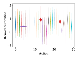
(a) Bandit

(b) GridWorld

(c) CartPole

Figure 5: Experimental Domains. Figure 5(a) shows the distribution of rewards from each action in a $30$-armed bandit problem, with black dots indicating the mean rewards and shading indicating the scale of the distribution. Figure 5(b) shows a $4\times 4$ GridWorld with the agent starting from the bottom-left corner and the goal state in the top-right corner. Figure 5(c) shows the CartPole environment in which the goal is to keep the pole from falling over. ContinuousCartPole is the same as CartPole except with a modified action space.

Our first domain, Bandit, is a 30-armed bandit problem modelled after the 10-armed bandit in Sutton and Barto [1998, Chapter 2]. This domain has a single state, 30 actions, and episodes terminate after the first action is taken. The reward following each action is normally distributed with a randomly generated mean and scale parameter. The reward distribution parameters are sampled from a uniform distribution on $[0,1]$ at the start of each experimental trial.

Our second domain, GridWorld, is a discrete state and action domain that has been used in prior policy evaluation research (e.g., [Thomas and Brunskill, 2016, Farajtabar et al., 2018]). The domain (shown in Figure 5(b)) has $4\times 4$ states. The agent starts from $(0,0)$ and has the action space {left, right, up, down}. The reward is $-1$ in all non-terminal states except $(1,1)$ where the reward is $-10$ and $(1,3)$ where the reward is $+1$. The agent receives $+10$ in terminal state $(3,3)$. The maximum number of steps is $100$ and $\gamma=1$ in this domain.

Our last two domains are based on the CartPole problem from OpenAI Gym [Brockman et al., 2016]. In CartPole, the agent tries to balance a pole, mounted on a cart, by moving the cart left and right. States are given as vectors that describe the cart position and velocity and pole angle and angular velocity. Our third domain is the standard variant in which the agent controls the cart by choosing either a constant leftward force of $-1$, no force, or a constant rightward force of $+1$. Our fourth domain is a continuous control variant in which the agent can control the exact force ranging from $-1$ to $1$. In either case, the agent receives a reward of $+1$ for each time-step until termination when the pole falls or the cart moves out of bounds. The maximum number of steps is $200$ and $\gamma=0.99$ in this domain.

C.2 Creation of Pre-trained Evaluation Policy

Each domain requires creation of an evaluation policy to serve as ${\pi_{e}}$. In the three domains with a discrete action space we use softmax policies of the form:

$${\pi_{\boldsymbol{\theta}}}(a|s)\propto\frac{e^{w_{a}^{\top}\mathbf{\phi}(s)}}{\sum_{b\in\mathcal{A}}e^{w_{b}^{\top}\mathbf{\phi}(s)}}$$ (13)

where $\mathbf{\phi}$ is a one-hot encoding operator for domains with discrete state space (Bandit and GridWorld) and a feed-forward neural network for continuous state spaces (CartPole). For ContinuousCartPole,

$${\pi_{\boldsymbol{\theta}}}(a|s)\coloneqq\mathcal{N}\left(a;\mathbf{w}_{\mu}^{\top}\mathbf{\phi}(s),\left(\mathbf{w}_{\sigma}^{\top}\mathbf{\phi}(s)\right)^{2}\right),$$ (14)

where $\mathbf{\phi}$ is a function of the state given by a feed-forward neural network. The policy parameters, ${\boldsymbol{\theta}}$, denote all policy parameters. For Bandit and GridWorld, this is just the vectors $\mathbf{w_{a}}$ and for CartPole and ContinuousCartPole, ${\boldsymbol{\theta}}$ also includes the neural network weights and biases. When $\mathbf{\phi}$ is a neural network, it is constructed with one batch normalization layer as the first layer, followed by two hidden layers, both of which have 64 hidden states and use ReLU as the activation function. We use PyTorch for neural network implementations [Paszke et al., 2019] and NumPy for linear algebra computations [Harris et al., 2020].

For all domains, we use REINFORCE [Williams, 1992] to train the policy model, and choose a policy snapshot during training as the evaluation policy, which has higher returns than the uniformly random policy, but is still far from convergence. To obtain $v({\pi_{e}})$, we use on-policy sampling to collect $10^{6}$ trajectories and compute the Monte Carlo estimate of $v({\pi_{e}})$.

C.3 Off-policy Data for With Initial Data Experiments

To create an initial data set of slightly off-policy data for each domain, we create the behavior policy ${\pi_{b}}$ based on the evaluation policy $\pi_{e}$. For domains with discrete action space, the off-policy behavior policy is built as:

$${\pi_{b}}(a|s)=(1-\delta){\pi_{e}}(a|s)+\delta\frac{1}{\lvert\mathcal{A}\rvert}$$

where $\delta\in(0,1]$ controls the probability of randomly choosing an action from the action space, and otherwise sampling an action from the evaluation policy ${\pi_{e}}$. For ContinuousCartPole, the behavior policy is built as:

$${\pi_{b}}(a|s)=\mathcal{N}\left(a;\mu_{e}(s),\left(\left(1+\delta\right)\sigma_{e}(s)\right)^{2}\right)$$

where $\mu_{e}(s)$ and $\sigma_{e}(s)$ are the output mean and standard deviation of the evaluation policy $\pi_{e}$ in state $s$, and $\delta$ (for $\delta>0$) increases the standard deviation. In all domains, we use $\delta=0.1$ and collect 100 trajectories to create the initial off-policy data set.

Appendix D Measuring Sampling Error

One of our central claims is that ros reduces sampling error and reducing sampling error corresponds to a reduction in mse for policy evaluation. To evaluate this claim, we must define a metric for measuring sampling error. In this appendix, we describe two possible metrics and demonstrate how these metrics change as os and ros collect data for policy evaluation.

D.1 KL-divergence of Data Collection

Our first metric (also used in the main paper), is to measure sampling error in the collected data $D$ by using KL-divergence of the empirical policy $\pi_{D}$ and the evaluation policy $\pi_{e}$. The KL-divergence between $\pi_{D}$ and ${\pi_{e}}$ in a particular state $s$ is defined as:

$$D_{\mathtt{KL}}(\pi_{D},{\pi_{e}})\coloneqq\textbf{E}\biggl{[}\log\frac{\pi_{D}(A|s)}{{\pi_{e}}(A|s)}\biggm{|}A\sim\pi_{D}\biggr{]}.$$

To obtain an explicit representation of $\pi_{D}$, we use a parametric estimate by maximizing the log-likelihood function over a parametric policy class. Specifically, we use:

$$\hat{{\boldsymbol{\theta}}}=\arg\max_{{\boldsymbol{\theta}}^{\prime}}\sum_{(s,a)\in{\cal D}_{1}}\log\pi_{{\boldsymbol{\theta}}^{\prime}}(a|s)$$

for a policy class parameterized by ${\boldsymbol{\theta}}$. We then use $\pi_{\hat{{\boldsymbol{\theta}}}}$ in place of $\pi_{D}$ when computing the KL-divergence. Our final sampling error metric for a data set ${\cal D}_{1}$ is:

$$D_{\mathtt{KL}}({\pi_{e}},D)\coloneqq\sum_{(s,a)\in{\cal D}_{1}}\log\pi_{\hat{{\boldsymbol{\theta}}^{\prime}}}(a|s)-\log{\pi_{e}}(a|s).$$

The sampling error curves of data collection without and with initial data are shown in Figure 6 and 7, respectively. We observe from these experiments that ros can collect data with lower sampling error than os and bpg.

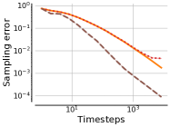
(a) Bandit

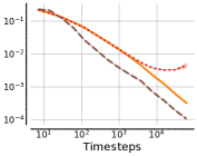
(b) GridWorld

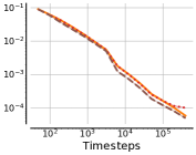
(c) CartPole

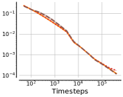
(d) ContinuousCartPole

Figure 6: Sampling error (KL) of data collection without initial data. Each strategy is followed to collect data with $2^{13}\overline{T}$ steps, and all results are averaged over $200$ trials with shading indicating one standard error intervals. Axes in these figures are log-scaled.

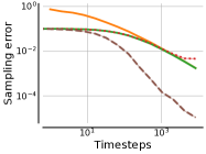
(a) Bandit

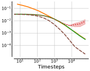
(b) GridWorld

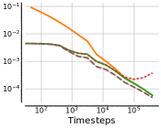
(c) CartPole

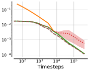
(d) ContinuousCartPole

Figure 7: Sampling error (KL) of data collection with initial data. Steps, axes, trials and intervals are the same as Figure 6.

D.2 l1-Norm of the Log-likelihood Gradient

In this section, we propose an alternative sampling error measure based on the norm of the log-likelihood gradient evaluated at ${\pi_{e}}$. If ${\pi_{e}}$ is the maximum likelihood policy under ${\cal D}$ then the norm of the gradient evaluated at ${\boldsymbol{\theta}}_{e}$ will be zero when sampling error is zero. A non-zero norm indicates the parameters must change from ${\boldsymbol{\theta}}_{e}$ to maximize the log-likelihood under the observed data. We show empirically that this measure of sampling error roughly corresponds to using the KL-divergence by computing the gradient norm of log-likelihood with respect to the data collection without and with initial data, shown in Figure 8 and 9, respectively. These curves are generally consistent with their corresponding sampling error curves in Appendix D.1.

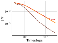
(a) Bandit

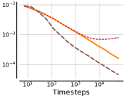
(b) GridWorld

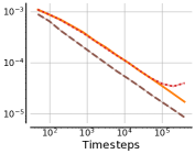
(c) CartPole

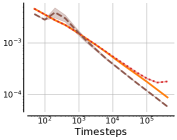
(d) ContinuousCartPole

Figure 8: Log-likelihood gradient of the data collection without initial data. Steps, axes, trials and intervals are the same as Figure 6.

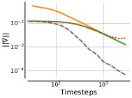
(a) Bandit

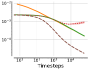
(b) GridWorld

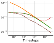
(c) CartPole

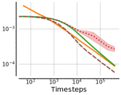
(d) ContinuousCartPole

Figure 9: Log-likelihood gradient of the data collection with initial data. Steps, axes, trials and intervals are the same as Figure 6.

Appendix E Hyper-parameter Configurations

This appendix gives the hyper-parameter settings for the policy evaluation experiments. Settings for the without initial data experiments are given in Table 1 and settings for the with initial data experiments are given in Table 2. For bpg, $k$ denotes the batch-size and $\alpha$ the step-size.

Domain	bpg - $k$	bpg - $\alpha$	ros - $\alpha$
Bandit	10	0.01	10000.0
GridWorld	10	0.01	1000.0
CartPole	10	5e-05	10.0
CartPoleContinuous	10	1e-06	0.1

Table 1: Hyper-parameters for experiments without initial data.

Domain	bpg - $k$	bpg - $\alpha$	ros - $\alpha$
Bandit	10	0.01	10000.0
GridWorld	10	0.01	10000.0
CartPole	10	5e-05	10.0
CartPoleContinuous	10	1e-06	0.1

Table 2: Hyper-parameters for experiments with initial data.

Appendix F Numerical Results of Policy Evaluation with Initial Data

This appendix provides the numerical final values for the mse of policy evaluation with each data collection method. Table 3 gives these values for the without initial data experiments and Table 4 gives these values for the with initial data experiments. These tables provide the numerical value corresponding to the final mse value for each method-domain pair shown in Figures 2 and 3.

Policy Evaluation	Bandit	GridWorld	CartPole	CartPoleContinuous
OS - MC	2.06e-04 $\pm$ 2.12e-05	2.68e-04 $\pm$ 2.42e-05	2.61e-05 $\pm$ 2.40e-06	4.44e-05 $\pm$ 4.01e-06
bpg - OIS	9.52e-05 $\pm$ 8.83e-06	2.81e-04 $\pm$ 2.63e-05	1.20e-05 $\pm$ 1.11e-06	3.62e-05 $\pm$ 3.54e-06
ros - MC	6.17e-05 $\pm$ 5.77e-06	1.36e-05 $\pm$ 1.33e-06	1.01e-05 $\pm$ 9.79e-07	3.29e-05 $\pm$ 3.01e-06

Table 3: Final mse of policy evaluation without initial data. These results give the mse for policy evaluation at the end of data collection, averaged over 200 trials $\pm$ one standard error.

Policy Evaluation	Bandit	GridWorld	CartPole	CartPoleContinuous
OS - MC	1.62e-04 $\pm$ 1.45e-05	2.68e-04 $\pm$ 2.42e-05	2.61e-05 $\pm$ 2.40e-06	4.44e-05 $\pm$ 4.01e-06
(OPD + OS) - MC	1.48e-04 $\pm$ 1.41e-05	2.80e-04 $\pm$ 2.82e-05	2.69e-05 $\pm$ 2.70e-06	4.27e-05 $\pm$ 3.72e-06
(OPD + OS) - (WIS + MC)	1.56e-04 $\pm$ 1.70e-05	2.65e-04 $\pm$ 2.40e-05	2.59e-05 $\pm$ 2.51e-06	6.02e-05 $\pm$ 8.51e-06
(OPD + bpg) - OIS	6.86e-05 $\pm$ 7.46e-06	9.20e-04 $\pm$ 6.27e-04	1.52e-05 $\pm$ 1.53e-06	1.12e-03 $\pm$ 9.58e-04
(OPD + ros) - MC	4.78e-05 $\pm$ 4.81e-06	2.35e-06 $\pm$ 2.42e-07	9.60e-06 $\pm$ 9.35e-07	3.27e-05 $\pm$ 3.21e-06

Table 4: Final mse of policy evaluation with initial data. These results give the mse for policy evaluation at the end of data collection, averaged over 200 trials $\pm$ one standard error.

Appendix G Median and Inter-quartile Range of Policy Evaluation

In this appendix, we present the computed median and interquartile range for the squared error of policy evaluation both with and without initial data across all four domains. In the main paper we present the mean squared error and standard error as is typical in the policy evaluation literature. Here, we include the median and interquartile ranges as they are more robust statistics. We give these results for completeness; qualitatively, they leave the conclusions from the main paper unchanged.

Figure 10 shows the median and interquartile ranges for policy evaluation without initial data. Figure 11 gives the same for policy evaluation with initial data. From these figures, we can observe that all data collection methords have a similar inter-quartile range and ros lowers the median of the squared error compared to os.

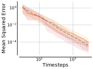
(a) Bandit

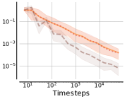
(b) GridWorld

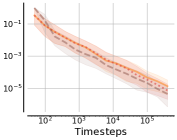
(c) CartPole

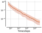
(d) ContinuousCartPole

Figure 10: Median and inter-quartile range of squared error (SE) of policy evaluation without initial data. The lines in these figures denote the median of squared error over 200 trials, and the shading indicates the interquartile range. Axes in these figures are log-scaled.

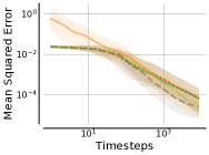
(a) Bandit

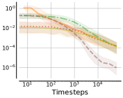
(b) GridWorld

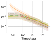
(c) CartPole

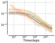
(d) ContinuousCartPole

Figure 11: Median and inter-quartile range of squared error (SE) of policy evaluation with initial data. Axes, trials and intervals are the same as Figure 10.

Appendix H Environment and Policy Sensitivity in GridWorld

In the main paper, we evaluated the relative mse of ros compared to os in the Bandit environment under different settings of the reward scale and variance and the stochasticity of ${\pi_{e}}$. In this appendix, we repeat the same study in the GridWorld environment. The original GridWorld domain has fixed rewards for each state. We vary these by either 1) multiplying by a fixed factor (referred to as the mean factor) or 2) replacing the deterministic reward with a reward sampled uniformly from $[-f_{\text{scale}},f_{\text{scale}}]$ where $f_{\text{scale}}$ determines the reward variance. We then follow os or ros ($\alpha=1000$) to collect $1000$ trajectories, and perform Monte Carlo estimation. The relative mses between os and ros are shown in Figure 12(a). Results show an identical trend to the Bandit environment: a larger reward scale increases the amount of improvement because small amounts of sampling error can lead to larger amounts of error; larger reward variance decreases the amount of improvement because the mse becomes dominated by variance in the reward.

We also create different evaluation policies using $\epsilon$-greedy policies with $\epsilon$ ranging from $0$ to $1$. We then perform the same policy evaluation as above and compute the relative mses, shown in Figure 12(b). As with the Bandit domain, we see that greater entropy in ${\pi_{e}}$ generally leads to a wider margin of improvement between ros and os.

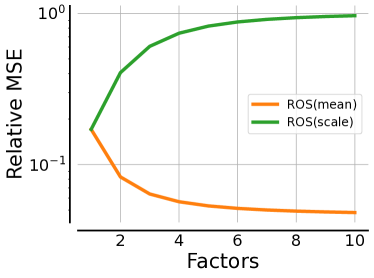
(a) Environment Settings

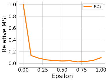
(b) Policy Settings

Figure 12: Improvement of ros compared to os with different settings in GridWorld. Axes and trials are the same as Figure 4.

Appendix I Mean Squared Error of Policy Evaluation with WRIS and FQE

This appendix presents preliminary results on combining ros with estimators specifically designed for the off-policy setting instead of the Monte Carlo estimator. Specifically, we used weighted regression importance sampling (wris) [Hanna et al., 2021] and fitted q-evaluation (fqe) [Le et al., 2019]. We study these estimators in the without initial data setting and show their mse with varying amounts of data. Figure 13 shows the mse of different data collection methods for wris across the different domains. Figure 14 shows the same except with fqe as the estimator.

We observe in tabular domains that os cannot obtain the same level mse as ros, even with the help of wris, which is designed to correct sampling error during the value estimation stage. This shows the importance of reducing sampling error during the data collection stage. The same pattern can also be observed when using fqe. In non-tabular domains, the performances of off-policy evaluation methods with different data collection methods are very similar. However, wris usually requires larger sizes of data to make accurate estimation, and can only achieve similar mse as ros when collecting a large amount of data. When using fqe in non-tabular domains, data from ros can generally enable lower mse than os, although this improvement is very small.

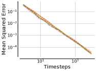
(a) Bandit

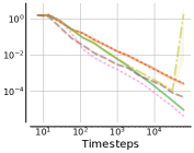
(b) GridWorld

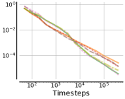
(c) CartPole

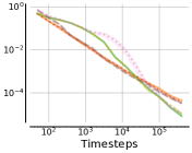
(d) ContinuousCartPole

Figure 13: mse of WRIS without initial data. Steps, axes, trials and intervals are the same as Figure 2.

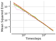
(a) Bandit

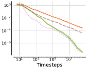
(b) GridWorld

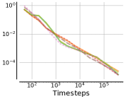
(c) CartPole

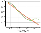
(d) ContinuousCartPole

Figure 14: mse of FQE without initial data. Steps, axes, trials and intervals are the same as Figure 2.

References

- Agarwal et al. [2022] Alekh Agarwal, Nan Jiang, Sham M. Kakade, and Wen Sun. Reinforcement learning: Theory and algorithms. 2022.
- Alexanderian [2009] Alen Alexanderian. Some notes on asymptotic theory in probability. Notes. University of Maryland, 2009.
- Arnold et al. [2022] Sébastien M. R. Arnold, Pierre L’Ecuyer, Liyu Chen, Yi-fan Chen, and Fei Sha. Policy learning and evaluation with randomized quasi-monte carlo. In International Conference on Artificial Intelligence and Statistics, 2022.
- Bouchard et al. [2016] Guillaume Bouchard, Théo Trouillon, Julien Perez, and Adrien Gaidon. Online learning to sample. arXiv preprint arXiv:1506.09016, 2016.
- Brockman et al. [2016] Greg Brockman, Vicki Cheung, Ludwig Pettersson, Jonas Schneider, John Schulman, Jie Tang, and Wojciech Zaremba. OpenAI Gym. arXiv preprint arXiv:1606.01540, 2016.
- Ciosek and Whiteson [2017] Kamil Ciosek and Shimon Whiteson. OFFER: Off-environment reinforcement learning. In AAAI Conference on Artificial Intelligence, 2017.
- Farajtabar et al. [2018] Mehrdad Farajtabar, Yinlam Chow, and Mohammad Ghavamzadeh. More robust doubly robust off-policy evaluation. In International Conference on Machine Learning, 2018.
- Frank et al. [2008] Jordan Frank, Shie Mannor, and Doina Precup. Reinforcement learning in the presence of rare events. In International Conference on Machine Learning, 2008.
- Hanna et al. [2017] Josiah P. Hanna, Philip S. Thomas, Peter Stone, and Scott Niekum. Data-efficient policy evaluation through behavior policy search. In International Conference on Machine Learning, 2017.
- Hanna et al. [2021] Josiah P. Hanna, Scott Niekum, and Peter Stone. Importance Sampling in Reinforcement Learning with an Estimated Behavior Policy. Machine Learning, 110(6):1267–1317, May 2021.
- Harris et al. [2020] Charles R. Harris, K. Jarrod Millman, Stéfan J. van der Walt, Ralf Gommers, Pauli Virtanen, David Cournapeau, Eric Wieser, Julian Taylor, Sebastian Berg, Nathaniel J. Smith, Robert Kern, Matti Picus, Stephan Hoyer, Marten H. van Kerkwijk, Matthew Brett, Allan Haldane, Jaime Fernández del Río, Mark Wiebe, Pearu Peterson, Pierre Gérard-Marchant, Kevin Sheppard, Tyler Reddy, Warren Weckesser, Hameer Abbasi, Christoph Gohlke, and Travis E. Oliphant. Array programming with NumPy. Nature, 585(7825):357–362, 2020.
- Jiang and Li [2016] Nan Jiang and Lihong Li. Doubly robust off-policy evaluation for reinforcement learning. In International Conference on Machine Learning, 2016.
- Konyushova et al. [2021] Ksenia Konyushova, Yutian Chen, Thomas Paine, Caglar Gulcehre, Cosmin Paduraru, Daniel J. Mankowitz, Misha Denil, and Nando de Freitas. Active offline policy selection. In Advances in Neural Information Processing Systems, 2021.
- Le et al. [2019] Hoang Le, Cameron Voloshin, and Yisong Yue. Batch policy learning under constraints. In International Conference on Machine Learning, 2019.
- Li et al. [2015] Lihong Li, Rémi Munos, and Csaba Szepesvári. Toward minimax off-policy value estimation. In International Conference on Artificial Intelligence and Statistics, 2015.
- Mardia et al. [2019] Jay Mardia, Jiantao Jiao, Ervin Tánczos, Robert D Nowak, and Tsachy Weissman. Concentration inequalities for the empirical distribution of discrete distributions: beyond the method of types. Information and Inference: A Journal of the IMA, 9(4):813–850, 2019.
- Mukherjee et al. [2022] Subhojyoti Mukherjee, Josiah P. Hanna, and Robert Nowak. ReVar: Strengthening Policy Evaluation via Reduced Variance Sampling. In International Conference on Uncertainty in Artificial Intelligence (UAI), August 2022.
- Narita et al. [2019] Yusuke Narita, Shota Yasui, and Kohei Yata. Efficient counterfactual learning from bandit feedback. In AAAI Conference on Artificial Intelligence, 2019.
- O’Hagan [1987] Anthony O’Hagan. Monte carlo is fundamentally unsound. The Statistician, pages 247–249, 1987.
- Oosterhuis and de Rijke [2020] Harrie Oosterhuis and Maarten de Rijke. Taking the counterfactual online: Efficient and unbiased online evaluation for ranking. In International Conference on Theory of Information Retrieval, 2020.
- Ostrovski et al. [2017] Georg Ostrovski, Marc G. Bellemare, Aäron Oord, and Rémi Munos. Count-based exploration with neural density models. In International conference on machine learning, 2017.
- Paszke et al. [2019] Adam Paszke, Sam Gross, Francisco Massa, Adam Lerer, James Bradbury, Gregory Chanan, Trevor Killeen, Zeming Lin, Natalia Gimelshein, Luca Antiga, Alban Desmaison, Andreas Kopf, Edward Yang, Zachary DeVito, Martin Raison, Alykhan Tejani, Sasank Chilamkurthy, Benoit Steiner, Lu Fang, Junjie Bai, and Soumith Chintala. PyTorch: An imperative style, high-performance deep learning library. In Advances in Neural Information Processing Systems. 2019.
- Pavse et al. [2020] Brahma S. Pavse, Ishan Durugkar, Josiah P. Hanna, and Peter Stone. Reducing sampling error in batch temporal difference learning. In International Conference on Machine Learning, 2020.
- Puterman [2014] Martin L. Puterman. Markov decision processes: discrete stochastic dynamic programming. John Wiley & Sons, 2014.
- Rasmussen and Ghahramani [2003] Carl Edward Rasmussen and Zoubin Ghahramani. Bayesian monte carlo. In Advances in Neural Information Processing Systems, 2003.
- Schäfer et al. [2022] Lukas Schäfer, Filippos Christianos, Josiah P. Hanna, and Stefano V. Albrecht. Decoupled reinforcement learning to stabilise intrinsically-motivated exploration. In International Conference on Autonomous Agents and Multiagent Systems, 2022.
- Schulman et al. [2017] John Schulman, Filip Wolski, Prafulla Dhariwal, Alec Radford, and Oleg Klimov. Proximal policy optimization algorithms. arXiv preprint arXiv:1707.06347, 2017.
- Sen and Singer [1993] Pranab K. Sen and Julio M. Singer. Large Sample Methods in Statistics: An Introduction with Applications. Chapman & Hall, 1993.
- Sutton and Barto [1998] Richard S. Sutton and Andrew G. Barto. Reinforcement Learning: An Introduction. MIT Press, 1998.
- Tang et al. [2017] Haoran Tang, Rein Houthooft, Davis Foote, Adam Stooke, Xi Chen, Yan Duan, John Schulman, Filip De Turck, and Pieter Abbeel. # exploration: A study of count-based exploration for deep reinforcement learning. In Advances in neural information processing systems, 2017.
- Thomas and Brunskill [2016] Philip S. Thomas and Emma Brunskill. Data-efficient off-policy policy evaluation for reinforcement learning. In International Conference on Machine Learning, 2016.
- Tucker and Joachims [2022] Aaron David Tucker and Thorsten Joachims. Variance-optimal augmentation logging for counterfactual evaluation in contextual bandits. arXiv preprint arXiv:2202.01721, 2022.
- Williams [1992] Ronald J. Williams. Simple statistical gradient-following algorithms for connectionist reinforcement learning. Machine learning, 8(3):229–256, 1992.
- Zinkevich et al. [2006] Martin Zinkevich, Michael Bowling, Nolan Bard, Morgan Kan, and Darse Billings. Optimal unbiased estimators for evaluating agent performance. In AAAI Conference on Artificial Intelligence, 2006.