Periodic and chaotic dynamics in a map-based neuron model

Abstract

[Abstract] Map-based neuron models are an important tool in modelling neural dynamics and sometimes can be considered as an alternative to usually computationally costlier models based on continuous or hybrid dynamical systems. However, due to their discrete nature, rigorous mathematical analysis might be challenging. We study a discrete model of neuronal dynamics introduced by Chialvo [Chaos, Solitons & Fractals 5, 1995, 461–479]. In particular, we show that its reduced one-dimensional version can be treated as an independent simple model of neural activity where the input and the fixed value of the recovery variable are parameters. This one-dimensional model still displays very rich and varied dynamics. Using the fact that the map whose iterates define voltage dynamics is S-unimodal, we describe in detail both the periodic behaviour and the occurrence of different notions of chaos, indicating corresponding regions in parameter space. Our study is also complemented by a bifurcation analysis of the mentioned dynamical model.

Introduction

In the last decades many different types of neuron models have been developed, including conductance-based models (with the pioneering example of the experimentally derived Hodgkin-Huxley model ¹ or Morris-Lecar model ²) and other models based on continuous dynamical systems, i.e., differential equations (e.g. FitzHugh-Nagumo model ^{3, 4}), models based on discrete dynamical systems, i.e., iterates of functions (so-called map-based models), up to hybrid models which combine ordinary differential equations (accounting for input integration) with discrete events (resetting mechanism accounting for action potential), see e.g. ^{5, 6, 7, 8}.

In this paper we study the following map-based neuron model, introduced in ⁹:

$$x_{n+1} =f(x_{n},y_{n})=x_{n}^{2}\exp{(y_{n}-x_{n})}+k,$$ (1a)

$$y_{n+1} =g(x_{n},y_{n})=ay_{n}-bx_{n}+c.$$ (1b)

This model will be referred to as the 2D Chialvo model (or full Chialvo model). In the 2D Chialvo model (1a)–(1b) $x$ is a membrane voltage-potential (the most important dynamical variable in all the neuron models) and $y$ is so-called recovery variable. The time-constant $a\in(0,1)$, the activation-dependence $b\in(0,1)$ and the offset $c>0$ are the real parameters connected with the recovery process. In turn, $k\geq 0$ can be interpreted as an additive perturbation of the voltage. In our analysis, the 1-dimensional subsystem

$$x_{n+1}=f(x_{n},r)=x_{n}^{2}\exp{(r-x_{n})}+k,$$ (2)

where $r\in\mathbb{R}$ is a parameter, will be referred to as the 1D or reduced Chialvo model.

Other examples of map-based models are, among others, Cazelles-Courbage-Rabinovich model ¹⁰, different types of Rulkov models ^{11, 12, 13} or Courbage-Nekorkin-Vdovin model ¹⁴. In particular, the work of Zhong et al. ¹⁵ is devoted to the non-chaotic Rulkov-model ¹², where the analysis, similarly as in our case, firstly concerns bifurcations in the one-dimensional reduced model, i.e., fast subsystem describing the evolution of the membrane voltage, and shows that it produces fold and flip bifurcations. This subsystem also produces chaos as it is shown by numerical simulations. Different examples of map-based neuron models are discussed e.g. in review articles ^{16, 17} (see also references therein).

In this work we obtain rigorous characterization of chaos and co-dimension-one bifurcations of fixed points in the subsystem (2), relevant for the classification of bursting neurons. Before we start let us summarize the known results on Chialvo model and introduce notations. Obviously, the fixed points $(x_{f},y_{f})$ of the full model must satisfy

$$x_{f} =x_{f}^{2}\exp(y_{f}-x_{f})+k,$$

$$y_{f} =(c-bx_{f})/(1-a).$$

In particular, for $k=0$ the point $(x_{f_{0}},y_{f_{0}}):=(0,c/(1-a))$ is always a stable fixed point of the system as can be seen by calculating corresponding eigenvalues which are $0$ and $a$ (and $a<1$ by the assumption). Further, as Chialvo observed ⁹, when $b\ll a$, the initial part of the trajectory with initial condition $(x,y_{f_{0}})$ where $x\approx 0$ can be well described by the 1D Chialvo model (2) with $k=0$ and $r=y_{f_{0}}=c/(1-a)$. Therefore in this parameter regime, among others, the 1D subsystem gives the information about initial dynamics following the small perturbation of the resting state $x=0$ in the full model. A few other observations for $k>0$ (referring mainly to the situation where the system (1a)–(1b) has exactly one fixed point $(x_{f},y_{f})$) were made already in Chialvo’s work ⁹, including identification of some regions of bistability (coexistence of stable resting state and stable periodic oscillations) and regions of chaotic-like behaviour interspersed with subregions of periodic behaviour.

For more results on the full model, we also refer the reader to the more recent works ^{18, 19}. In particular, Jing et al. ¹⁸ studied analytically the existence and stability of the fixed points, conditions for existence of flip, fold and Hopf bifurcations and chaos in the sense of Marotto’s definition. Further, it numerically reports various period doubling bifurcations and routes to chaos, periodic windows in transient chaotic regions and strange chaotic and non-chaotic attractors, whereas the work of Wang and Cao ¹⁹ illustrates numerically the existence of interesting structures in parameter space.

As our work is mainly concerned with the 1-dimensional subsystem (2) we have only briefly described above the findings on the full 2D model. However, we go back to the analysis of the full model at the end of the paper. Let us also observe that for $0<\varepsilon=1-a=b=c\ll 1$, the system (1a)–(1b) can be seen as a slow-fast (discrete) system, i.e. the system of the form

$$x_{n+1} =\tilde{f}(x_{n},y_{n}),$$ (3a)

$$y_{n+1} =y_{n}+\varepsilon\tilde{g}(x_{n},y_{n}),$$ (3b)

where $\varepsilon\to 0$ is a small parameter. For this particular assumptions on parameters, the separation of timescales in the Chialvo model (1a)–(1b) is explicit. However, for many other choices of parameter values the timescale separation is not so explicit but still visible in simulations. In this case, the voltage variable $x$ and the recovery variable $y$, can be referred to as fast and slow variables, respectively. Consequently, while $x_{n}$ describes spiking behavior, $y_{n}$ acts as a slowly changing parameter (with time-scale variation $\varepsilon\ll 1$) that modulates the spiking dynamics.

Models of the form (3a)–(3b) are usually analized by firstly assuming that $\varepsilon=0$ and treating (3a) as a quazi-static approximation of (3a)–(3b) with parameter $y_{n}\equiv y$. If for some values of $y$ (3a) exhibits equilibrium dynamics (due to the existence of a stable fixed point) and for some other values it exhibits periodic dynamics (due to the existence of a stable periodic orbit), then bursting in the system (3a)–(3b) occurs because slowly varying $y_{n}$ acts as bifurcation parameter that makes the dynamics of $x$ switching between these two regimes (similar approach can be applied for ODE bursting systems, compare e.g. with ²⁰). Therefore bursting behaviour in the above neuron model is indeed directly connected with the types of bifurcations present in the fast system (3a) (correspondingly, in (1a) or (2)). According to this observation, in ²¹ the classification of bursting mappings was obtained, taking into account that there are only four possible co-dimension-1 bifurcations of a stable fixed point in maps (3a) that lead to its loss of stability or disappearance (fold, SNIC-saddle node on invariant circle bifurcation and supercritical and subcritical flip bifurcations) and only five co-dimension one bifurcations of a stable periodic orbit, which make the dynamics settle on a stable equilibrium afterwards (SNIC, homoclinic bifurcation, supercritical flip bifurcation, fold periodic orbit bifurcation and subcritical flip of periodic orbits bifurcation). The former bifurcations correspond to transition from resting to spiking frequently (i.e. the onset of bursting), the later ones to the transition back to resting and their combination defines the type of burster in a given neuron model. We also remark that classification of bursting types in ODEs neuron models was discussed e.g. in ²² and ²⁰ as well as in the recent article ²³ (see also review article ²⁴ and references therein).

It is also worth pointing out that, contrary to most of the 2D map based-models, the recovery variable $y$ in Chialvo model enters the voltage equation (1a) not in additive but in multiplicative way and changes the shape of the first return map $x_{n}\mapsto x_{n+1}=f(x_{n},y)$ of the $x$ variable in a complicated nonlinear way instead of just shifting the $x$-nullcline upward or downward. Therefore understanding how the map $f_{r,k}(x):=x^{2}\exp{(r-x)}+k$ depends not only on the additive parameter $k$ but also on the parameter $r$ is helpful for the analysis of the overall model. In fact $y$ variable in the Chialvo model can also be intended to represent fast, not slow dynamics (as already mentioned in the review article ¹⁷). When playing with the 2D model we have often observed that for many parameters configurations $y$ variable quickly stabilized at certain value $y_{s}$ while the voltage variable $x$ still evolved in an oscillatory way. In such a case types of voltage oscillations can be well explained by understanding the dynamics of the 1D model with corresponding value of parameter $r=y_{s}$ (we exemplify this in section 2.4).

The main aim of this paper is to study the 1D Chialvo model using the methods of one-dimensional dynamics. According to our best knowledge, it has never been pointed out that the map describing the membrane voltage evolution in the Chialvo model is an $S$-unimodal map and thereby there are no results on this model, which use the theory of $S$-unimodal maps. This basic observation that we make allows to draw relevant conclusions for this map, as well as, in some cases, for the whole model itself. Another example of the occurrence of unimodal maps in the context of neuron dynamics is the adaptation map of the bidimensional integrate-and-fire model ²⁵ (however, this unimodal map is given in a very implicit way and hardly ever exhibits negative Schwarzian derivative). In addition, it may be worth pointing out that various discrete systems similar to the 1D Chialvo model, for example the logistic family $Q(x)=\lambda x(1-x)$, the Ricker family $R(x)=\lambda x\exp(-\beta x)$ and the Hassell family $H(x)=\lambda x/(1+x)^{\beta}$, have been the subject of both theoretical and numerical intensive research study since the mid-1970s (see for instance ^{26, 27, 28, 29, 30}).

Let us also note that $f(z)=z^{2}\exp{(r-z)}+k$ (for the fixed complex values of parameters $r$ and $k$) can be seen as an example of a complex entire transcendental analytic function of finite type, i.e., having finite number of critical and asymptotic values. Since such maps exhibit, in general, different dynamical properties than polynomials, their complex dynamics (Julia and Fatou sets, etc.) has been studied extensively since the early 1980s (see ^{31, 32, 33} and the references given there). However, the approach presented in this paper is focused on one-dimensional methods and, in consequence, we do not make use of complex dynamics theory in our paper.

The organization of the paper is as follows. In Section 2 we examine the existence and stability of fixed points and corresponding bifurcations in the one-dimensional Chialvo model (2). Section 3 is devoted to the study of the dynamical core of the 1D Chialvo map. Further, in Section 4 we provide the description of periodic and chaotic behaviour of the model making use of the fact that (2) is given by an S-unimodal map. To ease our analysis we introduce basic concepts and definitions of the theory of S-unimodal maps in Section 1. Finally, concluding remarks are presented in Discussion section at the end of the paper.

1 Basic definitions

1.1 Unimodality and Schwarzian derivative

We say that an interval map $f\colon I\rightarrow I$ has negative Schwarzian derivative if $f$ is of class $C^{3}$ and

$$Sf(x):=\frac{f^{\prime\prime\prime}(x)}{f^{\prime}(x)}-\frac{3}{2}\left(\frac{f^{\prime\prime}(x)}{f^{\prime}(x)}\right)^{2}<0$$

for all $x\in I\setminus\left\{c\mid f^{\prime}(c)=0\right\}$. Points at which $f^{\prime}(c)=0$ are called critical points. The Schwarzian derivative was introduced in one-dimensional dynamics by D. Singer³⁴, but its origins go back to Hermann Schwarz and 19th century complex analysis.

A continuous interval map $f\colon I=\left[a,b\right]\to I$ is called unimodal if there is a unique maximum $c$ in the interior of $I$ such that $f$ is strictly increasing on $\left[a,c\right)$ and strictly decreasing on $\left(c,b\right]$. For simplicity, the term unimodal will also require that either $a$ is a fixed point with $b$ as its other preimage, or that $I=\left[f^{2}(c),f(c)\right]$. A unimodal map with negative Schwarzian derivative is called S-unimodal.

The itinerary of $x$ under $f$ is the sequence $s(x)=(s_{0}s_{1}s_{2}\dotsc)$ where

$$s_{j}=\begin{cases}0&\text{if $f^{j}(x)<c$},\\ 1&\text{if $f^{j}(x)>c$},\\ C&\text{if $f^{j}(x)=c$}.\end{cases}$$

The kneading sequence $K(f)$ of $f$ is the itinerary of $f(c)$, i.e., $K(f)=s\big{(}f(c)\big{)}$.

1.2 Bifurcations

Let $x_{0}$ be a fixed point for $f$. The point $x_{0}$ is called hyperbolic if $\left\lvert f^{\prime}(x_{0})\right\rvert\neq 1$. The number $\mu=f^{\prime}(x_{0})$ is called the multiplier of the fixed point. Consider a one-dimensional discrete dynamical system depending on a parameter $a$

$$x\mapsto f(x,a),\quad x\in\mathbb{R},\;a\in\mathbb{R},$$ (4)

where $f$ is smooth with respect to both $x$ and $a$. Let $x_{0}$ be a hyperbolic fixed point of the system. While the parameter $a$ varies, the hyperbolicity condition can be violated. The bifurcation associated with the appearance of the multiplier $\mu=1$ is called fold or tangent and with the appearance of the multiplier $\mu=-1$ flip or period-doubling. Alternatively a fold bifurcation is called a saddle-node bifurcation. Let us recall a classical result concerning these bifurcations (³⁵ Th. 4.1 and 4.3).

Theorem 1.1.

Suppose that a one-dimensional system (4) with smooth $f$, has at $a=0$ the fixed point $x_{0}=0$. Let $\mu:=\frac{\partial f}{\partial x}(0,0)$. If $\mu=1$ and the following conditions are satisfied:

1. $\frac{\partial^{2}f}{\partial x^{2}}(0,0)\neq 0$,

2. $\frac{\partial f}{\partial a}(0,0)\neq 0$,

then a fold bifurcation occurs at the fixed point $x_{0}=0$ for the bifurcation value $a=0$.

On the other hand, if $\mu=-1$ and the following conditions are satisfied:

1. $\frac{1}{2}\Big{(}\frac{\partial^{2}f}{\partial x^{2}}(0,0)\Big{)}^{2}+\frac{1}{3}\frac{\partial^{3}f}{\partial x^{3}}(0,0)\neq 0$,

2. $\frac{\partial^{2}f}{\partial x\partial a}(0,0)\neq 0$,

then a flip bifurcation occurs at the fixed point $x_{0}=0$ for the bifurcation value $a=0$.

Remark 1.2.

Based on the nonlinear stability of the fixed point at the bifurcation point we distinguish two cases for the flip bifurcation. If the quantity

$$\mathcal{Q}f(0,0):=\frac{1}{2}\Big{(}\frac{\partial^{2}f}{\partial x^{2}}(0,0)\Big{)}^{2}+\frac{1}{3}\frac{\partial^{3}f}{\partial x^{3}}(0,0)$$

in the (B.1) condition above is positive, the fixed point loses its stability at the bifurcation value and new stable $2$-periodic orbit emerges, in which case the flip bifurcation is called supercritical. Otherwise, i.e. when $\mathcal{Q}f(0,0)<0$, the fixed point turns unstable as it coalesces with an unstable $2$-periodic orbit and the bifurcation is called subritical.

1.3 Attractors

A set $\Gamma$ is called forward invariant if $f(\Gamma)=\Gamma$. The $\omega$-limit set (or forward limit set) of $x$ is defined as $\omega(x)=\bigcap_{n\in\mathbb{N}}\overline{\left\{f^{k}(x)\mid k>n\right\}}$, where $\overline{A}$ stands for the closure of $A$. Let $B(\Gamma)$ denote the basin of attraction of a forward invariant set $\Gamma$, that is, $B(\Gamma)=\{x\mid\omega(x)\subset\Gamma\}$. A forwards invariant set $\Omega$ is called a metric attractor if $B(\Omega)$ satisfies:

1. $B(\Omega)$ has positive Lebesgue measure;

2. if $\Omega^{\prime}$ is another forward invariant set, strictly contained in $\Omega$, then $B(\Omega)\setminus B(\Omega^{\prime})$ has positive measure.

We will need two well-known results concerning attractors for unimodal maps with negative Schwarzian derivative (for example ²⁹ Th. 4, Cor. 5 and Th. 6). Let $x$ be a periodic point of period $n$. Its periodic orbit is called neutral if $\left\lvert(f^{n})^{\prime}(x)\right\rvert=1$.

Theorem 1.3.

An S-unimodal map can have at most one periodic attractor, and it will attract the critical point. Moreover, each neutral periodic orbit is attracting.

By a periodic attractor in the above statement we obviously mean an attracting periodic orbit, i.e. a periodic orbit which is a forward-limit set for each point in some its neighbourhood.

Theorem 1.4.

Let $f\colon I\rightarrow I$ be an S-unimodal map with nonflat critical point. Then $f$ has a unique metric attractor $\Omega$, such that $w(x)=\Omega$ for almost all $x\in I$. The attractor $\Omega$ is of one of the following types: an attracting periodic orbit, a Cantor set of measure zero, a finite union of intervals with a dense orbit. In the first two cases, $\Omega=\omega(c)$.

The attractor described in (3) will be called an interval attractor for brevity.

2 Bifurcations in the Chialvo model

We start with the observation that will be crucial for our further analysis.

Proposition 2.1.

The map $f(x)=x^{2}\exp{(r-x)}+k$ has negative Schwarzian derivative for all $r,k\in\mathbb{R}$.

Proof 2.2.

By the definition of the Schwarzian derivative,

$$Sf(x)=-\frac{1}{2}\frac{x^{4}-8x^{3}+24x^{2}-24x+12}{(2x-x^{2})^{2}}=-\frac{1}{2}\frac{(x^{2}-4x+2)^{2}+4(x-1)^{2}+4}{(2x-x^{2})^{2}}.$$

This is obviously negative for all $x$ (even for $x$ equal to $0$ or $2$ we have $Sf(x)=-\infty$), which completes the proof.

Thus the function whose iterations define the reduced Chialvo model (2) is an S-unimodal map, when restricted to an appropriate invariant subinterval of $[0,\infty)$, as will be discussed in details in the next section. However, let us firstly examine bifurcations of fixed points of the map $f_{r,k}$, when $k\geq 0$ is fixed and $r$ acts as a bifurcation parameter.

We will discuss flip and fold bifurcations of fixed points for the reduced Chialvo model. Loosing stability of the fixed point and emergence of the stable periodic orbit in case of the flip bifurcation is relevant for the onset of bursting in the full 2D model. Let us also mention that other codimension-one bifurcations of fixed points, as well as bifurcations of periodic orbits responsible for the onset or termination of bursting in map-based models, are summarized in ²¹ (with examples of models and corresponding voltage-plots), which provides classification of one-dimensional and two-dimensional slow-fast bursting mappings with the implications for neuron’s computational abilities.

2.1 Flip bifurcation

Theorem 2.3 (flip bifurcation).

Let $k\geq 0$ be fixed. For $r_{0}=x_{0}-\ln\big{(}x_{0}(x_{0}-2)\big{)}$ (or equivalently $r_{0}=x_{0}+\ln\big{(}(x_{0}-k)/{x_{0}^{2}}\big{)}$) the 1D Chialvo map undergoes a supercritical flip bifurcation at the fixed point $x_{0}=(k+3+\sqrt{k^{2}-2k+9})/{2}$.

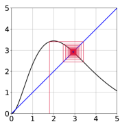
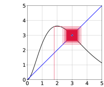
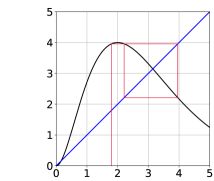
Figure 1: Flip bifurcation in the 1D Chialvo model with $r$ as a bifurcation parameter ($k=0$). Left: $r=1.85$. Center: $r=3-\ln{3}$ (bifurcation value). Right: $r=2$.

Proof 2.4.

Any fixed point $x_{0}$ of the map $f_{r,k}(x)=x^{2}\exp(r-x)+k$ must satisfy the fixed point condition $x_{0}=x_{0}^{2}\exp(r-x_{0})+k$. Simultaneously, the multiplier condition for the flip bifurcation gives

$$f^{\prime}_{r_{0},k}(x_{0})=x_{0}\exp(r_{0}-x_{0})(2-x_{0})=-1.$$

It follows that (when $k\geq 0$) the candidate $x_{0}$ for the flip bifurcation satisfies $x_{0}>\max\{2,k\}$ and $(x_{0}-k)(x_{0}-2)/x_{0}=1$. The last equation, regardless of the value of $k$, has always two roots $x_{0,1}=(k+3-\sqrt{k^{2}-2k+9})/{2}$ and $x_{0,2}=(k+3+\sqrt{k^{2}-2k+9})/{2}$. However, $x_{0,1}$ violates the condition that $x_{0}>k$. Thus $x_{0}=x_{0,2}$. The formula for the parameter value $r_{0}$ follows from the multiplier condition (or equivalently the fixed point condition) and the condition (B.2) of Theorem 1.1 can be easily verified as direct calculations give $\frac{\partial^{2}f}{\partial r\partial x}(x_{0},r_{0})=-1\neq 0$. Similarly, the negative value of the Schwarzian derivative immediately implies that the condition (B.1) is also satisfied, as $\mathcal{Q}f(x_{0},r_{0})=-Sf/{3}$, and the bifurcation is supercritical.

The flip bifurcation, for $k=0$, is numerically illustrated in Figure 1 with the help of the cobweb diagram.

2.2 Fold bifurcation

Theorem 2.5 (fold bifurcation).

Let $k\in[0,3-2\sqrt{2})$ be fixed. Then the 1D Chialvo model undergoes a fold bifurcation with $r$ as a bifurcation parameter. In particular, for $k=0$ and $r_{0}=1$ the map in (2) displays a fold bifurcation at the fixed point $x_{0}=1$. In turn, for fixed $0<k\leq 3-2\sqrt{2}$, there are two values of the bifurcation parameter, $r_{0,1}=x_{0,1}-\ln((2-x_{0,1})x_{0,1})$ and $r_{0,2}=x_{0,2}-\ln((2-x_{0,2})x_{0,2})$, with corresponding values of bifurcating fixed points given, respectively, as $x_{0,1}=(k+1-\sqrt{k^{2}-6k+1})/{2}$ and $x_{0,2}=(k+1+\sqrt{k^{2}-6k+1})/{2}$.

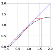
Figure 2: Fold bifurcation in the 1D Chialvo model with $r$ as a bifurcation parameter ($k=0$). Left: $r=0.92$. Center: $r=1$ (bifurcation value). Right: $r=1.25$.

Proof 2.6.

Assume $k=0$. From the fixed point condition $x^{2}\exp(r-x)=x$ and the multiplier condition $f^{\prime}(x)=x\exp(r-x)(2-x)=1$ we easily obtain that the only candidate for the bifurcation point and parameter value is a pair $(x_{0},r_{0})=(1,1)$. It is also immediate to verify that for these values the conditions (A.1) and (A.2) of Theorem 1.1 are satisfied.

For $k>0$ the situation is a bit more complicated. Firstly, the fixed point condition $x^{2}\exp(r-x)+k=x$ and the multiplier condition $\mu=1$ yield that the fold bifurcation is only possible for $k<2$ and the candidate $x_{0}$ for the fixed point undergoing bifurcation must satisfy $k<x_{0}<2$. Combining the multiplier condition with the fixed point condition gives $(2-x_{0})(x_{0}-k)/{x_{0}}=1$, or equivalently $x_{0}^{2}-(k+1)x_{0}+2k=0$. The discriminant of this equation $k^{2}-6k+1$ must be non-negative which leads to further restriction on admissible values of $k$, namely $k\leq 3-2\sqrt{2}$. Now, the above quadratic equation has the roots $x_{0,1}$ and $x_{0,2}$ as stated in the theorem, which both belong to the interval $(k,2)$. When $x_{0}=x_{0,1}$ or $x_{0}=x_{0,2}$ the corresponding values of the bifurcation parameter ($r_{0,1}$ and $r_{0,2}$) can be easily derived from the multiplier condition $x_{0}\exp(r-x_{0})(2-x_{0})=1$. We need to verify the conditions (A.1) and (A.2) at the points $(x_{0,1},r_{0,1})$ and $(x_{0,2},r_{0,2})$. The latter one can only be violated when $x_{0,1}=0$ or $x_{0,1}=k$ (correspondingly, $x_{0,2}=0$ or $x_{0,2}=k$). But these two cases have been excluded. As for (A.1), $\frac{\partial^{2}f}{\partial x^{2}}(x,r)=\exp(r-x)((x-2)^{2}-2)$ and thus direct calculations show that $\frac{\partial^{2}f}{\partial x^{2}}(x_{0},r_{0})=0$ (for $(x_{0},r_{0})\in\{(x_{0,1},r_{0,1}),(x_{0,2},r_{0,2})\}$) only for $k=3-2\sqrt{2}$. Hence the restriction $k<3-2\sqrt{2}$ in the theorem on the fold bifurcation (we notify that $k=3-2\sqrt{2}$ is the degenerate case when $x_{0,1}=x_{0,2}=2-\sqrt{2}$).

The fold bifurcation with respect to $r$ ($k=0$) is presented in Figure 2.

2.3 Bifurcations with respect to $k$

Let us consider now $k$ as a bifurcation parameter in the reduced Chialvo model. Since $\frac{\partial^{2}f}{\partial x\partial k}(x,k)=0$, the fundamental condition for the occurrence of a flip bifurcation is not satisfied here. However, the analysis of a fold bifurcation versus the parameter $k$ is still possible, which is discussed below.

Theorem 2.7 (fold bifurcation with respect to $k$).

Let $r>2-\sqrt{2}-\ln\big{(}2\sqrt{2}-2\big{)}$ be fixed. Then there is a unique point $x(r)$ and a unique parametr value $k^{*}$ such that $x(r)$ is the fixed point of the 1D Chialvo map in the interval $(0,2-\sqrt{2})$ for $k=k^{*}$ and $x(r)$ undergoes a fold bifurcation with respect to $k$ at the bifurcation value $k^{*}$. Moreover, the fixed point and the the bifurcation value are related by the equation

$$k^{*}=x(r)-\frac{x(r)}{2-x(r)}.$$

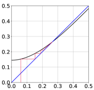
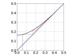
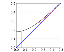
Figure 3: Fold bifurcation in the 1D Chialvo model with $k$ as a bifurcation parameter ($r=0.08$). Left: $k=0.151$. Center: $k=0.1627$ (numerical bifurcation value). Right: $k=0.18$.

Proof 2.8.

Observe that for $r>2-\sqrt{2}-\ln\big{(}2\sqrt{2}-2\big{)}$ the multiplier equation

$$(2x-x^{2})\exp{(r-x)}=1$$

has a unique solution $x(r)$ in the interval $(0,2-\sqrt{2})$. Since the fixed point and the multiplier conditions read as follows:

$$x^{2}\exp{(r-x)}+k =x,$$

$$(2x-x^{2})\exp{(r-x)} =1,$$

one obtains that $x(r)$ is the fixed point if and only if $k=x-\frac{x(r)}{2-x(r)}$. It remains to check the fold bifurcation conditions from Theorem 1.1. But both conditions (A.1) and (A.2) are obviously satisfied under our assumptions, which completes the proof.

Figure 3 illustrates an example of the fold bifurcation with respect to $k$. Namely, for $r=0.8$, the fixed point $x(r)\approx 0.4695$ undergoes a fold bifurcation, with bifurcation parameter $k^{*}=0.1627$.

2.4 Implications for the 2D Chialvo model and neural activity

We notify that often the knowledge about the reduced subsystem (2) gives insight into the dynamics of the full model in a properly chosen parameters range. Figures 4 and 5 present the behaviour of the voltage $x$ and the recovery variable $y$ over simulation time of $n=80$ iterates for $a=0.876$ and $c=0.28$ and initial conditions $(x_{\textrm{init}},y_{\textrm{init}})=(5,3)$. The trace of the voltage $x$ is marked in red and of the recovery variable $y$ in blue. For $b=0$ (Figure 4) we observe stabilization of $y$ at $r_{1}:=y\approx 2.258$ and bursting of period $4$ for the voltage variable. Small increase in the parameter $b$ to $b=0.02$ (Figure 5) yielded, for the same initial conditions, stabilization of the recovery variable at $r_{2}:=y\approx 1.8$ and resting of the voltage at $x\approx 2.84$ after initial damped oscillations. The corresponding reduced models given by iterates of $f_{r_{1},k=0}$ and $f_{r_{2},k=0}$, respectively, display (except for the superattracting fixed point $x_{0}=0$) attracting period $4$ periodic orbit and non-zero stable fixed point $x_{f}\approx 2.84$, correspondingly. Both cobwebs present the orbit starting at $x=5$. In Figure 5 the first $80$ iterates are depicted, whereas Figure 4 shows only iterates between $60$ and $80$ for clarity.

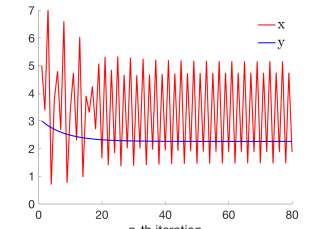
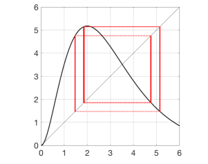
Figure 4: Bursting of period $4$ in the 2D Chialvo model (left) and the corresponding period $4$ orbit in the reduced model (right). See text for details.

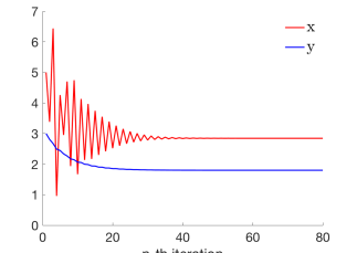
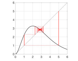
Figure 5: Resting of the voltage in the 2D Chialvo model (left) and the corresponding stable fixed point in the reduced model (right). See text for details.

Our bifurcation results (Thms 2.3, 2.5 and 2.7) confirm that a single neuron in the reduced Chialvo model is able to exhibit diverse activity regimes and periodic state transitions. Since quiescence plays the fundamental role in the analysis of neuronal activity, it seems to be crucial to describe the basic possible scenarios that fixed states of the model can undergo. Recall that the bifurcation parameters $r$ (Thms 2.3 and 2.5) and $k$ (Thm 2.7) coincide, respectively, with the recovery variable of the 2D Chialvo system and the additive voltage perturbation. Note that, in general, the flip bifurcation, which usually starts the period-doubling route to chaos (compare with Sec. 4), corresponds to transition from quiescence to regular tonic spiking, while the fold bifurcation corresponds to appearance of new resting states.

However, our main motivation behind studying the 1D Chialvo model is not to show that it well approximates the dynamics of the full 2D model but to point out that the 1D system itself represents very rich dynamics. Indeed, within some parameters range the behaviour of the 1D map might be even more complicated. For example, while experimenting numerically with the Chialvo model we have found that with the parameters set as $a=0.866$, $b=0.05$, $c=0.48$ and $k=0$ the trajectory starting from the initial conditions $(x_{\textrm{init}},y_{\textrm{init}})=(2.8,1.5)$ converges numerically to the period $4$ cycle $\{(x_{0},y_{0}),(x_{1},y_{1}),(x_{2},y_{2}),(x_{3},y_{3})\}$ with

$x_{0}$	$y_{0}$	$x_{1}$	$y_{1}$	$x_{2}$	$y_{2}$	$x_{3}$	$y_{3}$
$1.4646$	$2.2539$	$4.7230$	$2.3586$	$2.0970$	$2.2864$	$5.3144$	$2.3552$

On the other hand, the corresponding 1D model (with $k=0$ and $x_{\textrm{init}}=2.8$) showed period 4 periodic attractor for $r\in\{y_{0},y_{2}\}$, period 12 periodic attractor for $r=y_{3}$ and chaotic interval attractor for $r=y_{1}$, which agrees with our numerically obtained bifurcation diagram for the Chialvo map $f_{r}$ with $k=0$ (not shown here, but similar to that from Figure 7). In Figure 6 we present, starting from top left in clockwise direction, the time-series of $x$- and $y$-variables for the 2D model and the corresponding trajectories of the reduced model (with $x_{\textrm{init}}=2.8$ after removing a transient of 970 iterates) with $r=y_{0}$, $r=y_{1}$ and $r=y_{3}$, respectively. This behaviour exemplifies that sometimes the reduced model might, counter-intuitively, show more complicated dynamics than some of its 2D extensions. Therefore understanding of the 1D model bifurcation structure seems to be a relevant standalone topic.

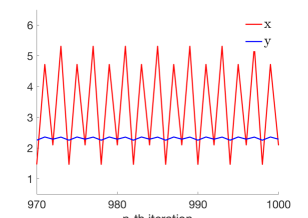
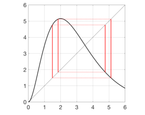
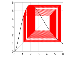
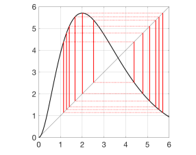
Figure 6: Regular period 4 bursting in the 2D model and the behaviour of the reduced model in the corresponding range of $r$ parameter values. See main text for details.

We close this section with Figure 7 which shows one-parameter bifurcation diagrams for the 1D Chialvo model, obtained in Python. One can observe that the $r$ dependence for the Chialvo family is similar to the parameter-dependence in the logistic family, whilst the $k$ dependence is similar to that in the Gauss family (with respect to the additive parameter).

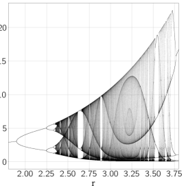
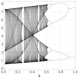
Figure 7: Bifurcation diagrams for the Chialvo family: versus $r$ with fixed $k=0.05$ (left) and versus $k$ with fixed $r=2.6$ (right).

3 Dynamical core of the Chialvo map

Recall that our definition of unimodality requires that either the left endpoint of the interval domain $I$ of the map $f$ is a fixed point with the right endpoint of the interval as its other preimage, or that $I=\left[f^{2}(c),f(c)\right]$, where $c$ is the critical point (maximum) of $f$. In this case we say that the interval $I$ is the dynamical core of $f$, i.e., the invariant interval where all nontrivial dynamics concentrates. An example of the dynamical core for some unimodal map is showed in Fig. 8.

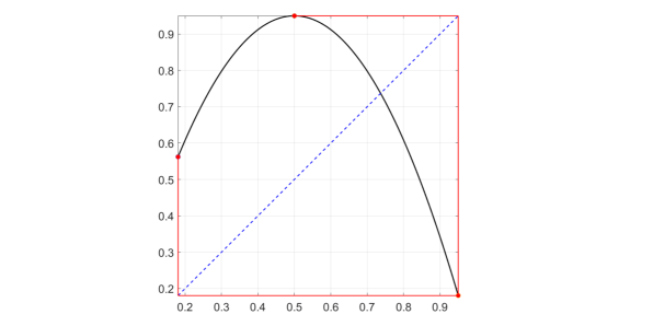
Figure 8: Interval $[f^{2}(c),f(c)]$ as a dynamical core ($c=1/2$ is a critical point)

Below we discuss the form of the dynamical core $I_{r,k}$ for $f_{r,k}(x)=x^{2}\exp(r-x)+k$ with respect to parameters $k$ and $r$ in order to justify that the map $f_{r,k}$ describing the 1D Chialvo model is S-unimodal on an appropriate subinterval of $[0,+\infty)$.

3.1 Case $k=0$

Let us firstly consider the case $k=0$ and the corresponding map $f_{r,0}(x)=x^{2}\exp{(r-x)}$. The map $f_{r,0}$ has exactly

• one fixed point $x_{0}=0$,

• two fixed points: $x_{0}=0$ and $x_{1}$ satisfying $0<x_{1}<2$,

• three fixed points: $x_{0}$, $x_{1}$ and $x_{2}$ satisfying $x_{0}=0$, $0<x_{1}<x_{2}$.

In the first two instances, the dynamics is trivial. Namely, every initial condition is attracted either by the superattracting fixed point $x_{0}$ or by the semistable fixed point $x_{1}$ (if exists). Configuration with three fixed points splits into two cases, the second with two subcases:

1. $x_{2}\leq 2$,

2. $x_{2}>2$: subcase 2.1. $x_{2}$ is stable, subcase 2.2. $x_{2}$ is unstable.

Of course, there is also a special case when $x_{2}=3$ undergoes flip bifurcation (when $2<x_{2}<3$, then $x_{2}$ is stable and if $x_{2}>3$ then it is unstable as follows from simple calculations in the part concerning flip bifurcation). The cases 1. and 2.1. are again trivial. Therefore for our further developments we shall be interested in case 2.2. Note that under this condition $x_{2}$ satisfies $x_{2}\exp(-x_{2})=\exp(-r)$ and for the derivative we have $|f^{\prime}_{r,0}(x_{2})|=|2-x_{2}|>1$. Therefore with the increase of $r$ the fixed point $x_{2}>3$ moves further to the right and remains unstable. Simultaneously the fixed point $x_{1}$ remains to the left of $c=2$ and is unstable. If, moreover, $x_{1}<f^{2}_{r,0}(2)$, then the interval $[f^{2}_{r,0}(2),f_{r,k}(2)]$ can be treated as the dynamical core of the map $f_{r,0}$, because every initial condition $x\in(x_{1},\infty)$ is after a few iterates mapped into $[f^{2}_{r,0}(2),f_{r,k}(2)]$. On the other hand, all the points in $(0,x_{1})$ are monotonically attracted to the resting state $x_{0}=0$. We are mainly interested in this case, i.e., when $x_{1}\notin[f^{2}_{r,0}(2),f_{r,0}(2)]$, which holds at least for some interval of $r$-values (see Lemma 3.1 and Remark 3.2).

3.2 Case $k>0$

Now let us consider the case $k>0$. Note that when $k\geq 2$, the dynamics of $f_{r,k}$ is actually trivial: indeed for $k\geq 2$ there is exactly one fixed point $x_{0}$ which is located on the right (decreasing) part of the graph (i.e. $x_{0}>k\geq 2$). As also $f_{r,k}^{2}(2)>k\geq 2$, the interval $[2,f_{r,k}(2)]$ is an invariant interval and every initial condition $x\in\mathbb{R}$ is after at most one iterate mapped into this interval. On the other hand, as $f_{r,k}$ is strictly decreasing on this interval, every initial condition $x\in\mathbb{R}\setminus\{x_{0}\}$ is actually attracted to $x_{0}$ (if $x_{0}$ is attracting) or to period two periodic orbit (if $x_{0}$ is not attracting). Obviously, in this case the dynamical core can be set as $[f^{2}(2),f(2)]$.

Therefore assume that $0<k<2$. Then (especially for small values of $r$) one possibility is that $f_{r,k}$ has only one fixed point $x_{0}$, which is located on the left branch: $x_{0}\leq 2$. Note that in this case $x_{0}$ is globally attracting and thus this is the trivial case. If $x_{0}$ is a unique fixed point but $x_{0}>2$, then, depending on $r$, the fixed point $x_{0}$ can be either stable or unstable, but, as $f^{2}_{r,k}(2)>k=f_{r,k}(0)$, we can set the interval $[f^{2}_{r,k}(2),f_{r,k}(2)]$ as the dynamical core, which contains exactly one fixed point $x_{0}>2$. Lemma 3.1 asserts that this always holds for $r$ large enough.

The situation when $f_{r,k}$ has exactly two fixed points is very rare (it holds e.g. when there is a fixed point $x_{0}>0$ and the other fixed point $x_{1}=x_{2}$ is just undergoing the fold bifurcation). Thus the effective complementary case for unique fixed point $x_{0}$ is the situation when there are exactly three fixed points $0<x_{0}<x_{1}<x_{2}$ and necessarily then $x_{1}\leq 2$. If also $x_{2}\leq 2$, then every initial condition (except $x_{1}$) is attracted either to $x_{0}$ or to $x_{2}$. It follows that for $0<k<2$ the non-trivial generic case with three fixed points is the situation when $0<x_{0}<x_{1}<2<x_{2}$ (with $x_{2}$ that can be stable or unstable). If $f_{r,k}^{2}(2)<x_{1}$, then as a dynamical core we set $[x_{0},y_{0}]$, where $y_{0}\in f_{r,k}^{-1}(x_{0})$ and $y_{0}\neq x_{0}$ (note that such a point $y_{0}$ exists since $f_{r,k}(x)\rightarrow k<x_{0}$ as $x\to\infty$). Then $f_{r,k}\colon[x_{0},y_{0}]\to[x_{0},y_{0}]$ matches the definition of the unimodal map. On the other hand, if $f_{r,k}^{2}(2)\geq x_{1}$, we can assume that the dynamical core is $[f_{r,k}^{2}(2),f_{r,k}(2)]$ (the map $f_{r,k}$ restricted to this interval is unimodal).

3.3 Auxiliary results on dynamical core

This subsection contains several results concerning the dynamical core of the 1D Chialvo map, which will be of our interest in the next section (for example in the proof of Theorem 4.9). The technical proofs of Lemmas 3.1 and 3.4 are postponed to Appendix A.

Lemma 3.1.

For any $0\leq k<2$ there exists $r^{*}=r^{*}(k)$ such that for all $r\geq r^{*}(k)$ we have

$$f_{r,k}^{2}(c)<c<f_{r,k}(c),$$ (5)

where $f_{r,k}(x)=x^{2}\exp(r-x)+k$ is the 1D Chialvo map and $c=2$ is its critical point. Moreover, for $k\neq 0$ the value of $r^{*}(k)$ can be chosen such that, in addition, for $r\geq r^{*}(k)$ the interval $[f_{r,k}^{2}(c),f_{r,k}(c)]$ contains exactly one fixed point $x_{f}$.

Remark 3.2.

For $k=0$, demanding that (5) is satisfied and simultaneously there are no fixed points in $[f_{r,0}^{2}(c),f_{r,0}(c)]$ to the left of $c$ requires some more specific range of $r$ values. Indeed, for $k=0$ the map can have three fixed points $x_{0}=0$, $0<x_{1}<2$ and $x_{2}>2$ with $x_{1}$ that actually can fall into the interval $[f_{r,0}^{2}(c),f_{r,0}(c)]$. We have verified numerically that for any $r\in[2.1,2.97]$ the inequality (5) is satisfied with $f^{2}_{r,0}(c)>x_{1}$. In turn, for $r=2$ we have $f_{r,0}^{2}(c)\approx 2.1654>c=2$ (violating (5)) and for $r=2.98$ $f_{r,0}^{2}(c)<x_{1}$ as $f_{r,0}^{2}(c)\approx 0.0526$ and $x_{1}\approx 0.0535$.

Remark 3.3.

Consequently, the interval $[f_{r,k}^{2}(c),f_{r,k}(c)]$ (in the proper parameter regime, i.e., $r\geq r^{*}(k)$ for $k\in(0,2)$ and $r\in[2.1,2.97]$ for $k=0$) can be treated as dynamical core of $f_{r,k}$, which contains exactly one fixed point, namely $x_{f}>2$.

The next lemma assures that with $r$ large enough the fixed point $x_{f}$ mentioned above is unstable.

Lemma 3.4.

For any $0\leq k<2$ there exists $r^{*}(k)$ such that for all $r\geq r^{*}(k)$ the map $f_{r,k}$ has an unstable fixed point $x_{f}>2$.

Corollary 3.5.

For every $k\in[0,2)$ there exists an interval $[r_{1},r_{2}]$ of positive $r$-values such that for any $r\in[r_{1},r_{2}]$ the map $f_{r,k}$ has an attracting fixed point $x_{f}>2$.

The above corollary can be easily justified taking into account the proof of Lemma 3.4 and the fact that for a S-unimodal map $f$ every fixed point $x_{f}$ with $|f^{\prime}(x_{f})|\leq 1$ is attracting.

4 Periodic versus chaotic behaviour

The 1D Chialvo map (2) except for regular behaviour due to the existence of stable fixed points or periodic orbits can also exhibit chaotic behaviour. There are many different notions of chaos (see ³⁶), with the most prominent one probably due to Devaney (³⁷). The common point of most of these definitions is some sort of sensitive dependence on initial conditions. In our approach we will consider both metric chaos associated with the existence of the absolutely continuous invariant probability measure (acip), which, as we recall below, for S-unimodal maps can be identified with some strong sensitive dependence on initial conditions, and topological chaos corresponding to the classical definitions of Li and Yorke, Block and Coppel, and Devaney.

4.1 Periodic attractors

Since the reduced Chialvo map is S-unimodal and its critical point is non-degenerate, the following two theorems are immediate consequences of Theorems 1.3 and 1.4.

Theorem 4.1.

The 1D Chialvo map (2) can have at most one periodic attractor and this attractor attracts the critical point $c=2$.

Let $\Gamma$ be a periodic orbit with period $n$ and let $\lambda(\Gamma)=(f^{n})^{\prime}(x)$ for $x\in\Gamma$. It is clear that $|\lambda(\Gamma)|\in[0,1)$ implies that $\Gamma$ is attracting. However, since $f$ is S-unimodal, by Theorem 1.3, also neutral periodic orbits (i.e. such that $|\lambda(\Gamma)|=1$) are attracting.

Theorem 4.2.

The 1D Chialvo map has a unique metric attractor $\mathcal{A}$ which is a limit set $\omega(x)$ for almost all initial conditions $x$. This attractor is either an attracting periodic orbit, a Cantor set of measure zero or a finite union of intervals with a dense orbit (so called interval attractor).

We say that two unimodal maps $f$ and $g$ are combinatorially equivalent if there exists an order-preserving bijection $h\colon\cup_{n\geq 0}f^{n}(c)\to\cup_{n\geq 0}\,g^{n}(c^{\prime})$ such that $h(f^{n}(c))=g^{n}(c^{\prime})$ for all $n\geq 0$, where $c$ and $c^{\prime}$ are critical points of $f$ and $g$. In the other words, $f$ and $g$ are combinatorially equivalent if the order of their forward critical orbit is the same.

Let us present the following general mathematical observation, which might be known to specialists in one-dimensional dynamics, but probably lacks clear references as follows, for example, from Remark 4.5 below.

Lemma 4.3.

Assume that $f$ and $g$ are S-unimodal maps. If $f$ has a period two attracting orbit and $g$ has a period three attracting orbit then $f$ and $g$ are not combinatorially equivalent.

Proof 4.4.

Let $\mathcal{A}$ denote a periodic attractor and $c$ a critical point. Since $\omega(c)=\mathcal{A}$, starting from some iteration the order of the critical point orbit is the same as the order on the periodic attractor. Obviously, the orders of a two and a three periodic orbit are different, which is our claim.

Remark 4.5.

In ³⁸ it is stated that a map with an attracting equilibrium and a map with a period two attracting orbit are not combinatorially equivalent, which in general is not true.

Let us also formulate a conjecture which generalizes Lemma 4.3, and which we believe is true.

Conjecture 1.

Let $f$ and $g$ be S-unimodal maps, $m>k$ and $m\neq 2k$. If $f$ has an attracting periodic orbit with a prime period $m$ and $g$ has an attracting periodic orbit with a prime period $k$, then $f$ and $g$ are not combinatorially equivalent.

The following useful result can be found in ³⁹ Th. C.

Theorem 4.6 (Kozlovski).

Let $\Lambda\subset\mathbb{R}^{k}$ be open and $\{f_{\lambda}\}_{\lambda\in\Lambda}$ be an analytic family of unimodal maps with a non-degenerate critical point and negative Schwarzian derivative. If there exist two maps in $\{f_{\lambda}\}$ that are not combinatorially equivalent, then there exists a dense subset $\Theta$ of $\Lambda$ such that $f_{\lambda}$ has a stable attracting periodic orbit for every $\lambda\in\Theta$.

The next result describes the subset in parameter space corresponding to periodic attractors.

Theorem 4.7.

The set of parameters for which the 1D Chialvo map $f_{r,k}$ has a stable attracting periodic orbit forms a dense subset of

1. the $r$ parameter space $\mathbb{R}$ when $k\in[0,2)$ is fixed,

2. the $(r,k)$ parameter space $\mathbb{R}\times[0,2)$.

Proof 4.8.

Let $k\in[0,2)$ be fixed. Clearly, for some $r$ the map $f_{r,k}$ has a period two attracting orbit and for some other $r$ it has a period three one. Consequently, Lemma 4.3 guarantees that the family $\{f_{r,k}\}$ contains two maps that are not combinatorially equivalent. Alternatively, to obtain two such maps we can use the kneading sequences from the proof of Corollary 4.13. Since all other assumptions of Theorem 4.6 are obviously satisfied, the assertion of the first statement of our theorem follows the Kozlovski Theorem. Finally, the second statement of our theorem follows from the first one.

4.2 Metric chaos

The following theorem guarantees that 1D Chialvo maps are strongly chaotic with positive frequency in parameter space. As we have mentioned above strong chaos here is associated with the existence of acip measure. Below we present the rigorous proof in the case $k=0$ and conclusions of numerical analysis for the case $k\in(0,0.58)$. Here and subsequently, $\delta_{x}$ denotes the Dirac measure at the point $x$ and $\operatorname{supp}(\mu)$ the support of a measure $\mu$. Moreover, recall that a map $f$ is called a Misiurewicz map if it has no periodic attractors and if critical orbits do not accumulate on critical points, i.e. when

$$C_{f}\cap\omega(C_{f})=\emptyset,$$

where $C_{f}$ denotes the set of critical points of $f$. For a parametrized family of maps $\{f_{r}\}$ the values of parameters for which $f_{r}$ are Misiurewicz maps are called Misiurewicz parameters. An example of such a parameter in the logistic family $Q(x)=\mu x(1-x)$ is $\mu=4$.

For fixed $k$, let $f_{r}(x):=x^{2}\exp{(r-x)}+k$ and let $I_{r}\subset[0,\infty)$ denote the dynamical core of $f_{r}$ (see Section 3 for details).

Theorem 4.9.

Let $k=0$ be fixed. There exists a positive Lebesgue measure set $\mathcal{R}$ such that for all $r\in\mathcal{R}$:

• the map $f_{r}:I_{r}\to I_{r}$ admits an absolutely continuous invariant probability measure $\mu_{r}$ such that

  $$\mu_{r}=\lim_{n\to\infty}\frac{1}{n}\sum_{i=0}^{n-1}\delta_{f_{r}^{i}(x)}\quad\text{for a.a.\ $x\in I_{r}$},$$ (6)

  i.e., $\mu_{r}$ describes the asymptotic distribution of almost all orbits under $f_{r}$,

• the unique metric attractor of the map $f_{r}$ is an interval attractor $\mathcal{A}_{r}$; moreover, $\mathcal{A}_{r}=\operatorname{supp}(\mu_{r})$ and $\mu_{r}$ is equivalent to the Lebesgue measure on $\mathcal{A}_{r}$.

In consequence, for each $r\in\mathcal{R}$ the Lyapunov exponent of $f_{r}$ is positive, i.e.,

$$\lim_{n\to\infty}\frac{1}{n}\log|\mathrm{D}f^{n}_{r}(x)|=\kappa_{r}>0\quad\text{for a.a.\ $x\in I_{r}$},$$ (7)

where $\mathrm{D}$ denotes the derivative with respect to $x$.

Proof 4.10.

The statements of the above theorem follow from some nowadays classical results on S-unimodal maps, for example, from Theorem 18 and Corollary 19 in ²⁹, provided that the below-listed conditions C1–C6 are satisfied for some interval of parameters $r$:

• $\{f_{r}\}$ is a one-parameter family of $C^{2}$ unimodal maps of an interval $I$ (in general the interval $I$ can vary with the change of the parameter $r$ , i.e. $I=I_{r}$),

• each $f_{r}$ has a nondegenerate critical point $c$,

• the map $(x,r)\mapsto(f_{r}(x),D_{x}f_{r}(x),D_{xx}f_{r}(x))$ is $C^{1}$,

• each $f_{r}$ has a repelling fixed point on the boundary of $I$,

• there is a parameter value $r^{*}$ such that the critical orbit is mapped onto an unstable periodic cycle $P^{*}$ in a finite number of steps (this implies that $f_{r^{*}}$ is a Misiurewicz map),

• the map moves with the parameter at $r^{*}$ in the following technical sense

  $$\frac{d}{dr}(x(r)-f_{r}(c))\big{|}_{r=r^{*}}\neq 0,$$

  where $x(r)$ is a point of $I$ and $P(r)$ is an unstable periodic orbit such that

  • $r\mapsto x(r)$ is differentiable,

  • $x(r^{*})=f_{r^{*}}(c)$,

  • $P(r)$ moves continuously with $r$,

  • $x(r)$ is mapped onto $P(r)$ in the same number of steps as $x(r^{*})$ and onto the corresponding point of $P(r)$

  (existence of such a point and orbit is guaranteed by the perturbation theory).

We are left with the task of checking all these conditions. We will see that in fact only C5–C6 might pose a problem.

Ad C1–C3. It is easy to see that in our situation the first three conditions do not require any justification.

Ad C4. The condition C4 can also be formally achieved by properly extending the map $f_{r}$ beyond its dynamical core $[f_{r}^{2}(c),f_{r}(c)]$ which does not effect its dynamics as all the points in $I$ will after a few iterates be mapped into the dynamical core. Recall that by Lemma 3.1 for each $k=0$ and $r=r(k)$ large enough we can set $[f_{r}^{2}(c),f_{r}(c)]$ as a dynamical core such that there are no fixed points in $[f_{r}^{2}(c),f_{r}(c)]$ except for $x_{f}$ located on the decreasing branch of $f$, i.e., $x_{f}>2$.

Ad C5. We will show that there exists a map $f_{r^{*}}$ such that the critical point $c$ is mapped in a few steps onto the unstable fixed point. Such a map is necessarily a Misiurewicz map. Let us only remind that Misiurewicz maps can be found in a number of ways and our idea of the proof is chosen for simplicity. We will call $r^{*}$ the Misiurewicz parameter.

Let us firstly justify that the fixed point $x_{f}>2$ is unstable for the $r$-parameter values used in further estimation of the Misiurewicz parameter. Let $x_{f}$ be a fixed point of $f(x)=x^{2}\exp{(r-x)}$. Then for $x_{f}\neq 0$ we have $x_{f}\exp(-x_{f})=\exp(-r)$. The right hand side of this equality decreases with $r$ and similarly the left one is a decreasing function of $x_{f}$ for $x_{f}>1$ (we are interested in $x_{f}>2$). Therefore the value of the fixed point $x_{f}>2$ also increases as $r$ increases, i.e. with the increase of $r$ the fixed point $x_{f}>2$ moves further to the right. Since $f^{\prime}(x_{f})=x_{f}\exp({r-x_{f}})(2-x_{f})=2-x_{f}$, $x_{f}$ is unstable whenever $x_{f}>3$. In our below estimation of the Misiurewicz parameter we consider $r\in(2.43,2.44)$. As for $r\geq 2.43$ we certainly have $x_{f}>3$, $x_{f}$ is unstable in this parameter range (taking into account the above arguments and our previous estimation of flip bifurcation $r$ value, $x_{f}$ remains unstable fixed point for all $r>r_{0}\approx 1.901$).

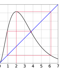
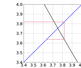
Figure 9: Lower estimation of the Misiurewicz parameter (case $k=0$): $d(r)>0$ for $r=2.43$. Left: iterations of the critical point. Right: close-up of cobweb around the fixed point.

We show the existence of the Misiurewicz parameter in the interval $r\in(2.43,2.44)$. Namely, we prove that for the parameter value $r^{*}\approx 2.436$ the critical point $c=2$ is mapped onto the unstable fixed point after exactly three iterations. We make use of the cobweb diagram, instead of using numerical approximations methods. Let $d(r)$ be the distance between the third iteration of the critical point $x_{c}=2$ and the corresponding fixed point $x_{f}(r)$, i.e., $d(r)=f^{3}(2,r)-x_{f}(r)$. Although we do not have an explicit expression for the fixed point, $d(r)$ represents a smooth function in $r$. Since $d(r)$ changes sign in the interval $2.43<r<2.44$, that is illustrated in Figures 9–10, by the Intermediate Value Theorem there exists $r^{*}\in(2.43,2.44)$ such that $d(r^{*})=0$, and therefore the critical point is mapped onto the fixed point in three iterations. Note that in this way we have obtained actually a rigorous proof of the existence of a Misiurewicz map and the numerics were only used for estimation of the Misiurewicz parameter.

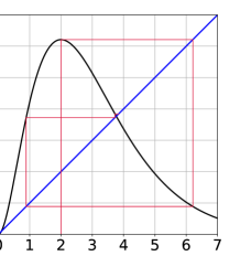
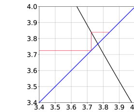
Figure 10: Upper estimation of the Misiurewicz parameter (case $k=0$): $d(r)<0$ for $r=2.44$. Left: iterations of the critical point. Right: close-up of cobweb around the fixed point.

Ad C6. We will verify the condition $C6$ numerically as in ²⁹. Let us define $f(x,r)=f_{r}(x)$, and $f^{n}(x,r)=f(f^{n-1}(x,r),r)=f^{n}_{r}(x)$ for $n>1$. For $r$ close to $r^{*}$ we may define $\zeta(r)$ by the formulas

$$\zeta(r^{*})=f_{r^{*}}(c)\quad\text{and}\quad f^{2}(\zeta(r),r)=z(r),$$

where $c$ is the critical point and $z(r)$ is an unstable fixed point of $f_{r}$ (see Lemma 3.4). This means that $\zeta(r)$ is a point close to $f_{r}(c)$ with the same type of forward orbit as $f_{r^{*}}(c)$. We abbreviate $f(\zeta(r),r)$ to $\zeta_{1}(r)$. The condition C6 now reads

$$\frac{d}{dr}(\zeta(r)-f(c,r))\big{|}_{r=r^{*}}\neq 0.$$

By the definition of $\zeta$, we have:

$$\begin{split}\frac{d\zeta}{dr}&=\Big{(}\frac{\partial f}{\partial x}(\zeta,r)\Big{)}^{-1}\bigg{\{}\Big{(}\frac{\partial f}{\partial x}(\zeta_{1},r)\Big{)}^{-1}\Big{(}\frac{dz}{dr}-\frac{\partial f}{\partial r}(\zeta_{1},r)\Big{)}-\frac{\partial f}{\partial r}(\zeta,r)\bigg{\}}\\ &=\frac{dz}{dr}\cdot\frac{\exp(\zeta+\zeta_{1}-2r^{*})}{\zeta\zeta_{1}(2-\zeta)(2-\zeta_{1})}-\frac{\zeta_{1}\exp(\zeta-r^{*})}{\zeta(2-\zeta)(2-\zeta_{1})}-\frac{\zeta}{2-\zeta}.\end{split}$$ (8)

Observe that all the partial derivatives in (8) can be computed explicitly. To find the value of $\frac{dz}{dr}$ we differentiate the implicit formula for fixed points $z^{2}\exp(r-z)=z$, which gives $\frac{dz}{dr}=\frac{z}{z-1}$. In consequence, to check the condition C6, we need only the previous estimation of the Misiurewicz parameter ($r^{*}\approx 2.436$) and the similar estimation of the corresponding fixed point ($z(r^{*})\approx 3.761$). The final calculations (done in MATLAB) are presented in the first column of Table 1. As we see $\frac{d}{dr}(\zeta(r)-f(c,r))\big{|}_{r=r^{*}}\approx-3.851$, so it is nonzero, which shows that the condition C6 is satisfied and completes the proof.

Table 1: Data for estimation of $\Gamma=\frac{d}{dr}(\zeta(r)-f(c,r))\big{|}_{r=r^{*}}$ for some $k$ in $[0,0.58]$.

$\begin{array}[]{lrrrrrrr}\hline\cr\hline\cr\text{term}&k=0&k=0.01&k=0.1&k=0.3&k=0.5&k=0.55&k=0.58\\ \hline\cr r^{*}&2.436&2.439&2.461&2.535&2.681&2.759&2.851\\ \hline\cr z(r^{*})&3.761&3.768&3.830&3.999&4.254&4.367&4.491\\ \hline\cr\zeta=\zeta(r^{*})&6.186&6.215&6.443&7.130&8.403&9.095&9.948\\ \hline\cr\zeta_{1}=\zeta_{1}(r^{*})&0.900&0.895&0.874&0.814&0.731&0.697&0.662\\ \hline\cr\frac{d\zeta}{dr}(r^{*})&2.335&2.335&2.383&2.594&3.491&4.433&6.426\\ \hline\cr\frac{\partial f}{\partial r}(c,r^{*})&6.186&6.205&6.343&6.830&7.903&8.545&9.368\\ \hline\cr\Gamma=\frac{d\zeta}{dr}(r^{*})-\frac{\partial f}{\partial r}(c,r^{*})&-3.851&-3.870&-3.960&-4.236&-4.412&-4.112&-2.942\\ \hline\cr\hline\cr\end{array}$

Remark 4.11.

Unfortunately, when $k>0$ we are not able to prove rigorously that the conditions C5 and C6 are satisfied for all $k$ in this range. However, we can provide numerical justification of both the existence of the Misiurewicz parameter $r^{*}$ (C5) and the nonzero value of the term $\Gamma=\frac{d}{dr}(\zeta(r)-f(c,r))\big{|}_{r=r^{*}}$ (C6) for some values of the parameter $k$ between $0$ and $0.58$. Recall that, by Lemma 3.4, for any $0<k<2$ there exists $\widehat{r}=\widehat{r}(k)$ such that for all $r\geq\widehat{r}$ the map $f_{r}$ has an unstable fixed point $x_{f}>2$. It occurs that for $k\in(0,0.58]$ one can proceed in much the same way as in the case $k=0$ to show that there exists $r^{*}$ such that the map $f_{r^{*}}$ is a Misiurewicz map. We simply search for $r^{*}$ such that the third iteration of the critical point is mapped onto the unstable fixed point (this method does not work for $k>0.58$). The calculation of the term $\Gamma$ are also similar as in the case $k=0$. The formula (8) still holds, but $\frac{dz}{dr}=\frac{z^{2}}{\exp(z-r)+z^{2}-2z}$ for $k>0$. The results of our numerical analysis are summarized in Table 1. Note that only the last row of Table 1 does not display monotonic behaviour. Finally, in Figure 11 we present plots of the Misiurewicz parameter $r^{*}$ and the term $\Gamma$ from the condition C6 as functions of the parameter $k\in[0,0.58]$ (in both cases the step size is $0.001$). Observe the rapid growth of the value of $\Gamma$ near $k=0.58$.

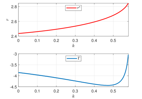
Figure 11: The Misiurewicz parameter $r^{*}$ (upper plot) and $\Gamma=\frac{d}{dr}(\zeta(r)-f(c,r))\big{|}_{r=r^{*}}$ (lower plot) as functions of the parameter $k\in[0,0.58]$ (step size $0.001$).

We finish this subsection with a result showing that in the Chialvo model two cases (periodic attractors and acips) occupy a set of full measure in parameter space. Namely, the following classical theorem from ⁴⁰ Th. B can be applied in the analysis of the reduced Chialvo map. The original result is more general, as it considers the class of quasiquadratic maps, which contains S-unimodal maps with a non-degenerate critical point. Recall that a one-parameter family of S-unimodal maps is called trivial if all maps have the same kneading sequence and the multipliers of any non-repelling orbits are the same for all maps.

Theorem 4.12 (Avila, Lyubich, de Melo).

Let $\Lambda\subset\mathbb{R}$ be open and let $\{f_{\lambda}\}_{\lambda\in\Lambda}$ be a non-trivial real-analytic family of S-unimodal maps with a non-degenerate critical point. Then for Lebesgue-almost all parameter values $\lambda\in\Lambda$ the map $f_{\lambda}$ has either a periodic attractor (such a map is called regular) or an interval attractor supporting an acip (such a one is called stochastic).

Proposition 4.13.

If $k\in[0,2)$ is fixed then for Lebesgue-almost all parameters $r$ the 1D Chialvo map $f_{r}$ has either a periodic attractor or an interval attractor supporting an acip.

Proof 4.14.

It suffices to show that the 1D Chialvo family with respect to $r$ is non-trivial. However, when $k\in[0,2)$ our family contains two maps with the kneading sequences of the form $(CC\dotsc)$ (the critical point is fixed) and $(C1\dotsc)$ (the critical point is on the left from the fixed point), which is our claim.

4.3 Topological chaos

Let us start this subsection with three classical definitions of topological chaos for discrete dynamical systems given by Li and Yorke (⁴¹), Block and Coppel (⁴²) and Devaney (³⁷). The relations among these three definitions of chaos for continuous maps are comprehensively explained in ³⁶. Recall that $\Sigma$ denotes the sequence space on the two symbols $\{\alpha=(a_{0}a_{1}a_{2}\dotsc)\mid a_{i}=0\text{ or }a_{i}=1\}$ with the metric $d(\alpha,\beta)=\sum_{i=0}^{\infty}{\left\lvert a_{i}-b_{i}\right\rvert}/{2^{i}}$. The shift map $\sigma\colon\Sigma\to\Sigma$ is given by $(a_{0}a_{1}a_{2}\dotsc)\to(a_{1}a_{2}a_{3}\dotsc)$. From now on assume that $X$ is a compact metric space and $f\colon X\to X$ is continuous.

Definition 4.15 (L/Y-chaos).

A map $f$ is called chaotic in the sense of Li and Yorke (L/Y-chaotic for short) if there exists an uncountable subset $S$ (called scrambled set) of $X$ with the following properties:

1. $\limsup\limits_{n\rightarrow\infty}{d(f^{n}(x),f^{n}(y))}>0$ for all $x,y\in S$, $x\neq y$,

2. $\liminf\limits_{n\rightarrow\infty}{d(f^{n}(x),f^{n}(y))}=0$ for all $x,y\in S$, $x\neq y$,

3. $\limsup\limits_{n\rightarrow\infty}{d(f^{n}(x),f^{n}(p))}>0$ for all $x\in S$, $p\in X$, $p$ periodic.

Definition 4.16 (B/C-chaos).

A map $f$ is called chaotic in the sense of Block and Coppel (B/C-chaotic for short) if there exists $m\in\mathbb{N}$ and a compact $f^{m}$-invariant subset $Y$ of $X$ such that $f^{m}|_{Y}$ is semi-conjugate to the shift on $\Sigma$, i.e., if there exists a continuous surjection $h\colon Y\to\Sigma$ satisfying $h\circ f^{m}=\sigma\circ h$ on $Y$.

Definition 4.17 (D-chaos).

A map $f$ is called chaotic in the sense of Devaney (D-chaotic for short) if there exists a compact invariant subset $Y$ (called a D-chaotic set) of $X$ with the following properties:

1. $f|_{Y}$ is topologically transitive,

2. the set of periodic points $\textrm{Per}(f|_{Y})$ is dense in $Y$, i.e., $\overline{\textrm{Per}(f|_{Y})}=Y$,

3. $f|_{Y}$ has sensitive dependence on initial conditions.

The following result provides the sufficient condition for the existence of topological chaos in the 1D Chialvo model in all the above senses.

Theorem 4.18.

If the 1D Chialvo map $f$ satisfies the condition

$$f^{2}(c)<f^{3}(c)<c<f(c)\quad\text{($c=2$ is the critical point)},$$ (9)

then it is chaotic in the sense of Li and Yorke, Block and Coppel, and Devaney.

Proof 4.19.

Let $x_{0}=c$ and $x_{i}=f(x_{i-1})$ for $i=1,2,3$. By the Intermediate Value Theorem, the map $f\colon[x_{0},x_{1}]\to[x_{2},x_{1}]$ has a unique fixed point $z\in(x_{0},x_{1})$. Observe that

$$f\big{(}[x_{2},x_{0}]\big{)}=[x_{3},x_{1}]\supset[z,x_{1}]\quad\text{and}\quad f\big{(}[x_{0},z]\big{)}=[z,x_{1}]$$

and, in consequence,

$$[x_{2},z]=[x_{2},x_{0}]\cup[x_{0},z]\subset f^{2}\big{(}[x_{2},x_{0}]\big{)}\cap f^{2}\big{(}[x_{0},z]\big{)}.$$

Hence $f^{2}$ is turbulent, i.e., there are nonempty closed subintervals $J$, $K$ of $[x_{2},x_{1}]$ with disjoint interiors such that $J\cup K\subset f^{2}(J)\cap f^{2}(K)$. By ³⁶ Prop. 3.3, the map $f\colon[x_{2},x_{1}]\to[x_{2},x_{1}]$ is B/C-chaotic. Moreover, by ³⁶ Th. 4.1, this is equivalent to being D-chaotic and, by ³⁶ Th. 4.2, this implies being L/Y-chaotic.

Remark 4.20.

It is worth pointing out that according to the above definitions of chaos the map is chaotic if it displays chaotic behaviour on a nonempty compact invariant subset of the dynamical core (not necessarily on the whole domain interval) and this set can be small both in the sense of measure and category. Notice also that the above proof works for an arbitrary unimodal map, whose critical point satisfies (9).

It occurs that the sufficient condition from Theorem 4.18 is actually satisfied for some range of parameters in the Chialvo model.

Proposition 4.21.

For $k=0$ and $2.6\leq r\leq 2.9$ the 1D Chialvo map $f_{r}$ satisfies (9) and, in consequence, is chaotic in the sense of Li and Yorke, Block and Coppel, and Devaney.

The technical proof of Proposition 4.21 is postponed to Appendix B.

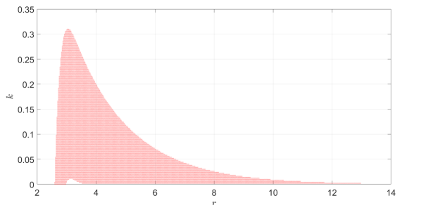
Figure 12: Topological chaos values (red dots) for the 1D Chialvo model in $(r,k)$ parameter plane.

Remark 4.22.

When $k>0$, by means of numerical simulations, we are able to observe a dependence between values of $r$ and $k$ for which the condition (9) from Theorem 4.18 is satisfied. However, it is difficult to obtain an interval for $r$ where all the inequalities are satisfied independently of the values of $k$. Figure 12 below depicts the result of a numerical simulation in MATLAB. We plot values of $r$ and $k$ for which the condition (9) is satisfied. The intervals of study for both parameters are: $2\leq r\leq 14$ with step size $0.025$ and $0\leq k\leq 0.35$ with step size $0.002$. The short of the program and the table with computed parameter values can be found in an open repository ⁴³.

4.4 Conclusions for the neuron activity analysis

It should be emphasized that the standalone 1D model (2) is able to reproduce a wide range of interesting neuronal behaviours (similarly to its 2D counterpart). In Figure 13 we show two examples of voltage trajectories. The trajectory with initial condition $x_{\textrm{init}}=2.2$ and parameter values $k=0.1$ and $r=2.45$ displays ‘chaotic’ spiking with subthreshold oscillations (depicted on the left), which can be also classified as (non-regular) MM(B)Os (mixed-mode (bursting) oscillations), i.e., spikes (or bursts) interspersed with small (‘subthreshold’) oscillations. Note that Theorem 4.9 guarantees that for $k=0$ the set of parameters $r$ for which the model exhibits ‘strongly chaotic’ behaviour (chaotic spiking/ bursting, irregular MMOs, etc.) is ‘observable’ (has a positive Lebesgue measure). However, the estimation of its actual size is a completely different and much harder task (see for instance ⁴⁴). Moreover, for $k=0$ ‘weak chaotic’ behaviour of the model is even more clearly ‘visible’ as, according to Proposition 4.21, it occurs for the set of parameters $r$ containing a ‘quite big’ interval.

On the other hand, for the same value of $r$ and $k$ increased to $k=0.2$ the neuron with initial voltage value $x_{\textrm{init}}=2.25$ exhibits, after initial adaptation, regular MMOs (depicted on the right). In this case, both spikes and subthreshold (non-spikes, i.e. low amplitude) oscillations occur periodically. Observe that, according to Theorem 4.7, periodicity and asymptotic periodicity (periodic spiking/bursting, phasic spiking/bursting, regular MMOs, etc.) are the most ‘common’ types of behaviour of the model under consideration.

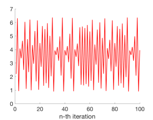
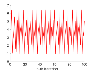
Figure 13: Chaotic spiking with subthreshold oscillations (left) and regular mixed-mode oscillations after initial adaptation (right) in 1D Chialvo model (for parameter values see main text).

It is worth notifying that MM(B)Os can play an important role in neuron’s information processing but for non-discrete models can occur only in higher dimensions (continuous models require at least three dimensions and for hybrid models, with continuous subthreshold dynamics, starting from two dimensions, see ⁷). Actually, during our numerical experiments with the 1D Chialvo model we have also encountered, e.g. regular tonic spiking and phasic spiking.

Moreover, observe that, due to Theorem 4.2, if we restrict ourselves to the dynamical core, then the reduced Chialvo model cannot directly exhibit bistable behaviour (coexistence of periodic and chaotic attractors) for fixed values of parameters $r$ and $k$, because the 1D Chialvo map admits a unique metric attractor, which in general is periodic, solenoidal or interval, but with full probability periodic or interval (see Prop 4.13). However, chaotic behaviour in the dynamical core can, of course, coexist with an attracting fixed point outside the dynamical core. Moreover, the substitute of bistability effect, i.e., interweaving of periodic and chaotic attractors in the 1D model can be also observed while varying the parameter $r$ corresponding to the second (recovery) variable of the 2D model. This is formally assured by Theorems 4.7 and 4.9.

Various oscillations modes in the reduced Chialvo model, as we have seen, are closely related to the existence of periodic attractors. Restricting the domain of the initial conditions to the dynamical core, we know that there is at most one attracting periodic orbit since the map is $S$-unimodal. Hence if the $1D$ model exhibits periodic oscillations, then this (asymptotically) periodic spike pattern is unique among observed oscillations modes (for fixed parameters $r$ and $k$). The arrangement of smaller and larger oscillations (spikes) and their amplitudes depend on the itinerary of this attracting periodic orbit. In particular, period-two attracting orbit (with points on different sides of the critical point $c$) corresponds to tonic regular spiking (when each spike has the same amplitude and length of each interspike-interval is the same). However, for many parameter values the system exhibits also chaotic-like (not regular) oscillations since there are ranges of parameters when the map is chaotic. Therefore determining values of parameters corresponding to various oscillations modes firstly demands providing exact bifurcation diagram of the map $f_{r,k}$ in the $(r,k)$-plane. This, however, would be a very challenging task since even with one parameter fixed the system undergoes cascades of rapid bifurcations. This is exemplified in Figure 7. In fact, left panel of this figure allows to conclude, approximately, values of $r$ (for $k=0.05$ fixed) corresponding to resting and periodic oscillations with period $2$, $4$, $8$ (and perhaps more) as well as ranges of chaotic (or very large period) oscillations. The second panel of this figure provides analogous information for varying $k$ and $r=2.6$ fixed. Note, however, that in all the cases, small change of the parameter might cause onset of chaos or quite sudden disappearance of chaotic behaviour. Approximate regions in $(r,k)$-parameter space when chaotic oscillations might occur might be deduced from the red area depicted in Figure 12.

4.5 Remarks on the 2D Chialvo model

Although, this work is concerned with 1D reduction of the Chialvo model, for completeness let us discuss some properties of the system (1a)-(1b) which might indicate interesting pathways for further studies.

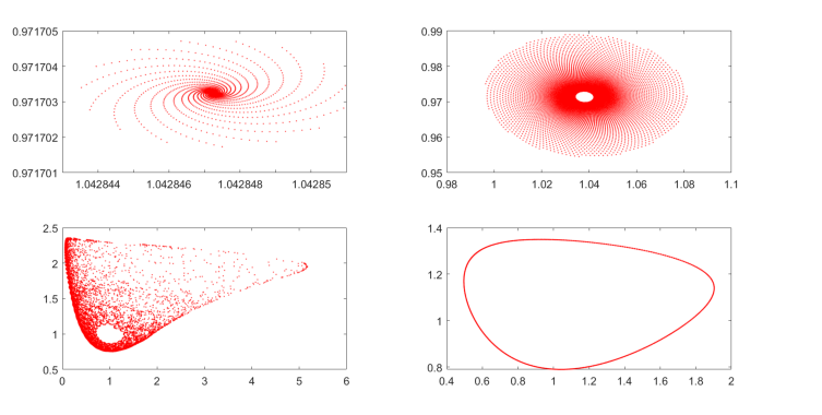
Figure 14: Numerical attractors in the 2D Chialvo model for the fixed values of $a=0.89$, $c=0.28$, $k=0.03$ and four different values of $b:0.166,\,0.1668,\,0.169,\,0.1738$ (clockwise from upper left corner)

The work of Chialvo ⁹ discusses the case of $k=0$ and $k$ of small positive value keeping fixed values of parameters $a$ and $c$ and only varying $b$ when needed. The parameter $k$ is treated as the bifurcation parameter. As mentioned in Introduction, for $k=0$, the point $(x_{\textrm{f}\,0},y_{\textrm{f}\,0}):=(0,c/(1-a))$ is always a stable fixed point of the system. For $k\neq 0$ the system (1a)–(1b) can have up to three fixed points.

Chialvo ⁹ treats only the case when the phase portrait has exactly one equilibrium point and the values of parameters $a$ and $c$ are fixed as $a=0.89$ and $c=0.28$. Nevertheless, even in this prescribed regime of parameters the system features rich behaviour which is directly matched with activity properties of neurons. With this choice of parameters $a$ and $c$, small values of $k$ (e.g. $k=0.02$) and $b=0.6$ the unique fixed point is globally attracting and the system is quiescent-excitable since it can generate an action potential when properly stimulated but is not able to maintain oscillatory spiking. Increasing $k$ (while keeping other parameters fixed) causes fixed point loses stability and oscillatory behaviour appears (bifurcation from quiescent-excitable to oscillatory solution). Obviously, the $2D$ model is also able to exhibit chaotic-like behavior which Chialvo ⁹ observed e.g. for $k=0.03$ and $b=0.18$ (and $a=0.89$, $c=0.28$ as stated). In this case the model displays chaotic mixed-mode oscillations (bursting oscillations with large spikes often followed by oscillations of smaller amplitude, see Figure 10 therein).

However, as we already mentioned, the system (1a)–(1b) can have up to three fixed points. Their existence, stability and bifurcations were studied in ¹⁸. In particular, the authors provided explicit conditions when the $2D$ Chialvo system has a given number of fixed points and theorems establishing the existence of fold, flip bifurcation and Hopf bifurcations. They have also proved the existence of chaos in the sense of Marotto. These analytical studies are then complemented by numerical simulations which in addition reveal e.g. various period-doubling bifurcations and different routes to chaos, sudden disappearance of chaos and strange chaotic and nonchaotic attractors. In the analytical part they treat $k$ as a bifurcation parameter but interestingly allow also negative values of $k$. On the other hand, in the numerical part they consider also non-autonomous Chialvo model where the external stimulus is periodic and the amplitude or frequency of this input can be a bifurcation parameter.

In a recent short communication paper ¹⁹, the authors, contrary to other studies, consider $(a,b)$-parameter space where $c$ and $k$ are fixed. These studies are numerical but illustrate the existence of interesting structures. In particular, they suggest Neimark–Sacker bifurcation of the fixed point and mode locking behaviour. The location of parameter regions corresponding Neimark–Sacker bifurcation and the birth of Arnold tongues are determined analytically. They have also numerically identified comb-shaped periodic regions (corresponding to period-incrementing bifurcations) and shrimp-shaped structures immersed in large chaotic regions.

Finally, the recent preprint ⁴⁵ undertakes the analysis of the 2D Chialvo model combining rigorous numerical methods and a topological approach based on the Conley index and Morse decompositions which allows to split considered range of parameters into classes of equivalent dynamics. However, again due to the computational complexity of this $4$-parameters dependant system, the authors fix $a=0.89$ and $c=0.28$ (similarly as in Chialvo paper ⁹) and explore some rectangular area of $b>0$ and $k>0$. Their study is enriched with the analysis of chain-recurrence properties of sets and additionally incorporates machine learning for identifying parameter ranges that yield chaotic behaviour.

Figure 15: Time series of the voltage $x$ for the numerical attractors of the 2D Chialvo model from Fig. 14

Although the current work is concerned with 1D Chialvo model, we have performed numerous simulations of the 2D model. We have decided to include only some of them in this work. This is due to the fact that the model is extremely sensitive to any, sometimes even arbitrary small, changes of parameters that can lead to very different behaviours. Indeed, in Fig. 14 we present numerically obtained representative phase portraits for $a=0.89$, $c=0.28$, $k=0.03$ and four different values of $b$ ($0.166$, $0.1668$, $0.169$, $0.1738$, respectively). Each picture presents a typical trajectory of the system after removing the transient part. Thus these pictures show various types of possible attractors for the 2D model. We see that increasing $b$ in such a small range of values, while keeping all the other parameters fixed, causes shifting the dynamics from the one corresponding to the attracting focus, through periodic limit cycle, to chaotic oscillations where both the interspike intervals and the number of small oscillations between consecutive spikes vary. Looking at Fig. 14 we can suspect that the system firstly undergoes bifurcation when the globally attracting fixed point loses its stability and the stable limit cycle appears and soon after that another bifurcation when asymptotically periodic dynamics is replaced by chaotic one. Corresponding voltage traces are presented in Fig. 15.

Our brief investigation of the 2D model and the mentioned works ^{9, 18, 19, 45} provide insightful and valuable observations. However detailed dynamical picture of the 2D Chialvo model is still very incomplete. This is mainly due to the fact that discrete systems, even in low-dimenions such as the Chialvo model, yield more challenges in their analytical (and numerical) analysis. Indeed, in planar continuous systems (i.e. systems defined by ODEs) one has e.g. Poincaré-Bendixson Theorem which allows to draw conclusions on the asymptotic behaviour of trajectories (by describing possible types of invariant limit sets). In particular, in 2D continuous systems chaotic dynamics is excluded, whereas in discrete settings one can observe chaos even in 1 dimension (i.e on the interval or on the circle). The second reason is the nature of the Chialvo model itself, by which we mean, and as we demonstrated, that the model is very sensitive to even very small change of parameters as it happens that in the very small region of parameter space it might undergo not one, but a couple of bifurcations. This in turn makes validation of the numerical analysis of the model challenging and emphasis the need for rigorous analytical studies which, however, due to the above mentioned reasons are especially hard. Therefore our aim was to show that even the reduced Chialvo model can be interesting for the mathematical analysis and not necessarily less plausible than its full version.

Discussion

We have performed detailed analysis of the reduced Chialvo model (2) which describes the evolution of the membrane voltage when recovery variable is frozen, i.e., becomes a parameter. Let us briefly summarize these results here.

Firstly, we established that the model (2) can be seen as iterations of the S-unimodal map $f_{r}$, which opened the way to prove its various properties with the use of the powerful theory of S-unimodal maps (and, more general, maps with negative Schwarzian derivative). In Theorems 2.3, 2.5 and 2.7 we rigorously showed that the model undergoes flip and fold bifurcations of fixed points when $r$ is a bifurcation parameter and a fold bifurcation with respect to $k$ parameter, providing formulas for the bifurcation parameter values and fixed points involved. In particular, due to the fact that Schwarzian derivative is negative, all the flip bifurcations are supercritical.

Next, discussing different configurations of the map with respect to the number and location of its fixed points and precising what should be treated as dynamical core of the map we justified that the map can be in fact viewed as an S-unimodal map. Moreover, Lemmas 3.1 and 3.4 asserts that for wide range of $(r,k)$ parameter space in the dynamical core of the map there is only one fixed point which is unstable. This instability of the fixed point played role in justifying the existence of Misiurewicz maps in the family $\{f_{r}\}$ (with $k$ fixed) and showing that for positive Lebesgue measure set of parameters these maps admit an absolutely continuous invariant probability measure (acip) with positive Lyapunov exponent for almost all initial conditions (see Theorem 4.9 and following discussion). In all these cases, the map has an interval attractor which is the support of the acip. This situation is often referred to as metric chaos. The effective complementary case (see Proposition 4.13) is when the map $f_{r}$ has a periodic attractor which is then necessarily unique (Theorem 4.1). This fact has some implications for the numerics, i.e. in the regime of the existence of stable periodic orbit, its uniqueness and the fact that it attracts almost all initial conditions, guarantees that by randomly choosing initial point $x_{0}$ and iterating it under the one-dimensional Chialvo map we can reconstruct this periodic attractor. Abundance of this periodic case is captured in Theorem 4.7. On the other hand, Theorem 4.18 gives the combinatorial condition for the map to be chaotic in the sense of Li and Yorke, Block and Coppel, and Devaney. Proposition 4.21 and further numerical analyses estimate the subset of $(r,k)$ parameter space where this topological chaos occurs.

As argued in some references and mentioned in Introduction, the equation (2) sometimes qualitatively approximates the dynamics of voltage-variable in the full model (1a)–(1b), especially when it can be viewed as a slow-fast system with the slow variable $y$, virtually frozen or acting as a slowly varying bifurcation parameter of the fast subsystem. However, the form of the full model (1a)–(1b) does not allow for an easy and explicit separation of time-scales unless the $a$, $b$ and $c$ parameter values are specifically chosen. Therefore, although the slow-fast nature of the system for some parameters’ values is reflected in numerical simulations (see e.g. ⁹), rigorous application of singular perturbation theory for this model and, perhaps, revealing implications of our finding for the full model, can be a separate task for future research. Another approach can rely on using the theory of discrete-time nonautonomous dynamical systems (see e.g. ⁴⁶) for inferring the $x$-dynamics in the full system. However, as revealed e.g. by the numerical experiments related to Figure 6, sometimes the behaviour of the reduced model might be more complicated than that of the 2D model within the corresponding area of the phase plane. This of course depends on the parameter choice in the 2D model but also, together with the variety of activity modes which the model is able to display (as illustrated e.g. in Figures 4, 5 and 13), serves in favour of the argument that 1D model might be treated as the independent model and that, perhaps, it would be worth considering other variants of the 2D model with the same equation for the membrane voltage but different types of the recovery dynamics. In any case, the starting point for creating such new variants of the Chialvo model would be to fully understand the evolution of the membrane voltage given by (2), which this paper aims at.

Moreover, as pointed also in ¹⁷, the Chialvo model does not fit exactly into the scheme of slow-fast neuron models with $x$ being the fast variable and $y$ the slow variable (in fact, $y$ might even represent the fast, not the slow, variable), because the impact of $y$ onto the voltage evolution equation is not additive but multiplicative and thus changing $y$ does not simply shifts the map $f$ upward or downward. Therefore understanding the bifurcation structure of the map $f_{r,k}$, especially with respect to $r$ parameter, is very important and was another motivation behind this work.

On the other hand, providing complete description of the dynamics of the full model (1a)–(1b) (corresponding to different parameters configuration in the $(a,b,c,d,k)$ space, or its $(b,k)$ subspace), seems challenging. The works ⁹ and ¹⁸ gave some initial results in this direction but this extensive task demands other supporting methods, for instance, topological and computational dynamics tools (identifying invariant sets and their Conley indices) and might be a base for future works. From that point of view, presented here, rather complete, dynamical description of the somehow independent 1D model seems to be very natural and useful.

Appendix A Proofs of results on the dynamical core

Proof A.1 (Proof of Lemma 3.1).

The second inequality $c<f_{r,k}(c)$ is straightforward and moreover if we demand only this inequality it is enough to set $r^{*}(k)=r^{*}(0)$ for any $k\geq 0$. In order to prove the first inequality we compute $f_{r,k}^{2}(c)=(4\exp(r-2)+k)^{2}\exp\{r-4\exp(r-2)-k\}+k$, which can be further expanded as

$$f_{r,k}^{2}(c)=\left\{16\exp(3r-4-k)+8k\exp(2r-2-k)+k^{2}\exp(r-k)\right\}\exp\{-4\exp(r-2)\}+k.$$

Since for large $r$ (with fixed $k\in[0,2)$)

$$\exp\{-4\exp(r-2)\}\leq\min{\{\exp(-4r+4+k),\exp(-3r+2+k),\exp(-2r+k)\}},$$

we have

$$f_{r,k}^{2}(c)\leq\left\{16+8k+k^{2}\right\}\exp(-r)+k<2$$

for sufficiently large $r$, which proves (5).

Note that the second statement about the unique fixed point in the interval $[f_{r,k}^{2}(c),f_{r,k}(c)]$ means that there are no fixed points $x_{f}$ on the increasing part of the graph of $f_{r,k}$ with $x_{f}\geq f_{r,k}^{2}(c)$ (as necessarily the interval $[f_{r,k}^{2}(c),f_{r,k}(c)]$ contains the fixed point $x_{f}>2$). Thus let $0<k<2$. In this case for $r$ large enough and $k\leq x\leq 2$ the following sequence of inequalities holds:

$$\exp(r-x)\geq\exp(r-2)>\frac{1}{k}-\frac{k}{4}\geq\frac{1}{x}-\frac{k}{x^{2}}=\frac{x-k}{x^{2}},$$

which implies

$$f_{r,k}(x)=x^{2}\exp(r-x)+k>x.$$

Consequently, for large $r$ enough there are no fixed points in $[k,2]$. However, $x^{2}\exp(r-x)+k>x$ for all $0\leq x<k$, independently of $r$, yielding that for $k>0$ and sufficiently large $r$ there are no fixed points in $[0,2]$ and completing the proof.

Proof A.2 (Proof of Lemma 3.4).

Since it is clear that for any fixed $0\leq k<2$ and $r=r(k)$ large enough there is a fixed point located in the right subinterval $[c,f_{r,k}^{2}(c)]$, it remains to show that the fixed point $x_{f}>2$ is unstable for all $r$ large enough.

Let $0\leq k<2$ be fixed and assume that $x_{f}>2$ is a fixed point of $f=f_{r,k}$, where $r$ is some parameter value. We have to show that $|f^{\prime}(x_{f})|=x_{f}(x_{f}-2)\exp(r-x_{f})>1$ for $r$ large enough (note that the value of $x_{f}$ also changes with $r$). Since the fixed point $x_{f}$ satisfies $x_{f}=x_{f}^{2}\exp(r-x_{f})+k$, we only need to show that $(x_{f}-k)(x_{f}-2)/(x_{f})>1$ (note that $x_{f}>2>k$). This last inequality is satisfied when

$$x_{f}<\frac{3+k-\sqrt{(k-1)^{2}+8}}{2}$$ (10)

or

$$x_{f}>\frac{3+k+\sqrt{(k-1)^{2}+8}}{2}.$$ (11)

The inequality (10) must be rejected as we are interested in $x_{f}>2$ and this contradicts (10). Instead, let us focus on the inequality (11). From Theorem 2.3 on the period doubling bifurcation it follows that there exists a parameter value $r_{1}$ such that $x_{f}=x_{f,r_{1}}>2$ is an unstable fixed point of $f=f_{r_{1},k}$. Thus necessarily $x_{f,r_{1}}$ satisfies (11). Let $r_{2}>r_{1}$. Then $x_{f,r_{2}}>x_{f,r_{1}}$, where $x_{f,r_{2}}$ is a fixed point of $f_{r_{2},k}$, located in the subinterval $[2,f_{r_{2},k}(2)]$. Indeed, if $x_{f}>2$ is a fixed point of $f_{r,k}$ then $\exp(r)=(x_{f}^{-1}-kx_{f}^{-2})\exp(x_{f})$. The left hand side of this equation is an increasing function of $r$ and the function $(x^{-1}-kx^{-2})\exp(x)$ is an increasing function of $x$ ($k$ is kept constant). Thus increasing $r$, moves the fixed point $x_{f}>2$ further to the right. It follows that $x_{f,r_{2}}$ also satisfies (11) and thus the fixed point $x_{f,r_{2}}$ is also unstable.

Appendix B Proof of the condition for topological chaos

Proof B.1 (Proof of Proposition 4.21).

To show that

$$f_{r}^{2}(2)<f_{r}^{3}(2)<2<f_{r}(2)\quad\text{for $2.6\leq r\leq 2.9$},$$

we need only consider three cases:

Case I: $2<f_{r}(2)$. One can check that $2<f_{r}(2)$ iff $r>2-\ln(2)\approx 1.3$. But we assume $r\geq 2.6$.

Case II: $f_{r}^{3}(2)<2$. An easy computation shows that

$$f_{r}^{3}(2)=256\exp(7r-8-8\exp(r-2)-16\exp(3r-4-4\exp(r-2))).$$

Let us define $h(r)=f_{r}^{3}(2)-2$. Then

$$\frac{dh}{dr}=256s(r)\exp(7r-8-8\exp(r-2)-16\exp(3r-4-4\exp(r-2))),$$

where $s(r)=7-8\exp(r-2)+64\exp(4r-6-4\exp(r-2))-48\exp(3r-4-4\exp(r-2))$. Assume that $r\geq 2.6$. Since $\exp(r-2)\geq\exp(0.6)>1.8$, we have

• $7-8\exp(r-2)<-7.4$,

• $64\exp(4r-6-4\exp(r-2))<64\exp(-2.8)<3.9$.

Hence $s(r)<0$ for $r\geq 2.6$ and, in consequence, $h$ is decreasing in this range. As $h(2.6)\approx-0.027<0$, we obtain $h(r)<0$ for $r\geq 2.6$, which is our claim in this case.

Case III: $f_{r}^{2}(2)<f_{r}^{3}(2)$. Similar considerations applied to the function $g(r)=f_{r}^{2}(2)-f_{r}^{3}(2)$ on $[2.6,2.9]$ give $g(r)<0$ for $2.6\leq r\leq 2.9$, and the proof is complete.

References

- 1 Hodgkin AL, Huxley AF. A quantitative description of membrane current and its application to conduction and excitation in nerve. The Journal of Physiology 1952; 117(4): 500-544. doi: 10.1113/jphysiol.1952.sp004764
- 2 Morris C, Lecar H. Voltage oscillations in the barnacle giant muscle fiber. Biophysical Journal 1981; 35(1): 193-213. doi: 10.1016/S0006-3495(81)84782-0
- 3 FitzHugh R. Impulses and Physiological States in Theoretical Models of Nerve Membrane. Biophysical Journal 1961; 1(6): 445-466. doi: 10.1016/S0006-3495(61)86902-6
- 4 Nagumo J, Arimoto S, Yoshizawa S. An Active Pulse Transmission Line Simulating Nerve Axon. Proceedings of the IRE 1962; 50(10): 2061-2070. doi: 10.1109/JRPROC.1962.288235
- 5 Brette R, Gerstner W. Adaptive Exponential Integrate-and-Fire Model as an Effective Description of Neuronal Activity. Journal of Neurophysiology 2005; 94(5): 3637-3642. doi: 10.1152/jn.00686.2005
- 6 Izhikevich E. Simple model of spiking neurons. IEEE Transactions on Neural Networks 2003; 14(6): 1569-1572. doi: 10.1109/TNN.2003.820440
- 7 Rubin JE, Signerska-Rynkowska J, Touboul JD, Vidal A. Wild oscillations in a nonlinear neuron model with resets: (II) Mixed-mode oscillations. Discrete and Continuous Dynamical Systems - B 2017; 22(10): 4003-4039. doi: 10.3934/dcdsb.2017205
- 8 Touboul J, Brette R. Spiking Dynamics of Bidimensional Integrate-and-Fire Neurons. SIAM Journal on Applied Dynamical Systems 2009; 8(4): 1462-1506. doi: 10.1137/080742762
- 9 Chialvo DR. Generic excitable dynamics on a two-dimensional map. Chaos, Solitons & Fractals 1995; 5(3): 461-479. doi: 10.1016/0960-0779(93)E0056-H
- 10 Cazelles B, Courbage M, Rabinovich M. Anti-phase regularization of coupled chaotic maps modelling bursting neurons. Europhysics Letters 2001; 56(4): 504. doi: 10.1209/epl/i2001-00548-y
- 11 Rulkov NF. Regularization of Synchronized Chaotic Bursts. Phys. Rev. Lett. 2001; 86: 183–186. doi: 10.1103/PhysRevLett.86.183
- 12 Rulkov NF. Modeling of spiking-bursting neural behavior using two-dimensional map. Phys. Rev. E 2002; 65: 041922. doi: 10.1103/PhysRevE.65.041922
- 13 Shilnikov AL, Rulkov NF. Subthreshold oscillations in a map-based neuron model. Physics Letters A 2004; 328(2): 177-184. doi: 10.1016/j.physleta.2004.05.062
- 14 Courbage M, Nekorkin VI, Vdovin LV. Chaotic oscillations in a map-based model of neural activity. Chaos: An Interdisciplinary Journal of Nonlinear Science 2007; 17(4): 043109. doi: 10.1063/1.2795435
- 15 Zhong J, Zhang L, Tigan G. Bifurcations of a discrete-time neuron model. Journal of Difference Equations and Applications 2017; 23(9): 1508-1528. doi: 10.1080/10236198.2017.1339698
- 16 Courbage M, Nekorkin VI. Map based models in neurodynamics. International Journal of Bifurcation and Chaos 2010; 20(06): 1631-1651. doi: 10.1142/S0218127410026733
- 17 Ibarz B, Casado J, Sanjuán M. Map-based models in neuronal dynamics. Physics Reports 2011; 501(1): 1-74. doi: 10.1016/j.physrep.2010.12.003
- 18 Jing Z, Yang J, Feng W. Bifurcation and chaos in neural excitable system. Chaos, Solitons & Fractals 2006; 27(1): 197-215. doi: 10.1016/j.chaos.2005.04.060
- 19 Wang F, Cao H. Mode locking and quasiperiodicity in a discrete-time Chialvo neuron model. Communications in Nonlinear Science and Numerical Simulation 2018; 56: 481-489. doi: 10.1016/j.cnsns.2017.08.027
- 20 Rinzel J. A Formal Classification of Bursting Mechanisms in Excitable Systems: 267–281; Berlin, Heidelberg: Springer Berlin Heidelberg . 1987
- 21 Izhikevich EM, Hoppensteadt F. Classification of Bursting Mappings. International Journal of Bifurcation and Chaos 2004; 14(11): 3847-3854. doi: 10.1142/S0218127404011739
- 22 Bertram R, Butte MJ, Kiemel T, Sherman A. Topological and phenomenological classification of bursting oscillations. Bulletin of Mathematical Biology 1995; 57(3): 413-439. doi: 10.1016/S0092-8240(05)81776-8
- 23 Desroches M, Rinzel J, Rodrigues S. Classification of bursting patterns: A tale of two ducks. PLOS Computational Biology 2022; 18(2): 1-32. doi: 10.1371/journal.pcbi.1009752
- 24 Izhikevich EM. Neural excitability, spiking and bursting. International Journal of Bifurcation and Chaos 2000; 10(06): 1171-1266. doi: 10.1142/S0218127400000840
- 25 Rubin JE, Signerska-Rynkowska J, Touboul JD, Vidal A. Wild oscillations in a nonlinear neuron model with resets: (I) Bursting, spike-adding and chaos. Discrete and Continuous Dynamical Systems - B 2017; 22(10): 3967-4002. doi: 10.3934/dcdsb.2017204
- 26 May R. Simple mathematical models with very complicated dynamics. Nature 1976; 261: 459-467. doi: 10.1038/261459a0
- 27 Cohen JE. Unexpected dominance of high frequencies in chaotic nonlinear population models. Nature 1995; 378: 610-612. doi: 10.1038/378610a0
- 28 Brauer F, Castillo-Chávez C. Mathematical Models in Population Biology and Epidemiology. 40. New York Dordrecht Heidelberg London: Springer . 2001
- 29 Thunberg H. Periodicity versus Chaos in One-Dimensional Dynamics. SIAM Review 2001; 43(1): 3–30. doi: 10.1137/S0036144500376649
- 30 Thieme HR. Mathematics in Population Biology. Princeton: Princeton University Press . 2018
- 31 Misiurewicz M. On iterates of . Ergodic Theory and Dynamical Systems 1981; 1(1): 103–106. doi: 10.1017/S014338570000119X
- 32 Schleicher D. Dynamics of Entire Functions: 295–339; Berlin, Heidelberg: Springer Berlin Heidelberg . 2010
- 33 Alhamed M, Rempe L, Sixsmith D. Geometrically finite transcendental entire functions. Journal of the London Mathematical Society 2022; 106: 485-527. doi: 10.1112/jlms.12516
- 34 Singer D. Stable Orbits and Bifurcation of Maps of the Interval. SIAM Journal on Applied Mathematics 1978; 35(2): 260-267. doi: 10.1137/0135020
- 35 Kuznetsov YA. Elements of applied bifurcation theory. Appl. Math. Sci. New York: Springer-Verlag . 2004.
- 36 Aulbach B, Kieninger B. Periodicity versus Chaos in One-Dimensional Dynamics. Nonlinear Dyn. Syst. Theory 2001; 1(1): 23–37.
- 37 Devaney RL. An introduction to chaotic dynamical systems. Studies in Nonlinearity Boulder: Westview Press . 2003. Reprint of the second (1989) edition.
- 38 Schreiber SJ. Periodicity, persistence, and collapse in host–parasitoid systems with egg limitation. Journal of Biological Dynamics 2007; 1(3): 273-287. doi: 10.1080/17513750701450235
- 39 Kozlovski OS. Axiom A maps are dense in the space of unimodal maps in the topology. Ann. of Math 2003; 157(1): 1-43. doi: 10.4007/annals.2003.157.1
- 40 Avila A, Lyubich M, de Melo W. Regular or stochastic dynamics in real analytic families of unimodal maps.. Invent. math. 2003; 154: 451-550. doi: 10.1007/s00222-003-0307-6
- 41 Li TY, Yorke JA. Period Three Implies Chaos. The American Mathematical Monthly 1975; 82(10): 985–992. doi: 10.2307/2318254
- 42 Block LS, Coppel WA. Dynamics in one dimension. Lecture Notes in Mathematics. Berlin: Springer-Verlag . 1992
- 43 Llovera F, Bartłomiejczyk P, Signerska-Rynkowska J. Parameter values for topological chaos in the reduced Chialvo model. https://doi.org/10.34808/by1g-e883; 2021. Gdańsk University of Technology. [Dataset]
- 44 Luzzatto S, Takahasi H. Computable conditions for the occurrence of non-uniform hyperbolicity in families of one-dimensional maps. Nonlinearity 2006; 19(7): 1657. doi: 10.1088/0951-7715/19/7/013
- 45 Pilarczyk P, Signerska-Rynkowska J, Graff G. Topological-numerical analysis of a two-dimensional discrete neuron model. preprint arXiv:2209.03443[math.DS]; 2022.
- 46 Kloeden PE, Pötzsche C, Rasmussen M. Discrete-Time Nonautonomous Dynamical Systems: 35–102; Berlin, Heidelberg: Springer Berlin Heidelberg . 2013