Just Least Squares: Binary Compressive Sampling with Low Generative Intrinsic Dimension

Abstract

In this paper, we consider recovering $n$ dimensional signals from $m$ binary measurements corrupted by noises and sign flips under the assumption that the target signals have low generative intrinsic dimension, i.e., the target signals can be approximately generated via an $L$-Lipschitz generator $G:\mathbb{R}^{k}\rightarrow\mathbb{R}^{n},k\ll n$. Although the binary measurements model is highly nonlinear, we propose a least square decoder and prove that, up to a constant $c$, with high probability, the least square decoder achieves a sharp estimation error $\mathcal{O}(\sqrt{\frac{k\log(Ln)}{m}})$ as long as $m\geq\mathcal{O}(k\log(Ln))$. Extensive numerical simulations and comparisons with state-of-the-art methods demonstrated the least square decoder is robust to noise and sign flips, as indicated by our theory. By constructing a ReLU network with properly chosen depth and width, we verify the (approximately) deep generative prior, which is of independent interest.

Key words. Binary compressed sensing; Deep generative prior; Least squares; Sample complexity bound.

1 Introduction

Compressive sensing is a powerful signal acquisition approach with which one can recover signals beyond bandlimitedness from noisy under-determined measurements whose number is closer to the intrinsic complexity of the target signals than the Nyquist rate [9, 12, 14, 15]. Quantization that transforms the infinite-precision measurements into discrete ones is necessary for storage and transmission [44]. The binary quantizer, an extreme case of scalar quantization, that codes the measurements into binary values with a single bit has been introduced into compressed sensing [7]. The 1-bit compressed sensing (1-bit CS) has drawn much attention because of its low cost in hardware mentation and storage and its robustness in the low signal-to-noise ratio scenario [28].

1.1 Related work

A lot of efforts have been devoted to studying the theoretical and computational issues in the 1-bit CS under the sparsity assumption, i.e., $\|x^{*}\|_{0}\leq s\ll m$. Support recovery can be achieved in both noiseless and noisy setting provided that $m>\mathcal{O}(s\log n)$ [17, 25, 38, 20, 26, 18, 20, 39, 55, 1]. Greedy methods [32, 6, 26] and first order methods [7, 29, 54, 10] are developed to minimize the sparsity promoting nonconvex objective function caused by the unit sphere constraint or the nonconvex regularizers. Convex relaxation models are also proposed [55, 39, 38, 56, 41, 49, 24] to address the nonconvex optimization problem. Using least squares to estimate parameters in the scenario of model misspecification goes back to [8], and see also [31] and the references therein for related development in the setting $m\gg n$.

Recently, with this idea, [40, 37, 22, 11] proposed least square with $\ell_{1}$/$\ell_{0}$ regularized or generalized lasso to estimate parameters from general under-determined nonlinear measurements. In addition to the sparse structure of the signals/images under certain linear transform [36], the natural signals/images data have been verified having low intrinsic dimension, i.e., they can be represented by a generator $G$, such as pretrained neural network, that maps from $\mathbb{R}^{k}$ to $\mathbb{R}^{n}$ with $k\ll n$. Such a $G$ can be obtained via GAN [16], VAE [27] or flow based method [43]. In these models, the generative part learns a mapping from a low dimensional representation space $z\in\mathbb{R}^{k}$ to the high dimensional sample space $G(z)\in\mathbb{R}^{n}$. While training, this mapping is encouraged to produce vectors that resemble the vectors in the training dataset. With this generative prior, several tasks have been studied such as image restoration [46], phase retrieval [19] and compressed sensing [53, 4, 23, 35] and nonlinear single index models under certain measurement and noise models [52, 34].

In [4], the authors propose the least squares estimator (3)-(2) to recover signals in standard compressed sensing with generative prior and prove sharp sample complexities [35]. Surprisingly, the sharp sample complexity for the squares decoder (3)-(2) can be derived in this paper even if the measurements are highly quantized and corrupted by noise and sign flips. Very recently, under generative prior, [33] and [42] derived sample complexity results for 1-bit CS. The sample complexity obtained in [33] is $O(k\log L)$ under the assumption that the generator $G$ is $L$- Lipschitz continuous and the rows of $A$ are i.i.d. sampled from $\mathcal{N}(\textbf{0},\mathbf{I})$. However, the estimator proposed in [33], $\hat{x}=G(\hat{z})$ with $\hat{z}\in\{z:y=\mathrm{sign}(AG(z))\}$, is quite different from our least squares decoder and the analysis technique used there are also not applicable to our decoder. [42] proposed unconstrained empirical risk minimization to recovery in 1-bit CS and derived the sample complexity to be $\mathcal{O}(kd\log n)$ for $d$-layer ReLU network $G$ via assuming the rows of $A$ are i.i.d. sampled from subexponential distributions. However, the 1-bit CS model considered in [42] is without sign flips and require additional quantization threshold before sampling to measure and the empirical risk minimization decoder used there is also different from our least squares (3)-(2). The results in [34] can be applied to 1-bit CS model, however, it requires that the target signals are exact contained in the range of the generator. In contrast, we only need a more realistic assumption that the target signals can be approximated by a generator.

1.2 Notation and Setup

We use $[n]$ to denote the set $\{1,...,n\}$, use $A_{i}\in\mathbb{R}^{m\times 1},i\in[n]$ and $a_{j}\in\mathbb{R}^{n\times 1},j\in[m]$ to denote the $i$th column and $j$th row of $A$, respectively. The multivariate normal distribution is denoted by $\mathcal{N}(\textbf{0},\Sigma)$ with a symmetric and positive definite matrix $\Sigma$. Let $\|x\|_{\Sigma}=(x^{t}\Sigma x)^{\frac{1}{2}}$, and $\|x\|_{p}=(\sum_{i=1}^{n}|x_{i}|^{p})^{1/p},p\in[1,\infty)$ be the $\ell_{p}$-norm of $x$. Without causing confusion, $\|\cdot\|$ defaults to $\|\cdot\|_{2}$. Sign function $\textrm{sign}(\cdot)$ is defined componentwise as $\textrm{sign}(z)=1$ for $z\geq 0$ and $\textrm{sign}(z)=-1$ for $z<0$. We use $\odot$ to denote the Hadamard product. For any set $B$, $|B|$ is defined as the number of elements contained in $B$.

Following [38, 22], we consider the following 1-bit CS model

$$y=\eta\odot\textrm{sign}(Ax^{*}+\epsilon),$$ (1)

where $y\in\mathbb{R}^{m}$ are the binary measurements, $x^{*}\in\mathbb{R}^{n}$ is an unknown signal. The measurement matrix $A\in\mathbb{R}^{m\times n}$ is a random matrix whose rows $a_{i},i\in[m]$ are i.i.d. random vectors sampled from $\mathcal{N}(\textbf{0},\Sigma)$ with an unknown covariance matrix $\Sigma$, $\eta\in\mathbb{R}^{m}$ is a random vector modeling the sign flips of $y$ whose coordinates $\eta_{i}s$ are i.i.d. satisfying $\mathbb{P}[\eta_{i}=1]=1-\mathbb{P}[\eta_{i}=-1]=q\neq\frac{1}{2},$ and $\epsilon\in\mathbb{R}^{m}$ is a random vector sampled from $\mathcal{N}(\textbf{0},\sigma^{2}\textbf{I}_{m})$ with an unknown noise level $\sigma$ modeling errors before quantization. We assume $\eta_{i},\epsilon_{i}$ and $a_{i}$ are independent.

Model (1) is unidentifiable under positive scaling, the best one can do is to recover $x^{*}$ up to a constant, $c=(2q-1)\sqrt{\frac{2}{\pi(\sigma^{2}+1)}}$ which has been proved in [22]. Without loss of generality we may assume $\|x^{*}\|_{\Sigma}=1$.

Let $\ell$-dimensional unit sphere and a ball in the $\ell^{p}$ norm to be

$$\mathcal{S}_{p}^{\ell-1}=\{x\in\mathbb{R}^{\ell}:\|x\|_{p}=1\},\quad\mathcal{B}_{p}^{\ell}(r)=\{z\in\mathbb{R}^{\ell}:\|z\|_{p}\leq r\}.$$

For an $L$-Lipschitz generator $G:\mathbb{R}^{k}\rightarrow\mathbb{R}^{n}$, denote by

$$\mathcal{G}_{k,\tau,p}(r)=\{x\in\mathbb{R}^{n}:\exists z\in\mathcal{B}_{2}^{k}(r),\ \ s.t.\ \ \|cx-G(z)\|_{p}\leq\tau\},$$

where signals that can generated by $G$ with tolerance $\tau$. When $p=2$, we denote $\mathcal{G}_{k,\tau,2}(r)$ by $\mathcal{G}_{k,\tau}(r)$ for simplicity. The target signal $x^{*}$ is assumed with low generative intrinsic dimension, i.e., $x^{*}\in\mathcal{G}_{k,\tau,p}(r)$ for some $p$ and $r$.

1.3 Contributions

It is a challenging task to decode from nonlinear, noisy, sign-flipped and under determined ($m\ll n$) binary measurements. For a given Lipschtiz generator $G$, we use $\hat{x}=G(\hat{z})$ to estimate $x^{*}$ in the 1-bit CS model (1) via exploring the intrinsic low dimensional structure of the target signals, where the latent code $\hat{z}$ is solved by the least square problem (2).

• We prove that, with high probability the estimation error $\|\hat{x}-cx^{*}\|\leq\mathcal{O}(\sqrt{\frac{k\log(Ln)}{m}})$ is sharp provided that the sample complexity satisfies $m\geq\mathcal{O}(k\log(Ln))$, if the target signal $x^{*}$ can be approximated well by generate $G$.

• By constructing a ReLU network with properly chosen depth and width, we verify the desired approximation in (1) holds if the target signals have low intrinsic dimensions.

• Extensive numerical simulations and comparisons with state-of-the-art methods show that the proposed least square decoder is the robust to noise and sign flips, as demonstrated by our theory.

The rest of the paper is organized as follows. In Section 2 we consider the least squares decoder and prove several bounds on $\|\hat{x}-cx^{*}\|$. In Section 3 we conduct numerical simulation and compare with existing state-of-the-art 1-bit CS methods. We conclude in Section 4.

2 Analysis of the Least Square Decoder

We first propose the least square decoder in details. Consider the following least square problem for the latent code $z$:

$$\hat{z}\in\arg\min_{z\in\mathcal{B}_{2}^{k}(r)}\frac{1}{2m}\|y-AG(z)\|^{2}.$$ (2)

Then for a given $L$-Lipschtiz generator $G$, the signal is approximated by

$$\hat{x}=G(\hat{z}).$$ (3)

In this section, we will prove under proper assumption on generator and sample complexity, the error between the decoder $\hat{x}$ and the underlying signal $x^{*}$ can be estimated, i.e., Theorem 2.1 and 2.2. Moreover we also provide the construction of a ReLU network such that the approximation to the target signals are satisfied, see Theorem 2.3.

Theorem 2.1.

Given a Lipschitz generator satisfying $G(\mathcal{B}_{2}^{k}(1))\subset\mathcal{B}_{1}^{n}(1)$. Assume the 1-bit CS model (1) holds with $x^{*}\in\mathcal{G}_{k,\tau,1}(1)$, and $m\geq\mathcal{O}\left(\max\{\log n,k\log{\frac{L}{\tau}}\}\right)$, then with probability at least $1-O(\frac{1}{n^{2}})-e^{-O(m/k)}$, the least squares decoder defined in (2)-(3) (for $r=1$) satisfies

$$\|\hat{x}-c{x^{*}}\|\leq\mathcal{O}\left(\sqrt{\tau}+\left(\frac{\log n}{m}\right)^{1/4}\right).$$

To prove Theorem 2.1, we need some technical Lemmas. Firstly we introduce the concept of S-REC with some minor changes and $\epsilon-$net, which is defined in [4].

Definition 2.1.

[4]. Let $S\subseteq\mathbb{R}^{n}$ and two positive parameters $\gamma>0,\delta>0$. The matrix $A\in\mathbb{R}^{m\times n}$ is said to satisfy the S-REC$(S,\gamma,\delta)$, if $\forall x_{1},x_{2}\in S$,

$$\frac{1}{m}\|A(x_{1}-x_{2})\|^{2}\geq\gamma\|x_{1}-x_{2}\|^{2}-\delta.$$ (4)

Definition 2.2.

Let $N\subseteq S\subseteq\mathbb{R}^{n}$ and $\epsilon>0$. We say that $N$ is an $\epsilon-$net of $S$, if $\forall s\in S$, there exist an $\tilde{s}\in N$ such that $\|s-\tilde{s}\|\leq\epsilon$.

Lemma 2.1.

[5] $\forall\epsilon>0$, there exists an $\epsilon-$net $N_{\epsilon}$ of $\mathcal{B}^{k}_{2}(r)$ with finite many points in $N_{\epsilon}$, such that

$$\log|N_{\epsilon}|\leq k\log(\frac{4r}{\epsilon}).$$

The proof follows directly from the standard volume arguments, see [5].

Lemma 2.2.

Let $G:\mathbb{R}^{k}\rightarrow\mathbb{R}^{n}$ be an $L$-Lipschitz function. If $N$ is a $\frac{\delta}{L}-$net on $\mathcal{B}^{k}_{2}(r)$, then, $G(N)$ is a $\delta-$net on $G(\mathcal{B}^{k}_{2}(r))$, i.e.,

$$\forall z\in\mathcal{B}^{k}_{2}(r),\quad\exists z_{1}\in N,\;s.t.\;\|G(z)-G(z_{1})\|\leq\delta.$$ (5)

Furthermore, let $A\in\mathbb{R}^{m\times n}$ be a random matrix and the rows are i.i.d. random vectors sampled from the multivariate normal distribution $\mathcal{N}(\mathbf{0},\Sigma)$, then,

$$\frac{1}{\sqrt{m}}\|AG(z)-AG(z_{1})\|\leq\mathcal{O}(\delta)$$ (6)

holds with probability $1-e^{-O(m)}$ as long as $m=\mathcal{O}\left(k\log\frac{L}{\delta}\right)$.

Proof.

Let $N$ be $\frac{\delta}{L}-$ net on $\mathcal{B}_{2}^{k}(r)$ satisfying

$$\log|N|\leq k\log(\frac{4Lr}{\delta}).$$

Since G is $L$-Lipschitz function, then by definition we can check that $G(N)$ is $\delta-$net on $G(\mathcal{B}_{2}^{k}(r))$.

For fixed $\delta>0$, let $N_{i}$ be a $\frac{\delta_{i}}{L}-$net on $\mathcal{B}^{k}_{2}(r)$ satisfying $\log|N_{i}|\leq k\log\frac{4Lr}{\delta_{i}}$ with $\delta_{i}=\frac{\delta}{2^{i}}$, and

$$N=N_{0}\subset N_{1}\subset\ldots\subset N_{l},$$

with $2^{l}>\sqrt{n}.$
$\forall x\in G(\mathcal{B}^{k}_{2}(r))$, $\exists x_{i}\in G(N_{i})$, such that

$$\|x-x_{l}\|\leq\frac{\delta}{2^{l}}\text{ and }\|x_{i+1}-x_{i}\|\leq\frac{\delta}{2^{i}},i=1,\ldots,l-1.$$

By triangle inequality we get that,

$$\begin{array}[]{l}\frac{1}{\sqrt{m}}\|Ax-Ax_{0}\|\\ =\|\frac{1}{\sqrt{m}}A\sum_{i=0}^{l-1}(x_{i+1}-x_{i})+\frac{1}{\sqrt{m}}A(x-x_{l})\|\\ \leq\sum_{i=0}^{l-1}\frac{1}{\sqrt{m}}\|A(x_{i+1}-x_{i})\|+\|\frac{1}{\sqrt{m}}A(x-x_{l})\|.\end{array}$$ (7)

By construction, the last term

$$\begin{array}[]{l}\|\frac{1}{\sqrt{m}}A(x-x_{l})\|\leq(2+\sqrt{\frac{n}{m}})\frac{\delta}{2^{l}}=\mathcal{O}({\delta}).\end{array}$$ (8)

Let $\widetilde{A}=A\Sigma^{-1/2}$, by Lemma 1.3 in [48], with probability at least $1-\exp(-\mathcal{O}(\epsilon_{i}^{2}m))$, the following holds

$$\|\frac{1}{\sqrt{m}}\widetilde{A}(x_{i+1}-x_{i})\|^{2}\leq(1+\epsilon_{i})\|x_{i+1}-x_{i}\|^{2},$$

equivalently,

$$\begin{array}[]{l}\|\frac{1}{\sqrt{m}}A\Sigma^{-\frac{1}{2}}\Sigma^{\frac{1}{2}}(x_{i+1}-x_{i})\|^{2}\\ \leq(1+\epsilon_{i})\|\Sigma^{\frac{1}{2}}\|^{2}\|x_{i+1}-x_{i}\|^{2},\end{array}$$

i.e.,

$$\|\frac{1}{\sqrt{m}}A(x_{i+1}-x_{i})\|\leq(1+\frac{\epsilon_{i}}{2})\|\Sigma^{\frac{1}{2}}\|\|x_{i+1}-x_{i}\|,$$ (9)

the last inequality is derived from $\sqrt{1+\epsilon_{i}}\leq 1+\frac{\epsilon_{i}}{2},\text{ }\epsilon_{i}\in(0,1)$. Set $\epsilon_{i}^{2}=\epsilon+\frac{ik}{m}$, and use union bound and (9), we have $\forall i\in[l]$,

$$\|\frac{1}{\sqrt{m}}A(x_{i+1}-x_{i})\|\leq(1+\frac{\epsilon_{i}}{2})\|\Sigma^{1/2}\|\|x_{i+1}-x_{i}\|,$$ (10)

with probability at least $1-\exp{(-\mathcal{O}(\epsilon m))}$. Then, it follow from (7), (8) and (10) that,

$$\begin{array}[]{l}\frac{1}{\sqrt{m}}\|Ax-Ax_{0}\|\\ \leq\|\frac{1}{\sqrt{m}}A\sum_{i=0}^{l-1}(x_{i+1}-x_{i})\|+\mathcal{O}(\delta)\\ \leq\sum_{i=0}^{l-1}(1+\frac{\epsilon_{i}}{2})(\sigma_{max}(\Sigma))^{\frac{1}{4}}\frac{\delta}{2^{i}}+\mathcal{O}(\delta)\\ \leq\delta(\sigma_{max}(\Sigma))^{\frac{1}{4}}\sum_{i=0}^{l-1}\frac{\sqrt{\epsilon}}{2^{i+1}}(1+\frac{ik}{m\epsilon})+\mathcal{O}(\delta)\\ =\mathcal{O}(\delta).\end{array}$$

∎

Lemma 2.3.

Let $G:\mathbb{R}^{k}\rightarrow\mathbb{R}^{n}$ be $L$-Lipschitz generator, $S=G(\mathcal{B}^{k}_{2}(r))$, and $A\in\mathbb{R}^{m\times n}$ be a random matrix and the rows are i.i.d. random vectors sampled from the multivariate normal distribution $\mathcal{N}(\mathbf{0},\Sigma)$. if $m=\mathcal{O}\left(k\log\frac{Lr}{\delta}\right),$ $A$ satisfy the S-REC$(S,\frac{1}{2}\sqrt{\sigma_{min}(\Sigma)},O(\delta))$, with probability $1-e^{-O(m/k)}$.

Proof.

We construct a $\frac{\delta}{L}-$net on $\mathcal{B}_{2}^{k}(r)$, which is denoted as $N$ and satisfy $\log|N|\leq k\log(\frac{4Lr}{\delta}).$ Since G is $L$-Lipschitz function, then by Lemma 2.2, $G(N)$ is $\delta-$net on $G(\mathcal{B}_{2}^{k}(r))$, i.e.,
$\forall z,z^{\prime}\in\mathcal{B}_{2}^{k}(r),\exists z_{1},z_{2}\in N$ s.t.

$$\|z-z_{1}\|\leq\frac{\delta}{L},\ \ \|G(z)-G(z_{1})\|\leq\delta,$$ (11)

$$\|z^{\prime}-z_{2}\|\leq\frac{\delta}{L},\ \ \|G(z^{\prime})-G(z_{2})\|\leq\delta.$$

By triangle inequality, Lemma 2.2 and (11), we get

$$\begin{array}[]{ll}\|G(z)-G(z^{\prime})\|&\leq\|G(z)-G(z_{1})\|+\|G(z_{1})-G(z_{2})\|+\|G(z_{2})-G(z^{\prime})\|\\[6.45831pt] &\leq 2\delta+\|G(z_{1})-G(z_{2})\|\end{array}$$ (12)

and

$$\begin{array}[]{ll}\frac{1}{\sqrt{m}}\|AG(z_{1})-AG(z_{2})\|&\leq\frac{1}{\sqrt{m}}\left(\|AG(z_{1})-AG(z)\|+\|AG(z)-AG(z^{\prime})\|+\|AG(z^{\prime})-AG(z_{2})\|\right)\\[6.45831pt] &\leq\mathcal{O}(\delta)+\frac{1}{\sqrt{m}}\|AG(z)-AG(z^{\prime})\|.\end{array}$$ (13)

Recall $N$ is a $\frac{\delta}{L}-$net on $\mathcal{B}_{2}^{k}(r)$, consider

$$G(N)=\{G(z):z\in N\},\quad T=\Sigma^{\frac{1}{2}}G(N)=\{t:t=\Sigma^{\frac{1}{2}}G(z),z\in N\},$$

then $|T|\leq|G(N)|\leq|N|\leq(\frac{4Lr}{\delta})^{k}$. Similar as Lemma 2.2, let $\widetilde{A}=A\Sigma^{-\frac{1}{2}}$, then the rows of $\widetilde{A}$ are i.i.d standard Gaussian vectors. By the Johnson-Lindenstrauss Lemma, the projection $F:\mathbb{R}^{n}\rightarrow\mathbb{R}^{m}$ with $F(t)=\frac{1}{\sqrt{m}}A\Sigma^{-\frac{1}{2}}t$ preserves distances in the sense that, given any $\epsilon\in(0,1)$, with probability at least $1-e^{-\mathcal{O}(\epsilon^{2}m/k)}$, for all $t_{1},t_{2}\in T$,

$$(1-\epsilon)\|t_{1}-t_{2}\|\leq\|F(t_{1})-F(t_{2})\|\leq(1+\epsilon)\|t_{1}-t_{2}\|$$

provided that $m\geq\mathcal{O}(\frac{k}{\epsilon^{2}}\log\frac{Lr}{\delta}).$ We may choose $\epsilon=0.5$ and hence

$$\frac{1}{\sqrt{m}}\|AG(z_{1})-AG(z_{2})\|\geq 0.5\|\Sigma^{\frac{1}{2}}(G(z_{1})-G(z_{2}))\|\geq 0.5\sqrt{\sigma_{min}(\Sigma)}\|G(z_{1})-G(z_{2})\|,$$ (14)

holds with probability at least $1-e^{-\mathcal{O}(m/k)}.$ It follows from (12)-(14) that

$$\begin{array}[]{ll}\frac{1}{\sqrt{m}}\|AG(z)-AG(z^{\prime})\|&\geq\frac{1}{\sqrt{m}}\|AG(z_{1})-AG(z_{2})\|-\mathcal{O}(\delta)\\[6.45831pt] &\geq 0.5\sqrt{\sigma_{min}(\Sigma)}\|G(z_{1})-G(z_{2})\|-\mathcal{O}(\delta)\\[6.45831pt] &\geq 0.5\sqrt{\sigma_{min}(\Sigma)}\|G(z)-G(z^{\prime})\|-\mathcal{O}(\delta).\end{array}$$

The above inequality implies that $A$ satisfy the S-REC$(G(\mathcal{B}^{k}_{2}(r)),0.5\sqrt{\sigma_{min}(\Sigma)},O(\delta))$ with probability at least $1-e^{-\Omega(m/k)}$, for $m\geq\mathcal{O}(k\log\frac{Lr}{\delta}).$ ∎

Next Lemma shows that least square decoder can be good in the subgaussian setting.

Lemma 2.4.

[22] Let $A\in\mathbb{R}^{m\times n}$, whose rows $a_{i}\in\mathbb{R}^{n}$, are independent subgaussian vectors with mean $\mathbf{0}$ and covariance matrix $\Sigma$. If $m\geq\mathcal{O}(\log n)$, then

$$\left\|\sum_{i=1}^{m}\left(\mathbb{E}\left[a_{i}y_{i}\right]-a_{i}y_{i}\right)/m\right\|_{\infty}\leq\mathcal{O}(\sqrt{\frac{\log n}{m}})$$ (15)

holds with probability at least $1-\frac{2}{n^{3}}$, and

$$\left\|A^{T}A/m-\Sigma\right\|_{\infty}\leq\mathcal{O}(\sqrt{\frac{\log n}{m}})$$ (16)

holds with probability at least $1-\frac{1}{n^{2}}$, where $\|\Psi\|_{\infty}$ is the maximum pointwise absolute value of $\Psi$.

Now we are ready to prove Theorem 2.1.

Proof.

Recall that

$$y=\eta\odot sign(Ax^{*}+\epsilon)$$

and

$$\widehat{z}=\arg\min_{z\in\mathcal{B}_{2}^{k}(1)}\frac{1}{2m}\|y-AG(z)\|^{2}.$$ (17)

Our goal is to bound $\|G(\widehat{z})-\widetilde{x^{*}}\|_{2}$ with $\widetilde{x^{*}}=cx^{*}$. By triangle inequality,

$$\|G(\widehat{z})-\widetilde{x^{*}}\| =\|G(\widehat{z})-G(\overline{z})+G(\overline{z})-\widetilde{x^{*}}\|$$

$$\leq\|G(\widehat{z})-G(\overline{z})\|+\|G(\overline{z})-\widetilde{x^{*}}\|,$$

where $\overline{z}\in\mathcal{B}_{2}^{k}(1)$ is chosen such that $\|G(\overline{z})-\widetilde{x^{*}}\|_{1}\leq\tau$ by the assumption $x^{*}\in\mathcal{G}_{k,\tau,1}(1)$, we have

$$\|G(\widehat{z})-\widetilde{x^{*}}\|\leq\|G(\widehat{z})-G(\overline{z})\|+\tau.$$ (18)

From the definition of $\widehat{z}$ we have

$$\|AG(\widehat{z})-y\|^{2}\leq\|AG(\overline{z})-y\|^{2}.$$

Direct computation shows that

$$0 \geq\|AG(\widehat{z})-y\|^{2}-\|AG(\overline{z})-y\|^{2}=\|AG(\widehat{z})-AG(\overline{z})+AG(\overline{z})-y\|^{2}-\|AG(\overline{z})-y\|^{2}$$

$$=\|AG(\widehat{z})-AG(\overline{z})\|^{2}+2\langle G(\widehat{z})-G(\overline{z}),A^{T}(AG(\overline{z})-y)\rangle,$$

which hence

$$\begin{array}[]{ll}\frac{1}{m}\|AG(\widehat{z})-AG(\overline{z})\|^{2}&\leq 2\langle G(\widehat{z})-G(\overline{z}),\frac{1}{m}A^{T}(y-AG(\overline{z}))\rangle\\[6.45831pt] &\leq 2\|G(\widehat{z})-G(\overline{z})\|_{1}\|\frac{1}{m}A^{T}(y-AG(\overline{z}))\|_{\infty}\\[6.45831pt] &\leq 4\|\frac{1}{m}A^{T}(y-AG(\overline{z}))\|_{\infty},\end{array}$$ (19)

where the last step is from the assumption $G(\mathcal{B}_{2}^{k}(1))\subset\mathcal{B}_{1}^{n}\Rightarrow\|G(\widehat{z})-G(\overline{z})\|_{1}\leq 2$. Next we bound $\frac{1}{m}\|A^{T}(y-AG(\overline{z}))\|_{\infty}$. By triangle inequality,

$$\begin{array}[]{ll}\frac{1}{m}\|A^{T}(y-AG(\overline{z}))\|_{\infty}&=\frac{1}{m}\|A^{T}(y-A\widetilde{x^{*}}+A\widetilde{x^{*}}-AG(\overline{z}))\|_{\infty}\\[6.45831pt] &\leq\frac{1}{m}\|A^{T}(y-A\widetilde{x^{*}})\|_{\infty}+\frac{1}{m}\|A^{T}(A\widetilde{x^{*}}-AG(\overline{z}))\|_{\infty}.\end{array}$$ (20)

The first term in (20) can be estimated by

$$\begin{array}[]{ll}\frac{1}{m}\|A^{T}(y-A\widetilde{x^{*}})\|_{\infty}&=\|\frac{1}{m}A^{T}y-\Sigma\widetilde{x^{*}}+\Sigma\widetilde{x^{*}}-\frac{1}{m}A^{T}A\widetilde{x^{*}}\|_{\infty}\\[6.45831pt] &\leq\|\frac{1}{m}A^{T}y-\Sigma\widetilde{x^{*}}\|_{\infty}+\|\Sigma\widetilde{x^{*}}-\frac{1}{m}A^{T}A\widetilde{x^{*}}\|_{\infty}\\[6.45831pt] &\leq\frac{1}{m}\|A^{T}y-\mathbb{E}[A^{T}y]\|_{\infty}+\|\Sigma-\frac{1}{m}A^{T}A\|_{\infty}\|\widetilde{x^{*}}\|_{1}\\[6.45831pt] &=\frac{1}{m}\|\sum_{i=1}^{m}(A_{i}y_{i}-\mathbb{E}[A_{i}y_{i}])\|_{\infty}+\|\Sigma-\frac{1}{m}A^{T}A\|_{\infty}\|\widetilde{x^{*}}\|_{1}\\[6.45831pt] &\leq\mathcal{O}\left(\sqrt{\frac{\log n}{m}}\right),\end{array}$$ (21)

where the last inequality is from Lemma 2.4. To estimate the second term in (20), denote by $\widetilde{\Delta}=\widetilde{x^{*}}-G(\overline{z})$, we then have

$$\begin{array}[]{ll}\frac{1}{m}\|A^{T}(A\widetilde{x^{*}}-AG(\overline{z}))\|_{\infty}&=\frac{1}{m}\|A^{T}A\widetilde{\Delta}\|_{\infty}\\[6.45831pt] &=\|\frac{1}{m}A^{T}A\widetilde{\Delta}-\Sigma\widetilde{\Delta}+\Sigma\widetilde{\Delta}\|_{\infty}\\[6.45831pt] &\leq\|(\frac{1}{m}A^{T}A-\Sigma)\widetilde{\Delta}\|_{\infty}+\|\Sigma\widetilde{\Delta}\|_{\infty}\\[6.45831pt] &\leq\|\widetilde{\Delta}\|_{1}(\|\frac{1}{m}A^{T}A-\Sigma\|_{\infty}+\|\Sigma\|_{\infty})\\[6.45831pt] &\leq\mathcal{O}\left(\sqrt{\frac{\log n}{m}}+1\right)\tau.\end{array}$$ (22)

From lemma 2.3, $A$ satisfies the S-REC$(G(\mathcal{B}_{2}^{k}(1)),0.5\sqrt{\sigma_{min}(\Sigma)},O(\delta)),$ with probability $1-e^{-O(m/k)}$ as long as $m=O(k\log\frac{L}{\delta})$, i.e.,

$$\frac{1}{m}\|AG(\widehat{z})-AG(\overline{z})\|^{2}\geq 0.5\sqrt{\sigma_{min}(\Sigma)}\|G(\widehat{z})-G(\overline{z})\|^{2}-\mathcal{O}(\delta).$$ (23)

Substituting (20) - (23) into (19) we obtain

$$0.5\sqrt{\sigma_{min}(\Sigma)}\|G(\widehat{z})-G(\overline{z})\|^{2}-\mathcal{O}(\delta)\leq\mathcal{O}\left(\sqrt{\frac{\log n}{m}}+\tau+\sqrt{\frac{\log n}{m}}\tau\right).$$ (24)

We may choose $\delta=O(\tau)$ in (24) and substituted it into (18), we conclude

$$\|G(\widehat{z})-\widetilde{x}^{*}\|\leq\mathcal{O}\left(\left(\frac{\log n}{m}\right)^{1/4}+\sqrt{\tau}\right).$$

∎

Obviously, $\tau$ measures the approximation error between the target $x^{*}$ and the generator $G$. If we assume that $\tau$ is smaller than $\mathcal{O}((\frac{\log n}{m})^{1/2})$, Theorem 2.1 shows that under that approximate low generative dimension prior, our proposed least decoder (3)-(2) can achieve an estimation error $\mathcal{O}((\log n/m)^{1/4})$ provide that the number of samples $m\geq\mathcal{O}(\max\{\log n,k\log\frac{L}{\tau}\})$. Similar results has been established for 1-bit CS under the sparsity prior $\|x^{*}\|_{0}\leq s$ in the literatures. For example, [38] proposed a linear programming decoder

$$x_{\mathrm{lp}}\in\arg\min_{x\in\mathbb{R}^{n}}\|x\|_{1}\quad\mathrm{s.t.}\quad y\odot Ax\geq 0\quad\|Ax\|_{1}=m.$$

in the noiseless setting without sign flips. It has been proved in [38] that

$$\|\frac{x_{\mathrm{lp}}}{\|x_{\mathrm{lp}}\|}-x^{*}\|\leq\mathcal{{O}}((\frac{s\log n}{m})^{1/5}),$$

provided that $m=\mathcal{O}(s\log^{2}(n/s))$. Later, in [39], another convex decoder

$$x_{\mathrm{cv}}\in\arg\min_{x\in\mathbb{R}^{n}}-\langle y,Ax\rangle/m\quad\mathrm{s.t.}\quad\|x\|_{1}\leq s,\quad\|x\|\leq 1,$$

is shown to achieve a estimation error bound

$$\|\frac{x_{\mathrm{cv}}}{\|x_{\mathrm{cv}}\|}-x^{*}\|\leq\mathcal{{O}}((\frac{s\log n}{m})^{1/4}).$$

Although the order of estimation error proved in Theorem 2.1 does not depend on the Lipschtiz constant of the generator $G$ which is usually exponential order of the depth of the neural networks [4], it is sub-optimal. Next we improve the estimation error bound by using the tool of local (Gaussian) mean width. The definition of local mean width is given below, it can also be found in [40, 41].

Definition 2.3.

Let $S\subseteq\mathbb{R}^{n}$. The local mean width of $S$ is a function of scale $t\geq 0$ defined as

$$\omega_{t}(S)=\mathbb{E}_{g\sim\mathcal{N}(\mathrm{0},\mathbf{I})}\left[\sup_{x\in S\cap t\mathcal{B}_{2}^{n}(1)}\langle x,g\rangle\right].$$

Theorem 2.2.

Given an $L$-Lipschitz generator satisfying $G(\mathcal{B}_{2}^{k}(r))\subset\mathcal{S}_{2}^{n-1}$. Assume the 1-bit CS model (1) holds with $x^{*}\in\mathcal{G}_{k,\tau}(r)$, and $m\geq\mathcal{O}\left(\max\{k\log\frac{Lrn}{k},\log n\}\right)$, then with high probability, the least square decoder defined in (2)-(3) satisfies

$$\|\hat{x}-c{x^{*}}\|_{2}\leq\mathcal{O}\left(\sqrt{\frac{k}{m}\log\frac{rLn}{k\gamma}}\right)+\mathcal{O}(\frac{\tau n}{m}),$$

for $\gamma=\max\{\tau,\frac{k}{m}\log\frac{Lrn}{k}+\sqrt{\frac{\log n}{m}}\}$. If the approximation error satisfies $\tau=\mathcal{O}(\frac{\sqrt{mk\log(Ln)}}{n})$ and $r=\mathcal{O}(1)$, then we have

$$\|\hat{x}-c{x^{*}}\|_{2}\leq\mathcal{O}\left(\sqrt{\frac{k}{m}\log(Ln)}\right).$$

First we do some preparing work before the proof. Similar as the proof to Theorem 2.1, let $\overline{z}\in\mathcal{B}_{2}^{k}(r)$ satisfying $\|G(\overline{z})-\widetilde{x^{*}}\|\leq\tau$. By triangle inequality (18), we have

$$\|G(\widehat{z})-\widetilde{x^{*}}\|\leq\|G(\widehat{z})-G(\overline{z})\|+\tau.$$ (25)

Let $h=G(\hat{z})-G(\overline{z})$, $\gamma=\max\{\tau,\frac{k}{m}\log\frac{Lrn}{k}+\sqrt{\frac{\log n}{m}}\}$, $S=G(\mathcal{B}_{2}^{k}(r))$, and $D_{\gamma}(S,G(\overline{z}))$ be the tangent cone which is defined by

$$D_{\gamma}(S,G(\overline{z}))=\{tu:t>0,u=G(z)-G(\overline{z}),\|u\|>\gamma\}.$$

If $\|h\|\leq\gamma$ this Theorem is trivial by (25), otherwise $\|h\|>\gamma$, then $h\in D_{\gamma}(S,G(\overline{z}))$. Let

$$\mathcal{D}=D_{\gamma}(S,G(\overline{z}))\cap\mathcal{S}_{2}^{n-1}.$$

We need the following two lemmas to proceed the proof.

Lemma 2.5.

With probability at least $0.99$, both

$$\inf_{v\in\mathcal{D}}\frac{1}{\sqrt{m}}\|Av\|_{2}\geq C_{0}$$ (26)

$$\sup_{v\in\mathcal{D}}\frac{1}{m}\left\langle v,A^{T}(y-A\widetilde{x^{*}})\right\rangle\leq C\frac{\omega_{1}(\mathcal{D})}{\sqrt{m}}.$$ (27)

hold, where $\omega_{1}(\mathcal{D})$ is the local (Gaussian) mean width of $\mathcal{D}$ given in Definition 2.3.

Proof.

The results can be found in the proof to Theorem 1.4 in [40]. ∎

Lemma 2.6.

$$\omega_{1}(\mathcal{D})=\mathcal{O}\left(\sqrt{k\log(\frac{rLn}{k\gamma})}\right).$$

Proof.

Recall that

$$D_{\gamma}(S,G(\overline{z}))=\{tu:t>0,u=G(z)-G(\overline{z}),\|u\|>\gamma\}.$$

and

$$\mathcal{D}=D_{\gamma}(S,\overline{z})\cap\mathcal{S}_{2}^{n-1}.$$

Then $\mathcal{D}=\{\frac{G(z)-G(\overline{z})}{\|G(z)-G(\overline{z})\|}:z\in\mathcal{B}_{2}^{k}(r),\|G(z)-G(\overline{z})\|>\gamma\}.$ Let $\mathcal{U}$ be $\frac{\epsilon\gamma}{2L}-$ net on $\mathcal{B}_{2}^{k}(r)$ satisfying

$$\log|\mathcal{U}|\leq k\log(\frac{8Lr}{\gamma\epsilon}),$$

which can be obtained by Lemma 2.1. Then, $\mathcal{C}=\{\frac{G(u)-G(\overline{z})}{G(u)-G(\overline{z})}:u\in\mathcal{U}\ \ \mathrm{and}\ \ \|G(u)-G(\overline{z})\|\geq\gamma\}$ is a $\epsilon-$ net of $\mathcal{D}$. Indeed, let $\frac{a}{\|a\|}$ with $a=G(z)-G(\overline{z})$ be an arbitrary element in $\mathcal{D}$, and $u\in\mathcal{U}$ such that $\|u-z\|\leq\frac{\epsilon\gamma}{2L}$. Let $b=G(u)-G(\overline{z})$, then $\frac{b}{\|b\|}\in\mathcal{C}$ and satisfies that

$$\left\|\frac{a}{\|a\|}-\frac{b}{\|b\|}\right\|=\left\|\frac{a\|b\|-b\|a\|}{\|a\|\|b\|}\right\|$$

$$\leq\frac{\|(a-b)\|b\|\|+\|b(\|b\|-\|a\|)\|}{\|a\|\|b\|}$$

$$\leq 2\frac{\|a-b\|}{\|a\|}\leq 2L\frac{\frac{\epsilon\gamma}{2L}}{\gamma}=\epsilon,$$

where in last inequality we use the facts that $G$ is $L$-Lipschitz and $\|a\|\geq\gamma.$ By Massart’s finite class Lemma in [5], the local Gaussian width of $\mathcal{C}$ satisfies

$$\omega_{1}(\mathcal{C})\leq\sqrt{2k\log(\frac{16Lr}{\gamma\epsilon})}.$$ (28)

Since $\forall x\in\mathcal{D}$, there exist $\tilde{x}\in\mathcal{C}$ such that $\|x-\tilde{x}\|\leq\epsilon$. We then have $\forall g\sim\mathcal{N}(\mathbf{0},\mathbf{I})$

$$\langle g,x\rangle\leq\langle g,\tilde{x}\rangle+\langle g,x-\tilde{x}\rangle\leq\langle g,\tilde{x}\rangle+\epsilon\|g\|.$$

The above display and the definition of local Gaussian mean width and the fact $\mathcal{D}\subset\mathcal{B}_{2}^{n}(1)$ implies

$$\omega_{1}(\mathcal{D}) =\mathbb{E}[\sup_{x\in\mathcal{D}}\langle g,x\rangle]\leq\mathbb{E}[\sup_{\tilde{x}\in\mathcal{C}}\langle g,\tilde{x}\rangle+\epsilon\|g\|]$$

$$\leq\omega_{1}(\mathcal{C})+\sqrt{n}\epsilon$$

$$\leq\sqrt{2k\log(\frac{16Lr}{\gamma\epsilon})}+\sqrt{n}\epsilon,$$

where the second equality follow from $\mathbb{E}[\|g\|]=\sqrt{n}$, and in the third inequality we use (28). The proof will be finished by setting $\epsilon=\sqrt{\frac{k}{n}}$.

∎

Lemma 2.7.

Let $a_{i}\in\mathbb{R}^{n},i=1,...n$ are i.i.d samples with mean $0$ and covariance matrix $\Sigma$. Denote $\Sigma_{m}=\sum_{i=1}^{m}a_{i}a_{i}^{T}/m$. Then for any $u\geq 0$

$$\left\|\Sigma_{m}-\Sigma\right\|\leq\mathcal{O}\left(\sqrt{\frac{n+u}{m}}+\frac{n+u}{m}\right)\|\Sigma\|$$

with probability at least $1-2e^{-u}$.

Proof.

See exercise 4.7.3 in [50]. ∎

Now we can move to the proof to Theorem 2.2.

Proof.

Similar as (19) in the proof to Theorem 2.1, by (26) in Lemma 2.5 and triangle inequality, we have with probability at least $0.99$ that

$$\begin{array}[]{ll}C_{0}\|h\|^{2}\leq\frac{1}{m}\|Ah\|^{2}&\leq 2\langle h,\frac{1}{m}A^{T}(y-AG(\overline{z}))\rangle.\\[6.45831pt] &\leq 2|\langle h,\frac{1}{m}A^{T}(y-A\widetilde{x^{*}})\rangle|+2|\langle h,\frac{1}{m}A^{T}A(\widetilde{x^{*}}-G(\overline{z}))\rangle|.\end{array}$$ (29)

We have to bound the two terms in (29). For the first term, let $v=\frac{h}{\|h\|}=\frac{G(\widehat{z})-G(\overline{z})}{\|G(\widehat{z})-G(\overline{z})\|}$, hence $v\in\mathcal{D}$. Then by (27) in Lemma 2.5 and Lemma 2.6, we obtain that with probability at least $0.99$

$$|\langle h,\frac{1}{m}A^{T}(y-A\widetilde{x^{*}})\rangle|\leq\mathcal{O}\left(\sqrt{\frac{k\log(rLn/(k\gamma))}{m}}\right)\|h\|.$$ (30)

For the second term in (29), we apply Cauchy-Schwarz inequality and using spectral norm estimation for random matrix in Lemma 2.7 , we get with high probability at least $1-e^{-n}$ that

$$|\langle h,\frac{1}{m}A^{T}A(\widetilde{x^{*}}-G(\overline{z}))\rangle| \leq\|h\|\frac{1}{m}\|A^{T}(A\widetilde{x^{*}}-AG(\overline{z}))\|$$

$$\leq(\|A^{T}A/m-\Sigma\|_{2}+\|\Sigma\|)\|\widetilde{x^{*}}-G(\overline{z})\|\|h\|$$

$$\leq\mathcal{O}(\sqrt{\frac{2n}{m}}+\frac{2n}{m}+1)\|\Sigma\|\tau\|h\|$$ (31)

$$\leq\mathcal{O}(\tau\frac{n}{m})\|h\|.$$ (32)

Combining (29), (30) and (2) we get

$$\|h\|\leq\mathcal{O}(\sqrt{\frac{k\log(rLn/(k\gamma))}{m}})+\mathcal{O}(\frac{\tau n}{m}).$$

Moreover, if the approximation error $\tau=\mathcal{O}(\frac{\sqrt{mk\log(Ln)}}{n})$ and $r=\mathcal{O}(1)$, the above inequality can be reduced to

$$\|\hat{x}-c{x^{*}}\|_{2}\leq\mathcal{O}\left(\sqrt{\frac{k}{m}\log(Ln)}\right),$$

which completes the proof. ∎

By assuming the Lipschitz constant $L$ is larger than $n$ (this usually holds in deep neural network generators), the estimation error $\mathcal{O}(\sqrt{\frac{k\log L}{m}})$ and the sample complexity $m\geq\mathcal{O}(k\log L)$ proved in Theorem 2.2 are sharp even in the standard compressed sensing with generative prior [35]. Under generative prior, [33] proposed the estimator $\hat{x}=G(\hat{z})$ with $\hat{z}\in\{z:y=\mathrm{sign}(AG(z))\}$ in the setting the rows of $A$ are i.i.d. sampled from $\mathcal{N}(\textbf{0},\mathbf{I})$. The sample complexity obtained in [33] is also $\mathcal{O}(k\log L)$. [42] proposed unconstrained empirical risk minimization to recover the 1-bit CS in the scenario that the rows of $A$ are i.i.d. sampled from subexponential distributions, and the generator $G$ is restricted to be a $d$-layer ReLU network. The sample complexity derived in [42] is $\mathcal{O}(kd\log n)$.

There are some works on generative priors which assumes that the target signals can be exactly generated by a generator $G$, i.e., $x^{*}\in\mathcal{G}_{k,\tau}(r)$ with $\tau=0$, see e.g. [34, 42]. As mentioned in Theorem 2.2, we can relax this assumption by requiring the target signal $x^{*}$ can be generated by $G$ approximately, i.e., $x^{*}\in\mathcal{G}_{k,\tau}(r)$ with

$$\tau=\mathcal{O}(\frac{\sqrt{mk\log(Ln)}}{n}).$$ (33)

Since natural signals/images data with low intrinsic dimension can be represented approximately by neural networks is empirically verified in [16, 27, 43]. Next, we verify the assumption (33) by construct a generator ${G}$ with properly chosen depth and width based on the recent approximation ideas of deep neural networks [45, 51, 47, 21] by utilizing the bit extraction techniques [3, 2]. To this end, we recall the definition of Minkowski dimension which is used to measures the intrinsic dimension of the target signals living in a large ambient dimension.

Definition 2.4.

The upper and the lower Minkowski dimensions of a set $A\subseteq\mathbb{R}^{n}$ are defined respectively as

$$\overline{\dim}_{M}(A):=\limsup_{\epsilon\to 0}\frac{\log|N_{\epsilon}|}{-\log\epsilon},$$

$$\underline{\dim}_{M}(A):=\liminf_{\epsilon\to 0}\frac{\log|N_{\epsilon}|}{-\log\epsilon},$$

where $N_{\epsilon}$ is the $\epsilon$-net of $A$. If $\overline{\dim}_{M}(A)=\underline{\dim}_{M}(A)=\dim_{M}(A)$, then $\dim_{M}(A)$ is called the Minkowski dimension of the set $A$.

The Minkowski dimension measures how the number of elements in the $\epsilon$-net $N_{\epsilon}$ of $A$ decays when the radius of covering balls converges to zero. We collect the useful properties from [13] of Minkowski dimension.

Proposition 2.1.

[13] $\dim_{M}(A)<\bar{n}$ if and only if $\forall\gamma>0$,

$$\epsilon^{-(\bar{n}-\gamma)}\leq|N_{\epsilon}|\leq\epsilon^{-(\bar{n}+\gamma)}$$

holds when $\epsilon$ small enough. Furthermore, $\dim_{M}(A)\leq\bar{n}$ implies that $\forall\epsilon>0$, there exist an $\epsilon$-net $N_{\epsilon}$ of $A$ such that $|N_{\epsilon}|\leq c\epsilon^{-\bar{n}}$, where $c$ is a finite number.

The next three Lemmas present the approximation ability of the deep neural networks.

Lemma 2.8.

For any $\mathcal{W},\ell\in\mathbb{N}$, given $\mathcal{W}^{2}\ell$ samples $\left(z_{i},y_{i}\right),i=1,\ldots,\mathcal{W}^{2}\ell$, with distinct $z_{i}\in\mathbb{R}^{k}$ and $y_{i}=\sum_{j=1}^{\ell}2^{-j}b_{i,j}$, $b_{i,j}\in\{0,1\}$. There exists a ReLU network $G_{1}$ with width $4\mathcal{W}+4$ and depth $\mathcal{\ell}+2$ such that $G_{1}\left(z_{i}\right)=y_{i}$ for $i=1,\ldots,\mathcal{W}^{2}\ell.$

Proof.

This lemma follows directly from of Lemma $2.1$ and $2.2$ in [45]. ∎

Lemma 2.9.

For any $\ell\in\mathbb{N}$, there exists a ReLU network $G_{2}$ with width $8$ and depth $2\ell$ such that $G_{2}(x,j)=b_{j}$ for any $x=\sum_{j=1}^{\ell}2^{-j}b_{j}$ with $b_{j}\in\{0,1\}$ and $j=1,2,\ldots,\ell$.

Proof.

This lemma follow from Lemma 5.7 in [21]. ∎

Lemma 2.10.

Let $\mathcal{W}\in\mathbb{N}$. Given any $\mathcal{W}^{2}\ell^{2}$ points $\{\left(z_{i},b_{i,j}\right)i=1,\ldots,\mathcal{W}^{2}\ell,j=1,...,\ell\}$, where $z_{i}\in\mathbb{R}^{k}$ are distinct and $b_{i,j}\in\{0,1\}$. There exists a ReLU network $G_{3}$ with width $4\mathcal{W}+6$ and depth $3\ell+1$ such that $G_{3}\left(z_{i},j\right)=b_{i,j}$, $i=1,\ldots,\mathcal{W}^{2}\ell,j=1,...,\ell$.

Proof.

$\forall i=1,\ldots,\mathcal{W}^{2}\ell$, let $y_{i}=\sum_{j=1}^{\ell}2^{-j}b_{i,j}\in[0,1].$ By Lemma 2.8 there exists a network $G_{1}$ with width $4\mathcal{W}+4$ and depth $\ell+2$ such that $G_{1}\left(z_{i}\right)=y_{i}$ for $i=1,\ldots,\mathcal{W}^{2}\ell$. By Lemma 6.4, there exists a network $G_{2}$ with width 8 and depth $2\ell$ such that $G_{2}\left(y_{i},\ell\right)=b_{i,\ell}$ for any $i=1,\ldots,\mathcal{W}^{2}\ell$ and $j=1,\ldots,\ell$. Therefore, the function $G_{3}(\cdot,j)=G_{2}\left(G_{1}(\cdot),j\right)$ implemented by a ReLU network with width $4\mathcal{W}+6$ and depth $3\ell+1$ satisfies our requirement. ∎

Theorem 2.3.

Assume the target signals $x^{*}\in A^{*}\subseteq[0,1]^{n}$ with $\dim_{M}(A^{*})=k$. Then $\forall\tau\in(0,1)$ there exist a generator network $G:\mathbb{R}^{k}\rightarrow\mathbb{R}^{n}$ with depth $3\ell+2$ and width $(4\lceil\sqrt{sn/\ell}\rceil+6)n$ such that $x^{*}\in\mathcal{G}_{k,\tau,2}(1),\forall x^{*}\in A^{*}$, where $\ell=\lceil\log_{2}(\frac{2n}{\tau})\rceil+1,\quad s=\mathcal{O}(\tau^{-k}).$

Proof.

Let $\epsilon=\tau/2$. Since the target signals $x^{*}$ are contained in $A^{*}$ with $\dim_{M}(A^{*})=k$, then there exist an $\epsilon$-net $N_{\epsilon}=\{o^{*}_{i}\}_{i=1}^{s}$ of $A^{*}$ with $s\leq c\epsilon^{-k}$ by Proposition 2.1. For any $o^{*}_{i}\in N_{\epsilon}$, let the binary representation of $o^{*}_{i}$ be $o^{*}_{i}=\sum_{j=1}^{\infty}2^{-j}\tilde{o}^{*}_{i,j}$ with $\tilde{o}^{*}_{i,j}\in\mathbb{R}^{n}$ whose entries $\in\{0,1\}$. Let $\ell=\lceil\log_{2}(\frac{n}{\epsilon})\rceil+1$, the truncation of $o^{*}_{i}$ be $T_{\ell}o^{*}_{i}=\sum_{j=1}^{\ell}2^{-j}\tilde{o}^{*}_{i,j}$, then it implies that

$$\|o^{*}_{i}-T_{\ell}o^{*}_{i}\|\leq\epsilon,\forall i=1,...,s.$$ (34)

By construction of $N_{\epsilon}$, (34) and triangle inequality, we have $\{T_{\ell}o^{*}_{i}\}_{i=1}^{s}$ is an $\tau$-net of $A^{*}$. Let $e=(1,0,0,...0)^{T}\in\mathbb{R}^{s}$, $\mathcal{W}=\lceil\sqrt{sn/\ell}\rceil$, and $z_{i}$ be the $i$-th element of $\{e,e/2,...,e/(ns)\}$, $b_{i,j}=G_{2}(T_{\ell}o^{*}_{i},j)$, $i=1,...,sn,j=1,...\ell$. By Lemma 2.10, we have $G_{3}\left(z_{i},j\right)=b_{i,j}$, $i=1,\ldots,sn,j=1,...,\ell$. $\forall x\in\mathbb{R}^{k}$, define

$$G(x)=(\sum_{j=1}^{\ell}2^{-j}G_{3}(a_{1}x,j),\sum_{j=1}^{\ell}2^{-j}G_{3}(a_{2}x,j),...\sum_{j=1}^{\ell}2^{-j}G_{3}(a_{n}x,j))^{T}:\mathbb{R}^{k}\rightarrow\mathbb{R}^{n}$$

with $a_{1}>0,a_{2}>0,...,a_{n}>0.$ Let $\theta_{1}$ and $\theta_{2}$ be the parameters of the ReLU network $G_{1}$ and $G_{2}$, respectively. Denote $a=(a_{1},...,a_{n})\in\mathbb{R}^{n}$ and $\theta=(a,\theta_{1},\theta_{2})$. Then $G(x)$ is a ReLU network with free parameter $\theta$ and depth $3\ell+2$ and width $(4\lceil\sqrt{sn/\ell}\rceil+6)n$. We use $G_{\theta}(x)$ to emphasize the dependence of $G$ on $\theta$. For $i=1,2,...s$, let $a^{(i)}=(\frac{1}{(i-1)n+1},\frac{1}{(i-1)n+2},...,\frac{1}{(i-1)n+n})^{T}\in\mathbb{R}^{n},$ $\theta^{(i)}=(a^{(i)},\theta_{1},\theta_{2})$, by construction, we have $G_{\theta^{(i)}}(e)=T_{\ell}o^{*}_{i}$. ∎

3 Numerical Experiments

3.1 Experiments setting

The rows of the matrix $A$ are i.i.d. random vectors sampled from the multivariate normal distribution $\mathcal{N}(\mathbf{0},\Sigma)$ with $\Sigma_{jk}=\nu^{|j-k|}$, $1\leq j,k\leq n$, $\nu=0.3$ in our tests. The elements of $\epsilon$ are generated from $\mathcal{N}(\mathbf{0},\sigma^{2}\mathbf{I}_{m})$ with $\sigma=0.1$ in our examples. $\eta$ has independent coordinates with $\mathbb{P}\{\eta_{i}=1\}=1-\mathbb{P}\{\eta_{i}=-1\}=q\neq\frac{1}{2}$, with different $q$ which will be clarified in each example. The generative model $G$ in our experiments is a pretrained variational autoencoder (VAE) model. The MNIST dataset [30] consisting $60000$ handwritten images of size 28$\times$28 is applied in our tests. For this dataset, we set the VAE model with a latent dimension $k=20$. Input to the VAE is a vectorized binary image of input dimension $784$. Encoder and decoder are both fully connected network with two hidden layers, i.e., encoder and decoder are with size $784-500-500-20$ and $20-500-500-784$, respectively.

To avoid the norm constraint $\|z\|_{2}\leq r$ in the least square decoder (3)-(2), we use its Lagrangian form as following:

$$\min_{z}\frac{1}{2m}\|y-AG(z)\|^{2}+\lambda\|z\|^{2},$$ (35)

where the regularization parameter $\lambda$ is chosen as $0.001$ for all the experiments. We do $10$ random restarts with $1000$ steps per restart and choose the best estimation. The reconstruction error is calculated over $10$ images by averaging the per-pixel error in terms of the $l_{2}$ norm.

3.2 Experiment Results

We compare our results with two SOTA algorithms: BIHT [26] and generative prior based algorithm VAE [33]. The least square decoder with VAE in our paper is named by LS-VAE.

Figures $1-4$ indicate that with or without sign flip in measurements, generative prior based methods attain more accurate reconstruction than BIHT. Additionally, if sign flips are added, Figures $3$ and $4$ show that LS-VAE attain the higher accurate reconstruction.

In Figure $5$, we plot the reconstruction error for different measurements (from $50$ measurements to $300$ measurements). VAE and LS-VAE both have smaller reconstruction errors, but LS-VAE is slightly better. Moreover, after $200$ measurements, the reconstruction error emerges saturation for generative prior based methods, due to its output is constrained to the presentation error [4].

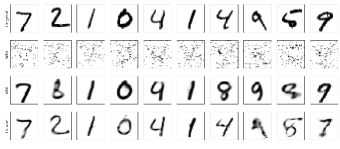
Figure 1: original images, reconstructions by BIHT, VAE and LS-VAE (from top to bottom row) with 100 measurements

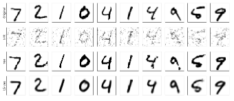
Figure 2: original images, reconstructions by BIHT, VAE and LS-VAE (from top to bottom row) with 300 measurements

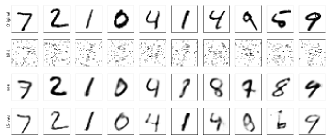
Figure 3: original images, reconstructions by BIHT, VAE and LS-VAE (from top to bottom row) with 100 measurements and 3% sign flips

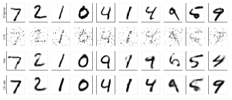
Figure 4: original images, reconstructions by BIHT, VAE and LS-VAE (from top to bottom row) with 300 measurements and 3% sign flips

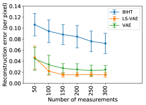
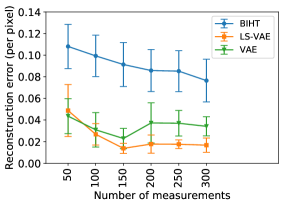
Figure 5: pixel-wise reconstruction error as the number of measurements varies. Error bars indicate 95% confidence intervals. The result with no sign flips and with 3% sign flips are shown in the left and right, respectively.

4 Conclusion

We present a least square decoder by exploring the low generative intrinsic dimension structure of the target for the 1-bit compressive sensing with possible sign-flips. Under the assumption that the target signals can be approximately generated via $L$-Lipschitz generator $G:\mathbb{R}^{k}\rightarrow\mathbb{R}^{n},k\ll n$, we prove that, up to a constant $c$, with high probability, the least square decoder achieves a sharp estimation error $\mathcal{O}(\sqrt{\frac{k\log(Ln)}{m}})$ as long as $m\geq O(k\log(Ln))$. We verify the (approximately) deep generative prior holds if the target signals have low intrinsic dimensions by constructing a ReLU network with properly chosen depth and width. Extensive numerical simulations and comparisons with state-of-the-art methods demonstrated the least square decoder is the robust to noise and sign flips, which verifies our theory. We only consider the analysis of the least squares decoders, we will leave the analysis of the regularized least squares decoder in the future work.

References

- [1] Mehmet Eren Ahsen and Mathukumalli Vidyasagar. An approach to one-bit compressed sensing based on probably approximately correct learning theory. The Journal of Machine Learning Research, 20(1):408–430, 2019.
- [2] Peter L Bartlett, Nick Harvey, Christopher Liaw, and Abbas Mehrabian. Nearly-tight vc-dimension and pseudodimension bounds for piecewise linear neural networks. J. Mach. Learn. Res., 20:63–1, 2019.
- [3] Peter L Bartlett, Vitaly Maiorov, and Ron Meir. Almost linear vc dimension bounds for piecewise polynomial networks. In Advances in neural information processing systems, pages 190–196, 1999.
- [4] Ashish Bora, Ajil Jalal, Eric Price, and Alexandros G Dimakis. Compressed sensing using generative models. In International Conference on Machine Learning, pages 537–546. PMLR, 2017.
- [5] Stéphane Boucheron, Gábor Lugosi, and Pascal Massart. Concentration inequalities: A nonasymptotic theory of independence. Oxford university press, 2013.
- [6] Petros T Boufounos. Greedy sparse signal reconstruction from sign measurements. In Signals, Systems and Computers, 2009 Conference Record of the Forty-Third Asilomar Conference on, pages 1305–1309. IEEE, 2009.
- [7] Petros T Boufounos and Richard G Baraniuk. 1-bit compressive sensing. In Information Sciences and Systems, 2008. CISS 2008. 42nd Annual Conference on, pages 16–21. IEEE, 2008.
- [8] David R Brillinger. A generalized linear model with gaussian regressor variables. A Festschrift For Erich L. Lehmann, page 97, 1982.
- [9] Emmanuel J. Candés, Justin Romberg, and Terence Tao. Robust uncertainty principles: Exact signal reconstruction from highly incomplete frequency information. IEEE Trans. Inform. Theory, 52(2):489–509, 2006.
- [10] Dao-Qing Dai, Lixin Shen, Yuesheng Xu, and Na Zhang. Noisy 1-bit compressive sensing: models and algorithms. Applied and Computational Harmonic Analysis, 40(1):1–32, 2016.
- [11] Zhao Ding, Junjun Huang, Yuling Jiao, Xiliang Lu, and Zhijian Yang. Robust decoding from binary measurements with cardinality constraint least squares. arXiv preprint arXiv:2006.02890, 2020.
- [12] David L. Donoho. Compressed sensing. IEEE Trans. Inform. Theory, 52(4):1289–1306, 2006.
- [13] Kenneth Falconer. Fractal geometry: mathematical foundations and applications. John Wiley & Sons, 2004.
- [14] M Fazel, E Candes, B Recht, and P Parrilo. Compressed sensing and robust recovery of low rank matrices. In Signals, Systems and Computers, 2008 42nd Asilomar Conference on, pages 1043–1047. IEEE, 2008.
- [15] Simon Foucart and Holger Rauhut. A mathematical introduction to compressive sensing, volume 1. Birkhäuser Basel, 2013.
- [16] Ian Goodfellow, Jean Pouget-Abadie, Mehdi Mirza, Bing Xu, David Warde-Farley, Sherjil Ozair, Aaron Courville, and Yoshua Bengio. Generative adversarial nets. In Advances in Neural Information Processing Systems 27, pages 2672–2680. Curran Associates, Inc., 2014.
- [17] Sivakant Gopi, Praneeth Netrapalli, Prateek Jain, and Aditya Nori. One-bit compressed sensing: Provable support and vector recovery. In International Conference on Machine Learning, pages 154–162, 2013.
- [18] Ankit Gupta, Robert Nowak, and Benjamin Recht. Sample complexity for 1-bit compressed sensing and sparse classification. In Information Theory Proceedings (ISIT), 2010 IEEE International Symposium on, pages 1553–1557. IEEE, 2010.
- [19] Paul Hand, Oscar Leong, and Vladislav Voroninski. Phase retrieval under a generative prior. arXiv preprint arXiv:1807.04261, 2018.
- [20] Jarvis Haupt and Richard Baraniuk. Robust support recovery using sparse compressive sensing matrices. In Information Sciences and Systems (CISS), 2011 45th Annual Conference on, pages 1–6. IEEE, 2011.
- [21] Jian Huang, Yuling Jiao, Zhen Li, Shiao Liu, Yang Wang, and Yunfei Yang. An error analysis of generative adversarial networks for learning distributions. arXiv preprint arXiv:2105.13010, 2021.
- [22] Jian Huang, Yuling Jiao, Xiliang Lu, and Liping Zhu. Robust decoding from 1-bit compressive sampling with ordinary and regularized least squares. SIAM Journal on Scientific Computing, 40(4):A2062–A2086, 2018.
- [23] Wen Huang, Paul Hand, Reinhard Heckel, and Vladislav Voroninski. A provably convergent scheme for compressive sensing under random generative priors. arXiv preprint arXiv:1812.04176, 2018.
- [24] Xiaolin Huang, Lei Shi, Ming Yan, and Johan AK Suykens. Pinball loss minimization for one-bit compressive sensing. arXiv preprint arXiv:1505.03898, 2015.
- [25] Laurent Jacques, Kévin Degraux, and Christophe De Vleeschouwer. Quantized iterative hard thresholding: Bridging 1-bit and high-resolution quantized compressed sensing. arXiv preprint arXiv:1305.1786, 2013.
- [26] Laurent Jacques, Jason N Laska, Petros T Boufounos, and Richard G Baraniuk. Robust 1-bit compressive sensing via binary stable embeddings of sparse vectors. IEEE Transactions on Information Theory, 59(4):2082–2102, 2013.
- [27] Diederik P Kingma and Max Welling. Auto-encoding variational bayes. In ICLR, 2014.
- [28] Jason N Laska and Richard G Baraniuk. Regime change: Bit-depth versus measurement-rate in compressive sensing. IEEE Transactions on Signal Processing, 60(7):3496–3505, 2012.
- [29] Jason N Laska, Zaiwen Wen, Wotao Yin, and Richard G Baraniuk. Trust, but verify: Fast and accurate signal recovery from 1-bit compressive measurements. IEEE Transactions on Signal Processing, 59(11):5289–5301, 2011.
- [30] Yann LeCun, Léon Bottou, Yoshua Bengio, and Patrick Haffner. Gradient-based learning applied to document recognition. Proceedings of the IEEE, 86(11):2278–2324, 1998.
- [31] Ker-Chau Li and Naihua Duan. Regression analysis under link violation. The Annals of Statistics, pages 1009–1052, 1989.
- [32] Wenhui Liu, Da Gong, and Zhiqiang Xu. One-bit compressed sensing by greedy algorithms. Numerical Mathematics: Theory, Methods and Applications, 9(2):169–184, 2016.
- [33] Zhaoqiang Liu, Selwyn Gomes, Avtansh Tiwari, and Jonathan Scarlett. Sample complexity bounds for 1-bit compressive sensing and binary stable embeddings with generative priors. In International Conference on Machine Learning, pages 6216–6225. PMLR, 2020.
- [34] Zhaoqiang Liu and Jonathan Scarlett. The generalized lasso with nonlinear observations and generative priors. Advances in Neural Information Processing Systems, 33, 2020.
- [35] Zhaoqiang Liu and Jonathan Scarlett. Information-theoretic lower bounds for compressive sensing with generative models. IEEE Journal on Selected Areas in Information Theory, 1(1):292–303, 2020.
- [36] Stephane Mallat. A wavelet tour of signal processing: the sparse way. Academic press, 2008.
- [37] Matey Neykov, Jun S Liu, and Tianxi Cai. L1-regularized least squares for support recovery of high dimensional single index models with gaussian designs. The Journal of Machine Learning Research, 17(1):2976–3012, 2016.
- [38] Yaniv Plan and Roman Vershynin. One-bit compressed sensing by linear programming. Communications on Pure and Applied Mathematics, 66(8):1275–1297, 2013.
- [39] Yaniv Plan and Roman Vershynin. Robust 1-bit compressed sensing and sparse logistic regression: A convex programming approach. IEEE Transactions on Information Theory, 59(1):482–494, 2013.
- [40] Yaniv Plan and Roman Vershynin. The generalized lasso with non-linear observations. IEEE Transactions on information theory, 62(3):1528–1537, 2016.
- [41] Yaniv Plan, Roman Vershynin, and Elena Yudovina. High-dimensional estimation with geometric constraints. Information and Inference: A Journal of the IMA, 6(1):1–40, 2017.
- [42] Shuang Qiu, Xiaohan Wei, and Zhuoran Yang. Robust one-bit recovery via relu generative networks: Near-optimal statistical rate and global landscape analysis. In International Conference on Machine Learning, pages 7857–7866. PMLR, 2020.
- [43] Danilo Jimenez Rezende and Shakir Mohamed. Variational inference with normalizing flows. In ICML, 2015.
- [44] Khalid Sayood. Introduction to data compression. Morgan Kaufmann, 2017.
- [45] Zuowei Shen, Haizhao Yang, and Shijun Zhang. Nonlinear approximation via compositions. Neural Networks, 119:74–84, 2019.
- [46] Dmitry Ulyanov, Andrea Vedaldi, and Victor Lempitsky. Deep image prior. In Proceedings of the IEEE conference on computer vision and pattern recognition, pages 9446–9454, 2018.
- [47] Gal Vardi, Gilad Yehudai, and Ohad Shamir. On the optimal memorization power of relu neural networks. arXiv preprint arXiv:2110.03187, 2021.
- [48] Santosh S Vempala. The random projection method, volume 65. American Mathematical Soc., 2005.
- [49] Roman Vershynin. Estimation in high dimensions: a geometric perspective. In Sampling theory, a renaissance, pages 3–66. Springer, 2015.
- [50] Roman Vershynin. High-dimensional probability: An introduction with applications in data science, volume 47. Cambridge university press, 2018.
- [51] Roman Vershynin. Memory capacity of neural networks with threshold and rectified linear unit activations. SIAM Journal on Mathematics of Data Science, 2(4):1004–1033, 2020.
- [52] Xiaohan Wei, Zhuoran Yang, and Zhaoran Wang. On the statistical rate of nonlinear recovery in generative models with heavy-tailed data. In International Conference on Machine Learning, pages 6697–6706. PMLR, 2019.
- [53] Yan Wu, Mihaela Rosca, and Timothy Lillicrap. Deep compressed sensing. In International Conference on Machine Learning, pages 6850–6860. PMLR, 2019.
- [54] Ming Yan, Yi Yang, and Stanley Osher. Robust 1-bit compressive sensing using adaptive outlier pursuit. IEEE Transactions on Signal Processing, 60(7):3868–3875, 2012.
- [55] Lijun Zhang, Jinfeng Yi, and Rong Jin. Efficient algorithms for robust one-bit compressive sensing. In International Conference on Machine Learning, pages 820–828, 2014.
- [56] Argyrios Zymnis, Stephen Boyd, and Emmanuel Candes. Compressed sensing with quantized measurements. IEEE Signal Processing Letters, 17(2):149–152, 2010.