Spinning gauged boson and Dirac stars:
a comparative study

Abstract

Scalar boson stars and Dirac stars are solitonic solutions of the Einstein–Klein-Gordon and Einstein-Dirac classical equations, respectively. Despite the different bosonic $vs.$ fermionic nature of the matter field, these solutions to the classical field equations have been shown to have qualitatively similar features [1]. In particular, for spinning stars the most fundamental configurations can be in both cases toroidal, unlike spinning Proca stars that are spheroidal [2]. In this paper we gauge the scalar and Dirac fields, by minimally coupling them to standard electromagnetism. We explore the impact of the gauge coupling on the resulting solutions. One of the most relevant difference concerns the gyromagnetic ratio, which for the scalar stars takes values around 1, whereas for Dirac stars takes values around 2.

1 Introduction and motivation

In a recent paper [2], we have performed a comparative analysis of the spinning solitons arising in the Einstein-Klein-Gordon, Einstein-Dirac and Einstein-Proca models. Using numerical methods, particle-like solutions were found and their basic properties analysed. This analysis has indicated a, a priori non-obvious, high degree of universality between the different models, and in particular with some features holding for both bosonic and Dirac stars. Amongst these, we have noticed that both scalar and Dirac stars can present a distinctive toroidal morphology, contrasting with the spheroidal morphology of Proca stars [2].

Bosonic stars (scalar or vector) can in principle be macroscopic objects, corresponding to many bosons in the same quantum state, to justify the classical description. In fact these models have been widely considered in astrophysical contexts, for instance as black hole mimickers - see $e.g.$ [4, 3] for some recent discussions. The status of Dirac stars is less clear. Still, one may entertain the possibility that both models could be an approximate description for microscopic objects, eventually relevant in the early Universe. In such context, a differentiated phenomenology could arise, $e.g.$ from their interaction with electromagnetic fields.

With this physical motivation, besides the intrinsic interest in understanding self-gravitating solitons in simple physical models, in this paper we extend the results in [1] to the case of gauged matter fields. We shall focus on the scalar and Dirac cases, and consider the Einstein–Klein-Gordon and Einstein–Dirac equations minimally coupled to an electromagnetic field. We shall construct the electrically charged, spinning particle-like solutions, which generalize the neutral solitons in [2], and describe some of their properties, in particular their gyromagnetic ratio.

Static, spherically symmetric neutral scalar ($s=0$) boson stars have been known for more than half a century [5, 6]. Their gauged generalization, on the other hand, were only discussed for the first time in [7], and more recently in [8]. Moreover, spinning boson stars were first constructed in [9, 10] for free and in [11, 12] for self-interacting (with a $Q$-ball type potential) complex scalar fields. Finally, spinning gauged boson stars have also been constructed for free [13] and self-interacting (with a $Q$-ball type potential) complex scalar fields [14, 15].

Spherical, neutral Dirac ($s=1/2$) stars were first constructed in [17] and their gauged version in [18]. The latter are solutions of the Einstein-Maxwell-Dirac equations with two gauged fermions, with opposite spins, in order to satisfy spherical symmetry. Thus, both the neutral and the charged spherical solutions require at least two Dirac fields. Solutions with a single Dirac field were constructed as spinning (neutral) solutions in [2] for the first time, in a model that, therefore, does not admit static stars. So far, no construction of spinning gauged Dirac stars has appeared in the literature.

The solutions reported below - the gauged generalizations of the spinning solitons with $s=0,1/2$ in [2] - possess a nonzero ADM mass, electric charge and a magnetic dipole moment, similarly to the well known Kerr-Newman black hole of electrovacuum. The latter has a gyromagnetic ratio of $g=2$ [19] so one may inquire about the gyromagnetic ratio of these solutions, which is an important quantity in particle physics. Indeed, the experimental value of the quantity $g-2$, which is known with an incredible accuracy, is a very precise test of the Standard Model and possible deviations from the theoretical value may be a smoking gun for new physics. In fact, the recently discussed possible disagreement between theory and experiment for $(g-2)_{\rm muon}$ is one of the most hotly debated topics in the particle physics community [20]. It has also been suggested that strong gravitational interaction may also play an important role in very precise calculations of the corrections to the gyromagnetic ratio [21, 22, 23, 24]. Concerning the solitons discussed herein, as we shall see there is a clear quantitative difference between $g$ for scalar and Dirac gauged spinning stars.

This paper is organized as follows. In Section 2 we exhibit the models, discuss their equations of motion, relevant physical quantities and the Ansatze that will be used to computed spinning gauged scalar and Dirac stars. Section 3 discusses the boundary conditions and the numerical method to obtain the solutions; then, the numerical results are presented. Besides the discussion on $g$, we find, for instance, that in both cases, the proportionality relation found in [2] between the angular momentum and the Noether charge (particle number) still holds. Moreover, the ratio between the electric charge and the Noether charge is equal to the gauge coupling constant. In fact, some basic features are similar to those of the ungauged stars. In particular, for a given value of the gauge coupling constant $q$, one finds again a limited range for the allowed frequencies of the matter fields, which is bounded from above by the fields’ mass and from below by a minimal frequency whose value decreases with $q$. Finally, in Section 4 we provide a discussion of the results and some final remarks.

2 The general framework

2.1 The models and field equations

We consider Einstein’s gravity in 3+1 dimensions minimally coupled with a spin-$s$ field ($s=0,1/2$) :

$$\mathcal{S}=\frac{1}{4\pi}\int d^{4}x\sqrt{-g}\left[\frac{R}{4G}-\frac{1}{4}F^{2}+\mathcal{L}_{(s)}\right]\ .$$ (2.1)

The notation and conventions used here follow closely those in [1, 2, 25]: $G$ is the gravitational constant, $R$ is the Ricci scalar associated with the spacetime metric $g_{\mu\nu}$, $F_{\mu\nu}=\partial_{\mu}A_{\nu}-\partial_{\nu}A_{\mu}$ is the $U(1)$ field strength tensor. For the matter Lagrangian $\mathcal{L}_{(s)}$ we consider two cases:

$$\mathcal{L}_{(0)}=-\frac{1}{2}g^{\alpha\beta}\left[(D_{\alpha}\Phi)^{*}D_{\beta}\Phi+(D_{\beta}\Phi)^{*}D_{\alpha}\Phi\right]-\mu^{2}\Phi^{*}\Phi\ ,~{}~{}{\rm with}~{}~{}D_{\nu}\Phi=(\partial_{\nu}+iqA_{\nu})\Phi,$$ (2.2)

$$\mathcal{L}_{(1/2)}=-i\left[\frac{1}{2}\left(\{\hat{\not{D}}\overline{\Psi}\}\Psi-\overline{\Psi}\hat{\not{D}}\Psi\right)+\mu\overline{\Psi}\Psi\right]\ ,~{}~{}{\rm with}~{}~{}\hat{D}_{\nu}\Psi=(\partial_{\nu}-\Gamma_{\nu}+iqA_{\nu})\Psi~{}.$$ (2.3)

Here, $\Phi$ is a complex scalar field; $\Psi$ is a Dirac spinor, with four complex components. For the scalar field, the asterisk denotes complex conjugation; $\overline{\Psi}$ denotes the Dirac conjugate [27]. $\hat{\not{D}}\equiv\gamma^{\mu}\hat{D}_{\mu}$, where $\gamma^{\mu}$ are the curved spacetime gamma matrices, and $\Gamma_{\mu}$ are the spinor connection matrices [27]. In both cases, $\mu>0$ corresponds to the mass of the field(s), while $q$ is the gauge coupling constant.

Variation of (2.1) with respect to the metric leads to the Einstein field equations

$$G_{\alpha\beta}=2G~{}T_{\alpha\beta}\qquad{\rm with}\qquad T_{\alpha\beta}=T_{\alpha\beta}^{(M)}+T_{\alpha\beta}^{(s)}\ ,$$ (2.4)

where $G_{\alpha\beta}$ is the Einstein tensor and the pieces of the stress-energy tensor are

$$T_{\alpha\beta}^{(M)}=F_{\alpha\gamma}F_{\beta\delta}g^{\gamma\delta}-\frac{1}{4}g_{\alpha\beta}F^{2}\ ,$$ (2.5)

for the Maxwell field, and the following $T_{\alpha\beta}^{(s)}$ for the (gauged) scalar and Dirac fields, respectively:

$$T_{\alpha\beta}^{(0)}=(D_{\alpha}\Phi)^{*}D_{\beta}\Phi+(D_{\beta}\Phi)^{*}D_{\alpha}\Phi-g_{\alpha\beta}\left[\frac{1}{2}g^{\gamma\delta}((D_{\gamma}\Phi)^{*}D_{\delta}\Phi+(D_{\delta}\Phi)^{*}D_{\gamma}\Phi)+\mu^{2}\Phi^{*}\Phi\right]\ ,$$ (2.6)

$$T_{\alpha\beta}^{(1/2)}=-\frac{i}{2}\left[\overline{\Psi}\gamma_{(\alpha}\hat{D}_{\beta)}\Psi-\left\{\hat{D}_{(\alpha}\overline{\Psi}\right\}\,\gamma_{\beta)}\Psi\right]\ .$$ (2.7)

The corresponding matter field equations are:

$$D_{\nu}D^{\nu}\Phi-\mu^{2}\Phi=0~{}~{}(s=0)\ ,\qquad(\gamma^{\nu}\hat{D}_{\nu}-\mu)\Psi=0~{}~{}(s=1/2)\ ,~{}~{}$$ (2.8)

and

$$\nabla_{\alpha}\mathcal{F}^{\alpha\beta}=qJ^{\beta}\ ,~{}~{}{\rm with}~{}~{}J^{\beta}=iq\big{[}(D^{\beta}\Phi^{*})\Phi-\Phi^{*}(D^{\beta}\Phi)\big{]}~{}~{}~{}(s=0)\ ,\quad{\rm or}\quad~{}J^{\beta}=\overline{\Psi}\gamma^{\beta}\Psi~{}~{}~{}(s=1/2).$$ (2.9)

for the Maxwell field.

These models are invariant under the $local$ $U(1)$ gauge transformation

$$(\Phi\to\Phi e^{-iq\alpha},~{}~{}\Psi\to\Psi e^{-iq\alpha}),~{}~{}{\rm and}~{}~{}A_{\mu}\to A_{\mu}+\partial_{\mu}\alpha,$$ (2.10)

with $\alpha$ a real function of spacetime coordinates. The current and the total energy-momentum tensor are covariantly conserved,

$$\nabla_{\mu}J^{\mu}=0\ ,\qquad\nabla_{\mu}T^{\mu\nu}=0\ .$$ (2.11)

Then, integrating the timelike component of the 4-current $J^{\mu}$ on a spacelike hypersurface $\Sigma$ yields a conserved Noether charge (particle number):

$$Q=\int_{\Sigma}~{}J^{t}\ .$$ (2.12)

2.2 The Ansatz

The employed metric Ansatz is similar to that used in the ungauged case [2], with a line-element possessing two Killing vectors $\partial_{\varphi}$ and $\partial_{t}$ (with $\varphi$ and $t$ the azimuthal and time coordinate, respectively):

$$ds^{2}=-e^{2F_{0}}dt^{2}+e^{2F_{1}}\left(dr^{2}+r^{2}d\theta^{2}\right)+e^{2F_{2}}r^{2}\sin^{2}\theta\left(d\varphi-\frac{W}{r}dt\right)^{2}\ .$$ (2.13)

This metric contains four functions $(F_{i};W)$, $i=0,1,2$, which depend on the spherical coordinates $r$ and $\theta$ only. The Minkowski spacetime background is approached for $r\to\infty$, where the asymptotic values are $F_{i}=0$, $W=0$.

In the scalar case, one the following Ansatz in terms of a single real function $\phi(r,\theta)$ and a complex phase ($\varphi,t$), with

$$\Phi=e^{i(m\varphi-wt)}\phi(r,\theta)\ .$$ (2.14)

In the case of a Dirac field, the Ansatz contains two complex functions [2]:

$$\Psi=e^{i(m\varphi-wt)}\begin{pmatrix}\psi_{1}(r,\theta)\\ \psi_{2}(r,\theta)\\ -i\psi_{1}^{*}(r,\theta)\\ -i\psi_{2}^{*}(r,\theta)\end{pmatrix}\ ,~{}~{}{\rm with}~{}~{}\psi_{1}(r,\theta)=P(r,\theta)+i\mathcal{Q}(r,\theta)\ ,~{}~{}\psi_{2}(r,\theta)=X(r,\theta)+iY(r,\theta)\ .$$ (2.15)

We shall employ the following orthonormal tetrad, as implied from the metric form (2.13)

$${\bf e}^{0}_{\mu}dx^{\mu}=e^{F_{0}}dt\ ,\qquad{\bf e}^{1}_{\mu}dx^{\mu}=e^{F_{1}}dr\ ,\qquad{\bf e}^{2}_{\mu}dx^{\mu}=e^{F_{1}}rd\theta\ ,\qquad{\bf e}^{3}_{\mu}dx^{\mu}=e^{F_{2}}r\sin\theta\left(d\varphi-\frac{W}{r}dt\right)\ ,$$ (2.16)

such that $ds^{2}=\eta_{ab}({\bf e}^{a}_{\mu}dx^{\mu})({\bf e}^{b}_{\nu}dx^{\nu})$, where $\eta_{ab}={\rm diag}(-1,+1,+1,+1)$.

For a scalar field, the parameter $m$ in an integer, while for the Dirac field $m$ is a half-integer; $w$ is the field’s frequency in both cases, which we shall take to be positive. A study of each of the matter field equations in the far field reveals that the solutions satisfy the bound state condition $w<\mu$.

The Ansatz for the $U(1)$ potential contains two real functions – an electric and a magnetic potential, with:

$$A=A_{\mu}dx^{\mu}=V(r,\theta)dt+A_{\varphi}(r,\theta)r\sin\theta d\varphi\ .$$ (2.17)

Note that, in contrast to the ungauged case, the $(t,\varphi)$-dependence of the scalar field $\psi$ can now be gauged away by applying the local $U(1)$ symmetry (2.10) with $\alpha=(m\varphi-\omega t)/q$. However, this would also change the gauge field as $V\to V-\omega/q$, $A_{\varphi}\to A_{\varphi}+m/q$, so that it would (formally) become singular in the $q\to 0$ limit. Therefore, in order to be able to consider this limit, we prefer to keep the $(t,\varphi)$-dependence in the Ansatz and to fix the corresponding gauge freedom by setting $V=A_{\varphi}=0$ at infinity.

2.3 Quantities of interest

Given the above general Ansatz, the computation of the explicit form of the field equations is straightforward. Although the resulting expressions are in general too complicated to include here, the angular momentum density is simple enough, with

$$(T^{(0)})_{\varphi}^{t}=2e^{-2F_{0}}(m+qA_{\varphi}r\sin\theta)\left(w-qV-(m+qA_{\varphi}r\sin\theta)\frac{W}{r}\right)\phi^{2}\ ,$$ (2.18)

$$(T^{(1/2)})_{\varphi}^{t}=e^{-F_{0}}(m+qA_{\varphi}r\sin\theta)(P^{2}+\mathcal{Q}^{2}+X^{2}+Y^{2})+e^{-F_{0}-F_{1}+F_{2}}\sin\theta\left\{(PX+\mathcal{Q}Y)[1+r(F_{2,r}-F_{0,r})]\right.$$ (2.19)

$${~{}~{}~{}~{}~{}}\left.-\frac{1}{2}(P^{2}+\mathcal{Q}^{2}-X^{2}-Y^{2})(\cot\theta+F_{2,\theta}-F_{0,\theta})+2e^{-F_{0}+F_{1}}r\left(w-qV-(m+qA_{\varphi}r\sin\theta)\frac{W}{r}\right)(\mathcal{Q}X-PY)\right\}\ ,$$

$$(T^{(M)})_{\varphi}^{t}=-\frac{e^{-2(F_{0}+F_{1})}}{r}\bigg{[}\sin\theta(r^{2}A_{\varphi,r}V_{,r}+A_{\varphi,\theta}V_{,\theta})+\sin^{2}\theta W(r^{2}A_{\varphi,r}^{2}+A_{\varphi,\theta}^{2})$$ (2.20)

$${~{}~{}~{}~{}~{}~{}~{}~{}~{}~{}}+A_{\varphi}\bigg{(}r\sin\theta V_{,r}+\cos\theta V_{,\theta}+W\left(A_{\varphi}+2\sin\theta(r\sin\theta A_{\varphi,r}+\cos\theta A_{\varphi,\theta})\right)\bigg{)}\bigg{]}\ .$$

Observe the presence of a $U(1)$-contribution in $(T^{(s)})_{\varphi}^{t}$. Of interest is also the temporal component of the current density:

$$J^{t}_{(0)}=2e^{-2F_{0}}\left(w-qV-(m+qA_{\varphi}r\sin\theta)\frac{W}{r}\right)\phi^{2}\ ,$$ (2.21)

$$J^{t}_{(1/2)}=2e^{-F_{0}}(P^{2}+\mathcal{Q}^{2}+X^{2}+Y^{2})\ .$$ (2.22)

The ADM mass $M$ and the angular momentum $J$ of the solutions are read off from the asymptotic expansion:

$$g_{tt}=-1+\frac{2M}{r}+\dots\ ,\qquad g_{\varphi t}=-\frac{2J}{r}\sin^{2}\theta+\dots\ .\ \ \$$ (2.23)

Of interest is also the asymptotic decay of the gauge field

$$V\sim\frac{Q_{e}}{r}+\dots~{},~{}~{}~{}\qquad A_{\varphi}\sim\frac{\mu_{m}\sin\theta}{r^{2}}+\dots\ ,$$ (2.24)

where $Q_{e}$ and $\mu_{m}$ are the electric charge and the magnetic dipole moment, respectively.

The total angular momentum can also be computed as the integral of the corresponding density

$$J=2\pi\int^{\infty}_{0}dr\,\int^{\infty}_{0}d\theta r^{2}e^{F_{0}+2F_{1}+F_{2}}\left((T^{(s)})_{\varphi}^{t}+(T^{(M)})_{\varphi}^{t}\right)\ .$$ (2.25)

The explicit form of the Noether charge, as computed from (2.12), is

$$Q\equiv Q_{(s)}=2\pi\int^{\infty}_{0}dr\,\int^{\infty}_{0}d\theta r^{2}e^{F_{0}+2F_{1}+F_{2}}j^{t}_{(s)}\ .$$ (2.26)

For both a scalar field and a Dirac one, a straightforward computation shows that $J$, $Q$ and $Q_{e}$ are proportional,

$$J=mQ=\frac{mQ_{e}}{q}\ .$$ (2.27)

Note that the above relation is nontrivial, since the angular momentum density and Noether charge density are $not$ proportional. Nonetheless, the proportionality still holds at the level of the integrated quantities.

As with any spinning system with gauge fields, the solutions possess also a non-zero gyromagnetic ratio $g$, which defines how the magnetic dipole moment is induced by the total angular momentum and charge, for a given total mass:

$$\mu_{m}=g\frac{Q_{e}}{2M}J\ .$$ (2.28)

3 The solutions

3.1 The boundary conditions and numerical method

The numerical treatment of the problem is simplified by using some symmetries of the equations of motion [1]. Firstly, the factor of $G$ in the Einstein field equations is set to unity by a redefinition of the matter functions,

$$\{\Phi,\Psi,A\}\to\frac{1}{\sqrt{G}}\{\Phi,\Psi,A\}\ .$$ (3.29)

Secondly, one sets $\mu=1$ in the equations. This can be done without any loss of generality, by noticing that the field equations remain invariant under the transformation

$$r\to\lambda r;~{}~{}~{}~{}W\to\lambda W,~{}F_{i}\to F_{i};~{}~{}~{}\{w,\mu,q\}\to\frac{1}{\lambda}\{w,\mu,q\}\ ;\ \ \ \left\{\begin{array}[]{l}\displaystyle{\Phi\to\Phi}\\ \Psi\to\frac{1}{\sqrt{\lambda}}\Psi\\ A\to A\end{array}\right\},$$ (3.30)

where $\lambda$ is a positive constant. As for some quantities of interest, they transform as

$$M\to\lambda M,~{}~{}J\to\lambda^{2}J,~{}~{}Q_{e}\to\lambda Q_{e},~{}~{}Q\to\lambda^{2}Q~{}~{}{\rm and}~{}~{}\mu_{m}\to\lambda\mu_{m}\ .$$ (3.31)

This invariance is used to do the numerical work in units set by the field’s mass, $i.e.$ one takes $\lambda={1}/{\mu}$. Let us remark that only quantities which are invariant under the transformation (3.30) (like $w/\mu$, $q/\mu$, $J/M^{2}$ or $M\mu$) are relevant.

Given the Ansatz (2.14), (2.15), (2.17), all components of the energy momentum tensor are zero, except for $T_{rr},~{}T_{r\theta},~{}T_{\varphi\varphi},~{}T_{tt}$ and $T_{\varphi t}$, which possess a $(r,\theta)$-dependence only (although the scalar and spinor fields are $not$ time independent).

Then, the Einstein field equations with the energy momentum-tensors (2.5), (2.6), (2.7), plus the matter field equations (2.8), (2.9) together with the Ansatz (2.13) (2.14), (2.15), (2.17), lead to a system of seven (ten) coupled partial differential equations for the gauged scalar (Dirac) models. There are four equations for the metric functions $F_{i},W$; together with three (six) equations for the matter functions. Apart from these, there are two constraint Einstein equations which are not solved in practice, being used the monitor the accuracy of the numerical results.

The boundary conditions are found by considering an approximate construction of the solutions on the boundary of the domain of integration together with the assumption of regularity and asymptotic flatness. The metric functions are subject to the following boundary conditions:

$$\partial_{r}F_{i}\big{|}_{r=0}=W\big{|}_{r=0}=0\ ,\qquad F_{i}\big{|}_{r=\infty}=W\big{|}_{r=\infty}=0\ ,\qquad\partial_{\theta}F_{i}\big{|}_{\theta=0,\pi}=\partial_{\theta}W\big{|}_{\theta=0,\pi}=0\ .$$ (3.32)

The scalar field amplitude vanishes on the boundary of the domain of integration,

$$\phi\big{|}_{r=0}=\phi\big{|}_{r=\infty}=\phi\big{|}_{\theta=0,\pi}=0\ .$$ (3.33)

For a Dirac field, all solutions considered so far have $m=1/2$, and satisfy the following boundary conditions

$$P\big{|}_{r=0}=\mathcal{Q}\big{|}_{r=0}=X\big{|}_{r=0}=Y\big{|}_{r=0}=0\ ,\qquad P\big{|}_{r=\infty}=\mathcal{Q}\big{|}_{r=\infty}=X\big{|}_{r=\infty}=Y\big{|}_{r=\infty}=0\ ,$$ (3.34)

$$\partial_{\theta}P\big{|}_{\theta=0}=\partial_{\theta}\mathcal{Q}\big{|}_{\theta=0}=X\big{|}_{\theta=0}=Y\big{|}_{\theta=0}=0\ ,\qquad P\big{|}_{\theta=\pi}=\mathcal{Q}\big{|}_{\theta=\pi}=\partial_{\theta}X\big{|}_{\theta=\pi}=\partial_{\theta}Y\big{|}_{\theta=\pi}=0\ .$$

Finally, for both $s=0,1/2$, the Maxwell potentials satisfy the boundary conditions:

$$\partial_{r}V\big{|}_{r=0}=A_{\varphi}\big{|}_{r=0}=0\ ,\qquad V\big{|}_{r=\infty}=A_{\varphi}\big{|}_{r=\infty}=0\ ,\qquad\partial_{\theta}V\big{|}_{\theta=0,\pi}=\partial_{\theta}A_{\varphi}\big{|}_{\theta=0,\pi}=0\ .$$ (3.35)

After setting $\mu=1$, the problem has still three input parameters: $\{w,m;q\}$ – the field frequency, the azimuthal number and the gauge coupling constant. The reported results in this work have $m=1$ for the scalar field and $m=1/2$ for a Dirac one.

The solutions are found by using a fourth order finite difference scheme. The system of seven/ten equations is discretised on a grid with $N_{r}\times N_{\theta}$ points; typically $N_{r}\sim 200$, $N_{\theta}\sim 50$. We introduce a new radial coordinate $x={r}/({r+c})$, which maps the semi-infinite region $[0,\infty)$ onto the unit interval $[0,1]$, where $c$ is a constant of order one.

The gauged boson stars were constructed by using the professional package FIDISOL/CADSOL [32] which uses a Newton-Raphson method. The Einstein-Dirac-Maxwell equations is solved with the Intel MKL PARDISO sparse direct solver [33], and using the CESDSOL library. In all cases, the typical errors are of order of $10^{-4}$.

Finally, we remark that the solutions shown here are fundamental states, with all matter functions being nodeless. However, we predict the existence of a discrete set of solutions, indexed by the number of nodes, $n$, of (some of) the matter function(s).

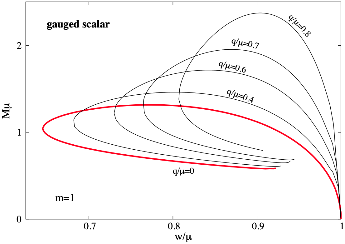
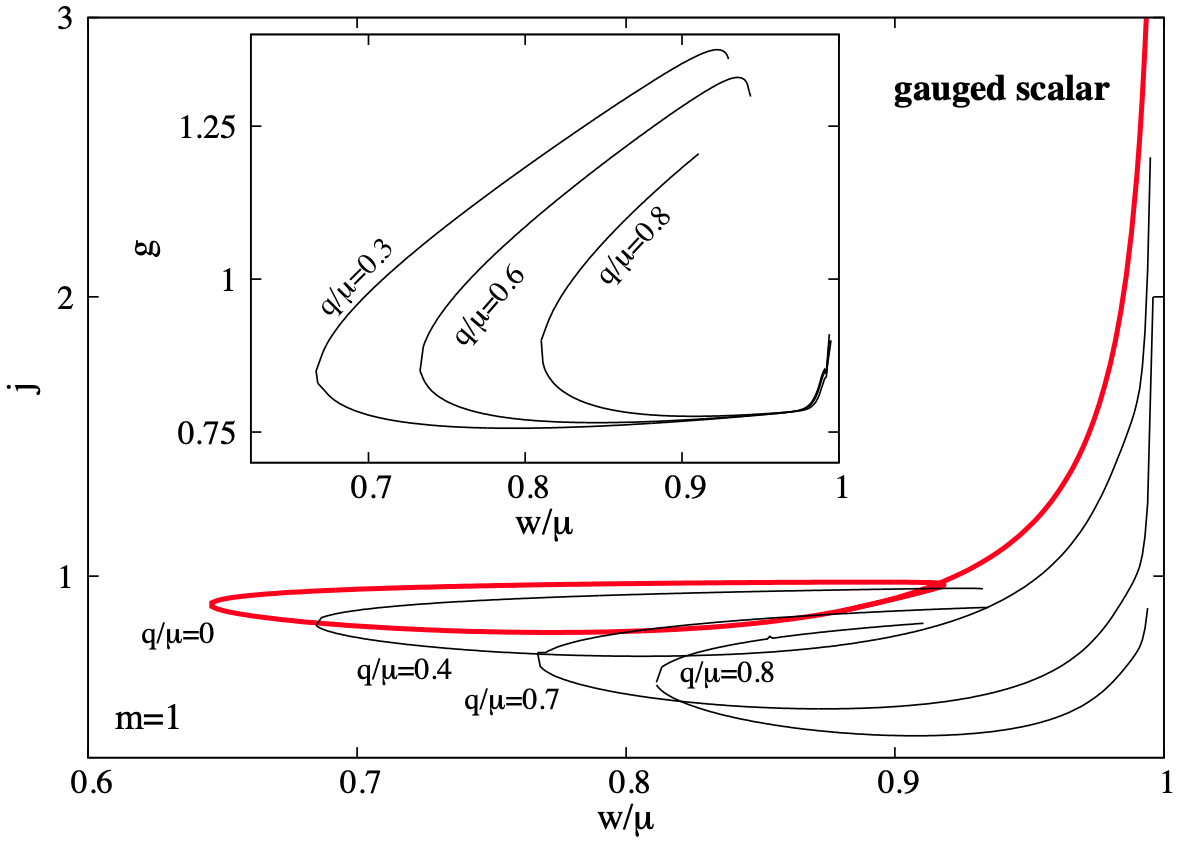
Figure 1: The ADM mass $M$ (left panel) and the reduced angular momentum $j=J/M^{2}$ and the gyromagnetic ratio $g$ (right panel) are shown for the families of spinning gauged boson stars with illustrative value of the gauged coupled constant $q$. The quantities are given in units set by the field mass $\mu$.

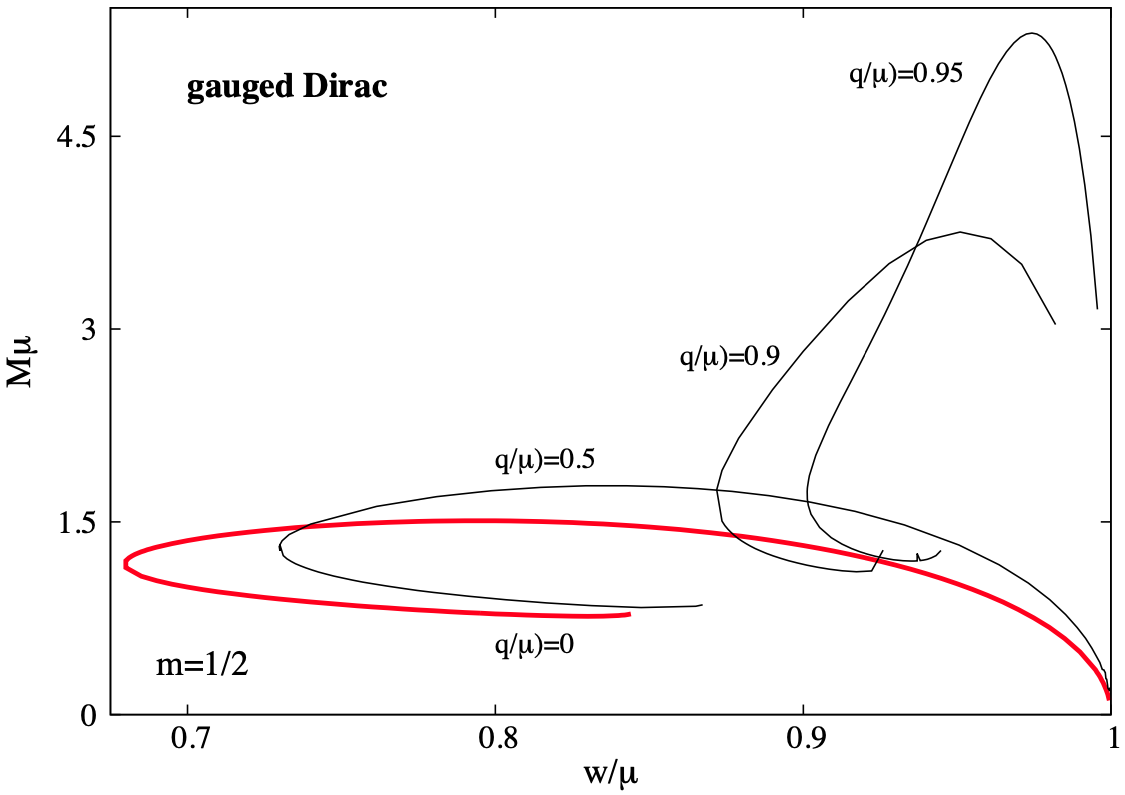
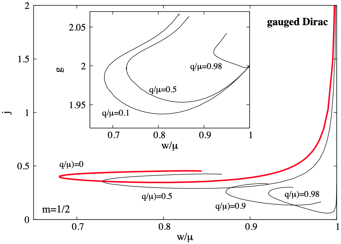
Figure 2: Same as Figure 1 for spinning gauged Dirac stars.

3.2 Numerical results

In our approach, we start with the ungauged solution in [2] ($i.e$ $q=0$ and $A_{\varphi}=V=0$). Then one can smoothly turn on the gauge field by increasing (from zero) the value of the gauge coupling constant $q$, while keeping fixed the other input constants (in particular the parameters $w,m$). The basic properties of the gravitating spinning gauged boson and Dirac stars solutions so constructed can be summarized as follows:

For a given values of $w$, spinning solutions appear to exist up to a maximal value of the gauge coupling constant only, $q_{\rm max}$, where the numerical process stops to converge. We remark that all global charges stay finite in that limit. The physical mechanism behind this behaviour is likely similar to that discussed for the spherically symmetric case [7, 18]: the electric charge repulsion becomes too strong and localized solutions cease to exist. A precise determination of $q_{\rm max}$ is challenging; all solutions found so far have $q/\mu<1$.

Given a value of $q$, the full spectrum of solutions is constructed by varying the field frequency $w$. The gauged spinning stars exist for a limited range of frequencies $0<w_{\rm min}<w<w_{\rm max}=\mu$, see Figs 1, 2. Observe that the minimal frequency increases with $q$.

A backbending towards larger values of $w$ is observed as $w\to w_{min}$, for both $s=0,1.2$. One may expect that, similar to the spherically symmetric case, this backbending would lead to an inspiraling of the solutions towards a limiting configuration with $w_{c}>w_{\rm min}$. However, the construction of these secondary branched is a complicated numerical task, which we do not attempt in this work. Also, the numerical accuracy decreases as $w/\mu\to 1$, with a delocalization of the profiles for the scalar and spinor functions, a different approach being necessary for the study of this limit.

As seen in Figures 1, 2. for any $q$, the $(w,M)$ looks qualitatively similar to that found in the ungauged case ($q=0$). The observed trend is that the maximal value of $M$ increases with $q$. Note that a similar behaviour is found for the $(w,J)$-dependence. Also, the minimal value of the reduced angular momentum $j=J/M^{2}$ decreases with $q$.

The shape of the metric functions and of the $s=0,1/2$ matter functions is rather similar to the ungauged case. Concerning the gauge field, the electric potential $V$ does not possess a strong angular dependence; however, the magnetic potential $A_{\varphi}$ exhibits an involved angular dependence.

Also, as seen in Figure 3 the energy density $-T_{t}^{t}$ of the $s=0$ solutions is localized in a finite region in the equatorial plane and decreases monotonically along the symmetry axis, such that the typical energy density isosurfaces have a toroidal shape. At the same time, the angular momentum density (which equals the Noether charge density) has a strong peak in the equatorial plane. Note that while $T_{\varphi}^{t}$ vanishes on the symmetry axis, this is not the case for $T_{t}^{t}$. The energy density distribution is still toroidal for typical Dirac stars, although becoming more spheroidal than in the scalar case - see Figure 4.

The gyromagnetic ratio $g$ of the solutions has a nontrivial dependence on both frequency and gauge coupling constant, taking values around 1 (for $s=0$ stars) and 2 for (for $s=1/2$ stars), the larger deviations being found along the secondary branches of solutions (see the insets in Figures 1, 2, right panels). Interestingly, the extrapolation of the numerical results towards the Newtonian limit $w/\mu\rightarrow 1$ suggest that $g\to 1$ $(s=0)$ and $g\to 2$ $(s=1/2$), independently of the value of the gauge coupling constant $q$.

It is also of interest to study the strong energy condition

$$\chi=\left(T_{\mu\nu}-\frac{1}{2}Tg_{\mu\nu}\right)X^{\mu}X^{\nu}\geq 0$$ (3.36)

(with the timelike vector $X^{\mu}$, $X^{\mu}X_{\mu}=-1$). We have monitored this condition for a number of solutions and have found that $\chi>0$ in all cases (see Figure (5) where this quantity is shown for the same configurations as in Figures (3), (4)).

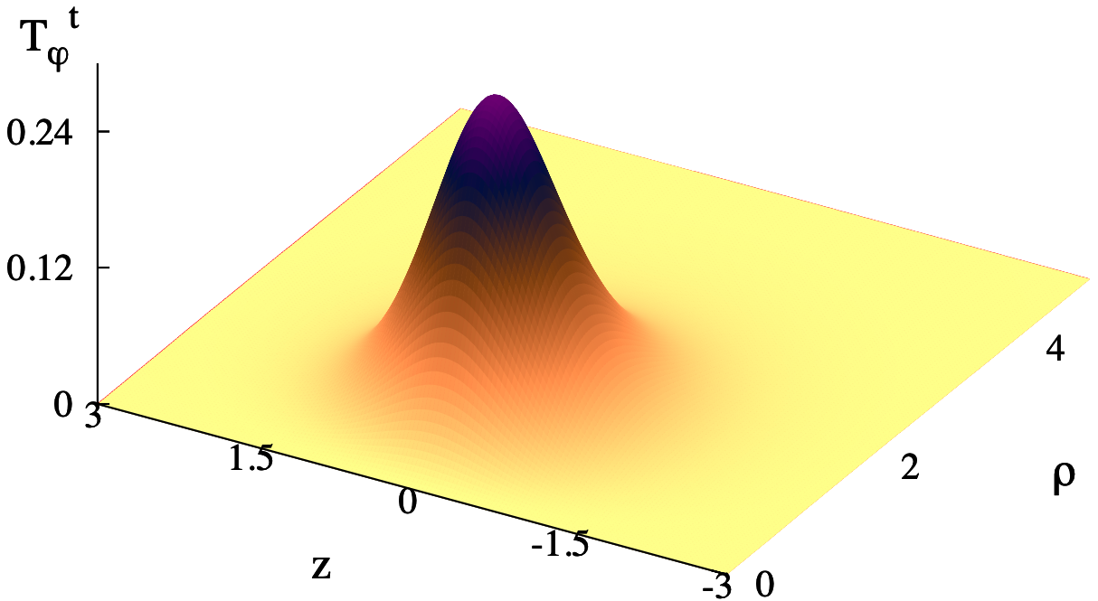
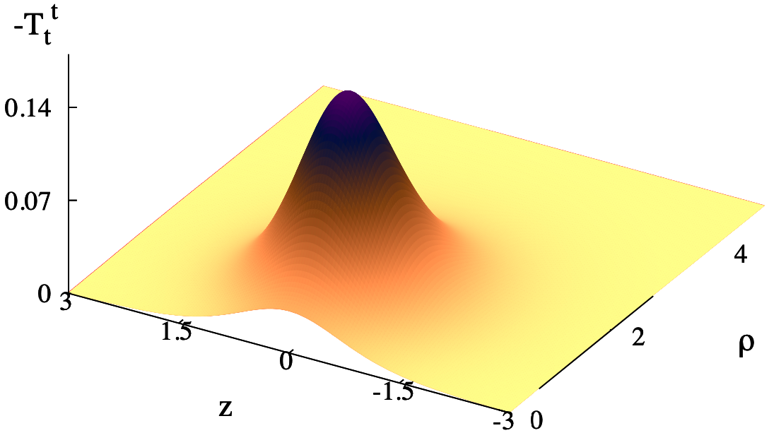
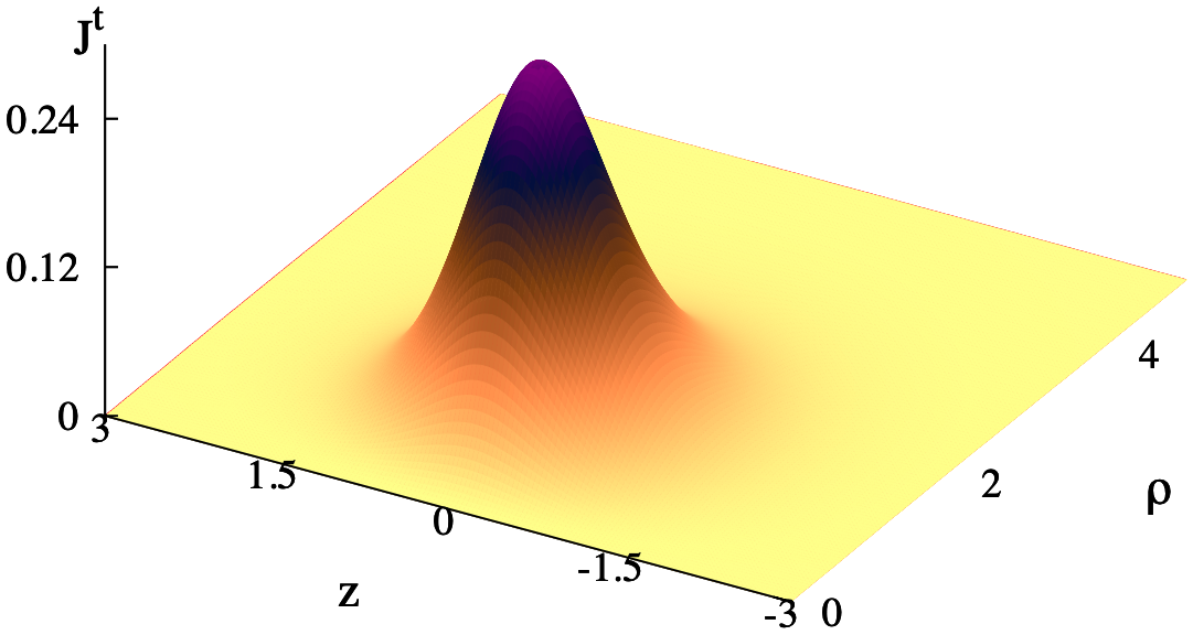
Figure 3: The components $T_{\varphi}^{t}$ and $T_{t}^{t}$ of the total energy momentum tensor, associated with angular momentum and energy densities and the $J^{t}$-component of the current are shown as a function of the cylindrical coordinates $(\rho,z)$ (with $\rho=r\sin\theta$, $z=r\cos\theta$) for a typical spinning gauged boson star. The input parameters are $m=1$, $w=0.75$, $\mu=1$ and $q=0.5$.

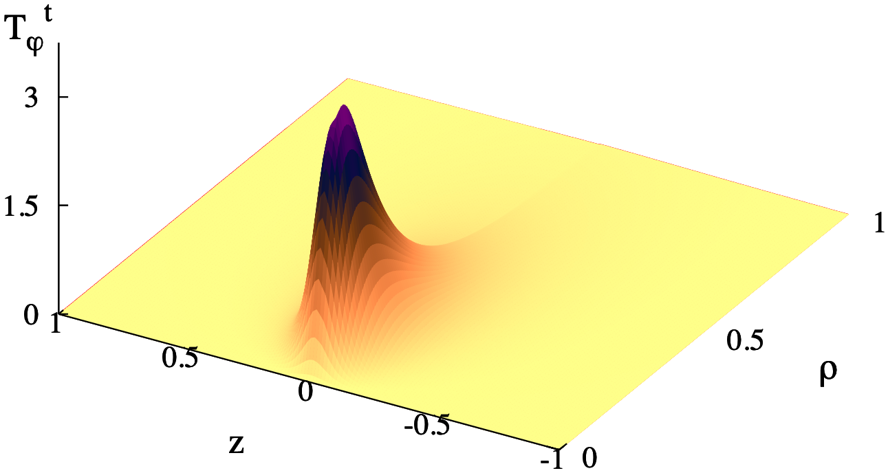
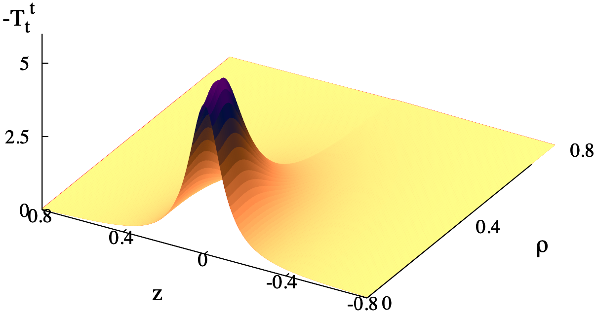
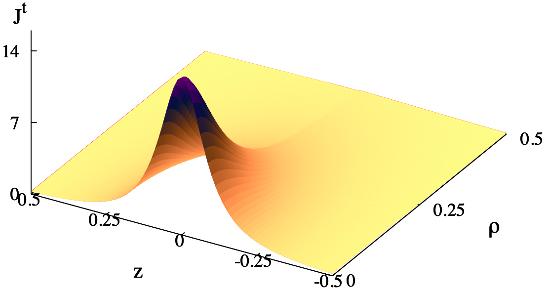
Figure 4: Same as Figure 3 for a spinning gauged Dirac stars with $m=1/2$ and the same values of $w,q$ and $\mu$.

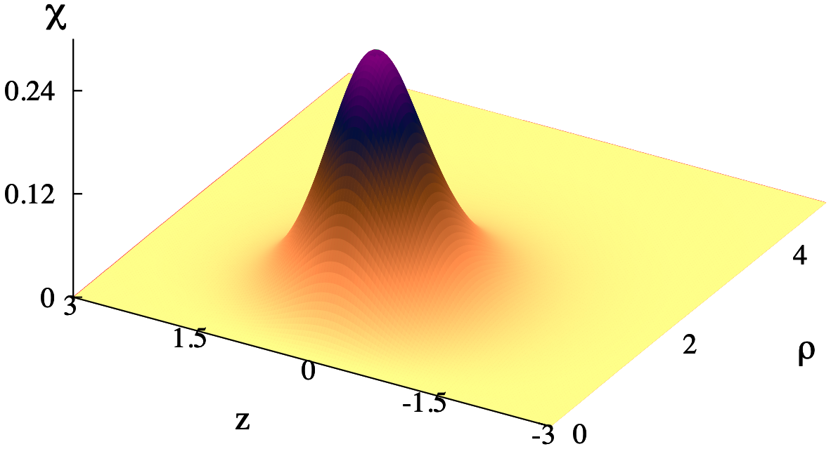
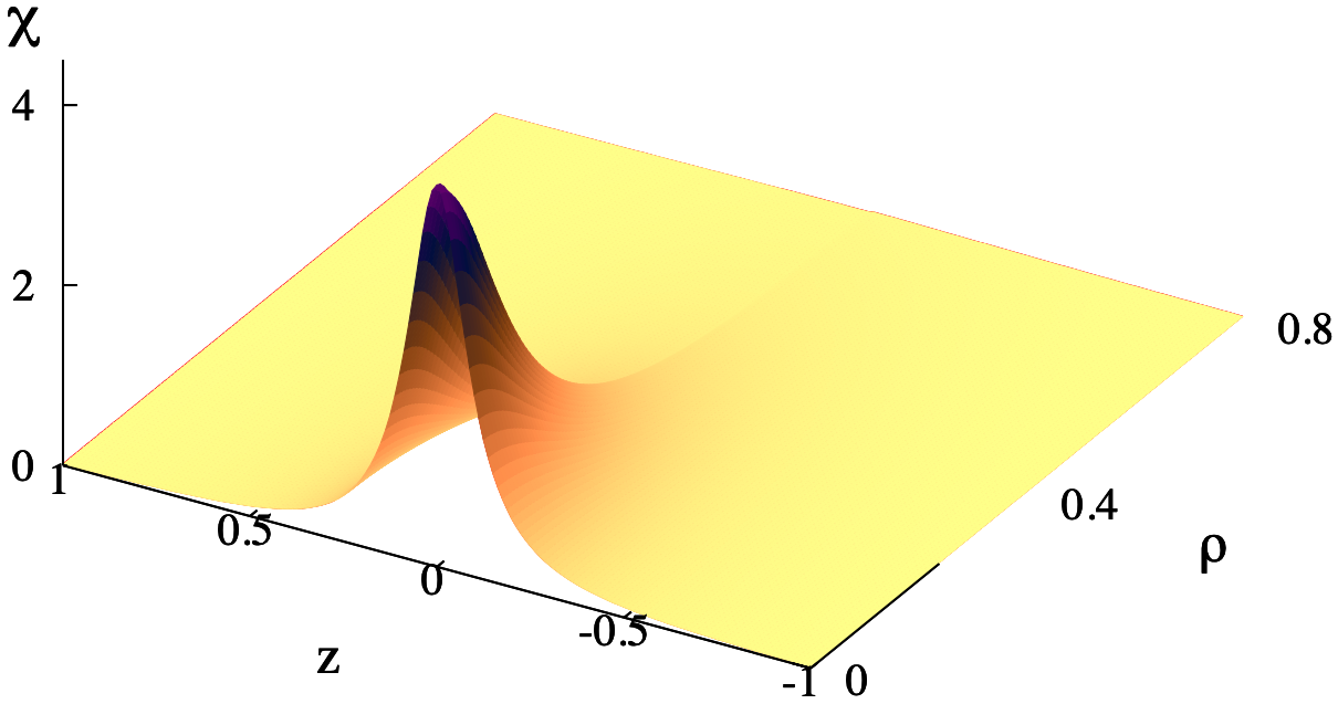
Figure 5: The quantity $\chi=\left(T_{\mu\nu}-\frac{1}{2}Tg_{\mu\nu}\right)X^{\mu}X^{\nu}$ (with the timelike vector $X^{\mu}$, $X^{\mu}X_{\mu}=-1$) is shown for the a spinning gauged boson (left panel) star and a Dirac (right panel) star, which correspond to the solutions in Figures 3 and 4. The strong energy condition $\chi\geq 0$ is satisfied in both cases.

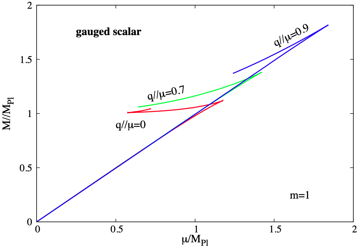
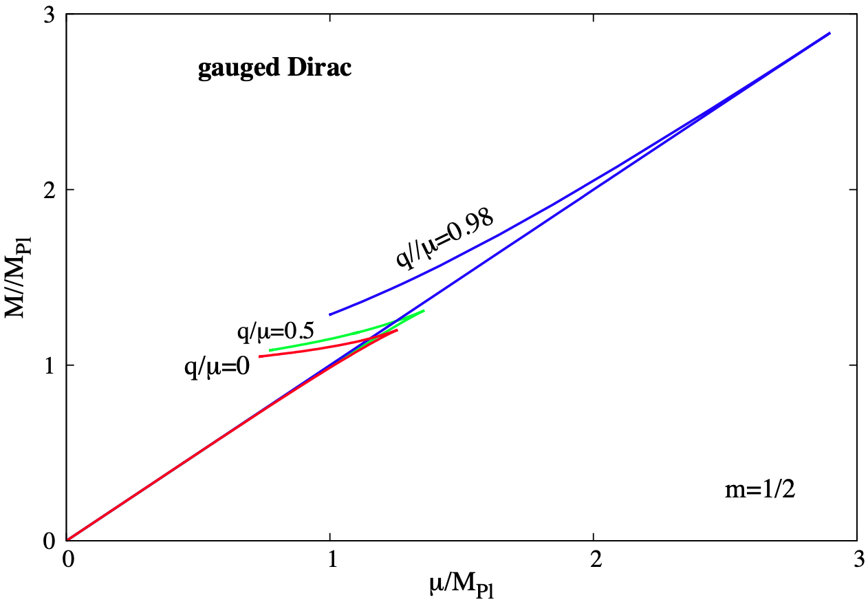
Figure 6: (Left panel) The mass $M$ $vs.$ scalar field mass $\mu$, in Planck units is shown for the three values of the invariant ratio $q/M$ (where $q$ is the gauge coupling constant). (Right panel) Same for the gauged Dirac case. In both cases, the single particle condition $Q=1$ is imposed.

3.3 The one particle picture

The results above are found for a classical treatment of the fields. In particular, the particle number is arbitrary and results from the numerical output for some given physical parameters $(w,\mu,q)$. If one tries to go beyond the classical field theory analysis and impose the quantum nature of fermions, this requires $Q=1$ for Dirac stars. This condition can also be imposed for boson stars, although in this case it is not a mandatory requirement.

As noticed in the original work [17], the one particle condition can be imposed by making use of a scaling symmetry of the equations. That is, given a numerical solution with $Q^{\rm(num)}$, one uses (3.30) with $\lambda=\sqrt{Q^{\rm(num)}}$, such that the scaled solution has $Q=1$ and $Q_{e}=q$. Then, as discussed in [1], the $(w,M)$-curves in Figures 1, 2. are not sequences of solutions with constant $\mu$, $q$ and varying $M$ (and $Q$); rather, it is a sequence with constant $Q=1$ and varying $\mu$ and $q$. Thus, since $\mu$, $q$ are parameters in the action, the curves would correspond to sequences of solutions of different models.

The resulting picture is shown in Figure 6, where we plot same of the data as in Figure 1 but imposing the single particle condition. One can see that the maximal mass for both the solutions’ mass and field mass is of order of the Planck mass.

4 Conclusions

The main purpose of this work was to provide a comparative analysis of two different types of solitonic solutions of GR-matter systems, with matter fields of spin $0$ and $1/2$, respectively. Here, and different from the previous study in [2], the scalar and Dirac fields are gauged, with a $local$ $U(1)$ symmetry.

We have confirmed that, as classical field theory solutions, gauging the fields still does not lead to a clear distinction between the fermionic/bosonic nature of the field, the configurations, which still possess a variety of similar features. Interestingly, the gyromagnetic ratio of the solutions appears as a distinguishing feature, with values around 1 for the scalar stars and 2 for the Dirac stars. It would be interesting to study also spinning gauged Proca stars and in particular consider their gyromagnetic ratio

Finally, let us remark on another difference between the models. The gauged spinning scalar boson stars can be in equilibrium with a black hole horizon [13]. This still does not seem to be possible for the Dirac case.

References

- [1] C. A. R. Herdeiro, A. M. Pombo and E. Radu, Phys. Lett. B 773 (2017) 654 [arXiv:1708.05674 [gr-qc]].
- [2] C. Herdeiro, I. Perapechka, E. Radu and Y. Shnir, Phys. Lett. B 797 (2019), 134845 [arXiv:1906.05386 [gr-qc]].
- [3] C. A. R. Herdeiro, A. M. Pombo, E. Radu, P. Cunha, V.P. and N. Sanchis-Gual, JCAP 04 (2021), 051 [arXiv:2102.01703 [gr-qc]].
- [4] J. C. Bustillo, N. Sanchis-Gual, A. Torres-Forné, J. A. Font, A. Vajpeyi, R. Smith, C. Herdeiro, E. Radu and S. H. W. Leong, Phys. Rev. Lett. 126 (2021) no.8, 081101 [arXiv:2009.05376 [gr-qc]].
- [5] D. J. Kaup, Phys. Rev. 172 (1968), 1331-1342
- [6] R. Ruffini and S. Bonazzola, Phys. Rev. 187 (1969), 1767-1783
- [7] P. Jetzer and J. J. van der Bij, Phys. Lett. B 227 (1989) 341.
- [8] D. Pugliese, H. Quevedo, J. A. Rueda H. and R. Ruffini, Phys. Rev. D 88 (2013) 024053 [arXiv:1305.4241 [astro-ph.HE]].
- [9] F. E. Schunck and E. W. Mielke, Phys. Lett. A 249 (1998) 389.
- [10] S. Yoshida and Y. Eriguchi, Phys. Rev. D 56 (1997) 762.
- [11] B. Kleihaus, J. Kunz and M. List, Phys. Rev. D 72 (2005) 064002 [arXiv:gr-qc/0505143].
- [12] B. Kleihaus, J. Kunz, M. List and I. Schaffer, Phys. Rev. D 77 (2008) 064025 [arXiv:0712.3742 [gr-qc]].
- [13] J. F. M. Delgado, C. A. R. Herdeiro, E. Radu and H. Runarsson, Phys. Lett. B 761 (2016), 234-241 [arXiv:1608.00631 [gr-qc]].
- [14] Y. Brihaye, T. Caebergs and T. Delsate, arXiv:0907.0913 [gr-qc].
- [15] L. G. Collodel, B. Kleihaus and J. Kunz, Phys. Rev. D 99 (2019) no.10, 104076 [arXiv:1901.11522 [gr-qc]].
- [16] B. Kleihaus, J. Kunz and F. Navarro-Lerida, Class. Quant. Grav. 33 (2016) no.23, 234002 [arXiv:1609.07357 [hep-th]].
- [17] F. Finster, J. Smoller and S. T. Yau, Phys. Rev. D 59 (1999), 104020 [arXiv:gr-qc/9801079 [gr-qc]].
- [18] F. Finster, J. Smoller and S. T. Yau, Phys. Lett. A 259 (1999), 431-436 [arXiv:gr-qc/9802012 [gr-qc]].
- [19] B. Carter, Phys. Rev. 174 (1968), 1559-1571
- [20] L. Morel, Z- Yao, P. Cladé et al. Nature 588 (2020) 61
- [21] D. Garfinkle and J. H. Traschen, Phys. Rev. D 42 (1990), 419-423
- [22] I. B. Khriplovich and A. A. Pomeransky, J. Exp. Theor. Phys. 86 (1998), 839-849
- [23] H. Pfister and M. King, Phys. Rev. D 65 (2002), 084033
- [24] H. Pfister and M. King, Class. Quant. Grav. 20 (2002), 205.
- [25] C. A. R. Herdeiro and E. Radu, Symmetry 12 (2020) no.12, 2032 [arXiv:2012.03595 [gr-qc]].
- [26] P. Jetzer, P. Liljenberg and B. S. Skagerstam, Astropart. Phys. 1 (1993) 429 [astro-ph/9305014].
- [27] S. R. Dolan and D. Dempsey, Class. Quant. Grav. 32 (2015) no.18, 184001 [arXiv:1504.03190 [gr-qc]].
- [28] D. R. Brill and J. A. Wheeler, Rev. Mod. Phys. 29 (1957) 465.
- [29] S. Dolan and J. Gair, Class. Quant. Grav. 26 (2009) 175020 [arXiv:0905.2974 [gr-qc]].
- [30] M. Soler, Phys. Rev. D 1 (1970) 2766.
- [31] R. Finkelstein, R. LeLevier and M. Ruderman, Phys. Rev. 83 (1951) 326.
-
[32]
W. Schönauer and R. Weiß,
J. Comput. Appl. Math. 27, 279 (1989) 279;
M. Schauder, R. Weiß and W. Schönauer, Universität Karlsruhe, Interner Bericht Nr. 46/92 (1992). -
[33]
N.I.M. Gould, J.A. Scott and Y. Hu,
ACM Transactions on Mathematical Software 33 (2007) 10;
O. Schenk and K. Gärtner Future Generation Computer Systems 20 (3) (2004) 475.