Decomposition of stellar populations in CosmoDC2 galaxies using SCARLET and Deep Learning

Abstract

We are presenting a novel, Deep Learning based approach to estimate the normalized broadband spectral energy distribution (SED) of different stellar populations in synthetic galaxies. In contrast to the non-parametric multiband source separation algorithm, SCARLET - where the SED and morphology are simultaneously fitted - in our study we provide a morphology-independent, statistical determination of the SEDs, where we only use the color distribution of the galaxy. We developed a neural network (sedNN) that accurately predicts the SEDs of the old, red and young, blue stellar populations of realistic synthetic galaxies from the color distribution of the galaxy-related pixels in simulated broadband images. We trained and tested the network on a subset of the recently published CosmoDC2 simulated galaxy catalog containing about 3,600 galaxies. The model performance was compared to the results of SCARLET, where we found that sedNN can predict the SEDs with 4-5% accuracy on average, which is about two times better than applying SCARLET. We also investigated the effect of this improvement on the flux determination accuracy of the bulge and disk. We found that using more accurate SEDs decreases the error in the flux determination of the components by approximately 30%.

1 Introduction

The proper mechanism of the galaxy evolution is an active research area where the analysis of the bulge-disk relation and stellar population properties are crucial. Spiral galaxies have significant bimodality in their stellar composition. The disk and the spiral arms are composed of a young, blue stellar population and the central region, the bulge contains mostly old, red stars. The proper separation of the two components in multiband photometric surveys can help to understand the stellar evolution inside spiral galaxies. It is often called as a blind source separation problem, since we do not know the exact broadband spectral energy distribution (SED) and the morphology of the sources. There are two main groups of source separation algorithms: parametric and non-parametric methods.
In case of parametric models we assume a specific surface brightness profile for the two main components of spiral galaxies. In most cases we suppose that the disk has an exponential profile, while the bulge can be described by a de Vaucouleurs model de Vaucouleurs (1948). An alternative choice is the Sersic model, in which both components can be described but with different Sersic exponents ($n=1$ for the disk, and $n=4$ for the bulge). The assumed model is then fitted to the galaxy image measured in single-band or multiband surveys. Such source separation algorithms are for example PSFex Bertin (2011) or Megamorph Vika et al. (2013) fitting codes. The obvious disadvantage of this approach is that complex structures of galaxies cannot be reproduced, and we strongly rely on assumptions regarding the brightness distribution of the galaxy.
The other way of separating different sources from each other is to exploit the diversity of their SEDs. Let’s assume that we have $N_{s}=2$ sources, namely the bulge and the disk. We know that they are composed of different stellar populations, hence they are characterized by two different SEDs. This means that if we have images at $N_{b}\geq N_{s}$ distinct broadband filters, then the intensity distribution of the sources can be estimated by solving a linear system of equations. Let us denote the data observed in $N_{b}$ filters as $[y_{i}]_{i=1,...,N_{b}}$. It is then a linear combination of $N_{s}$ sources, see Equation 1.

$$y_{i}[k]=\sum\limits_{j=1}^{N_{s}}a_{i,j}x_{j}[k]+z_{i}[k],$$ (1)

where $y_{i}[k]$ is the $k$th pixel of the original image in the $i$th band, $a_{i,j}$ and $x_{j}[k]$ contain the SEDs and the morphology of the sources, respectively and $z_{i}[k]$ is a noise term. Let’s rewrite this in matrix form, see Equation 2

$$Y=AX+Z,$$ (2)

where $Y$ and $Z$ are $N_{b}\times N_{p}$ matrices ($N_{p}$ is the number of pixels), $A$ is the SED mixing matrix and $X$ is the $N_{s}\times N_{p}$ matrix, which contains the components $x_{j}$. The MuSCADeT algorithm Joseph, R. et al. (2016) is designed to deblend different astronomical sources having different SEDs. Its performance was demonstrated mainly in the separation of blended objects due to strong gravitational lensing, but it is also able to disentangle a single galaxy, as was shown on a spiral galaxy with significantly high colour-contrast in the original paper Joseph, R. et al. (2016). It is a multi-channel extension of the morphological component analysis (MCA) described in Starck et al. (2004). To the best of our knowledge our work is the first in applying non-parametric source separation algorithm on a large number of synthetic galaxies to get the bulge and disk components.
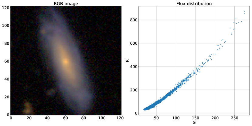
The main challenge of this approach is that we neither know the SEDs nor the morphology of the galaxy components. There are two ways to address this problem: 1) one is to first estimate somehow the SEDs and then fix them during the morphology fitting, or 2) fit both of them and introduce some constraints to reduce degeneracy (e.g. positivity, monotonicity, symmetry constraints). MuSCADeT belongs to the first group, where the $A$ mixing matrix can be a user defined parameter, but an automated SED analysing process based on principal component analysis (PCA) is also available. This pre-processing method essentially searches for bright regions and performs PCA in the $N_{b}$ dimensional space spanned by the broadband filters. Hence, the pixels having proportional SEDs - meaning that they belong to the same stellar population - will be distributed along the first few PCA axes, and one can identify them using some clustering algorithm and get the mean of their SEDs. This method can be powerful, if the different stellar populations are similarly bright, both causing significant signal in the principal component analysis. The problem is that in most of the spiral galaxies there is a very bright red bulge, and some faint blue spiral arms, see Figure 1. In the flux distribution plot we can see that there is a very large brightness gradient, and a slight curvature of the distribution can be also observed. This curvature is due to the simultaneously changing in brightness and color from blue to red. As we can see there is no clear difference between the two stellar populations in the filter space. Therefore we had to use a different approach to determine the spectral energy distributions of the red and blue regions. Another drawback of MuSCADeT is that it does not take the PSF convolution into account during deblending.
A more sophisticated framework is SCARLET Melchior et al. (2018), which is based on a generalization of non-negative matrix factorization to alternative and several simultaneous constraints. It can simultaneously fit the SEDs and the morphology, and it also applies the PSF convolution. The main focus of this method is again to disentangle different galaxies from each other, since the upcoming sky surveys (e.g. LSST Ivezić et al. (2019)) will provide images of crowded regions in the far Universe. Therefore its performance was tested on separating synthetic overlapping galaxies from each other. Hence, besides the introduction and application of our novel approach we also provide a reliable test of SCARLET on separating synthetic galaxies into the bulge and disk components to which we have compared our results.
Separating stellar populations inside a galaxy can be much more difficult, since the flux contribution of them is often very different (e.g. irregular galaxies with small bulge and bright star-forming regions, or older, more evolved spiral galaxies with a massive bulge and faint blue spiral arms). Moreover, in most of the cases the two stellar populations are strongly overlapping and there is no region of the galaxy where only one of the components has a flux contribution. This fact causes high degeneracy in the SED-morphology determination and therefore there is a strong need for a morphology-independent estimation of the SEDs. In our study we have investigated simulated galaxies with different flux contributions of the bulge and disk components, and estimated their SEDs. We trained a neural network (sedNN) in the Keras framework that can predict the two SEDs directly from the color distribution of the galaxy. The resulting SEDs were used as input in the morphology determination of the two sources in a TensorFlow model. This paper is organized as follows: in Section 2 we introduce the synthetic data we used, in Section 3 we explain the pre-processing steps for creating the best input data as well as the architecture of our neural network, in Section 4 we show our results made on the data as well as the comparison to SCARLET and finally in Section 5 we discuss and summarize the key findings of our work.

Figure 1: An example galaxy (RA: 41.422048, DEC: -9.074144) from the Dark Energy Survey (DES). Left: RGB image of the galaxy using the $G$, $R$, $I$ filters based on the algorithm of Lupton et al. (2004). Right: Distribution of pixels in the $G-R$ flux space.

2 Data

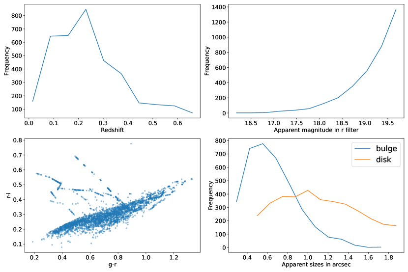
We used the recently published data of CosmoDC2 synthetic sky catalog Korytov et al. (2019), which is designed to support precision dark energy science with LSST. The catalog is based on a trillion-particle, $(4.225Gpc)^{3}$ box cosmological N-body simulation. Among many properties each galaxy is characterized by a unique morphology, spectral energy distributions and broadband filter magnitudes. This catalog was constructed using empirical methods with a semi-analyitic modeling using the Galacticus code Benson (2012). The simulated galaxies are composed of a bulge and disk both having a Sersic profile with $n=4$ and $n=1$, respectively. Galacticus follows the evolution of the components separately. The bulge is formed as a result of galaxy mergers or via instabilities of the galactic disk. Hence, we could use unbiased data of highly realistic galaxy components, where all necessary parameters were given, such as apparent magnitudes in the LSST g, r, i, z filters, shear parameters and brightness profile to describe the morphology as well as the redshifts. To get a convenient subset of galaxies we made some filtering in three parameters using 5 tiles of CosmoDC2 (8786, 8787, 8788, 8789 and 8790): 1) we searched for relatively bright galaxies with an apparent magnitude of LSST r band of $m_{r}<20.0$; 2) we made a cut in the half light right radius ($r_{hl}$) of the disk component: $0.5\geq r_{hl}\geq 2.0$ arcsec to avoid unresolvable galaxy components as well as hanging over from the image and 3) obviously we required exactly 2-component galaxies by setting the bulge-to-total flux ratio ($BT$) between $0.1\geq BT\geq 0.9$. After some preliminary investigation of the filtered data we found that a huge amount of the galaxies have components with almost the same SED. Therefore we calculated the angle ($\alpha$) between the four-element SED vectors of the bulge and disk and we made a final filtering for galaxies where $\alpha>0.1$ radian. Hence the remaining dataset consisted about 3,600 synthetic galaxies. This dataset was splitted into training, validation and test set with sizes of 2369, 539 and 704, respectively. The distributions of the most important properties of the galaxies can be seen in Figure 2.
To generate simulated LSST images of the galaxies we used the popular GalSim code Rowe et al. (2015). We have calibrated the pixel intensities ($I$) to the apparent magnitude ($m$) according to equation 3 similar to the Dark Energy Survey (DES) Abbott et al. (2021).

$$m=30-2.5\log_{10}I$$ (3)

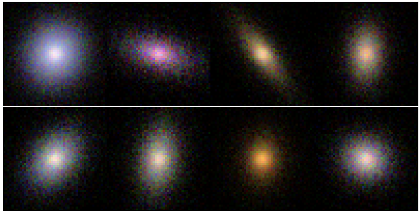
The pixel resolution was set to 0.2 arcsec and the brightness distributions have been convolved with a Gaussian PSF having a FWHM of 0.7 arcsec in all filters. Finally, we added a simple Poisson noise on the 50x50x4 images to get more realistic measurements. In Figure 3 we plotted some of the synthetic galaxies for illustration purposes.

Figure 2: Distributions of important galaxy properties. Top row: Redshift and apparent $r$ filter magnitude distribution of the galaxies. Bottom row: $g-r$ and $r-i$ color index distribution of the galaxies as well as the apparent size distribution (half-light radius) of the bulge and disk measured in arcsec.

Figure 3: Randomly selected galaxies from our synthetic dataset.

3 Methods

3.1 Pre-processing of the data

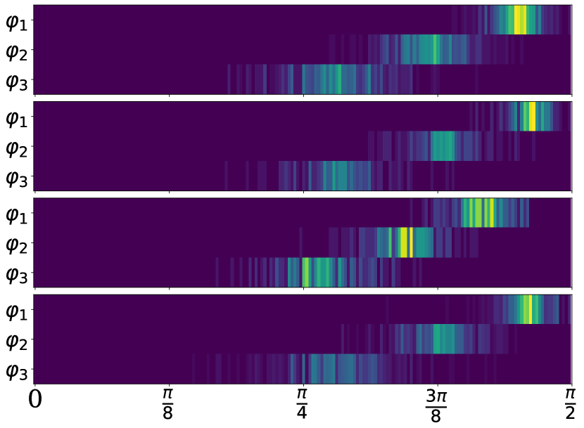
In order to provide the most relevant data for the SED predicting neural network (sedNN) we extracted the color distribution of the galaxy inside a predefined mask. In this context color means the directional angle of the pixel vectors in the 4 dimensional magnitude space. Since the pixel values of the sources should be positive, their angle coordinates will be in the range of $\varphi_{1},\varphi_{2},\varphi_{3}\in[0,\pi/2]$. We divided this range into 180 bins, hence we ended up with 3x180 matrices (see Figure 4), which were later flattened for the neural network. It is worth mentioning that these matrices are independent from the exact morphology, they only show the statistics of the pixel colors.
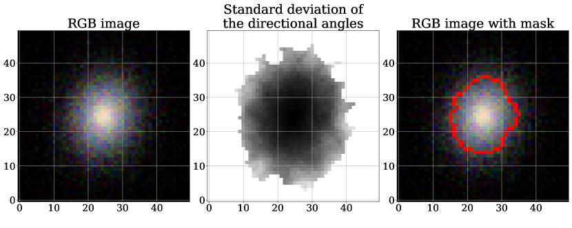
For the mask determination we calculated first a color noise map, where the standard deviation of colors were calculated inside a 5x5 sliding window (see Figure 5). We made a cut in the color noise map at 0.2 radian above which mostly the noisy edge of the galaxy can be found and which would debase the quality of the color histograms.

Figure 4: Color distribution in the 3 angle coordinates of four randomly selected galaxies. Colors indicates the number density in the bins.

Figure 5: Mask determination using the color noise map.

3.2 Network architecture of sedNN

First we started with a network architecture of three fully connected hidden and dropout layers, one input and one output layer. All layers use elu activation function to avoid vanishing gradients. For training we used ADAM optimizer with a learning rate of 0.001, mean squared error loss function and a batch size of 128. To find the best performing structure we applied a grid search over two important hyperparameters, namely the dropout rate and the number of neurons in each hidden layer. We found that using a grid of number of neuronsxdropout rate=[80,100,120,140]x[0.1,0.2,0.3,0.4,0.5] the best performing network has 120 neurons and a dropout rate of 0.2. We summarized these properties in Table 1.
In the output layer we restricted the network to give such SEDs, which sum up exactly to one. This criterion was achieved by predicting only the first 3 components of the SED vectors (hence, the output dimension was 2x3=6) and calculating the last one by subtracting them from one. The network was then trained on these 8-element vectors containing the SEDs of the bulge and disk components.

Table 1: Hyperparameters of sedNN defining its architecture and the training process.

Parameter	Value
Number of hidden layers	3
Number of neurons per layer	120
Dropout rate	0.2
Activation function	elu
Optimizer	Adam
Loss function	Mean Squared Error
Batch size	128
Initial learning rate	0.001

4 Results

4.1 Predicting the SEDs

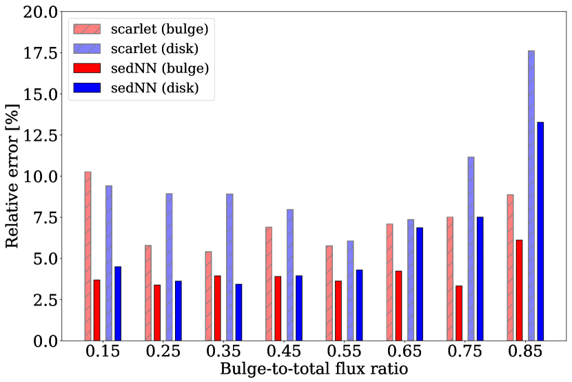
We evaluated the sedNN model performance on the test set grouped by the bulge-to-total flux ratios in 0.1 wide bins. For comparison we applied SCARLET on this subset as well, where we found that at all bulge-to-total flux ratios sedNN provided more accurate results (see Figure 6). We used the MultiExtendedSource class of SCARLET, where we gave the center of the object and the original PSF, and we set the number of components to $K=2$. In the simultaneous fitting process of the SEDs and morphology we used a maximum of 600 iteration and e_rel$=10^{-6}$.
We calculated the relative root mean squared error according to $RelRMS=RMS(SED_{original},SED_{predicted})/SED_{original}$. We can see that on average the prediction efficiency of sedNN is between 3.3-6.1% and 3.4-13.2% for the bulge and disk, respectively. Contrarily, in case of SCARLET these errors are between 5.4-10.2% and 6.1-17.6%, which is about two times worse than sedNN. It is remarkable that in case of only 0.1 flux contribution of the bulge sedNN is able to predict its SED with 3.7% as against to SCARLET 10.3% efficiency. This indicates that one can more effectively predict the SEDs using the color distribution of the pixels than solving the whole source separation problem. The SED estimation performance of the disk is however worse in case of its low flux contribution (at $BT\approx 0.9$), which is mainly due to the low signal-to-noise ration near the edge of the galaxy. Nevertheless, even in this case sedNN prediction is 5% better than using SCARLET.

Figure 6: Relative error in the SED determination. Results are compared with SCARLET.

4.2 Deblending the galaxies

Since we have compared our results to SCARLET, in this study we also tested the deblending performance of SCARLET on the morphology determination of the bulge and disk. In the following we present the correlation between the derived and original components according to the same equation used in Melchior et al. (2018) (see Eq. 4) as well as the relative flux error of the components.

$$\zeta_{\nu}=\frac{\nu_{true}\nu_{observed}}{\sqrt{\nu_{true}\nu_{true}}\sqrt{\nu_{observed}\nu_{observed}}}$$ (4)

We calculated these measures for the original deblending – where the SED and the morphology are simultaneously fitted – and we also repeated the source separation process while fixing the SEDs of the components to the more accurate values predicted by sedNN. In SCARLET by default the total flux of the components in each band is fitted through the SEDs and the morphology matrices are restricted with a normalization constraint. Since we only provide the normalized SED we had to make some modifications to fit the total fluxes through the morphology. In the following we have compared the PSF convolved brightness distributions to avoid potential systematic effects of the deconvolved images.

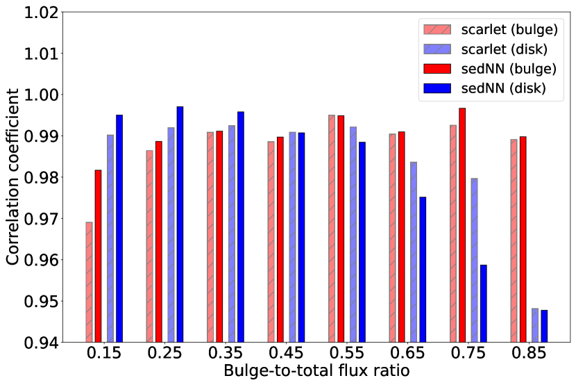
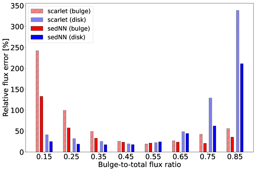
In Figure 7 we plotted the correlation coefficients at the different bulge-to-total flux ratios. We can observe that the better SEDs improve the morphology determination mostly below $BT<0.5$ and near to the two edges of the bulge-to-flux ratios. In Figure 8 we plotted the relative error in the flux determination of the components. The improvement is now more significant where the relative error is about 30% smaller if we provide the more accurate SEDs and fix them during the source separation process. These results clearly shows us that SCARLET performs well in the simultaneous fitting if the two components are equally bright. However, in situations where the bulge is less dominant (e.g. in irregular galaxies) or the disk is very faint (e.g. old spiral galaxies with a large bulge) the improvement of the SED prediction results in a significant improvement in the flux estimation as well.

Figure 7: Correlation between the derived and the true morphologies of the galaxy components.

Figure 8: Relative error in the flux determination of the components.

5 Conclusions

In our work we developed a morphology-independent method to estimate the normalized broadband spectral energy distributions of the two main stellar populations in simulated disk galaxies, where we exploit the relation between the observable color distribution of the pixels and the real SEDs. We built a neural network (sedNN) which has been successfully trained on realistic simulated galaxies of CosmoDC2 to predict the real SEDs of the blue and red stellar population even if the flux contribution of them is very different. These accurate estimations were further given to SCARLET. We have shown that in the case of the used simulated galaxies our two-step approach has in most cases better deblending performance than simultaneously fitting the SEDs and the morphology with Scarlet, although the reproduction error of the components is still high. This shows us how difficult is the model-independent bulge-disk separation of spiral galaxies even in case of a synthetic galaxy catalog.
The developed model could be applied for real observations of spiral galaxies where we could use Integral Field Spectroscopy measurements to create the ground truth values for the broadband spectral energy distributions.

Data Availability

We used data from the public archives of CosmoDC2 galaxy catalog. The further processed data as well as the model architecture of sedNN are also available at https://github.com/skunsagimate/sedNN.

References

- Abbott et al. (2021) Abbott T. M. C., et al., 2021, ApJS, 255, 20
- Benson (2012) Benson A. J., 2012, New Astron., 17, 175
- Bertin (2011) Bertin E., 2011, in Evans I. N., Accomazzi A., Mink D. J., Rots A. H., eds, Astronomical Society of the Pacific Conference Series Vol. 442, Astronomical Data Analysis Software and Systems XX. p. 435
- Ivezić et al. (2019) Ivezić Ž., et al., 2019, ApJ, 873, 111
- Joseph, R. et al. (2016) Joseph, R. Courbin, F. Starck, J.-L. 2016, A&A, 589, A2
- Korytov et al. (2019) Korytov D., et al., 2019, ApJS, 245, 26
- Lupton et al. (2004) Lupton R., Blanton M. R., Fekete G., Hogg D. W., O’Mullane W., Szalay A., Wherry N., 2004, Publications of the Astronomical Society of the Pacific, 116, 133–137
- Melchior et al. (2018) Melchior P., Moolekamp F., Jerdee M., Armstrong R., Sun A. L., Bosch J., Lupton R., 2018, Astronomy and Computing, 24, 129
- Rowe et al. (2015) Rowe B. T. P., et al., 2015, Astronomy and Computing, 10, 121
- Starck et al. (2004) Starck J.-L., Elad M., Donoho D., 2004, Advances in Imaging and Electron Physics - ADV IMAG ELECTRON PHYS, 132, 287
- Vika et al. (2013) Vika M., Bamford S. P., Häußler B., Rojas A. L., Borch A., Nichol R. C., 2013, Monthly Notices of the Royal Astronomical Society, 435, 623
- de Vaucouleurs (1948) de Vaucouleurs G., 1948, Annales d’Astrophysique, 11, 247