Broad Ranges of Investment Configurations for Renewable Power Systems, Robust to Cost Uncertainty and Near-Optimality

Abstract

To achieve ambitious greenhouse gas emission reduction targets in time, the planning of future energy systems needs to accommodate societal preferences, e.g. low levels of acceptance for transmission expansion or onshore wind turbines, and must also acknowledge the inherent uncertainties of technology cost projections. To date, however, many capacity expansion models lean heavily towards only minimising system cost and only studying few cost projections. Here, we address both criticisms in unison. While taking account of technology cost uncertainties, we apply methods from multi-objective optimisation to explore trade-offs in a fully renewable European electricity system between increasing system cost and extremising the use of individual technologies for generating, storing and transmitting electricity to build robust insights about what actions are viable within given cost ranges. We identify boundary conditions that must be met for cost-efficiency regardless of how cost developments will unfold; for instance, that some grid reinforcement and long-term storage alongside a significant amount of wind capacity appear essential. But, foremost, we reveal that near the cost-optimum a broad spectrum of regionally and technologically diverse options exists in any case, which allows policymakers to navigate around public acceptance issues. The analysis requires to manage many computationally demanding scenario runs efficiently, for which we leverage multi-fidelity surrogate modelling techniques using sparse polynomial chaos expansions and low-discrepancy sampling.

1 Introduction

Energy system models have become a pivotal instrument for policy-making to find cost-efficient system layouts that satisfy ambitious climate change mitigation targets. But even though they have proliferated in spatial, temporal, technological and sectoral detail and scope in recent years, least-cost optimisation models can easily give a false sense of exactness [1, 2]. Frequently, they present just a single least-cost solution for a single set of cost assumptions, which not only neglects uncertainties inherent to technology cost projections which capacity expansion models are susceptible to [3, 4, 5], but also hides a wide array of alternative solutions that are equally feasible and only marginally more expensive [6, 7, 8].

Trade-offs revealed by deviating from least-cost solutions are extremely attractive for policymakers, because they allow them to make decisions based on non-economic criteria without affecting the cost-effectiveness of the system. Knowing that many similarly costly but technologically diverse solutions exist, helps to accommodate political and social dimensions that are otherwise hard to quantify; for instance, rising public opposition towards reinforced transmission lines and onshore wind turbines or an uneven distribution of new infrastructure [9, 8, 10].

Techniques like multi-objective optimisation and modelling-to-generate-alternatives are designed to find such near-optimal solutions. Among others, they have been applied to investment planning models of the European [6], the Italian [7], and the United States power system [11], pathways to decarbonise the power system of the United Kingdom [12], a single-node sector-coupling model of Germany [13], global integrated assessment models [14], and were combined with a quick hull algorithm to span a polytope of low-cost solutions for a single set of cost parameters [15].

However, most of the studies above only use a central cost projection for each considered technology. But recent decades have shown that many of these projections contain a high level of uncertainty, particularly for fast-moving technologies like solar, batteries and hydrogen storage. This uncertainty propagates through the model to strongly affect the optimal and near-optimal system compositions, thus undermining any analysis of the trade-offs. Hence, it is crucial that apparent compromises are rigorously tested for robustness to technology cost uncertainty to raise confidence in conclusions about viable, cost-effective power system designs. To thoroughly sweep the uncertainty space, we can fortunately avail of previous works on multi-dimensional global sensitivity analysis techniques in the context of least-cost optimisation [3, 16, 17, 18, 19]. We expand their application to strengthening insights on the scope of near-optimal trade-offs, wherein the novelty of this contribution lies.

Here, we systematically explore robust trade-offs near the cost-optimum of a fully renewable European electricity system model, and investigate how they are affected by uncertain technology cost projections. Thereby, we evaluate both compromises between system cost and technology choices, as well as between pairs of technologies. We do so by solving numerous spatially and temporally explicit long-term investment planning problems that coordinate generation, transmission and storage investments subject to multi-period linear optimal power flow constraints, while employing methods from global sensitivity analysis to account for a wide range of cost projections for wind, solar, battery and hydrogen storage technologies.

To handle the immense computational burden incurred by searching for near-optimal alternatives alongside evaluating many different cost parameter sets, we employ multi-fidelity surrogate modelling techniques, based on sparse polynomial chaos expansion that allow us to merge results from one simpler and another more detailed model. This approach has been proven very effective in Tröndle et al. [3]. Heavy parallelisation with high-performance computing infrastructure allowed us to solve more than 50,000 resource-intensive optimisation problems which, in combination with surrogate modelling, admit spanning a probabilistic space of near-optimal solutions rather than putting single scenarios into the foreground.

Thereby, we are able to present alternative solutions beyond least-cost that have a high chance of involving a limited cost increase, just as we identify regions that are unlikely to be cost-efficient. We derive both ranges of options and technology-specific boundary conditions, that are not affected by cost uncertainty and must be met to keep the total system cost within a specified range. Our results show that indeed many such similarly costly but technologically diverse solutions exist regardless of how technology cost developments will unfold within the considered ranges.

2 Methods

In this section, we first outline how we obtain least-cost and near-optimal solutions for a given cost parameter set. We then describe the model of the European power system and define the cost uncertainties. Finally, we explain how we make use of multi-fidelity surrogate modelling techniques based on polynomial chaos expansions and find an experimental design that efficiently covers the parameter space.

2.1 Least-Cost Investment Planning

The objective of long-term power system planning is to minimise the total annual system costs, comprising annualised capital costs $c_{\star}$ for investments at locations $i$ in generator capacity $G_{i,r}$ of technology $r$, storage capacity $H_{i,s}$ of technology $s$, and transmission line capacities $F_{\ell}$, as well as the variable operating costs $o_{\star}$ for generator dispatch $g_{i,r,t}$:

$$\min_{G,H,F,g}\quad\left\{\sum_{i,r}c_{i,r}\cdot G_{i,r}+\sum_{i,s}c_{i,s}\cdot H_{i,s}+\sum_{\ell}c_{\ell}\cdot F_{\ell}+\sum_{i,r,t}w_{t}\cdot o_{i,r}\cdot g_{i,r,t}\right\}$$ (1)

where the snapshots $t$ are weighted by $w_{t}$ such that their total duration adds up to one year. The objective is subject to a set of linear constraints that define limits on (i) the capacities of infrastructure from geographical and technical potentials, (ii) the availability of variable renewable energy sources for each location and point in time, and (iii) linearised multi-period optimal power flow (LOPF) constraints including storage consistency equations, which we describe in more detail in the following.

The capacities of generation, storage and transmission infrastructure are limited to their geographical potentials from above and existing infrastructure from below:

$$\underline{G}_{i,r}\leq G_{i,r}\leq\overline{G}_{i,r} \qquad\forall i,r$$ (2)

$$\underline{H}_{i,s}\leq H_{i,s}\leq\overline{H}_{i,s} \qquad\forall i,s$$ (3)

$$\underline{F}_{\ell}\leq F_{\ell}\leq\overline{F}_{\ell} \qquad\forall\ell$$ (4)

The dispatch of a renewable generator is constrained by its rated capacity and the time- and location-dependent availability $\overline{g}_{i,r,t}$, given in per-unit of the generator’s capacity:

$$0\leq g_{i,r,t}\leq\overline{g}_{i,r,t}G_{i,r}\qquad\forall i,r,t$$ (5)

The dispatch of storage units is described by a charge variable $h_{i,s,t}^{+}$ and a discharge variable $h_{i,s,t}^{-}$, each limited by the power rating $H_{i,s}$.

$$0\leq h_{i,s,t}^{+}\leq H_{i,s} \qquad\forall i,s,t$$ (6)

$$0\leq h_{i,s,t}^{-}\leq H_{i,s} \qquad\forall i,s,t$$ (7)

The energy levels $e_{i,s,t}$ of all storage units are linked to the dispatch by

$$e_{i,s,t}=\> \eta_{i,s,0}^{w_{t}}\cdot e_{i,s,t-1}+w_{t}\cdot h_{i,s,t}^{\text{inflow}}-w_{t}\cdot h_{i,s,t}^{\text{spillage}} \quad\forall i,s,t$$

$$+\eta_{i,s,+}\cdot w_{t}\cdot h_{i,s,t}^{+}-\eta_{i,s,-}^{-1}\cdot w_{t}\cdot h_{i,s,t}^{-}.$$ (8)

Storage units can have a standing loss $\eta_{i,s,0}$, a charging efficiency $\eta_{i,s,+}$, a discharging efficiency $\eta_{i,s,-}$, natural inflow $h_{i,s,t}^{\text{inflow}}$ and spillage $h_{i,s,t}^{\text{spillage}}$. The storage energy levels are assumed to be cyclic and are constrained by their energy capacity

$$e_{i,s,0}=e_{i,s,T} \qquad\forall i,s$$ (9)

$$0\leq e_{i,s,t}\leq\overline{T}_{s}\cdot H_{i,s} \qquad\forall i,s,t.$$ (10)

To reduce the number of decisison variables, we link the energy capacity to power ratings with a technology-specific parameter $\overline{T}_{s}$ that describes the maximum duration a storage unit can discharge at full power rating.

Kirchhoff’s Current Law (KCL) requires local generators and storage units as well as incoming or outgoing flows $f_{\ell,t}$ of incident transmission lines $\ell$ to balance the inelastic electricity demand $d_{i,t}$ at each location $i$ and snapshot $t$

$$\sum_{r}g_{i,r,t}+\sum_{s}h_{i,s,t}+\sum_{\ell}K_{i\ell}f_{\ell,t}=d_{i,t}\qquad\forall i,t,$$ (11)

where $K_{i\ell}$ is the incidence matrix of the network.

Kichhoff’s Voltage Law (KVL) imposes further constraints on the flow of AC lines. Using linearised load flow assumptions, the voltage angle difference around every closed cycle in the network must add up to zero. We formulate this constraint using a cycle basis $C_{\ell c}$ of the network graph where the independent cycles $c$ are expressed as directed linear combinations of lines $\ell$ [20]. This leads to the constraints

$$\sum_{\ell}C_{\ell c}\cdot x_{\ell}\cdot f_{\ell,t}=0\qquad\forall c,t$$ (12)

where $x_{\ell}$ is the series inductive reactance of line $\ell$. Controllable HVDC links are not affected by this constraint.

Finally, all line flows $f_{\ell,t}$ must be operated within their nominal capacities $F_{\ell}$

$$\left|f_{\ell,t}\right|\leq\overline{f}_{\ell}F_{\ell} \qquad\forall\ell,t,$$ (13)

where $\overline{f}_{\ell}$ acts as a per-unit buffer capacity to protect against the outage of single circuits.

This problem is implemented in the open-source tool PyPSA [21] and is solved by Gurobi. Note, that it assumes perfect foresight for a single reference year based on which capacities are optimised. It does not include pathway optimisation, nor aspects of reserve power, or system stability. Changes of line expansion to line impedance are ignored.

2.2 Near-Optimal Alternatives

Using the least-cost solution as an anchor, we use the $\epsilon$-constraint method from multi-objective optimisation to find near-optimal feasible solutions [6, 22]. For notational brevity, let $c^{\top}x$ denote the linear objective function Equation 1 and $Ax\leq b$ the set of linear constraints Equations 2 to 13 in a space of continuous variables, such that the minimised system cost can be represented by

$$C=\min_{x}\left\{c^{\top}x\mid Ax\leq b\right\}.$$ (14)

We then encode the original objective as a constraint such that the cost increase is limited to a given $\epsilon$. In other words, the feasible space is cut to solutions that are at most $\epsilon$ more expensive than the least-cost solution. Given this slack, we can formulate alternative search directions in the objective. For instance, we can seek to minimise the sum of solar installations $x_{s}\subseteq x$ with

$$\overline{x_{s}}=\min_{x_{s}}\left\{\>1^{\top}x_{s}\mid Ax\leq b,\quad c^{\top}x\leq(1+\epsilon)\cdot C\>\right\}.$$ (15)

To draw a full picture of the boundaries of the near-optimal feasible space, we systematically explore the extremes of various technologies: we both minimise and maximise the system-wide investments in solar, onshore wind, offshore wind, any wind, hydrogen storage, and battery storage capacities, as well as the total volume of transmission network expansion. Evaluating each of these technology groups for different cost deviations $\epsilon\in\{1\%,2\%,4\%,6\%,8\%\}$ allows us to observe how the degree of freedom regarding investment decisions rises as the optimality tolerance is increased, both at lower and upper ends. The boundaries delineate Pareto frontiers on which no criterion, neither reducing system cost nor extremising the capacity of a technology, can be improved without depressing the other. By arguments of convexity, these extremes even define limits within which all near-optimal solutions are contained. Moreover, although this scheme primarily studies aggregated capacities, the solutions are spatially explicit, and we can inspect for each case how the capacities of each technology are distributed within the network.

The near-optimal analysis above only explores the extremes of one technology at a time, i.e. one direction in the feasible space. But actually the space of attainable solutions within $\epsilon$ of the cost-optimum is multi-dimensional. To further investigate trade-offs between multiple technologies, in addition to the $\epsilon$-constraint and the objective to extremise capacities of a particular technology, we formulate a constraint that fixes the capacity of another technology. For instance, we search for the minimum amount of wind capacity $x_{w}\subseteq x$ given that a certain amount of solar is built

$$\overline{x_{w}}=\min_{x_{w}}\left\{\>1^{\top}x_{w}\mid Ax\leq b,\quad c^{\top}x\leq(1+\epsilon)\cdot C,\quad 1^{\top}x_{s}=\underline{x_{s}}+\alpha\cdot(\overline{x_{s}}-\underline{x_{s}})\>\right\}.$$ (16)

The $\alpha$ denotes the relative position within the near-optimal range of solar capacities at given $\epsilon$. For example, at $\alpha=0\%$ we look for the least wind capacity given that minimal solar capacities are built. An alternative but more complex approach to spanning the space of near-optimal solutions in multiple dimensions at a time using a quick hull algorithm was presented by Pedersen et al. [15].

Due to computational constraints, we focus on technologies which are assumed to lend themselves to substitution and limit the corresponding analysis to a single cost increase level of $\epsilon=6\%$. We consider the three pairs, (i) wind and solar, (ii) offshore and onshore wind, (iii) hydrogen and battery storage, by minimising and maximising the former while fixing the latter at positions $\alpha\in\{0\%,25\%,50\%,75\%,100\%\}$ within the respective near-optimal range.

2.3 Model Inputs

(a) low-fidelity:	(b) high-fidelity:
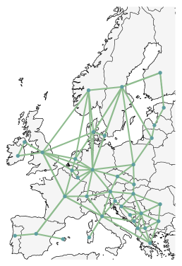
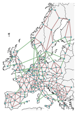
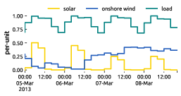
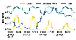
37 nodes and 4-hourly	128 nodes and 2-hourly

Figure 1: Spatial and temporal resolution of the low and high fidelity model. Green lines represent controllable HVDC lines. Red lines represent HVAC lines. The exemplary capacity factors for wind and solar are shown for four days in March at the northernmost node in Germany, alongside the normalised load profile.

The instances of the coordinated capacity expansion problem (Section 2.1) are based on PyPSA-Eur, which is an open model of the European power transmission system that combines high spatial and temporal resolution [23]. Because it only uses open data and every processing step is defined in a workflow [24], we achieve a high level of transparency and reproducibility. In the following, we outline the main features and configurations, and refer to the supplementary material and Hörsch et al. [23] for more details.

Scenario

We target a fully renewable electricity system based on variable resources such as solar photovoltaics, onshore wind and offshore wind, that has not carbon emissions. We pursue a greenfield approach subject to a few notable exceptions. The existing hydro-electric infrastructure (run-of-river, hydro dams, pumped-storage) is included but not considered to be extendable due to assumed geographical constraints. Furthermore, the existing transmission infrastructure can only be reinforced continuously but may not be removed. In addition to balancing renewables in space with transmission networks, the model includes storage options at each node to balance renewables in time. We consider two extendable storage technologies: battery storage representing short-term storage suited to balancing daily fluctuations and hydrogen storage which exemplifies long-term synoptic and seasonal storage.

Spatial and Temporal Resolution

Since the spatial and temporal resolution strongly affects the size of the optimisation problem, running the model at full resolution is computationally infeasible. Throughout the paper, we will therefore make use of two levels of aggregation, reflecting a compromise between the computational burden incurred by high-resolution models and the growing inaccuracies regarding transmission bottlenecks and resource distribution in low-resolution models. We consider a low-fidelity model with 37 nodes at a 4-hourly resolution for a full year that models power flow via a transport model (i.e. excluding KVL of Equation 12) and a high-fidelity model with 128 nodes at a 2-hourly resolution that is subject to linearised load flow constraints (Figure 1).

Transmission Grid and Hydro-Electricity

The topology of the European transmission network is retrieved from the ENTSO-E transparency map and includes all lines at and above 220 kV. Capacities and electrical characteristics of transmission lines and substations are inferred from standard types for each voltage level, before they are transformed to a uniform voltage level. For each line, $N-1$ security is approximated by limiting the line loading to 70% of its nominal rating. The dataset further includes existing high-voltage direct current (HVDC) links and planned projects from the Ten Year Network Development Plan (TYNDP). Existing run-of-river, hydro-electric dams, pumped-hydro storage plants are retrieved from powerplantmatching, a merged dataset of conventional power plants.

Renewable Energy Potentials

Eligible areas for developing renewable infrastructure are calculated per technology and the grid nodes’ Voronoi cells, assuming wind and solar installations always connect to the closest substation. How much wind and solar capacity may be built at a location is constrained by eligible codes of the CORINE land use database and is further restricted by distance criteria, allowed deployment density, and the natural protection areas specified in the NATURA 2000 dataset. Moreover, offshore wind farms may not be developed at sea depths exceeding 50 metres, as indicated by the GEBCO bathymetry dataset.

Renewables and Demand Time Series

The location-dependent renewables availability time series are generated based on two historical weather datasets from the year 2013. We retrieve wind speeds, run-off and surface roughness from the ERA5 reanalysis dataset and use the satellite-aided SARAH-2 dataset for the direct and diffuse surface solar irradiance. Models for wind turbines, solar panels, and the inflow into the basins of hydro-electric dams convert the weather data to hourly capacity factors and aggregate these to each grid node. Historical country-level load time series are taken from ENTSO-E statistics and are heuristically distributed to each grid node to 40% by population density and to 60% by gross domestic product.

2.4 Technology Cost Uncertainty

Technology	Lower Annuity	Upper Annuity	Unit
Onshore Wind	73	109	EUR/kW/a
Offshore Wind	178	245	EUR/kW/a
Solar	36	53	EUR/kW/a
Battery	30	125	EUR/kW/a
Hydrogen	111	259	EUR/kW/a

Table 1: Technology cost uncertainty using optimistic and pessimistic assumptions from the Danish Energy Agency [25].

Uncertainty of technology cost projections is driven by two main factors: unknown learning rates (i.e. how quickly costs fall as more capacity is built) and unclear deployment rates (i.e. how much capacity will be built in the future) [26, 27]. As modelling technological learning endogeneously is computationally challenging due to the nonconvexity it entails [28, 29], technology cost uncertainty is typically defined exogenously by an interval within which costs may vary and a distribution that specifies which segments are more probable.

Ranges of cost projections are best chosen as wide as possible to avoid excluding any plausible scenarios [30, 9]. When uncertainty has been considered in the literature, cost assumptions have commonly been modelled to vary between $\pm 20\%$ and $\pm 65\%$ depending on the technology’s maturity [30, 31, 17, 32, 3]. In this study, we consider uncertainty regarding the annuities of onshore wind, offshore wind, solar PV, battery and hydrogen storage systems. The latter comprises the cost of electrolysis, cavern storage, and fuel cells. For solar PV we assume an even split between utility-scale PV and residential rooftop PV. Evaluating uncertainties based on annuities has a distinct advantage. They can be seen to simultaneously incorporate uncertainties about the overnight investments, fixed operation and maintenance costs, their lifetime, and the discount rate, since multiple combinations lead to the same annuity. We built the uncertainty ranges presented in Table 1 from the optimistic and pessimistic technology cost and lifetime projections for the year 2050 from the Danish Energy Agency, which correspond to 90% confidence intervals [25]. In cases where no uncertainty ranges were provided for the year 2050, such as for rooftop PV, projections for the year 2030 define the upper end of the uncertainty interval.

Distributions of cost projections have been assumed to follow normal [16] or triangular distributions [32]. But independent uniform distributions are the most prevalent assumption [30, 33, 31, 3, 34, 12, 35, 36]. This approach is backed by the maximum entropy approach [3], which states that given the persistent lack of knowledge about the distribution the independent uniform distribution, that makes fewest assumptions, is most appropriate. Although the assumed independence may neglect synergies between technologies, for example, between offshore and onshore wind turbine development, we follow the literature by assuming that the cost are independent and uniformly distributed within the ranges specified in Table 1.

2.5 Surrogate Modelling with Polynomial Chaos Expansion

Searching for least-cost solutions (Section 2.1) and many associated near-optimal alternatives (Section 2.2) of a highly resolved power system model (Section 2.3) on its own is already labour-intensive from a computational perspective. Repeating this search for a large variety of cost assumptions (Section 2.4), to be able to make statements about the robustness of investment flexibility near the optimum under uncertainty, adds another layer to the computational burden.

Surrogate models offer a solution for such cases, where the outcome of the original model cannot be obtained easily. In contrast to the full model, they only imitate the input/output behaviour for a selection of aggregated outputs, but take much less time to compute [37]. Like other machine learning techniques, they generalise from a training dataset that comprises only a limited number of samples. As surrogate models interpolate gaps in the parameter space that are not contained in the sample set, which would otherwise be computationally expensive to fill, they are well suited to use cases such as parameter space exploration and sensitivity analysis.

Consequently, in this paper we will make use of surrogate models that map the cost of onshore wind, offshore wind, solar, hydrogen, and battery storage (Table 1) onto a selection of eight system-level outputs. These are the total system cost and the installed onshore wind, offshore wind, solar, hydrogen, battery, and transmission network capacities. We construct surrogate models for least-cost and near-optimal solutions separately for each system cost slack, search direction, fixed total capacity, and output variable. This results in a collection of 808 individual surrogate models based on 101 solved optimisation problems per set of cost assumptions. The method we choose from an abundance of alternatives is based on polynomial chaos expansion (PCE) [38, 39, 40]. We select this approach because the resulting approximations allow efficient analytical statistical evaluation [38] and can conveniently combine training data from variously detailed models [37].

The general idea of surrogate models based on PCE is to represent uncertain model outputs as a linear combination of orthogonal basis functions of the random input variables weighted by deterministic coefficients [41]. It is a Hilbert space technique that works in principle analogously to decomposing a periodic signal into its Fourier components [41]. Building the surrogate model consists of the following steps: (i) sampling a set of cost projections from the parameter space, (ii) solving the least-cost or near-optimal investment planning problem for each sample, (iii) selecting an expansion of orthogonal polynomials within the parameter space, (iv) performing a regression to calculate the polynomial coefficients, and ultimately (v) using the model approximation for statistical analysis. In the following, we will formalise this approach mathematically, which we implemented using the chaospy toolbox [42], and elaborate on individual aspects in more detail.

We start by defining the vector of random input variables as

$$\bm{\mathsf{x}}=\{\mathsf{x}_{1},\dots,\mathsf{x}_{m}\}$$ (17)

that represents the $m$ uncertain cost projections. Further, we let

$$\mathsf{y}=f(\bm{\mathsf{x}})$$ (18)

describe how the uncertainty of inputs $\bm{\mathsf{x}}$ propagates through the computationally intensive model $f$ (i.e. the solving a large optimisation problem) to the outputs $\mathsf{y}\in\mathbb{R}$.

We can represent the computational model $f$ with its polynomial chaos expansion

$$\mathsf{y}=f(\bm{\mathsf{x}})=\sum_{{\bm{\alpha}}\,\in\,\mathbb{N}^{m}}r_{{\bm{\alpha}}}\psi_{{\bm{\alpha}}}(\bm{\mathsf{x}}),$$ (19)

where $\psi_{\bm{\alpha}}$ denotes multivariate orthogonal polynomials that form a Hilbertian basis and $r_{\bm{\alpha}}\in\mathbb{R}$ are the corresponding polynomial coefficients [38]. The multiindex ${\bm{\alpha}}=\{\alpha_{1},\dots,\alpha_{m}\}$ denotes the degree of the polynomial $\psi_{\bm{\alpha}}$ in each of the $m$ random input variables $\mathsf{x}_{i}$. As Equation 19 features an infinite number of unknown coefficients, it is common practice to approximate by truncating the expansion to get a finite number of coefficients

$$f(\bm{\mathsf{x}})\approx f^{\prime}(\bm{\mathsf{x}})=\sum_{{\bm{\alpha}}\,\in\,\mathcal{A}^{m,p}}r_{\bm{\alpha}}\psi_{\bm{\alpha}}(\bm{\mathsf{x}}).$$ (20)

In the standard truncation scheme [40, 38], all polynomials in $m$ input variables where the total degree is less than $p$ are selected. We can write this as a set of indices

$$\mathcal{A}^{m,p}=\left\{{\bm{\alpha}}\in\mathbb{N}^{m}\,:\,\left|{\bm{\alpha}}\right|\leq p\right\},$$ (21)

where $\left|{\bm{\alpha}}\right|=\sum_{i=1}^{m}\alpha_{i}$. Given the joint distribution of $\bm{\mathsf{x}}$ and a maximum degree, a suitable collection of orthogonal polynomials can be constructed using a three terms recurrence algorithm [42]. The cardinality of the truncated PCE,

$$q=\text{card}\,\mathcal{A}^{m,p}=\left(\begin{matrix}m+p\\ p\end{matrix}\right)=\frac{(m+p)!}{m!p!},$$ (22)

indicates the number of unknown polynomial coefficients.

We determine these coefficicients by a regression based on a set of cost parameter samples and the corresponding outputs,

$$\mathcal{X}=\left\{\bm{x}^{(1)},\dots,\bm{x}^{(n)}\right\}\quad\text{and}\quad\mathcal{Y}=\left\{f\left(\bm{x}^{(1)}\right),\dots,f\left(\bm{x}^{(n)}\right)\right\}.$$ (23)

Using this training dataset, we minimise the least-square residual of the polynomial approximation across all observations. We add an extra $L_{1}$ regularisation term, that induces a preference for fewer non-zero coefficients, and solve

$$\hat{\bm{r}}=\operatorname*{\arg\!\min}_{\bm{r}\,\in\,\mathbb{R}^{q}}\left[\frac{1}{n}\sum_{i=1}^{n}\left(f\left(\bm{x}^{(i)}\right)-\sum_{{\bm{\alpha}}\,\in\,\mathcal{A}^{m,p}}r_{\bm{\alpha}}\psi_{\bm{\alpha}}\left(\bm{x}^{(i)}\right)\right)^{2}+\lambda\left\lVert\bm{r}\right\rVert_{1}\right],$$ (24)

where we set the regularisation penalty to $\lambda=0.005$. This results in a sparse PCE that has proven to improve approximations in high-dimensional uncertainty spaces and to reduce the required number of samples for comparable approximation errors [40]. Knowing the optimised regression coefficients, we can now assemble the complete surrogate model

$$\mathsf{y}=f(\bm{\mathsf{x}})\approx f^{\prime}(\bm{\mathsf{x}})=\sum_{{\bm{\alpha}}\,\in\,\mathcal{A}^{m,p}}\hat{r}_{\bm{\alpha}}\psi_{\bm{\alpha}}(\bm{\mathsf{x}}).$$ (25)

2.6 Multifidelity Approach

To construct a sufficiently precise PCE-based surrogate model, it is desirable to base it on many samples from a high-fidelity model. However, this is likely prohibitively time-consuming. On the other hand, relying only on samples from a low-fidelity model may be too inaccurate [43]. For example, an investment model that features only a single node per country will underestimate transmission bottlenecks and regionally uneven resource or demand distribution. In Section 2.3 we already alluded to using two models with varying spatial and temporal resolution in this paper. We integrate both in a multi-fidelity approach [43, 37], and demonstrate how we can simultaneously avail of high coverage of the parameter space by sampling the simpler model many times, and the high spatio-temporal detail yielded by fewer more complex model runs.

The idea of the multi-fidelity approach is to build a corrective surrogate model $\Delta^{\prime}(\bm{\mathsf{x}})$ for the error of the low-fidelity model $f_{\ell}$ compared to the high-fidelity model $f_{h}$

$$\Delta(\bm{\mathsf{x}})=f_{h}(\bm{\mathsf{x}})-f_{\ell}(\bm{\mathsf{x}}),$$ (26)

and add it to a surrogate model of the low-fidelity model to approximate the behaviour of the high-fidelity model

$$f_{h}^{\prime}(\bm{\mathsf{x}})=f_{\ell}^{\prime}(\bm{\mathsf{x}})+\Delta^{\prime}(\bm{\mathsf{x}}).$$ (27)

Typically, the corrective PCE rectifies only the lower order effects of the low-fidelity surrogate model [37]. The advantage is that this way the correction function can be determined based on fewer samples analogous to Section 2.5. To sample the errors, it is only required that the high-fidelity samples are a subset of the low-fidelity samples, e.g.

$$\mathcal{X}_{h}=\left\{\bm{x}^{(1)},\dots,\bm{x}^{(n_{h})}\right\}\quad\text{and}\quad\mathcal{X}_{\ell}=\left\{\bm{x}^{(1)},\dots,\bm{x}^{(n_{h})},\dots,\bm{x}^{(n_{\ell})}\right\},$$ (28)

which we can easily guarantee by using deterministic low-discrepancy series in the experimental design (Section 2.7). With $p_{c}<p_{\ell}$ and consequently $\mathcal{A}_{c}\subset\mathcal{A}_{\ell}$, the multi-fidelity surrogate model can be written as a combination of low-fidelity and corrective polynomial coefficients

$$f_{h}^{\prime}(\bm{\mathsf{x}})=\sum_{{\bm{\alpha}}\,\in\,\mathcal{A}_{\ell}^{m,p_{\ell}}\,\cap\,\mathcal{A}_{c}^{m,p_{c}}}\left(r_{\ell,{\bm{\alpha}}}+r_{c,{\bm{\alpha}}}\right)\psi_{\bm{\alpha}}(\bm{\mathsf{x}})+\sum_{{\bm{\alpha}}\,\in\,\mathcal{A}_{\ell}^{m,p_{\ell}}\,\setminus\,\mathcal{A}_{c}^{m,p_{c}}}r_{\ell,{\bm{\alpha}}}\psi_{\bm{\alpha}}(\bm{\mathsf{x}}).$$ (29)

In this work, we apply a multi-fidelity surrogate model that considers effects up to order three observed in the low-fidelity model. These are then corrected with linear terms derived from insights from the high-fidelity model. We justify this choice by experimentation in Section 2.8, by testing against other typical choices between orders one to five [40]. Given the polynomial expansion order, the remaining question is how many samples are necessary to attain an acceptable approximation.

2.7 Experimental Design

The experimental design covers strategies to find sufficiently high coverage of the parameter space at low computational cost [39, 19]. It deals with how many samples are drawn and what sampling method is used.

Traditional Monte-Carlo sampling with pseudo-random numbers is known to possess slow convergence properties, especially in high-dimensional parameter spaces. So-called low-discrepancy series can greatly improve on random sampling. Because they are designed to avoid forming large gaps and clusters, these deterministic sequences efficiently sample from the parameter space [39]. Thus, we choose to draw our samples from a low-discrepancy Halton sequence.

For the question about how many samples should be drawn, we resort to the oversampling ratio (OSR) as a guideline. The OSR is defined as the ratio between the number of samples and the number of unknown coefficients [37]. The literature recommends values between two and three [44, 37, 39, 40]. In other words, for a sufficiently accurate approximation, there should be significantly more samples than unknown coefficients. If the OSR is lower, the regression is prone to the risk of overfitting. On the other hand, a high OSR may lead to a very coarse approximation [37].

According to Equation 22, targeting an OSR of two and considering the five uncertain technology cost parameters (Table 1), approximating linear effects would require at least 12 samples, whereas cubic relations would already need 112 samples. Even 504 samples would be necessary to model the dynamics of order 5. To investigate the quality of different PCE orders and retain a validation dataset, we draw 500 samples for the low-fidelity model. Due to the computational burden carried by the high-fidelity models, we settle on a linear correction in advance, such that 15 samples for the high-fidelity model are acceptable. In combination with 101 least-cost and near-optimal optimisation runs for each sample, this setup results in a total number of 50,500 runs of the low-fidelity model and 1,515 runs of the high-fidelity model. On average a single high-fidelity model run took 20 GB of memory and 5 hours to solve. Each low-fidelity model run on average consumed 3 GB of memory and completed within 5 minutes. This setup profits tremendously from parallelisation as it involves numerous independent optimisation runs. Moreover, it would have been infeasible to carry out without high-performance computing.

2.8 Model Validation

(a) number of samples

(b) polynomial order

Figure 2: Cross-validation errors by output for varying sample sizes and polynomial orders of least-cost low-fidelity surrogate models.

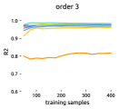
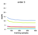
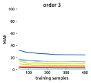
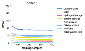
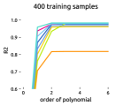
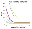
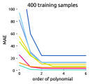
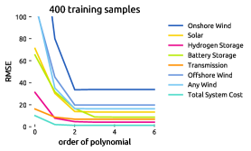
We justify the use of surrogate modelling by cross-validation. Out of the 500 low-fidelity samples, 100 samples are not used in the regression. This validation dataset is unknown to the surrogate model and is consulted to assess the approximation’s quality. Because the high-fidelity sample size is limited and approximating near-optimal solutions is not assumed to fundamentally differ, we base the validation on low-fidelity least-cost solutions only. We experimentally evaluate the approximation errors between predicted and observed data for different combinations of polynomial order and sample size to decide on a suitable parameterisation. We present the coefficient of determination (R²) for the variance captured, the mean absolute (percentage) errors (MAE/MAPE) for absolute and relative deviations, and the root mean squared error (RMSE).

Regarding the number of samples required, Figure 2(a) foremost illustrates that, given enough samples, we achieve average relative errors of less than 4% for most output variables. This is comparable to the cross-validation errors from Tröndle et al. [3] at rates below 5%. Only for offshore wind and battery storage, we observe larger errors. However, this can be explained by a distortion of the relative measure when these technologies are hardly built for some cost projections. On the contrary, the prediction of total system costs is remarkably accurate. Figure 2(a) also demonstrates that for a polynomial order of 3, we gain no significant improvement with more than 200 samples. In fact, thanks to the regularisation term used in the regression, we already attain acceptable levels of accuracy with as few as 50 samples. Moreover, the high R² values underline that the surrogate model can explain most of the output variance.

Regarding the polynomial order, Figure 2(b) shows that an order of 2 and below may be too simple to capture the interaction between different parameters. On the other hand, an order of 4 and above yields no improvement and, were it not for the moderating regularisation term, would even result in a loss of generalisation properties due to overfitting. As higher-order approximations require significantly more samples, an order of 3 appears to be a suitable compromise to limit the computational burden.

3 Results and Discussion

In this section, we approach the uncertainty analysis to near-optimal solutions by reviewing the propagation of input uncertainties into least-cost solutions first and expanding gradually from there. This includes inspecting cost and capacity distributions induced by unknown future technology cost and conducting a global sensitivity analysis that identifies the most influential cost parameters for least-cost solutions. We then expand the uncertainty analysis to the space of nearly cost-optimal solutions, which yields us insights about the consistency of near-optimal alternatives across a variety of cost parameters.

3.1 Cost and Capacity Distribution of Least-Cost Solutions

Figure 3: Distribution of total system cost, generation, storage, and transmission capacities for least-cost solutions.

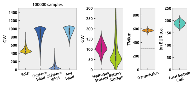
Based on the uncertainty of cost inputs, the total annual system costs vary between 160 and 220 billion Euro per year, as displayed in Figure 3. This means the most pessimistic cost projections entail about 40% higher cost than the most optimistic projections. All least-cost solutions build at least 350 GW solar and 600 GW wind, but no more than 1100 GW. While wind capacities tend towards higher values, solar capacities tend towards lower values. We observe that least-cost solutions clearly prefer onshore over offshore wind, yet onshore wind features the highest uncertainty range alongside battery storage. The cost optimum gravitates towards hydrogen storage rather than battery storage unless battery storage becomes very cheap. There are no least-cost solutions without hydrogen, only some without battery storage. Transmission network expansion is least affected by cost uncertainty and consistently doubled compared to today’s capacities. The question arises, what we can conclude from these insights. The interpretation of the observed ranges may be limited because they are not robust when we look beyond the least-cost solutions and acknowledge structural modelling uncertainties, such as social constraints. Moreover, the pure distribution of outputs does not yet convey information about how sensitive results are to particular cost assumptions. But knowing the technologies for which lowering overnight costs has a significant impact is important to promote technological learning in that direction.

(a) onshore wind

(b) offshore wind

(c) solar

(d) battery storage

(e) hydrogen storage

(f) transmission

Figure 4: Sensitivity of capacities towards their own technology cost. The median (Q50) alongside the 5%, 25%, 75%, and 95% quantiles (Q5–Q95) display the sensitivity subject to the uncertainty induced by other cost parameters.

(a) first-order Sobol indices [%]

(b) total Sobol indices [%]

Figure 5: Sobol indices. These sensitivity indices attribute output variance to random input variables and reveal which inputs the outputs are most sensitive to. The first-order Sobol indices quantify the share of output variance due to variations in one input parameter alone. The total Sobol indices further include interactions with other input variables. Total Sobol indices can be greater than 100% if the contributions are not purely additive.

3.2 Parameter Sweeps and Global Sensitivity Indices

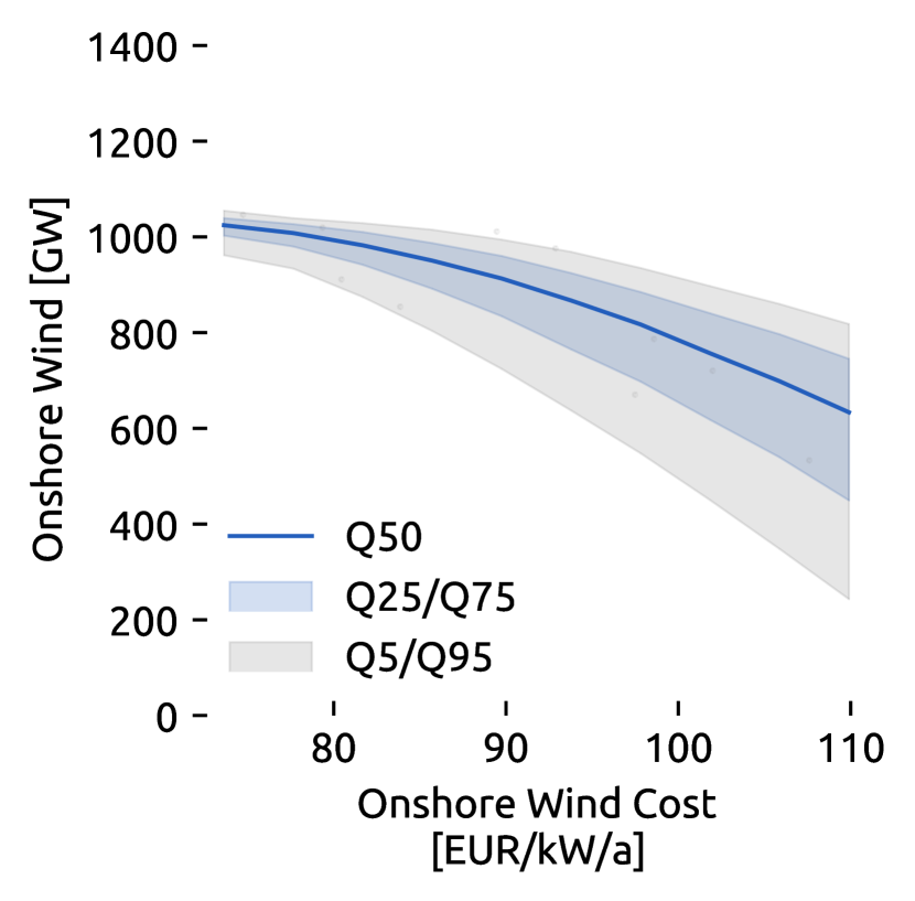
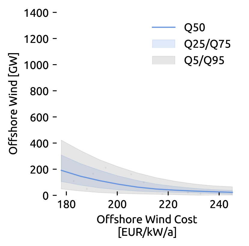
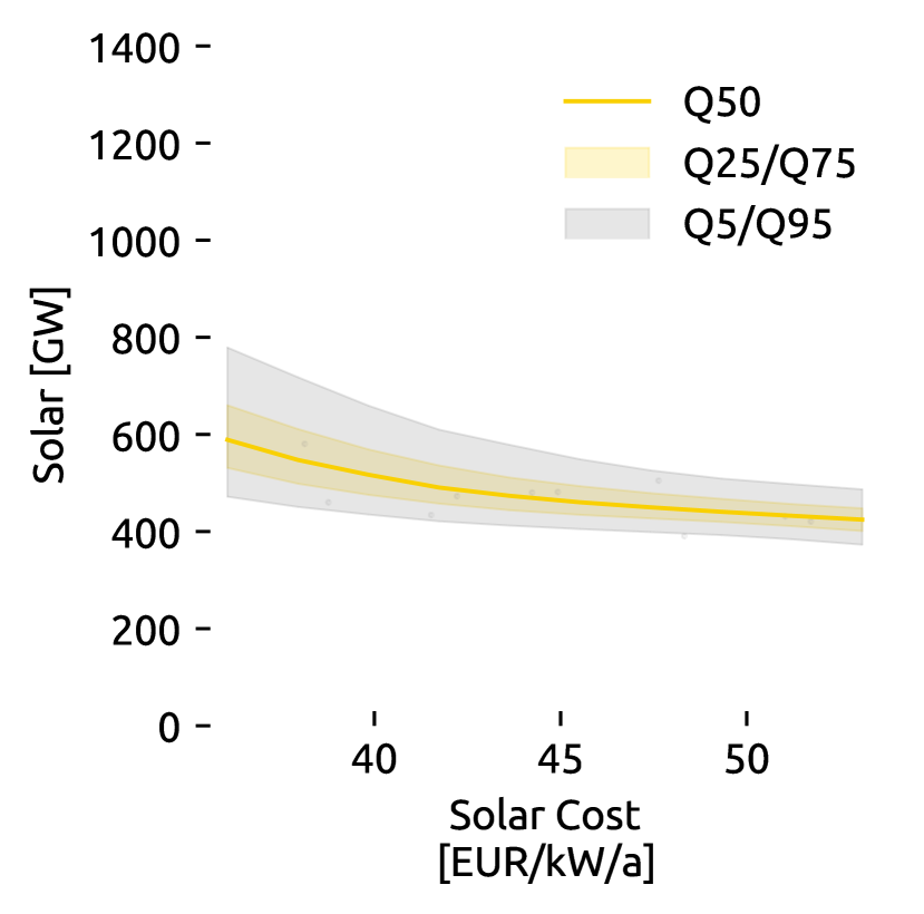
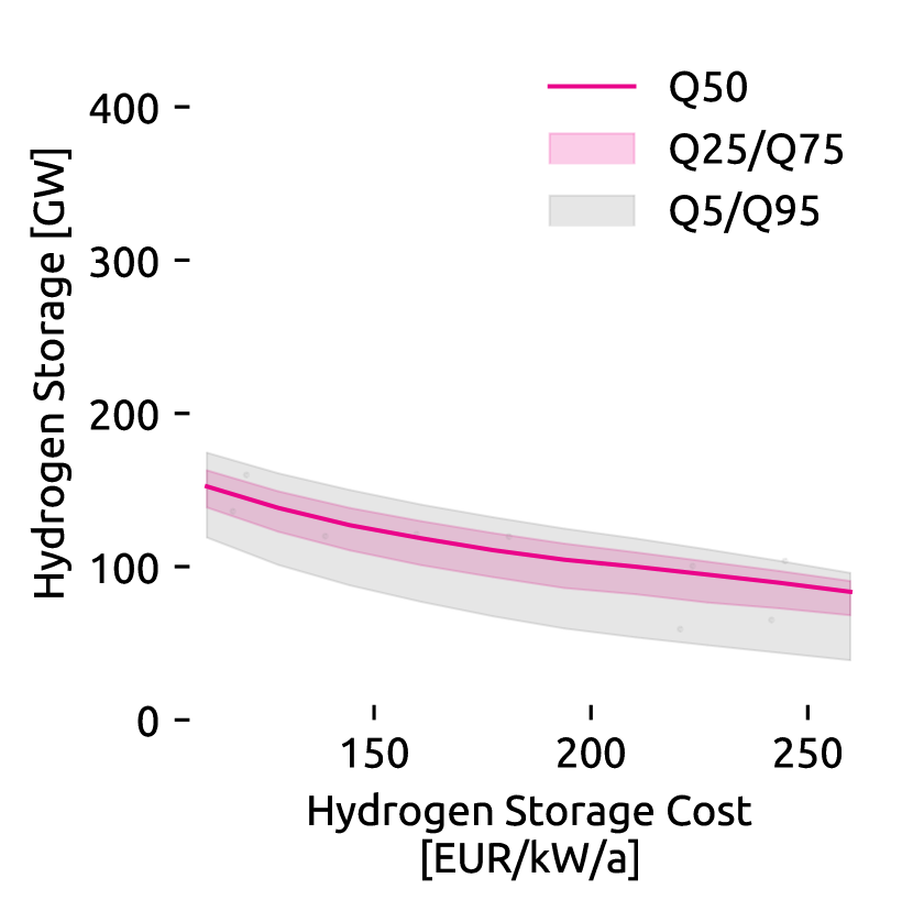
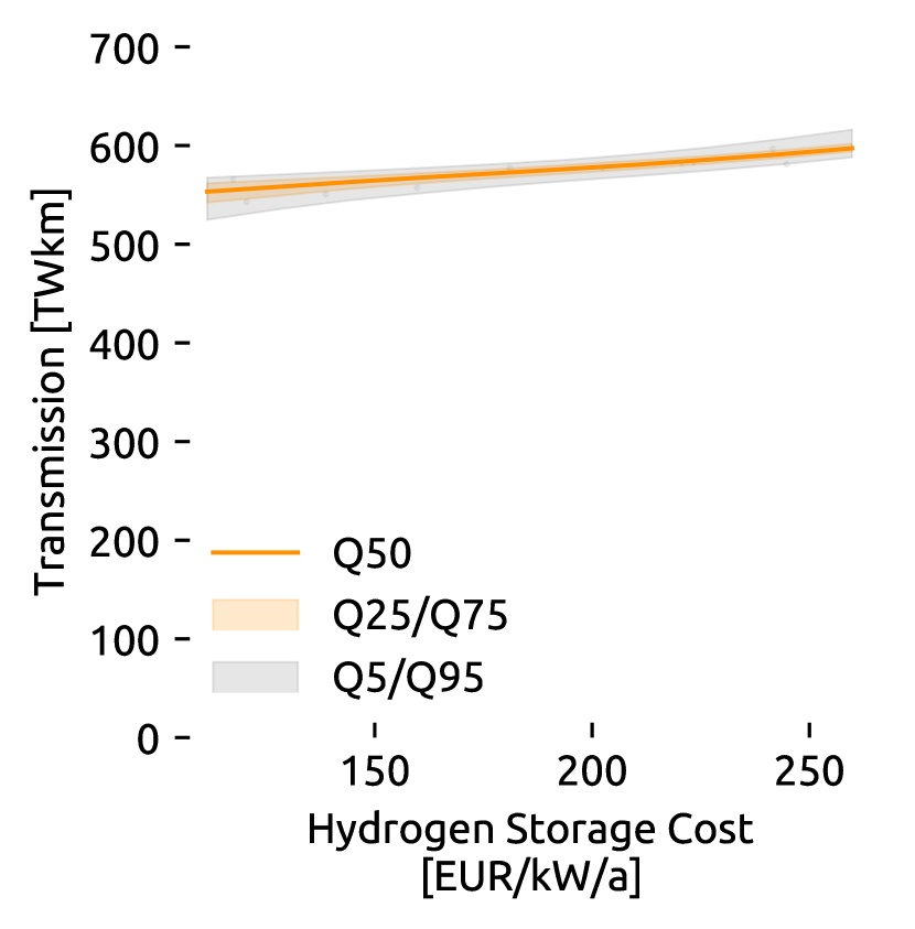
Figure 4 addresses a selection of local self-sensitivities, i.e. how the cost of a technology influences its deployment while displaying the remaining uncertainty induced by other cost parameters. The overall tendency is easily explained: the cheaper a technology becomes, the more it is built. However, changes of slope and effects on the uncertainty range as one cost parameter is swept are insightful nonetheless. For instance, Figure 4 reveals that battery storage becomes significantly more attractive economically once its annuity falls below 75 EUR/kW/a (including 6h energy capacity at full power output) hydrogen storage features a steady slope. A low cost of onshore wind makes building much onshore wind capacity attractive with low uncertainty, whereas if onshore wind costs are high how much is built greatly depends on other cost parameters. The opposite behaviour is observed for offshore wind and solar. The cost of hydrogen storage mostly causes the limited uncertainty about cost-optimal levels of grid expansion. As the cost of hydrogen storage falls, less grid reinforcement is chosen. But since the presented self-sensitivities only exhibit a fraction of all sensitivities, in the next step we formalise how input uncertainties affect each outcome systematically by applying variance-based global sensitivity analysis techniques, which have been applied in the context of energy systems e.g. in [3, 16].

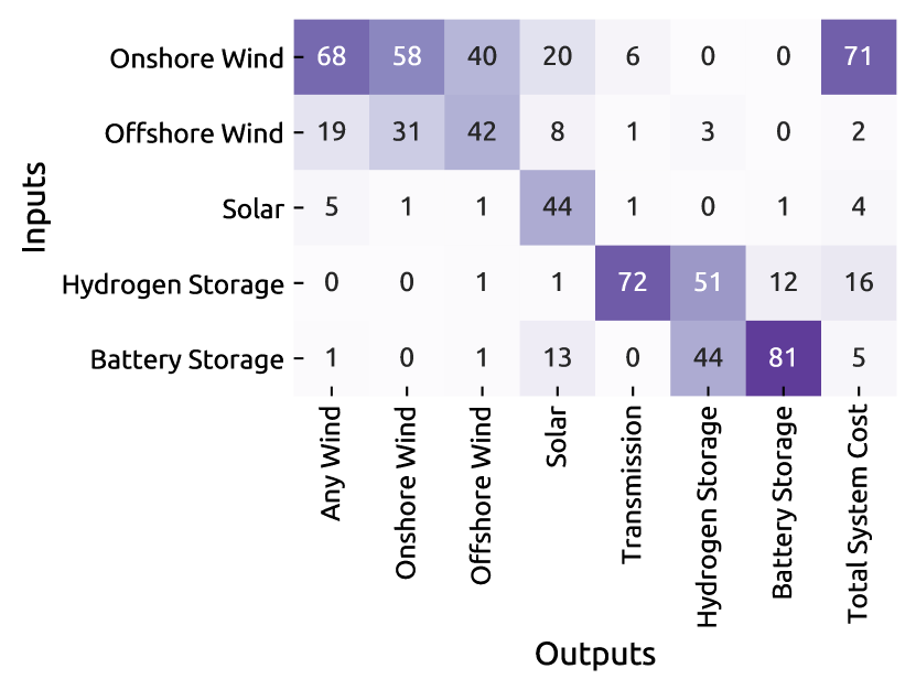
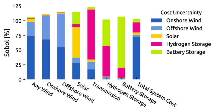
Sensitivity indices, or Sobol indices, attribute the observed output variance to each input and can be computed analytically from the polynomial chaos expansion [38]. For our application, the Sobol indices can, for instance, tell us which technology cost contributes the most to total system cost or how much of a specific technology will be built. The first-order Sobol indices describe the share of output variance due to variations in one input alone averaged over variations in the other inputs. Total Sobol indices also consider higher-order interactions, which are greater than 100% if the relations are not purely additive.

The first-order and total Sobol indices for least-cost solutions in Figure 5 show that the total system cost is largely determined by how expensive it is to build onshore wind capacity, followed by the cost of hydrogen storage. The amount of wind in the system is almost exclusively governed by the cost of onshore and offshore wind parks. Other carriers yield a more varied picture. The cost-optimal solar capacities additionally depend on onshore wind and battery costs. The amount of hydrogen storage is influenced by battery and hydrogen storage cost alike. Although there are noticeable higher-order effects, which are most extensive for transmission, the first-order effects dominate. Strikingly, the volume of transmission network expansion strongly depends on the cost of hydrogen storage, which can be explained by the synoptic spatio-temporal scale of wind power variability across the European continent which both hydrogen storage and transmission networks seek to balance from different angles. While hydrogen storage typically balances multi-week variations in time, continent-spanning transmission networks exploit the circumstance that as weather systems traverse the continent, it is likely always to be windy somewhere in Europe.

3.3 Fuzzy Near-Optimal Corridors with Increasing Cost Slack

So far, we quantified the output uncertainty and analysed the sensitivity towards inputs at least-cost solutions only. Yet, it has been previously shown that even for a single cost parameter set a wide array of technologically diverse but similarly costly solutions exists [6]. In the next step, we examine how technology cost uncertainty affects the shape of the space of near-optimal solutions.

By identifying feasible alternatives common to all, few or no cost samples, we outline low-cost solutions common to most parameter sets (e.g. above 90% contour) as well as system layouts that do not meet low-cost criteria in any circumstances for varying $\epsilon$ in Figure 6. The wider the displayed contour lines are apart, the more uncertainty exists about the boundaries. The closer contour lines are together, the more specific the limits are. The height of the quantiles quantifies flexibility for a given level of certainty and slack; the angle presents information about the sensitivity towards cost slack.

Figure 6: Space of near-optimal solutions by technology under cost uncertainty. For each technology and cost sample, the minimum and maximum capacities obtained for increasing cost penalties $\epsilon$ form a cone, starting from a common least-cost solution. By arguments of convexity, the capacity ranges contained by the cone can be near-optimal and feasible, given a degree of freedom in the other technologies. From optimisation theory, we know that the cones widen up for increased slacks. As we consider technology cost uncertainty, the cone will look slightly different for each sample. The contour lines represent the frequency a solution is inside the near-optimal cone over the whole parameter space. This is calculated from the overlap of many cones, each representing a set of cost assumptions. Due to discrete sampling points in the $\epsilon$-dimension, the plots further apply quadratic interpolation and a Gaussian filter for smoothing.

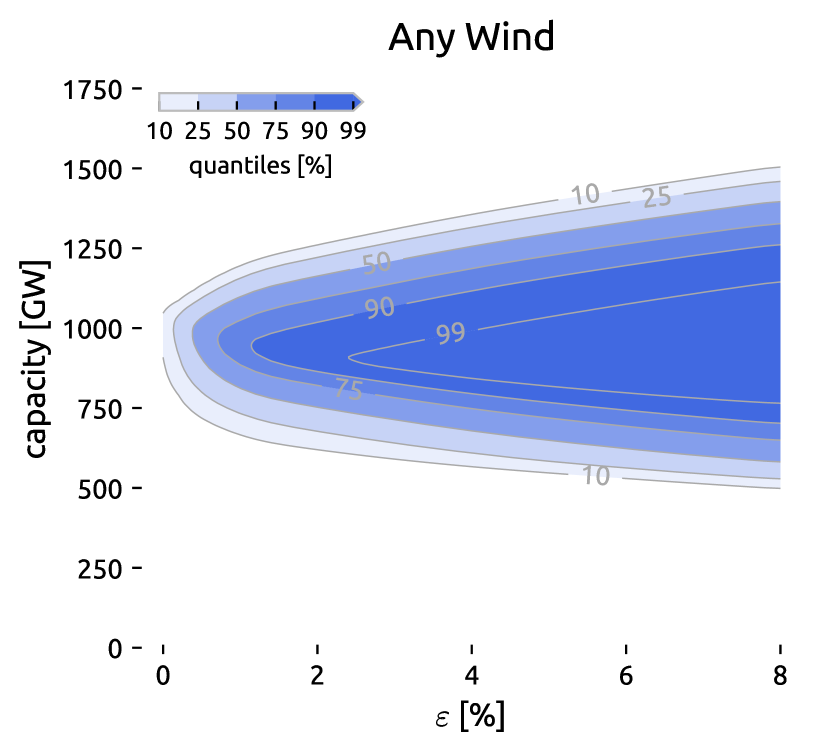
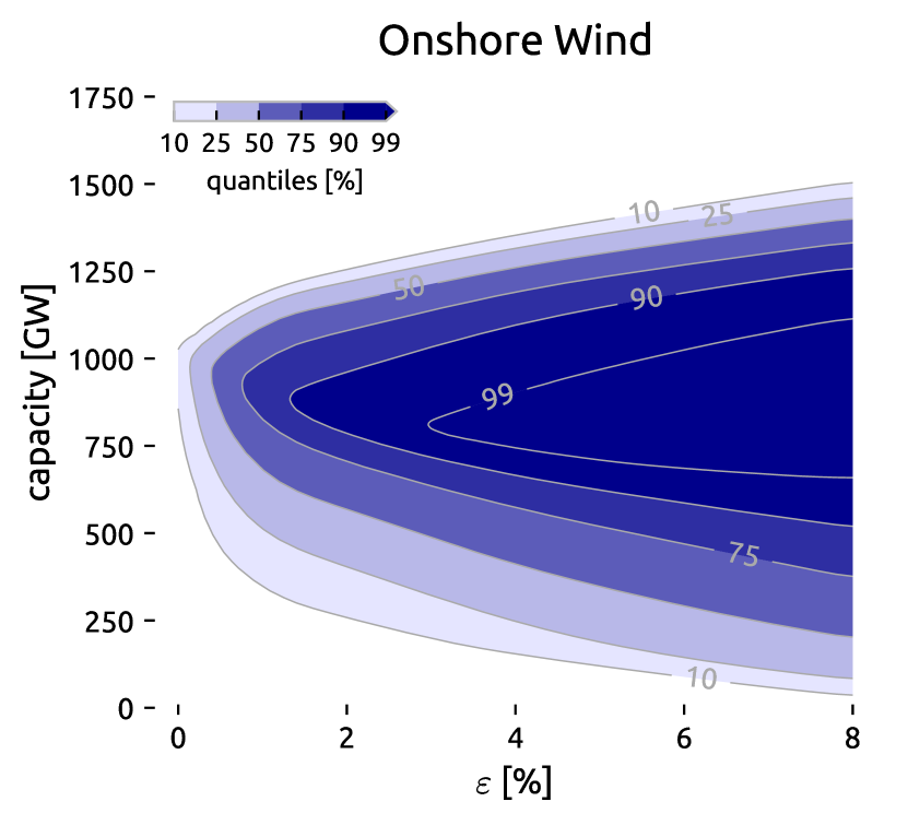
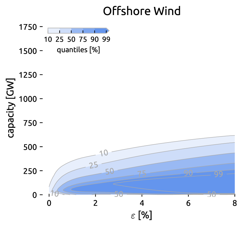
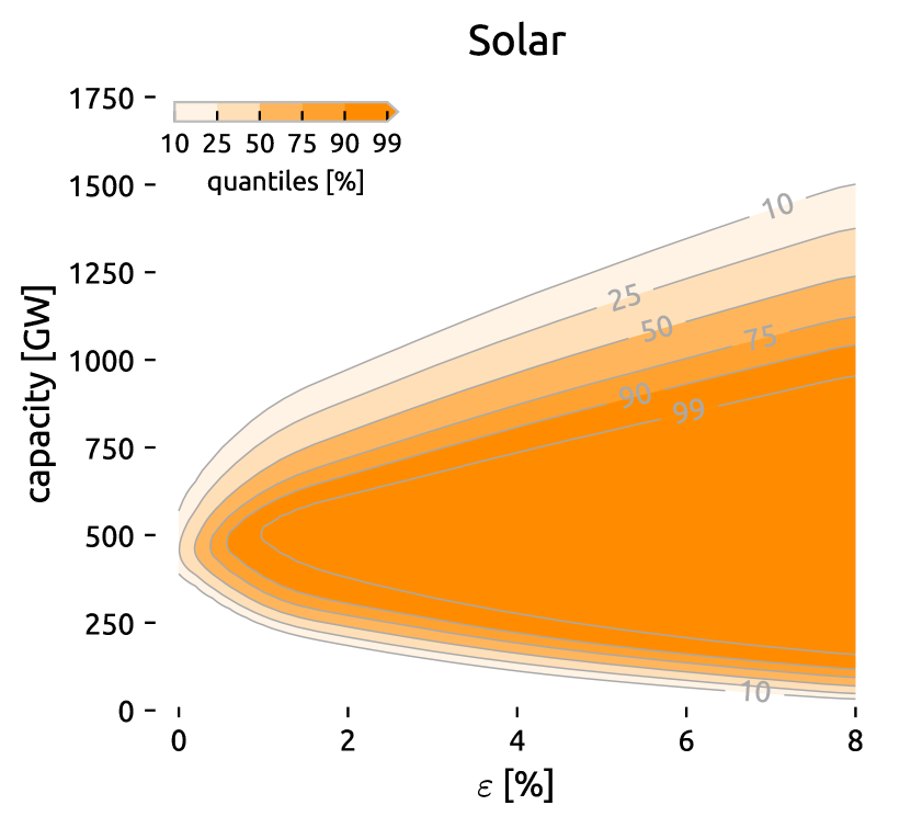
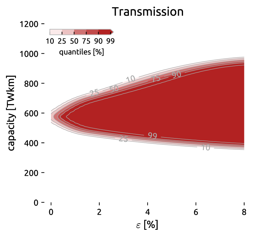
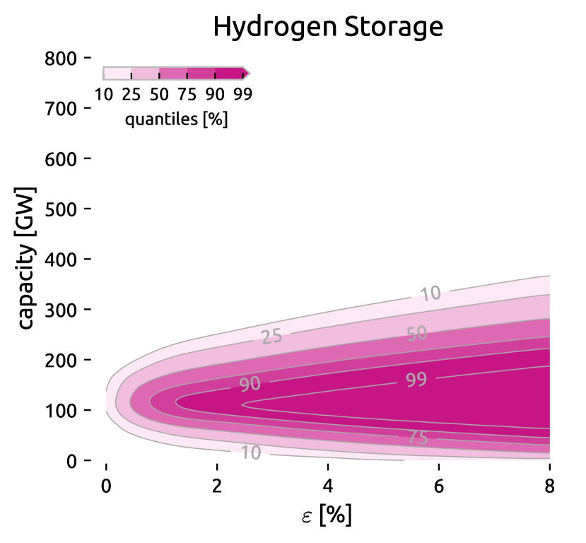
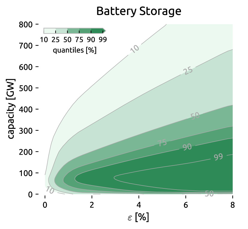
From the fuzzy upper and lower Pareto fronts in Figure 6 we can see that it is highly likely that building 900 GW of wind capacity is possible within 3% of the optimum, and that conversely building less than 600 GW has a low chance of being near the cost optimum. Only a few solutions can forego onshore wind entirely and remain within 8% of the cost-optimum, whereas it is very likely possible to build a system without offshore wind at a cost penalty of 4% at most. On the other hand, more offshore wind generation is equally possible. Unlike for onshore wind, where it is more uncertain how little can be built, uncertainty regarding offshore wind deployment exists about how much can be built so that costs remain within a pre-specified range. For solar, the range of options within 8% of the cost optimum at 90% certainty is very wide. Anything between 100 GW and 1000 GW appears feasible. In comparison to onshore wind, the uncertainty about minimal solar requirements is smaller.

The level of required transmission expansion is least affected by the cost uncertainty. To remain within $\epsilon=8\%$ it is just as likely possible to plan for moderate grid reinforcement by 30% as is initiating extensive remodelling of the grid by tripling the transmission volume compared to what is currently in operation. These results indicate that in any case some transmission reinforcement to balance renewable variations across the continent appears to be essential. Hydrogen storage, symbolising long-term storage, also gives the impression of a vital technology in many cases. Building 100 GW of hydrogen storage capacity is likely viable within 2% of the cost optimum and, even at $\epsilon=8\%$, only 25% of cost samples require no long-term storage; when battery costs are exceptionally low. Overall, 90% of cases appear to function without any short-term battery storage while the system cost rises by 4% at most. However, especially battery storage exhibits a large degree of freedom to build more.

3.4 Probabilistic Near-Optimal Space in Two Technology Dimensions

(a) wind and solar

(b) offshore and onshore wind

(c) hydrogen and battery storage

Figure 7: Space of near-optimal solutions by selected pairs of technologies under cost uncertainty. Just like in Figure 6, the contour lines depict the overlap of the space of near-optimal alternatives across the parameter space. It can be thought of as the cross-section of the probabilistic near-optimal feasible space for a given $\epsilon$ in two technology dimensions and highlights that the extremes of two technologies from Figure 6 cannot be achieved simultaneously.

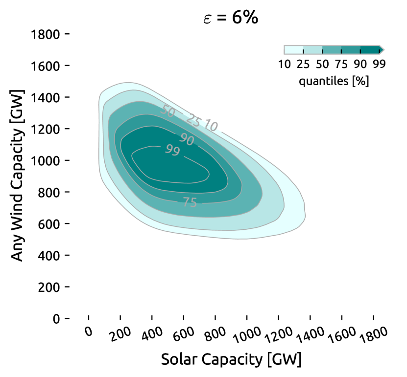
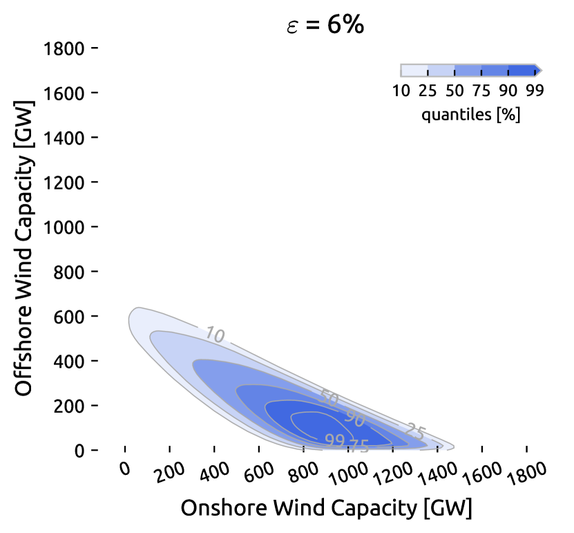
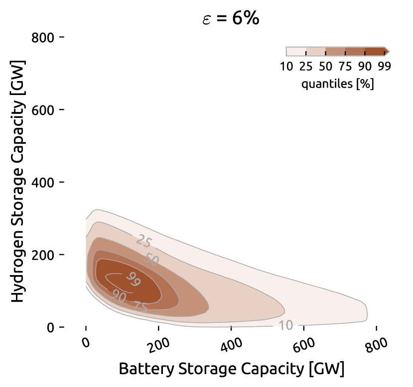
The fuzzy cones from Figure 6 look at trade-offs between system cost and single techologies, assuming that the other technologies can be heavily optimised. But as there are dependencies between the technologies, in Figure 7 we furthermore evaluate trade-offs between technologies for three selected pairs at fixed system cost increase of $\epsilon=6\%$, addressing which combinations of wind and solar capacity, offshore and onshore turbines, and hydrogen and battery storage are likely to be cost-efficient.

First, Figure 7(a) addresses constraints between wind and solar. The upper right boundary exists because building much of both wind and solar would be too expensive. The absence of solutions in the bottom left corner means that building too little of any wind or solar does not suffice to generate enough electricity. From the shape and contours, we see a high chance that building 1000 GW of wind and 400 GW of solar is within 6% of the cost-optimum. On the other hand, building less than 200 GW of solar and 600 GW of wind is unlikely to yield a low-cost solution. In general, minimising the capacity of both primal energy sources will shift capacity installations to high-yield locations even if additional network expansion is necessary and boost the preference for highly efficient storage technologies. Overall, we can take away from this that, even considering combinations of wind and solar, a wide space of low-cost options exists with moderate to high likelihood, although the range of alternatives is shown to be more constrained.

The trade-off between onshore wind and offshore wind is illustrated in Figure 7(b). Here, the most certain area is characterised by building more than 600 GW onshore wind, and less than 250 GW offshore wind capacity. However, there are some solutions with high substitutability between onshore and offshore wind, shown in the upper left bulge of the contour plot. Compared to wind and solar, the range of near-optimal solutions is even more constrained. The key role of energy storage in a fully renewable system is underlined in Figure 7(c). Around 50 GW of each is at least needed in any case, while highest likelihoods are attained when building 150 GW of each.

(a) minimal onshore wind with 8% system cost slack

(b) minimal transmission expansion with 8% system cost slack

Figure 8: Distribution of total system cost, generation, storage, and transmission capacities for two near-optimal search directions with $\epsilon=8\%$ system cost slack.

3.5 Capacity Distributions at Minimal Onshore Wind and Transmission Grid

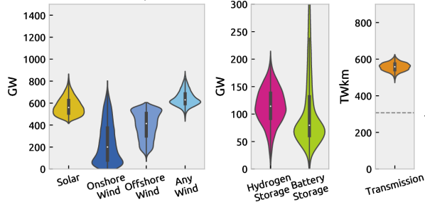
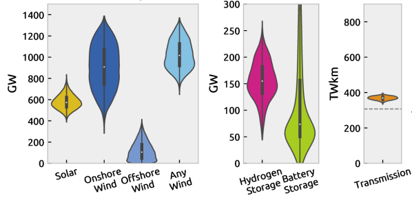
The aforementioned contour plots Figures 6 to 7 outline what is likely possible within specified cost ranges and subject to technology cost uncertainty, but do not expose the changes the overall system layout experiences when reaching for the extremes in one technology. Therefore, we show in Figure 8 how the system-wide capacity distributions vary compared to the least-cost solutions (Figure 3) for two exemplary alternative objectives. For that, we chose minimising onshore wind capacity and transmission expansion because they are often linked to social acceptance issues.

Figure 8(a) illustrates that reducing onshore wind capacity is predominantly compensated by increased offshore wind generation but also added solar capacities. The increased focus on offshore wind also leads to a tendency towards more hydrogen storage, while transmission expansion levels are similarly distributed as for the least-cost solutions. From Figure 8(b) we can further extract that avoiding transmission expansion entails more hydrogen storage that compensates balancing in space with balancing in time, and more generation capacity overall, where resources are distributed to locations with high demand but weaker capacity factors and more heavily curtailed.

3.6 Critical Appraisal

The need to solve models for many cost projections and near-optimal search directions in reasonable time means that compromises had to be made in other modelling dimensions. For instance, the analysis would profit from a richer set of technologies and further uncertain input parameters, including efficiencies of fuel cells and electrolysis or the consideration of concentrating solar power, geothermal energy, biomass, and nuclear to name just a few. But as the number of considered technologies and parameters rises, so does the computational burden. Given the already considerable computational efforts involved in procuring our results, considering the full breadth of technologies and uncertainties would not have been feasible with the computational resources available. Moreover, limitations apply to the scope of the analysis which is limited to the electricity sector does not consider coupling to other energy sectors. However, accounting for interactions across sectors at high resolution in similarly set future studies is desirable and in development. Additionally, we assess no path dependencies via multi-period investments and endogenous learning, but optimise for an emission reduction in a particular target year based on annualised costs. We further disregard interannual variations of weather data by basing the analysis just on a single weather year for computational reasons. Lastly, aspects such as reserves, system adequacy and inertia have not been considered.

4 Conclusion

In this work, we systematically explore a space of alternatives beyond least-cost solutions for society and politics to work with. We show how narrowly following cost-optimal results underplays an immense degree of freedom in designing future renewable power systems. To back our finding that there is no unique path to cost-efficiency, we account for the inherent uncertainties regarding technology cost projections, and draw robust conclusions about the range of options, boundary conditions and cost sensitivities:

Wide Range of Trade-Offs

We find that there is a substantial range of options within 8% of the least-cost solution regardless of how cost developments will unfold. This holds across all technologies individually and even when considering dependencies between wind and solar, offshore and onshore wind, as well as hydrogen and battery storage.

Must-Avoid Boundary Conditions

We also carve out a few boundary conditions which must be met to keep costs low and are not affected by the prevailing cost uncertainty. For a fully renewable power system, either offshore or onshore wind capacities in the order of 600 GW along with some long-term storage technology and transmission network reinforcement by more than 30% appears essential.

Technology Cost Sensitivities

We identify onshore wind cost as the apparent main determinant of system cost, though it can often be substituted with offshore wind for a small additional cost. Moreover, the deployment of batteries is the most sensitive to its cost, whereas required levels of transmission expansion are least affected by cost uncertainty.

The robust investment flexibility in shaping a fully renewable power system we reveal opens the floor to discussions about social trade-offs and navigating around issues, such as public opposition towards wind turbines or transmission lines. Rather than modellers making normative choices about how the energy system should be optimised, we offer methods that present a wide spectrum of options and trade-offs that are feasible and within a reasonable cost range, to help society decide how to shape the future of the energy system.

CRediT Author Statement

Fabian Neumann: Conceptualization, Methodology, Investigation, Software, Validation, Formal analysis, Visualization, Writing – Original Draft, Writing – Review & Editing Tom Brown: Conceptualization, Writing – Review & Editing, Supervision, Project administration, Funding acquisition

Data Availability

The code to reproduce the experiments is available at github.com/fneum/broad-ranges. We also refer to the documentation of PyPSA (pypsa.readthedocs.io) and PyPSA-Eur (pypsa-eur.readthedocs.io).

References

- [1] E. Trutnevyte, Does cost optimization approximate the real-world energy transition?, Energy 106 (2016) 182–193. doi:10/f8vrcz.
- [2] S. Pye, O. Broad, C. Bataille, P. Brockway, H. E. Daly, R. Freeman, A. Gambhir, O. Geden, F. Rogan, S. Sanghvi, J. Tomei, I. Vorushylo, J. Watson, Modelling net-zero emissions energy systems requires a change in approach, Climate Policy (2020) 1–10doi:10/ghdkp9.
- [3] T. Tröndle, J. Lilliestam, S. Marelli, S. Pfenninger, Trade-Offs between Geographic Scale, Cost, and Infrastructure Requirements for Fully Renewable Electricity in Europe, Joule (2020) S2542435120303366doi:10/gg8zk2.
- [4] X. Yue, S. Pye, J. DeCarolis, F. G. Li, F. Rogan, B. O. Gallachòir, A review of approaches to uncertainty assessment in energy system optimization models, Energy Strategy Reviews 21 (2018) 204–217. doi:10/gf75x4.
- [5] S. Pye, F. G. Li, A. Petersen, O. Broad, W. McDowall, J. Price, W. Usher, Assessing qualitative and quantitative dimensions of uncertainty in energy modelling for policy support in the United Kingdom, Energy Research & Social Science 46 (2018) 332–344. doi:10/gf8nvv.
- [6] F. Neumann, T. Brown, The near-optimal feasible space of a renewable power system model, Electric Power Systems Research 190 (2021) 106690, arXiv:1910.01891. doi:10/ghcpr2.
- [7] F. Lombardi, B. Pickering, E. Colombo, S. Pfenninger, Policy Decision Support for Renewables Deployment through Spatially Explicit Practically Optimal Alternatives, Joule (2020) S2542435120303482doi:10/gg8z6v.
- [8] J.-P. Sasse, E. Trutnevyte, Regional impacts of electricity system transition in Central Europe until 2035, Nature Communications 11 (1) (2020) 4972. doi:10/ghdwjs.
- [9] D. L. McCollum, A. Gambhir, J. Rogelj, C. Wilson, Energy modellers should explore extremes more systematically in scenarios, Nature Energy 5 (2) (2020) 104–107. doi:10/ggk3hj.
- [10] D. P. Schlachtberger, T. Brown, M. Schäfer, S. Schramm, M. Greiner, Cost optimal scenarios of a future highly renewable European electricity system: Exploring the influence of weather data, cost parameters and policy constraints, Energy 163 (2018) 100–114. doi:10/gfk5cj.
- [11] J. F. DeCarolis, S. Babaee, B. Li, S. Kanungo, Modelling to generate alternatives with an energy system optimization model, Environmental Modelling and Software 79 (2016) 300–310. doi:10/f8n923.
- [12] F. G. Li, E. Trutnevyte, Investment appraisal of cost-optimal and near-optimal pathways for the UK electricity sector transition to 2050, Applied Energy 189 (2017) 89–109. doi:10/f9qtrf.
- [13] L. Nacken, F. Krebs, T. Fischer, C. Hoffmann, Integrated renewable energy systems for Germany – A model-based exploration of the decision space, 2019, p. 8.
- [14] J. Price, I. Keppo, Modelling to generate alternatives: A technique to explore uncertainty in energy-environment-economy models, Applied Energy 195 (2017) 356–369. doi:10/ggfzqq.
- [15] T. T. Pedersen, M. Victoria, M. G. Rasmussen, G. B. Andresen, Modeling all alternative solutions for highly renewable energy systems, arXiv:2010.00836 (Oct. 2020).
- [16] G. Mavromatidis, K. Orehounig, J. Carmeliet, Uncertainty and global sensitivity analysis for the optimal design of distributed energy systems, Applied Energy 214 (2018) 219–238. doi:10/gc6n48.
- [17] A. Pizarro-Alonso, H. Ravn, M. Münster, Uncertainties towards a fossil-free system with high integration of wind energy in long-term planning, Applied Energy 253 (2019) 113528. doi:10/ghfgtx.
- [18] B. Fais, I. Keppo, M. Zeyringer, W. Usher, H. Daly, Impact of technology uncertainty on future low-carbon pathways in the UK, Energy Strategy Reviews 13-14 (2016) 154–168. doi:10/f9gmpd.
- [19] W. Usher, The Value of Global Sensitivity Analysis for Energy System Modelling (2015) 29.
- [20] J. Hörsch, H. Ronellenfitsch, D. Witthaut, T. Brown, Linear optimal power flow using cycle flows, Electric Power Systems Research 158 (2018) 126–135, arXiv:1704.01881. doi:10/gdb8kx.
- [21] T. Brown, J. Hörsch, D. Schlachtberger, PyPSA: Python for Power System Analysis, Journal of Open Research Software 6 (2018) 4, arXiv:1707.09913. doi:10/gfb7m9.
- [22] G. Mavrotas, Effective implementation of the -constraint method in Multi-Objective Mathematical Programming problems, Applied Mathematics and Computation 213 (2) (2009) 455–465. doi:10/bwkzrt.
- [23] J. Hörsch, F. Hofmann, D. Schlachtberger, T. Brown, PyPSA-Eur: An open optimisation model of the European transmission system, Energy Strategy Reviews 22 (2018) 207–215, arXiv:1806.01613. doi:10/d294.
- [24] J. Köster, S. Rahmann, Snakemake—a scalable bioinformatics workflow engine, Bioinformatics 28 (19) (2012) 2520–2522. doi:10/gd2xzq.
-
[25]
Danish Energy Agency,
Technology
data (2020).
URL https://ens.dk/en/our-services/projections-and-models/technology-data - [26] A. Gritsevskyi, N. Nakićenovi, Modeling uncertainty of induced technological change, Energy Policy 28 (13) (2000) 907–921. doi:10/d4rkhb.
- [27] S. Yeh, E. S. Rubin, A review of uncertainties in technology experience curves, Energy Economics 34 (3) (2012) 762–771. doi:10/dzc2b4.
- [28] C. F. Heuberger, E. S. Rubin, I. Staffell, N. Shah, N. Mac Dowell, Power capacity expansion planning considering endogenous technology cost learning, Applied Energy 204 (2017) 831–845. doi:10/gcgs2v.
- [29] N. Mattsson, Learning by modeling energy systems, Ph.D. thesis (2019).
- [30] S. Moret, V. Codina Gironès, M. Bierlaire, F. Maréchal, Characterization of input uncertainties in strategic energy planning models, Applied Energy 202 (2017) 597–617. doi:10/gbsxmz.
- [31] B. Shirizadeh, Q. Perrier, P. Quirion, How sensitive are optimal fully renewable power systems to technology cost uncertainty? (2019) 45.
- [32] P.-H. Li, S. Pye, I. Keppo, Using clustering algorithms to characterise uncertain long-term decarbonisation pathways, Applied Energy 268 (2020) 114947. doi:10/ghchgg.
- [33] S. Moret, M. Bierlaire, F. Maréchal, Robust Optimization for Strategic Energy Planning, Informatica 27 (3) (2016) 625–648. doi:10/f87mh8.
- [34] S. Pilpola, P. D. Lund, Analyzing the effects of uncertainties on the modelling of low-carbon energy system pathways, Energy 201 (2020) 117652. doi:10/ggtk2r.
- [35] E. Trutnevyte, EXPANSE methodology for evaluating the economic potential of renewable energy from an energy mix perspective, Applied Energy 111 (2013) 593–601. doi:10/ftdb.
- [36] Lopion, Markewitz, Stolten, Robinius, Cost Uncertainties in Energy System Optimization Models: A Quadratic Programming Approach for Avoiding Penny Switching Effects, Energies 12 (20) (2019) 4006. doi:10/ghchff.
- [37] P. S. Palar, T. Tsuchiya, G. T. Parks, Multi-fidelity non-intrusive polynomial chaos based on regression, Computer Methods in Applied Mechanics and Engineering 305 (2016) 579–606. doi:10/f8jsb6.
- [38] B. Sudret, Global sensitivity analysis using polynomial chaos expansions, Reliability Engineering & System Safety 93 (7) (2008) 964–979. doi:10/bjjp5r.
- [39] N. Fajraoui, S. Marelli, B. Sudret, On optimal experimental designs for Sparse Polynomial Chaos Expansions, arXiv:1703.05312 (Mar. 2017).
- [40] L. L. Gratiet, S. Marelli, B. Sudret, Metamodel-based sensitivity analysis: Polynomial chaos expansions and Gaussian processes, arXiv:1606.04273 (2015) 1–37doi:10/ggxtbp.
- [41] T. Mühlpfordt, Uncertainty Quantification via Polynomial Chaos Expansion – Methods and Applications for Optimization of Power Systems (2020). doi:10/ggxtbr.
- [42] J. Feinberg, H. P. Langtangen, Chaospy: An open source tool for designing methods of uncertainty quantification, Journal of Computational Science 11 (2015) 46–57. doi:10/gddwzk.
- [43] L. W.-T. Ng, M. Eldred, Multifidelity Uncertainty Quantification Using Non-Intrusive Polynomial Chaos and Stochastic Collocation, in: 53rd AIAA/ASME/ASCE/AHS/ASC Structures, Structural Dynamics and Materials Conference, American Institute of Aeronautics and Astronautics, Honolulu, Hawaii, 2012. doi:10/ghknms.
- [44] S. Hosder, R. Walters, M. Balch, Efficient Sampling for Non-Intrusive Polynomial Chaos Applications with Multiple Uncertain Input Variables. doi:10/ftdc.