Towards Eliciting Weak or Incomplete Preferences in the Lab:
A Model-Rich Approach

Abstract

Recovering and distinguishing between the potentially meaningful indifference and/or indecisiveness parts of a decision maker’s preferences from their observable choice behaviour is important for testing theory and conducting welfare analysis. This paper contributes a way forward in two ways. First, it reports on a new experimental design with a forced and a non-forced general choice treatment where the 282 subjects in the sample were allowed to choose multiple gift-card bundles from each menu they saw. Second, it analyses the collected data with a new non-parametric combinatorial-optimization method that allows to compare the goodness-of-fit of utility maximization to that of models of undominated or dominant choice with incomplete preferences, in each case with or without indifferences. Most subjects in the sample are well-approximated by some indifference-permitting instance of those three models. Furthermore, the model-specific preference recovery typically elicits a unique preference relation with a non-trivial indifference part and, where relevant, a distinct indecisiveness part. The two kinds of distinctions between indifference and indecisiveness uncovered herein are theory-guided and documented empirically for the first time. Our findings suggest that accounting for the decision makers’ possible indifference or inability to compare some alternatives can increase the descriptive accuracy of theoretical models and their empirical tests thereof, while it can also aid attempts to recover people’s stable but possibly weak or incomplete preferences.

Keywords:
Multi-valued choice experiment; indifference elicitation; incomplete-preference elicitation; revealed indifference vs revealed indecisiveness; combinatorial optimization; goodness of fit.

1         Introduction

The state in which a decision maker is indifferent between two or more choice alternatives plays a prominent role in many domains of economic analysis. As such, it is important to understand the kinds of observable decision environments and data-analytic methods that can in principle allow for extracting an individual’s potentially weak preferences and distinguishing between their strict-preference and indifference parts. This is particularly so if one also accepts that the individual in question may be indecisive, with preferences that are transitive but potentially incomplete. In this situation, it is unclear how such observable decision data could be used to separate indifference from incomparability/indecisiveness.

These problems are important, both from a theoretical and a policy perspective. Indeed, since many economic models of individual, collective or interactive decisions assume that agents have preferences with non-trivial indifference parts, elicitation of the agents’ weak preference relations would allow for testing these models’ descriptive relevance more accurately than if indifferences were assumed away. Additionally, knowing how many decision makers within a community consider a tree-planting program to be equally good to the development of a playground, for example, and how many of them have a strict preference instead would generally allow the community leader to arrive at a better decision than if all preferences were mistakenly interpreted to be strict. This example is made more concrete in the table below, which shows how eliciting single choices in the presence of indifferences may lead to a Pareto inefficient social outcome while eliciting multiple choices would not:

	Anna	Basel	Cora	Majority-rule
				preference/choice
True preferences	$TreePlanting$	$TreePlanting$	$TreePlanting$
	$\succ_{A}$	$\sim_{B}$	$\sim_{C}$	$TreePlanting$
	$PlayGround$	$PlayGround$	$PlayGround$
Multiple choices not allowed	$TreePlanting$	$PlayGround$	$PlayGround$	$PlayGround$
(single choices observed with positive probability)
Multiple choices allowed	$TreePlanting$	$TreePlanting$	$TreePlanting$	$TreePlanting$
(choices observed with certainty)		&	&
		$PlayGround$	$PlayGround$

Similarly, understanding when agents are indifferent and when they are indecisive can enable the policy maker to understand whether they should immediately make an active choice that will impact everyone in the group or delay such a choice and aim instead to inform the group’s members towards resolving their indecisiveness, e.g. via targeted information campaigns.

This paper’s first contribution is to propose and apply an incentivized lab experimental design which elicits observable behavioural data that could be used to recover an individual’s weak preferences and distinguish between their strict part, indifference part and, where relevant, incomparability/indecisiveness part. The main feature of the design is that it allows subjects to make multiple choices from every menu of alternatives they see by introducing incentives that help them make such possibly multi-valued choices in a preference-guided way. Subjects in the Non-Forced-Choice treatment can additionally avoid/delay making a choice from any menu at a small cost, and without receiving any additional information about the alternatives. Subjects in the Forced-Choice treatment on the other hand are always required to choose at least one option. This experimental design was implemented in an environment of riskless choice from 50 distinct menus that were derived from 6 pairs of popular £10 gift cards, and data from 282 subjects were collected.

The second contribution consists of analysing these data by applying an optimization-based computational method that allows for a model-rich approach towards recovering an individual’s potentially weak and/or incomplete preferences. This method builds on and extends in a model-based way the classic Houtman and Maks (1985) technique that is routinely used in empirical revealed preference tests of the rational choice/utility maximization hypothesis. More specifically, the original Houtman-Maks technique computes the maximal subset of a subject’s dataset that is consistent with rational choice, essentially allowing for an intuitive quantification of the subject’s behavioural proximity with that model. The extension that we use applies this approximation principle simultaneously to the model of rational choice and two additional models of incomplete-preference maximization: (i) undominated choice, whereby an individual chooses the feasible alternative(s) that are not worse than anything else; (ii) dominant choice, whereby they choose the most preferred feasible alternative(s) if and only if those exist and defer otherwise. Consistent with the questions that we raised earlier, all three models predict multi-valued choices under some of their admissible preference orderings, while the latter two also afford or predict two theoretical separations between revealed indifference and incomparability/indecisiveness. By finding which model is closest to explaining each subject’s behaviour, this method effectively allows for recovering –possibly approximately, and with the standard as if qualifications in place– both the individual’s deterministic decision rule and their preferences conditional on this rule.

Turning to our main empirical findings at the individual level, despite the relatively large number of experimental decisions, 56% of all subjects are well-explained by one of the above three models of preference maximization, while the model-optimally recovered preferences of 72% of all subjects in this group feature at least one indifference comparison between distinct alternatives. As far as the decomposition of preference-maximization types is concerned, 35% and 21% of all subjects are best matched by utility maximization and the two models of incomplete-preference maximization, respectively, and a single optimal preference relation is recovered from 86% of all these subjects. Importantly, the preferences elicited from nearly two thirds of all incomplete-preference maximizers document empirically –and for the first time– the distinct theoretical separations between revealed indifference and revealed indecisiveness that are afforded by the two relevant models. Both these separations assume the analyst has access to the kind of multi-valued choice data that we elicit in this paper. The above findings therefore highlight the potential usefulness of multi-valued choice data, indifference-permitting deterministic models of complete and incomplete preferences, and combinatorial-optimization goodness-of-fit methods of testing them.

At the aggregate level, we find a significant –and nearly identical– negative correlation between subjects’ choice consistency and their average response times. Although seemingly counter-intuitive, this interesting finding is broadly in line with a key prediction of the influential drift-diffusion neuro-economic model (see Ratcliff and McCoon, 2008). The prediction might be interpreted as suggesting that shorter response times are more likely when the decision maker has a clear preference between the feasible options. Such clarity in turn would be expected to translate into more consistent active choices, which is indeed what we find. In addition, and despite the fact that subjects in our experiment were allowed to –and typically did– make multi-valued instead of single-valued choices, those in the Non-Forced-Choice treatment behaved significantly more consistently. We therefore provide a positive robustness check of the main finding in the study by Costa-Gomes, Cueva, Gerasimou, and Tejiščák (2022), which was designed to test for such potential differences in consistency with single-choice data.

Although not constructed so as to enable a thorough investigation of such behaviours, we also note that utilizing two important aspects of the experimental design and its implementation allows for inferring that an additional 10% of the analysed subjects could be thought of as exhibiting systematic satisficing behaviour (Simon, 1956; Caplin et al., 2011; Reutskaja et al., 2011) or a preference for randomization (Agranov and Ortoleva, 2017, 2023; Dwenger et al., 2018; Agranov et al., 2022). Together with the model-based findings mentioned above, this increases the total proportion of behaviourally explainable subjects in our data to 66%.

Finally, although our experimental design is applicable in the lab and also in online surveys, we also note that non-forced and/or multi-valued choice data could in principle be collected in real-world environments as well. For example, an online retailer may analyse the decisions of a customer who repeatedly makes use of the retailer’s generous returns policy by buying multiple products with every order and then returning all but one for a full refund. In this case the seller knows all menus seen by that customer, the set of products they bought in each case, and the one they finally kept. Similarly, the retailer may analyse data from another customer who often browses the products in various menus but ultimately decides to buy none.

The remaining part of the paper is organized as follows. The next section presents the experimental design and its implementation. Section 3 discusses the main aggregate-level findings on subjects’ behaviour across the two treatments. Section 4 –the heart of the paper– proceeds with the individual-level analysis and the recovery of subjects’ decision rules, preferences and heuristics. Online Appendices A–D contain additional information about the experimental design, data analysis and recovered preference relations.

2         Experimental Design

2.1         Structure

We describe the Forced-Choice treatment design first. At the beginning of the experiment subjects are allocated a monetary endowment $I>0$. In the main part they are presented sequentially with a series of menus of choice alternatives. When a menu is shown, subjects are asked to choose one or more items from that menu. Subjects know that one menu will be picked at random for them at the end of the experiment. They also know that they will be rewarded with an element of their randomly selected menu, and that the decision they made at that menu during the main part of the experiment will be reminded to them before they are asked to make their final, payoff-relevant decision there. Once subjects are past a menu during the main part of the experiment they never see it again unless that menu later turns out to be their randomly selected one. No information about the choice alternatives is provided at any point.

If a Forced-Choice subject chooses one or more -but not all- options from their randomly selected menu during the main part of the experiment, and also chooses something from those previously selected options if that menu is determined to be their payoff-relevant one, then they receive that item as an in-kind reward and $I$ as a cash reward. If, instead, they now choose something that is not among their previously chosen options at that menu, then they receive that item and a positive amount $I_{rev}<I$. Finally, if they had chosen everything at that menu originally, then they receive their original endowment $I$ and a randomly selected element of that menu.

Denoting by $A$ a subject’s payoff-relevant randomly selected menu, and by $C^{1}(A)$, $C^{2}(A)$ the choices they made at that menu during the main and final parts, respectively, Table 1 summarizes the incentive structure in this treatment. Under the assumption of a utility-maximizing decision maker with possibly weak preferences, $C^{1}(\cdot)$ denotes their nonempty- but possibly multi-valued choice correspondence. That is, for a Forced-Choice subject $C^{1}(\cdot)$ satisfies $\emptyset\neq C^{1}(M)\subseteq M$ for every menu $M$. By contrast, $C^{2}(A)$ assigns a single chosen alternative to the subject’s randomly selected menu $A$.

By the very definition of indifference, a utility-maximizing subject who operates under this Forced-Choice design and is indifferent between all feasible alternatives at a menu is also indifferent between choosing all these alternatives or any sub-collection of them. Hence, such a subject has no strict incentive to misreport their indifference. Conversely, however, they will choose everything in a menu only if they are indifferent between all alternatives at that menu because, by definition of indifference, this individual does not care which alternative they will get or whether this is decided by someone else or randomly (see also Danan (2010) for a formal elaboration of this point). Thus, it is weakly dominant for this subject to choose everything feasible in a menu whenever they are indifferent between all items contained in it. On the other hand, if a utility-maximizing subject has one or more optimal alternative(s) at the menu, and these are strictly better than something else feasible, then choosing everything is dis-incentivized by the design because doing so comes with the risk of potentially receiving an inferior alternative as a reward. The design instead incentivizes such a subject to select those and only those options they prefer the most, as this enables them to choose one of these superior options at the end and also receive their full cash endowment. For a utility-maximizing agent, therefore, the design in this treatment novelly combines incentive-compatibility for truthful preference revelation in the sense of Azrieli et al. (2018) with a standard interpretation of multi-valued choice that is articulated in Kreps (2012, p.2) as follows: “The story is that the consumer chooses one element of $A$. Nonetheless, we think of $c(A)$ as a subset of $A$, not a member or element of $A$. This allows for the possibility that the consumer is happy with any one of the several elements of $A$, in which case $c(A)$ lists all those elements. When she makes a definite choice of a single element, say $x$, out of $A$–when she says in effect, ‘I want $x$ and nothing else’–we write $c(A)=\{x\}$, or the singleton set consisting of the single element $\{x\}$. But if she says, ‘I would be happy with either $x$ or $y$’, then $c(A)=\{x,y\}$.”

What if a subject in this Forced-Choice treatment has stable and transitive but incomplete preferences, and does not have a most preferred option at some menu? It is clear from the above that the design dis-incentivizes choice of preference-dominated options. Anticipating the discussion of Section 4.1 below, it is then possible that the multi-valued choice $C^{1}(A)$ of some such subject would reveal the set of undominated alternatives at menu $A$ between which the agent is either indifferent or indecisive.

Table 1: Incentives in both the Forced- and Non-Forced-Choice treatments are structured around the subjects’ 1st and 2nd decisions at their randomly selected menu (denoted here by $A$).

1st decision 2nd decision Choice Cash Possible (main stage) (payoff stage) reward reward interpretation (a) Forced-Choice Treatment $C^{1}(A)=A$ none random initial Revealed total indifference possible $a\in A$ endowment $I$ is costless & responded to literally $C^{1}(A)\subset A$ $C^{2}(A)\in C^{1}(A)$ $C^{2}(A)$ $I$ Stable revealed preference is costless $C^{1}(A)\subset A$ $C^{2}(A)\not\in C^{1}(A)$ $C^{2}(A)$ $I_{r}<I$ Unstable revealed preference is costly (b) Non-Forced-Choice Treatment $C^{1}(A)=A$ none random initial Revealed total indifference possible $a\in A$ endowment $I$ is costless & responded to literally $\emptyset\neq C^{1}(A)\neq A$ $C^{2}(A)\in C^{1}(A)$ $C^{2}(A)$ $I$ Stable revealed preference is costless $\emptyset\neq C^{1}(A)\neq A$ $C^{2}(A)\not\in C^{1}(A)$ $C^{2}(A)$ $I_{r}<I$ Unstable revealed preference is costly, and more so than $C^{1}(A)=\emptyset$ $C^{2}(A)\in A$ $C^{2}(A)$ $I_{d}$ :  $I_{r}<I_{d}<I$ revealed indecisiveness

We now turn to the more general Non-Forced-Choice treatment design. Compared to the Forced-Choice one, subjects here are asked to either choose one or more of the alternatives in that menu or to delay/avoid making such an active choice by selecting “I’m not choosing now”. What happens here if a subject makes one or more active choices from their randomly selected menu during the main part of the experiment coincides with what happens in the Forced-Choice treatment in the respective cases. But if a subject here had delayed choice at that menu originally, they are asked to choose an item now. In this case they receive this item as well as $I_{def}\in(I_{rev},I)$. As will be discussed in more detail below, the choice correspondence $C^{1}(\cdot)$ for a Non-Forced-Choice subject is possibly empty- and multi-valued; hence, it satisfies $\emptyset\subseteq C^{1}(A)\subseteq A$ for every menu $A$. By contrast, and as in the Forced-Choice treatment, $C^{2}(\cdot)$ assigns a single chosen alternative to the relevant subject’s randomly selected menu.

A utility-maximizing Non-Forced-Choice subject here too is (weakly) incentivized to choose their most preferred option(s) at every menu, with the opportunity to defer at a cost being irrelevant to them. Now suppose again that the subject is not a utility maximizer but has incomplete preferences and cannot compare any two of the feasible options at a menu. Then, depending on the individual’s subjective perception of the decision’s importance, they may either opt to choose everything and end up with something at random or opt instead to incur the relatively small cost $I-I_{def}$ to delay making an active choice at that menu themselves. The former kind of behaviour could be seen as analogous to recent findings suggesting that decision makers prefer to randomize when they are faced with a difficult decision repeatedly (Agranov and Ortoleva, 2017; Dwenger et al., 2018). Importantly though, it could also be compatible with the model of undominated choice with incomplete preferences –discussed in Section 4– whenever every feasible option is incomparable to all others. By contrast, deferring at a small cost could be seen as a manifestation of indecisiveness-driven deferral (Tversky and Shafir, 1992; Costa-Gomes et al., 2022) and may potentially be compatible with the model of dominant choice with incomplete preferences, also discussed in Section 4.

As far as the related experimental literature is concerned, the design’s structure is a non-trivial extension in the multi-valued choice direction of that in the control forced-choice treatment of Costa-Gomes et al. (2022), which elicited single choices. Although pre-publication versions of that paper (see, in particular, Costa-Gomes et al., 2016) also proposed a method of multi-valued choice construction, that method is more restrictive than the one deployed here because it uses survey data at binary menus in order to augment with (only transitive) indifference relations the subjects’ single-valued choices at binary as well as non-binary menus. In work that followed Costa-Gomes et al. (2016) but which predates the present study, moreover, Bouacida (2018) proposes a design that elicits multi-valued choices by paying subjects a fixed extra amount for every additional alternative they choose from a menu of real-effort tasks, and gives them one of these tasks at random as a reward. In subsequent work that also predates the present study, Balakrishnan et al. (2020) use data from a decision maker’s repeated choices from the same menus and define that individual’s generally multi-valued choice correspondence by applying a parametric choosability-threshold rule whereby an individual’s choosable options at a menu is the set of all feasible options whose choice frequency exceeds a cut-off probability.

The hereby proposed design obviously differs from both these pre-existing ones and, in our view, materially so. Specifically, like Bouacida (2018) but unlike Costa-Gomes et al. (2016), we allow subjects to choose multiple alternatives at every menu directly, thereby avoiding the imposition of a priori consistency constraints on the collected multi-valued choice data. Yet, like Costa-Gomes et al. (2016) and unlike Bouacida (2018), it penalizes inconsistent choices towards incentivizing subjects to reveal their true preferences. Furthermore, Costa-Gomes et al. (2016) implemented their design on all menus derived from a set of 5 headsets and with a 1-out-of-4 subject reward frequency, while Bouacida (2018) implemented his on all menus derived from a set of 4 real-effort tasks where all subjects were rewarded. As we discuss next, the implementation of our proposed design differs from those above in the total number of choice alternatives (6), menus seen (50) and nature as well as (higher) value of those alternatives (£20 gift-card bundles). Evidently, therefore, our approach towards eliciting choice correspondences in this paper is significantly different from and complementary to those above.

As far as the pre-existing literature on the elicitation of incomplete preferences is concerned, this has mainly revolved around choice over binary menus of lotteries and/or uncertain acts, and is reviewed in detail in Costa-Gomes et al. (2022). More summarily here: to identify incompleteness in such environments those studies have used choice deferral alongside preference-for-flexibility models (Danan and Ziegelmeyer, 2006); partially incentivized methods of imprecise-preference revelation from menu lists (see Cubitt et al., 2015 and references therein); and incentivized methods where incompleteness can potentially be revealed via certain patterns of randomized choice (Cettolin and Riedl, 2019; Agranov and Ortoleva, 2023). In general choice environments on the other hand, strict incomplete preferences can potentially be identified in the non-forced-choice design of Costa-Gomes et al. (2022) via costly choice deferrals. The design proposed in the present paper improves upon the latter in that, by allowing for unrestricted multi-valued choices, it enables testing for incomplete-preference maximization even in the absence of deferring behaviours, as well as for distinguishing between indifference and incomparability/incompleteness (see also notes under Table 2).

Table 2: Summary information for the two experimental treatments.*

Non-Forced-Choice Forced-Choice treatment treatment Initial endowment £2.40 Choice-reversal cost £1.20 Choice-deferral cost £0.30 N/A Original sample 141 141 Subjects excluded because 1 3 they always chose everything Subjects excluded because 5 N/A they always deferred Subjects excluded - total 6 3 Subjects after all exclusions 135 138 Choice objects 6 pairs of £10 gift cards (£20 total value) Number of menus & decisions 50 Reward frequency Every subject Location St Andrews lab Dates when the experimental 17–20 Sept 2019 29 Jan 2020 (62) sessions were conducted 22 Sep 2021 (79)

*Main differences between this paper’s design/implementation (first) and those in Costa-Gomes et al. (2022):
           (i) Allows for potentially multi-valued choices vs requires necessarily single-valued ones;
           (ii) Features 6 vs 5 choice alternatives (gift-card bundles vs headphones);
           (iii) Presents 50 decisions vs 26;
           (iv) Includes 273 subjects in the sample vs 161 & 121;
           (v) Gives choice rewards to every subject vs to 1 out of every 4;
           (vi) No provision of any information about the options in the randomly selected menu before the 2nd decision
                   vs provision of such information in the 1st experiment of Costa-Gomes et al. (2022).

2.2         Implementation

Table 2 summarizes the key information about the implementation of the proposed design. There were a total of 6 choice alternatives. Each was worth £20 and comprised a pair of distinct £10 gift cards from popular UK and/or international brands: two supermarkets, two coffee shops, one bookshop, and a gift card that enabled dining at one of nine restaurants. All 6 cards in these 6 pairs could be redeemed in at least one venue in the local town centre (subjects were explicitly informed about this), with the restaurant gift card being redeemable in 3 such venues. Each of the 6 gift cards appeared in exactly 2 of the 6 pairs, once showing up as the first item in the pair and once as the second (see Appendix A for more details).

There are several reasons why the experimental choice alternatives were selected to be gift-card pairs, and those pairs in particular. First, gift cards can be thought of as restricted forms of cash that can be used for consumption, informally traded or, indeed, gifted. As such, they are intrinsically valuable. Second, these particular gift cards were issued by some of the most popular leisure and grocery destinations for the local student population, and were all within a short walking distance from each other. Hence, all were expected to be desirable to everyone in this experiment’s subject pool. Finally, presenting the choice alternatives as gift card pairs rather than as separate gift cards is realistic (many online retailers invite consumers to choose their “gift card bundle”) and could potentially lead to some relatively hard decisions.

Out of the 63 non-empty menus that are derivable from this set of 6 alternatives, subjects were presented with the 15 binary, 20 ternary and 15 quaternary menus. Each of the 50 distinct menus was presented once and the order of menu presentation was randomized and differed between subjects. This choice domain is therefore rich, heterogeneous and symmetric in the sense that all alternatives are feasible in exactly the same number of menus (see also Appendix B for more details on this). Furthermore, the total number of 50 decisions coincides with the one used in experiments on budget-constrained choice from Arrow-Debreu securities such as Choi et al. (2007) and Halevy et al. (2018). Unlike these studies, the riskless choice objects in this experiment were presented naturalistically, and subjects did not operate under a budget constraint.

As soon as subjects finished all tasks their randomly selected menu showed up on their screens, together with the reminder of the decision they had made at this menu. As an additional incentive for subjects to make deliberated and non-rushed decisions, they were told from the beginning that no participant would be able to receive their rewards and leave the lab in the first 50 minutes of the session. The experimenter (this author) went to each subject’s desk once they were finished (after this threshold was exceeded), asked them about their final choice at this menu, and later gave them their cash and gift card rewards accordingly. Subjects who had chosen everything at their randomly selected menu were in turn invited to the experimenter’s desk and, after the appropriate numerical range was specified on the random-number generating website https://random.org, and the way in which the numbers in this range were mapped to the relevant gift card pairs was agreed, a random number was generated to determine the pair they would be rewarded with. A nine-question understanding quiz preceded the main part of the experiment in each of the two treatments. Subjects could not proceed to the main part of the experiment until they answered all questions correctly.

The experiment’s computer interface was programmed in Qualtrics and executed in full-screen mode on a web browser that prevented subjects from exiting the interface without the experimenter’s intervention. Subject recruitment was done with ORSEE (Greiner, 2015). All menus appeared as unnumbered vertical choice lists. The “I’m not choosing now” option in the Non-Forced-Choice treatment was always the last item. Because subjects often had to scroll down to find and select that option, this positioning means that it was often physically harder for them to avoid/delay choice. There were a total of 141 participants in each of the two treatments. The 9 subjects who always deferred or always chose everything were excluded from the analysis because their choice behaviour is completely uninformative. Every subject received both their in-kind and cash rewards as specified above.

3         Aggregate-Level Analysis

3.1         Choice Sizes and Response Times

We start with a key new variable of interest, which we refer to as the subjects’ choice size and which is defined simply as the number of gift-card pairs that were chosen at each menu. This variable ranges between 0 and 4 in the Non-Forced-Choice treatment, and between 1 and 4 in the Forced-Choice treatment. However, because choice sizes 1 and 2 (as well as 0 in the former treatment) are always feasible whereas 3 and 4 are not, we adjust their relative frequencies accordingly. Specifically, Figure 1 presents the distributions of menu-size adjusted choice sizes in the two treatments, which are derived once their absolute frequencies are divided by the total number of menus where these choice sizes might be observed. For example, the denominators here are $50\times N$ and $15\times N$ for choice sizes 1 and 4, respectively, where $N$ is the total number of subjects in the relevant treatment.

This comparison shows that the modal adjusted choice size was 1 in both treatments, at a rate of just over 50%, and was followed by 2 and 3. The deferral rate in the Non-Forced-Choice treatment, defined as the relative frequency of a zero choice size, is 7.4%. This is slightly higher than the 6.9% choose-everything rate, which is obtained by weighted-averaging the relative frequencies where $n$ out of $n$ items were chosen, for $n=2,3,4$ (Table 3). The latter rate is also lower than the corresponding one in the Forced-Choice treatment (8.5%), and the difference is statistically significant ($p<0.001$; two-sided Fisher’s exact test). This difference is consistent with the intuition that, in the absence of the possibility to delay choice when faced with a potentially difficult decision, subjects are more likely to choose everything that is available in the menu, either as a result of following a more general decision rule or, in the context of our experimental design, possibly due to a preference for randomization. Finally, the rate at which subjects chose all 4 alternatives was very low in both treatments, at 3.2% and 2.5% in the Forced- and Non-Forced-Choice treatments, respectively.

Figure 1: Relative frequencies of the different choice sizes, adjusted for feasibility.

Table 3: Choice sizes and the corresponding relative frequencies and average response times
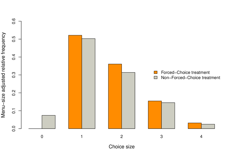
at menus of different sizes.

Alternatives chosen in the Non-Forced-Choice treatment (average response times, in seconds, in parenthesis) 0 1 2 3 4 Binary menus 11.95% (6.19) 74.52% (6.01) 13.53% (7.93) – – Ternary menus 6.85% (9.62) 44.67% (7.25) 43.33% (8.93) 5.15% (8.29) – Quaternary menus 3.70% (12.71) 33.53% (8.98) 33.28% (9.93) 27.02% (11.24) 2.47% (12.92) Alternatives chosen in the Forced-Choice treatment (average response times, in seconds, in parenthesis) 0 1 2 3 4 Binary menus – 83.77% (5.82) 16.23% (7.56) – – Ternary menus – 46.19% (7.31) 47.25% (8.44) 6.56% (8.88) – Quaternary menus – 28.50% (8.27) 41.01% (10.06) 27.29% (11.25) 3.18% (13.13)

Table 3 elaborates further on this theme by also showing how the relative frequencies of different choice sizes vary with the number of alternatives at different menus, and by also presenting the corresponding average response times. These conditional relative frequencies are uniformly higher in the Forced-Choice treatment for choice sizes 1 and 2 in binary and ternary menus. In addition, proportionally more subjects in that treatment chose 2, 3 or 4 gift-card pairs in quaternary menus too. As far as deferrals in the Non-Forced-Choice treatment are concerned, these were more likely in binary menus ($\approx$ 12%) than in ternary ($\approx$ 7%) or quaternary menus ($\approx$ 4%).

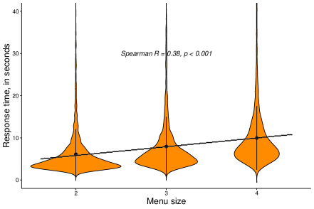
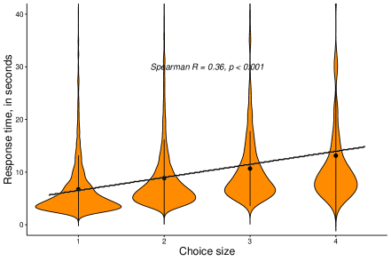
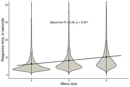
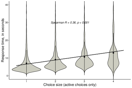
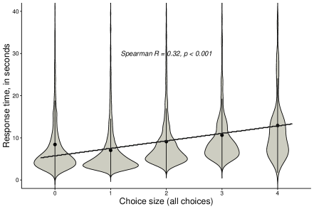
Notably, the average response time in both treatments was always lowest ($\approx$ 6 secs) when subjects chose a single pair of gift cards, while it increased monotonically (and statistically significantly) in similar ways as the size of choices and menus increased (Figure 2). These facts might be seen as intuitive evidence suggesting that the subjects’ decision was easier at menus where they chose a single gift-card pair, perhaps because that was their clearly preferred one. However, they are also consistent with an alternative interpretation whereby the time was shorter in those cases because subjects only had to move the mouse cursor on their computer to check a single choice box on their screen, thereby mechanically resulting in a shorter response time than when multiple items were selected from relatively larger menus. This argument is less relevant in the case of deferral decisions, however, where the average response time increases monotonically from (approximately) 6 to 10 to 13 secs when the menu includes 2, 3 and 4 alternatives, respectively. This suggests that the decision to defer was not generally based on some menu-irrelevant strategy (e.g. to reach the end of the experiment quickly), but was influenced instead by the relevant menu’s composition and, presumably, the subjects’ preferences at that menu. Finally, there is no significant difference in the distributions of response times in the subjects’ active choices across treatments ($p=0.612$; two-sided Mann-Whitney $U$ test).

Figure 2: Response times are positively correlated with menu and choice size in both treatments.

(a) Forced-Choice treatment

(b) Non-Forced-Choice treatment

Note: The violin plots are thicker (thinner) in regions with more (fewer) observations, and also show the conditional average response times and 95% confidence intervals per menu/choice size.

Figure 3: Distributions of the average choice proportions and menus where subjects chose everything or deferred.

(a) Forced-Choice treatment

(b) Non-Forced-Choice treatment

Notes: Unless otherwise noted, all $p$-values below are from two-sided Mann-Whitney $U$ tests. The distribution of average choice proportions (top panel) is significantly different between treatments, both when deferrals are included ($p=0.006$) and when they are not ($p<0.001$; figure not shown). The per subject distribution of menus where everything was chosen (middle panel) is not significantly different between treatments ($p=0.127$), although the rate at which subjects exhibited such behaviour is higher in the Forced-Choice treatment (8.4% vs 6.9%; $p<0.001$; two-sided Fisher’s exact test), and so is the proportion of subjects who did so at least once (71% vs 60%; $p=0.057$; two-sided Fisher’s exact test). See also main text. In the Non-Forced-Choice treatment the distribution of the number of menus where everything was chosen is not significantly different from the corresponding distribution where subjects deferred (bottom right panel; $p=0.498$).

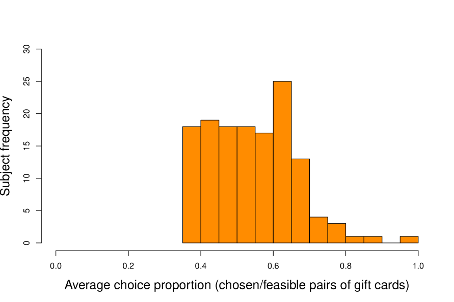
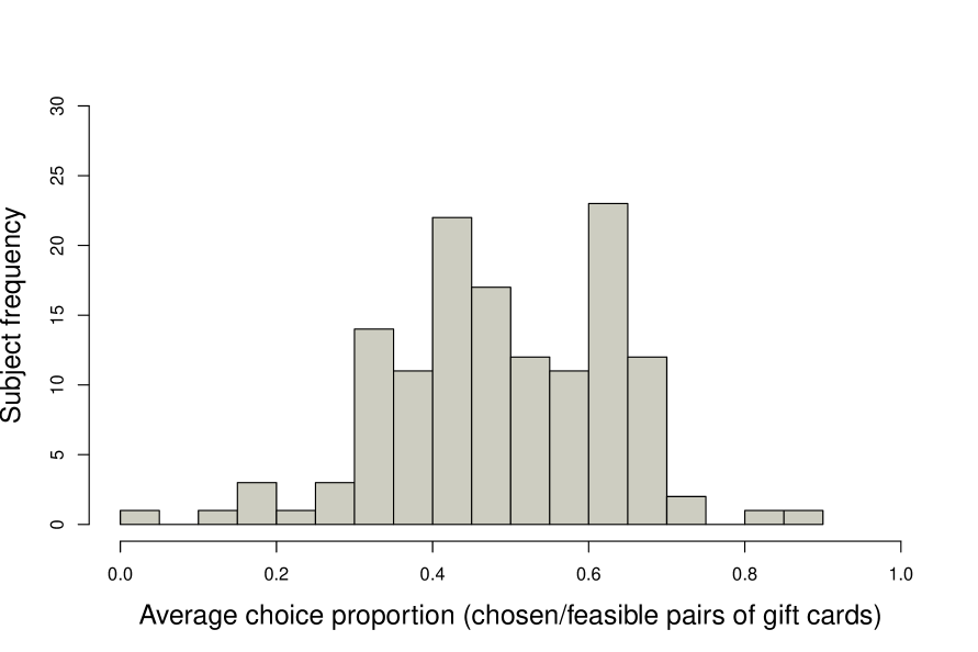
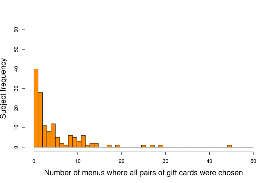
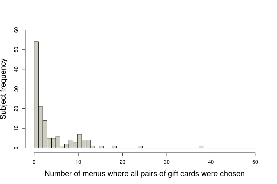
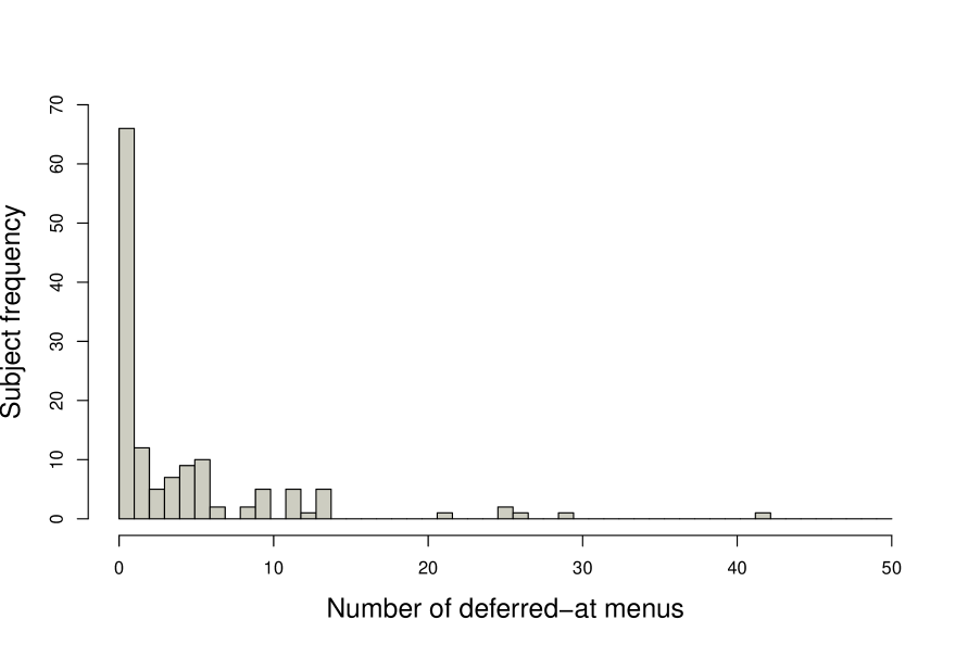
Next, we define a subject’s choice proportion at a menu as the number of chosen alternatives divided by the number of feasible alternatives at that menu. The distributions of average choice proportions across the two treatments are shown in Figure 3 (top panel) and are significantly different (higher in the Forced-Choice treatment) both when deferrals are included and when they are not ($p=0.006$ and $p<0.001$, respectively; two-sided Mann-Whitney $U$ tests). The mean/median choice proportions across all subjects in the Forced- and Non-Forced-Choice treatments were 0.54/0.5 and 0.49/0.5, respectively. That is, subjects in both treatments tended to choose around half of the feasible alternatives, on average.

Additionally, 69 subjects (51.1%) in the Non-Forced-Choice treatment deferred at least once, with deferrals per subject ranging between 1 and 42 (Figure 3-(b); bottom panel), and with a mean/median occurrence of 7.28/5 menus. Moreover, 81 subjects in this treatment (60%) chose all feasible gift-card pairs at least once, with such occurrences per subject ranging between 1 and 38 menus (Figure 3-(b); middle panel), and with a mean/median occurrence of 3.42/1 menus. By contrast, in the Forced-Choice treatment there were 98 subjects (71%) who chose everything at least once, with occurrences per subject ranging between 1 and 45 (Figure 3-(a); middle panel), and with a mean/median of 4.22/2 menus. The difference in the two proportions is borderline (in)significant at the 5% level ($p=0.058$; two-sided Fisher’s exact test). These findings lend further support to the possibility that, unable to delay their choice when faced with a hard decision, subjects are more likely to choose everything.

3.2         Choice Consistency

Following Costa-Gomes et al. (2022), for this analysis (which is summarized in Table 4) we first compare the proportions of subjects who made perfectly consistent active choices in the two treatments while also accounting here for possibly non-trivial indifferences. That is, we find the proportions of subjects whose single- and/or multi-valued choices –ignoring any deferral decisions– that are compatible with indifference-permitting utility maximization (see Section 4 for a formal statement of this model). These are approximately 4% and 13% for Forced- and Non-Forced-Choice subjects, respectively, and the difference is significant ($p=0.007$; two-sided Fisher’s exact test). Second, we compute the original Houtman-Maks (1985) index for each subject’s active choices and compare the two treatments’ distributions. Recall that this index gives the smallest number of active choices that need to be removed from a subject’s dataset in order for the remaining ones to be compatible with the model of rational choice. Forced- and Non-Forced-Choice subjects had a mean/median Houtman-Maks index of 10.81/10.5 and 9.05/6, respectively, and the two distributions are significantly different ($p=0.033$; two-sided Mann-Whitney $U$ test).

Table 4: Active-choice consistency in the two treatments.

Proportion of Average (median) number perfectly consistent of active choices away subjects from utility maximization Forced-Choice treatment ($N=138$)  3.62% (5/138)   10.81 (10.5) Non-Forced-Choice treatment ($N=135$)  12.59% (17/135)   9.05 (6.0) $p$-value 0.007 0.033

Note: The first and second $p$-values are from two-sided Fisher’s exact and Mann-Whitney $U$ tests, respectively.

Figure 4: Choice consistency is negatively correlated with average response times in both treatments.

(a) Forced-Choice treatment

(b) Non-Forced-Choice treatment

Notes: $R$ is the Spearman correlation coefficient and $p$ is the $p$-value. Shaded areas indicate 95% confidence intervals. There is no significant difference in the average response times between treatments ($p=0.550$; two-sided Mann-Whitney $U$ test).

Finally, to account for the fact that deferring at a menu can never decrease a decision maker’s active-choice consistency we also carry out subject-specific simulations to find how likely it would be for a possibly deferring subject to attain their Houtman-Maks score given that they made their active choices only at those particular menus where they did so. More specifically, in line with Selten (1991), Beatty and Crawford (2011) and Costa-Gomes et al. (2022), we compute in each treatment the Selten measure of predictive success of utility maximization on subjects’ active choices. We do so as follows: (i) for every experimental subject we create 10,000 datasets from as many artificial subjects who were restricted to make uniform-random active choices only at those menus where the experimental subject did so; (ii) we find the proportion of such subject-specific simulated datasets within this block that have a zero Houtman-Maks score when both indifference-permitting and indifference-excluding utility maximization are accounted for. Then, from the proportion, $p_{i}$, of perfectly consistent human subjects in treatment $i$ we subtract the average –over all such blocks– proportion of artificial subjects who are also perfectly consistent, $a_{i}$.

The closer the difference $m_{i}:=p_{i}-a_{i}$ is to 1, the higher the proportion of subjects who behaved as if they were utility maximizers, and the more likely it is that this could not have happened randomly. Low but positive values on the other hand could arise either because (i) relatively many experimental subjects were consistent but this could probably be due to chance; or (ii) because relatively few subjects were consistent and consistency in this environment was unlikely to occur by chance. It turns out that the latter case applies to the data from both our treatments, where we have $m_{FC}=p_{FC}-a_{FC}\approx 0.0362-0=0.0362$ and $m_{NFC}=p_{NFC}-a_{NFC}\approx 0.126-0=0.126$. Therefore, the results from these three analyses show that the negative forced-choice effect on consistency that was recently documented for single-valued choices in Costa-Gomes et al. (2022) extends to possibly multi-valued choices from twice as many menus (50 vs 26), over more alternatives (6 vs 5), and when indifference-permitting utility maximization is also accounted for.

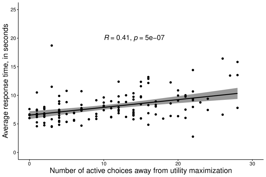
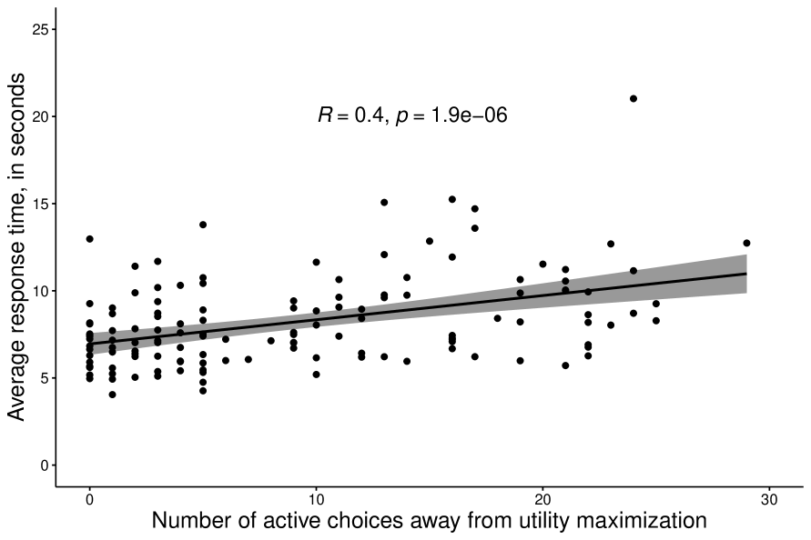
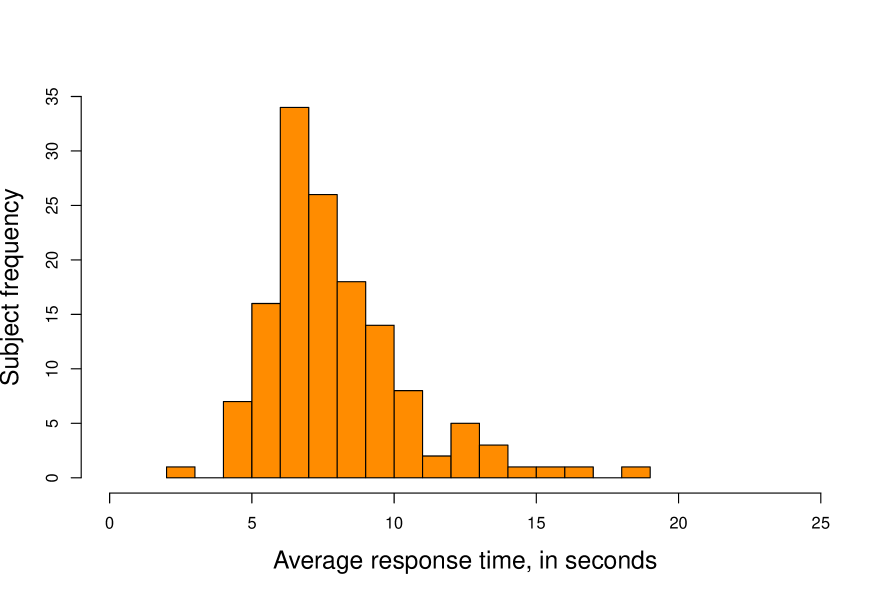
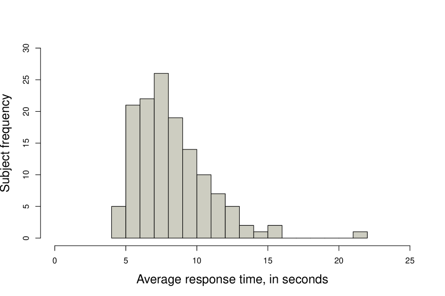
We also ask how a subject’s choice consistency, as captured by the above Houtman-Maks index, is related to their response times. Figure 4 (top panel) shows that there is a significant –and nearly identical, with an approximate coefficient $R=0.4$– positive correlation in each treatment between subjects’ active-choice Houtman-Maks indices and their average response times. That is, subjects’ choice consistency is negatively correlated with the time it takes for them to make their active choices. As we noted earlier, this interesting finding is broadly consistent with the important prediction of the drift-diffusion neuro-economic model whereby shorter response times are more likely when a clearly preferred alternative exists, which would imply in turn more consistent active-choices behaviour. Another possible explanation for this finding is that subjects with a higher cognitive ability (an unmeasured variable in this study) are both more consistent and faster than subjects with a lower cognitive ability. A distinct possible explanation is that spending more time before deciding is more characteristic of people who are prone to second thoughts and therefore more likely to be involved in choice reversals when presented with a series of decision problems. Conversely, it is also possible that subjects who had neither a stable preference relation over the choice alternatives nor a clear decision rule ended up spending more time on average at each menu, but without this extra time ultimately alleviating the effects of their ambivalence.

Figure 5: Choice consistency is negatively correlated with the average choice size.

(a) Forced-Choice treatment

(b) Non-Forced-Choice treatment

Note: $R$ is the Spearman correlation coefficient and $p$ is the $p$-value. Shaded areas indicate 95% confidence intervals.

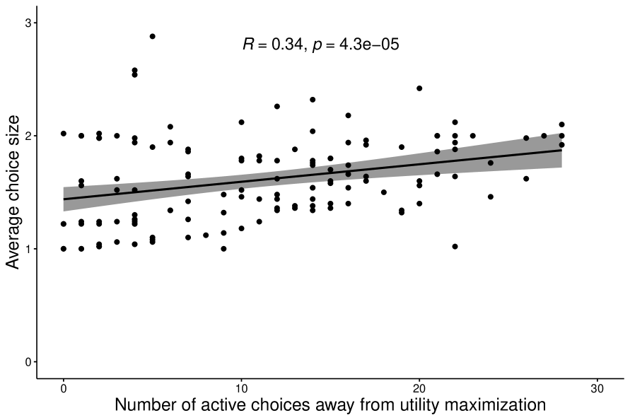
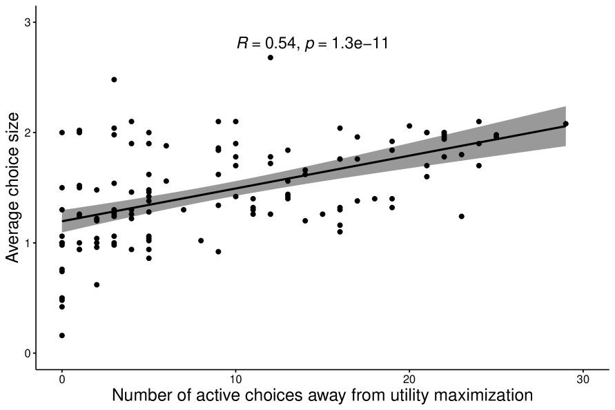
Figure 5 further shows that there is also a significant negative correlation between subjects’ active-choice consistency and their average choice sizes in each of the two treatments, with this relationship being more pronounced for Non-Forced-Choice subjects ($R=0.54$ vs $R=0.34$ on Houtman-Maks index). In line with our preceding findings and discussion, an intuitive explanation for this difference is that, unlike Non-Forced-Choice subjects, their Forced-Choice counterparts could not defer at menus where they might perhaps have wished to do so, opting instead for more
alternatives per menu. But while delaying choice when confronted with a difficult problem safeguards
the consistency of one’s behaviour, choosing more (possibly all) alternatives could do the opposite because it opens up more possibilities for choice reversals/cycles to emerge.

Figure 6: Subjects who deferred are significantly more consistent in the Non-Forced-Choice treatment.

Some additional support to this explanation, finally, is obtained by also comparing the active-choice consistency of Non-Forced-Choice subjects who deferred at least once to the consistency of those who did not. More specifically, 14 of the 69 (20%) deferring subjects were perfectly consistent in this sense, while 3 of the 66 (4.5%) non-deferring ones were such (equivalently, 14 out of the 17 perfectly consistent in this treatment deferred at least once). The difference between these two proportions is significant ($p=0.008$; two-sided Fisher’s exact test). Moreover,
the two groups had an average Houtman-Maks score of 6.83 and 11.38, respectively, and the difference in the two distributions is significant as well ($p=0.001$; two-sided Mann-Whitney $U$ test). In fact, as shown in Figure 6,
deferring subjects are uniformly more consistent than non-deferring ones in the sense that the distribution of their Houtman-Maks scores first-order stochastically dominates the corresponding distribution of the latter subjects. That is, for every number less than or equal to $n$, and for every $n$, non-deferring subjects were more likely to be strictly more than $n$ active choices away from utility maximization. This within-treatment effect is in the spirit of the negative forced-choice effects that were first reported in Costa-Gomes et al. (2022) and also above, and clarifies the important mediating role of deferrals for consistency, even in cases such as this where the average/median number of deferrals is 7.3/5 out of 50 and where decision makers are allowed to also make multi-valued choices.

4         Individual-Level Analysis

4.1         Three Deterministic Models of Preference-Maximizing Choice

As was mentioned in the Introduction, in the main part of our individual-level analysis we consider three simple choice models of deterministic preference maximization that impose a rich structure on observable behaviour:

1. Rational choice/utility maximization.

2. Undominated choice with incomplete preferences.

3. Dominant choice with incomplete preferences.

We focus on these models for several reasons. First, they all feature stable preferences and predict both single-valued and multi-valued choices under different preference orderings, with multi-valuedness potentially interpretable as revealing indifferences and single-valuedness as revealing strict preferences. Second, they impose strong behavioural restrictions. In particular, all three models satisfy the fundamental Property $\alpha$ (Sen, 1971) or Contraction Consistency principle, which requires an alternative to be chosen at a menu whenever it is feasible at that menu and also chosen at a larger menu. In addition, the first and third models predict active choices that are actually consistent with the Congruence/Strong Axiom of Revealed Preference principle, which rules out all forms of choice cycles. Third, these models are defined in terms of (and hence in principle allow the analyst to recover) a single preference relation, thereby making the welfare-relevant parts of the analysis unambiguous. Fourth, all three models are uniquely identifiable. That is, if a decision maker’s observable behaviour is perfectly compatible with one of these models and the available data are sufficiently rich (as is the case in our experiment), then there is a unique preference relation with which that model explains the individual’s behaviour. Fifth, they are sufficiently computationally tractable to allow for the behaviourally intuitive optimization-based goodness-of-fit test that we describe below. Finally, in light also of the preceding discussion about the structure and possible interpretation of the experimental design, and in light also of the empirical findings presented above, the three models predict the kinds of active-choice and deferring behaviour that one might expect to observe in our data.

To state the models formally we first define a decision maker’s choice dataset $\mathcal{D}=\big{(}A_{i},C(A_{i})\bigr{)}_{i=1}^{k}$ on a finite grand choice set $X$ to be a collection of pairs that comprise a non-empty menu $A_{i}\subseteq X$ and a -possibly empty- set of alternatives that were chosen at this menu when the decision maker was presented with it. Thus, $\emptyset\subseteq C(A_{i})\subseteq A_{i}$ holds for all $i\leq k$. Dataset $\mathcal{D}$ is explainable by rational choice/utility maximization if there exists a complete and transitive preference relation $\succsim$ on $X$ such that, for all $i\leq k$,

$$C(A_{i})=\{x\in A_{i}:x\succsim y\text{ for all }y\in A_{i}\}.$$ (1)

If, instead, (1) is true for all $i\leq k$ with respect to a reflexive and transitive but incomplete preference relation, then $\mathcal{D}$ is explainable by the model of (maximally) dominant choice with incomplete preferences. In that case we have

$$C(A)\neq\emptyset \Longleftrightarrow \text{ there is }x\in A\text{ such that }x\succsim y\text{ for all }y\in A,$$

$$C(A)=\emptyset \Longleftrightarrow \text{ for all }x\in A\text{ there is }y\in A\text{ such that }x\not\succsim y.$$

Finally, $\mathcal{D}$ is explainable by the model of undominated choice with incomplete preferences if there is a reflexive, transitive and incomplete preference relation $\succsim$ whose asymmetric part is $\succ$, such that, for all $i\leq k$,

$$C(A_{i})=\{x\in A_{i}:y\not\succ x\text{ for all }y\in A_{i}\}.$$ (2)

The model of rational choice/utility maximization was characterized by Richter (1966) in a general environment that encompasses the one within which we are operating here. The model of undominated choice with incomplete preferences was introduced by Schmeidler (1969) in a general equilibrium setting and was analyzed choice-theoretically under a variety of decision environments and preference structures by, most notably, Schwartz (1976), Bossert et al. (2005), Eliaz and Ok (2006), Bossert and Suzumura (2010) and Stoye (2015). Dominant choice with incomplete preferences was studied theoretically in Gerasimou (2018a) and empirically in Costa-Gomes et al. (2022), with the latter analysis limited to an environment of single-valued non-forced choice experimental data which, in particular, do not allow for testing the model of undominated choice or distinguishing between indifference and indecisiveness in either of the two models of choice with incomplete preferences.

The two models of incomplete-preference maximization are logically distinct. Moreover, if we replace the term “incomplete” with “possibly incomplete” in their respective statements, then these models generalize rational choice in different ways. The first does so by relaxing active-choice consistency while retaining the decisiveness (non-emptiness) assumption that requires $C(A_{i})\neq\emptyset$ for all $i\leq k$. The second model does so by relaxing the decisiveness assumption while retaining active-choice consistency.

We test our possibly multi- and/or empty-valued experimental choice data for compatibility with each of these three models. We do so by using a model-based extension of the classic Houtman and Maks (1985) (HM) method that is routinely used in the empirical revealed preference analysis of single-valued consumer-demand data. Specifically, we ask what is the smallest number of decisions that need to be dropped/changed in a subject’s dataset in order for it to be compatible with that model under some of its instances/admissible preference orderings. We refer to this number as the model’s distance score. These scores were computed using a method that was originally introduced in Costa-Gomes et al. (2016, 2022) and since (Gerasimou and Tejiščák, 2018) has been extended considerably and made freely available online in the open-source desktop application  . These scores were computed by applying the method that was originally introduced in Costa-Gomes et al. (2016) (a working-paper version of the study published in 2022) and is now greatly extended and freely available online in the open-source desktop application  (Gerasimou and Tejiščák, 2018).

More specifically, a brute-force algorithm was implemented for these computations. This involved the production of all choice datasets that are generated by all possible instances of every model, and comparing each such dataset against every subject’s own dataset in order to find the model(s) and instance(s) that are closest to it in the minimum distance-score sense. Therefore, this method detects perfect as well as approximate model fits, and in the latter case it quantifies the approximation in an intuitive way that may be interpreted as the number of “mistakes” made by an agent who might be portrayed as following a particular decision rule. For other approximations that have been proposed and/or used recently for distinct classes of models and choice environments we refer the reader to Choi et al. (2007); Echenique et al. (2011); Choi et al. (2014); Apesteguia and Ballester (2015); Dean and Martin (2016); Dembo et al. (2021); Fudenberg et al. (2023); Cherchye et al. (2023); Echenique et al. (2023) and references therein.

We stress that despite the vast numbers of weak orders (4,683), partial orders (130,023) and, especially, incomplete preorders (209,527) that are defined on a set of 6 alternatives (OEIS, 2021), the above tool makes such an exact computation possible very quickly –in less than 12 seconds– for all subjects in each treatment, for each of the three models. We also stress that, although this tool lies within the rapidly expanding realm of artificial-intelligence technologies, broadly interpreted, it builds on combinatorial-optimization methods to arrive at exact solutions to a clearly defined and behaviourally intuitive problem. In particular, it does not feature so-called “deep-learning” decision algorithms that build on neural-network structures which may be unclear/uninterpretable or prone to over-fitting. Finally, although the brute-force algorithm is linear in the number of subjects but exponential in the number of alternatives, the model-rich distance-score method itself is scalable and can be extended to analyse datasets that are derived from much larger sets of alternatives by employing powerful open-source constraint solvers such as Gecode (Gecode Team, 2006) and Z3 (Moura and Bjørner, 2008, Microsoft Research).

Table 5: Classification of subjects who are perfectly or approximately explainable by one of the three models.

Undominated Dominant Rational Choice with Choice with Choice Incomplete Incomplete All Preferences Preferences Forced-Choice treatment ($N=138$) % of subjects with score $=$ 0 3.62% 0% 0% 3.62% % of subjects with score $\leq$ 5 33.33% 2.17% 0% 35.50% % of subjects with score $\leq$ 10 46.38% 8.70% 0% 55.07% Mean/median best score ($\leq 10$) 4.06/4 7.25/8 – 4.56/4 Minimum score in simulations 25 23 – 23 Mean/median best-model 1.17/1 1.00/1 – 1.15/1 preference orderings (score $\leq 10$) Non-Forced-Choice treatment ($N=135$) % of subjects with score $=$ 0 2.22% 0% 5.19% 7.41% % of subjects with score $\leq$ 5 18.51% 2.96% 21.48% 42.96% % of subjects with score $\leq 10$ 24.44% 5.19% 28.15% 57.78% Mean/median best score ($\leq 10$) 4.15/3 5.57/5 3.39/3 3.91/3 Minimum score in simulations 27 26 18 18 Mean/median best-model 1.00/1 1.29/1 1.08/1 1.06/1 preference orderings (score $\leq 10$)

Notes: Model-score ties were always broken in favour of Rational Choice/Utility Maximization (no other ties emerged). When Rational Choice/Utility Maximization was not a subject’s optimal model, the difference between this and the optimal model’s score was on average 4.2 and 6.5 in the Forced- and Non-Forced-Choice treatments, respectively. Finally, in the analysis of Non-Forced-Choice data we also included a deferral-permissive variant of Undominated Choice with Incomplete Preferences whereby decisions are made as in the original version of that model except that the decision maker is assumed to defer whenever no strict preference comparisons exist between any two feasible alternatives. Including this model did not change the results but produced 8 ties between this hybrid variant and the model of Dominant Choice with Incomplete Preferences.

Figure 7: Perfect and approximate fits for the models of rational choice, undominated and dominant choice with incomplete preferences, and the corresponding fits from simulated subjects.

(a) Forced-Choice treatment

(b) Non-Forced-Choice treatment

Notes: (i) For experimental subjects the histograms show the relative frequencies of those who are best-explained by the respective models and have a distance score between 0 and 10; (ii) ties between Rational Choice and each of the other two models were broken in favour of the former: 92 such ties occurred between Rational and Undominated Choice (60 and 32 ties under Forced and Non-Forced Choice) and 39 between Rational and Dominant Choice (Non-Forced Choice); there were no ties between the two incomplete-preference models.

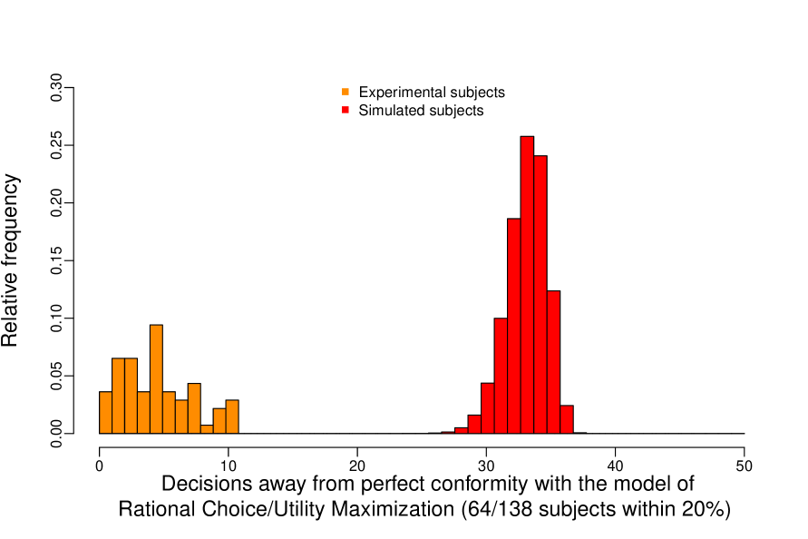
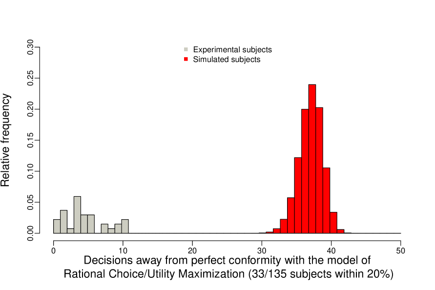
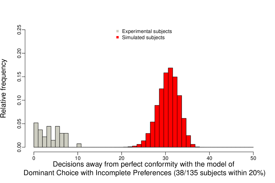
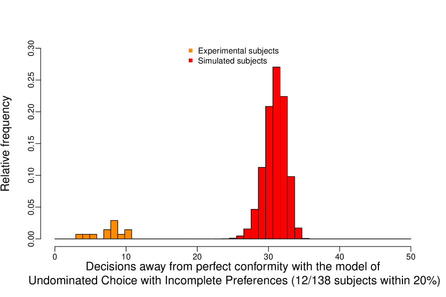
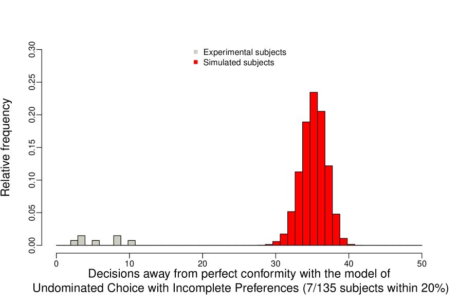
Table 5 and Figure 7 present summaries of this goodness-of-fit analysis for both the Forced- and Non-Forced-Choice subjects. In line with standard practices in revealed preference analysis whereby one also wishes to understand the extent to which a certain behaviour or perfect/approximate model fit could have been generated randomly (Bronars, 1987), we also performed our model analysis on 100,000 simulated datasets of artificial uniform-random behaving subjects under both a forced- and a non-forced choice configuration (details on the simulations’ structure are available in Appendix C). The distance-score distributions of simulated subjects are juxtaposed in the relevant graphs of Figure 7 to those of the experimental subjects that are perfectly/approximately explained by one of the three models, while the minima of the simulated-subject distributions are also presented in Table 5.

For experimental subjects, rational choice often tied with one but never both of the other two models; our classification broke ties in favour of that model whenever a subject’s distance score was produced by rational choice and another model (see the notes of Table 5 for more details). Under this tie-breaking assumption, and in line also with model-approximation methods used in the above-cited studies, our two exhibits show the number, proportion and relative-frequency distributions of distinct subjects that are on average within 10% or 20% (equivalently, within 5 or 10 decisions) away from being explainable perfectly by an instance of some model, separately for each of the two experimental treatments. We chose this conservative approximation range for two factors: (i) simulations suggest that a distance score of 10 for any of the three models is extremely unlikely to occur randomly in this decision environment (see Table 5 and 7); (ii) for subjects with a distance score up to 10 there is typically only one best-matching preference ordering that explains their behaviour under the respective subject-optimal model.

The total number (percentage) of Non-Forced-Choice subjects with a perfect, 10%- or 20%-approximate fit was 10 (7.4%), 58 (43%) and 78 (58%), respectively. Thirty-three, 7 and 38 subjects in the latter group were categorized under rational choice, undominated and dominant choice with incomplete preferences, respectively, while 3 and 7 were perfectly compatible with the first and third of these models. The total number of Forced-Choice subjects with a perfect, 10% or 20%-approximate fit was 5 (3.6%; all under rational choice), 49 (35.5%) and 76 (55%), respectively, with 64 and 12 of those in the latter group classified under rational choice and undominated choice with incomplete preferences. This model fit was slightly better on average in the Non-Forced-Choice treatment than in the Forced-Choice one (mean/median scores: 3.91/3 vs 4.56/4), although the distributions were not significantly different ($p=0.173$; two-sided Mann-Whitney $U$ test). Similarly, and consistent with the results from the previous section, the proportion of subjects who were best-matched by one of the two models of consistent active decision making is higher in the Non-Forced-Choice treatment (40% vs 33.3% and 52.6% vs 46.4% under the 5- and 10-decisions approximation thresholds, respectively), while the proportion of subjects best-matched by the third model is lower in that treatment (5% vs 9%). Moreover, when rational choice was not the best-matching model, its distance score was on average 6.5 and 4.2 units higher in these treatments, respectively. Finally, the highest distance score of 10 in these experimental subjects is far below the corresponding minimum scores of simulated random-behaving subjects, which ranged between 18 and 27.

As far as preference recovery is concerned, for the vast majority of these subjects there was a unique preference ordering that generated their distance score under their best-matching model, with the mean/median number of such orderings being 1.15/1 and 1.06/1 in the Forced- and Non-Forced-Choice treatments, respectively. The directed graphs of the subject-optimal preference orderings that were recovered by this method are shown in Appendix D for all 154 subjects that were included in this analysis. Importantly, for 110 (71%) of them the recovered optimal preference relation(s) has a non-trivial indifference component. This highlights the potential usefulness of eliciting indifferences for revealed preference and welfare analysis.

Figure 8: Thirty-seven of the 38 subjects that were best-matched by dominant choice with incomplete preferences were unlikely to have achieved this classification at random given the menus where they deferred.

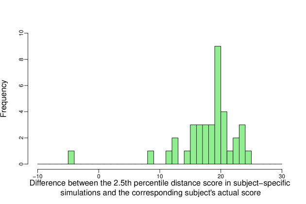
Prompted by the greater permissiveness of behaviour in the Non-Forced-Choice treatment, for the 38 subjects who are best-explained by the dominant-choice model we also conducted a new robustness check. By analogy to the way in which the predictive success of rational choice on non-forced-choice subjects’ active-choice consistency was evaluated in Section 3.2, we created 10,000 simulated subjects for each of the 38 human participants who were best-matched by that model, holding fixed in each simulations block the menus at which the relevant human participant deferred. This allows for evaluating the predictive success of the dominant-choice model’s 20%-approximation range in this decision environment. Figure 8 shows the histogram with distance-score differences (for this model) between the 2.5th percentile value in each subject-specific simulations block and the relevant subject’s actual distance score. For 37 of these subjects (97%) the difference is positive and typically much greater than 10 score units. The one subject for whom this isn’t the case deferred at 42 of the 50 menus (cf Figure 3(b)-bottom panel) and has distance score 7. This analysis suggests that the dominant-choice model is not excessively permissive in this environment, and that its good fit is useful in explaining behaviour and eliciting preferences.

4.2         Distinguishing Between Indifference and Indecisiveness

For a decision maker with incomplete preferences who is also indifferent between some alternatives, a non-trivial question that emerges naturally is how one might use observable behavioural data in conjunction with some model in order to separate those pairs of alternatives between which the agent is indifferent from those where the agent is indecisive/unable to compare. Eliaz and Ok (2006) were the first to raise and provide an answer to this question. Taking the model of undominated choice as their primitive, the authors focused on and characterized the special case where the model’s rationalizing incomplete preference relation $\succsim$ is “regular” in the sense that whenever $x\not\succsim y$ and $y\not\succsim x$ are both true, then there is $z\in X$ such that either $x\not\succsim z$, $z\not\succsim x$ and $y\succ z$ or $z\succ y$, or $y\not\succsim z$, $z\not\succsim y$ and $x\succ z$ or $z\succ x$ (Table 6 shows how the number of indifference-permitting regular incomplete preorders varies when $|X|\in\{3,4,5,6,7\}$). The authors’ proposed distinction can then be summarized as follows:

An agent whose incomplete preferences are captured by a regular preorder and
who maximizes these preferences according to the undominated-choice model
is revealed to be:

indifferent between $x$ and $y$ only if $\big{[}$$x,y\in A$, $y\in C(A)$$\bigr{]}$ $\Rightarrow$ $x\in C(A)$;

indecisive between $x$ and $y$ only if $x\in C(A)$, $y\in A\setminus C(A)$, $y\in C(B)$, $x\in B$
                                                         for distinct menus $A$ and $B$.

In words, the agent is indifferent only if the two options are either chosen or rejected together when both are feasible, while they are indecisive only if one is chosen over the other in some menu and the latter is chosen in the presence of the former in another menu. Importantly, the revealed indifference relation here is transitive, whereas the revealed indecisiveness one is not (see also Mandler, 2009). Also importantly, although this choice-reversal-based distinction between the two notions is intuitive, it is not robust. Indeed, any behaviour that is compatible with such an indifference-permitting instance of that model is observationally equivalent to the same instance of the model where the decision maker is simply indecisive between any two alternatives that are not ranked by strict preference (see also Theorem 1 in Bossert et al., 2005 and Theorem 3.3 in Bossert and Suzumura, 2010).

Table 6: Enumeration of regular incomplete preorders that allow for non-trivial indifferences.

All Regular $|X|$ indifference-permitting indifference-permitting % incomplete preorders incomplete preorders 3 3 0 0.00% 4 85 54 63.53% 5 2,290 1,705 74.45% 6 75,541 60,455 80.03% 7 3,363,129 2,799,615 83.24%

Source: Output from constraint-satisfaction problems written in the Essence^′ language and solved by the MINION solver (Gent et al., 2006) using the Savile Row modelling assistant (https://savilerow.cs.st-andrews.ac.uk/).

Gerasimou (2018a) recently noted a distinct and robust behavioural separation between indifference and indecisiveness is afforded by the dominant choice model. This can be summarized as follows:

A decision maker whose incomplete preferences are captured by a preorder and
who maximizes these preferences according to the dominant-choice model
is revealed to be:

indifferent between $x$ and $y$ if and only if $\big{[}$$x,y\in A$, $y\in C(A)$$\bigr{]}$ $\Rightarrow$ $x\in C(A)$;

indecisive between $x$ and $y$ if and only if $x,y\in A$ $\Rightarrow$ $x,y\not\in C(A)$.

In words, the agent is indifferent iff both options are either chosen or rejected together when both are feasible, and they are indecisive between these options iff neither is ever chosen in the presence of the other. This distinction is obviously robust because reducing a relation’s indifferences to incomparabilities in this case generates different active-choice and deferring behaviour. Notably, moreover, it turns out that the generally intransitive revealed indecisiveness relation that is derived from this model coincides with the incomparability relation that is derived from the strict welfare preference relation that was studied in Bernheim and Rangel (2009), which these authors motivated as possibly applicable in model-free environments of forced choice.

Figure 9: A subject’s complete preferences, optimally recovered with the model of utility maximization.

Notes: Perfect fit. Arrows point to inferior alternatives/indifference classes.

Figure 10: A subject’s incomplete preferences, optimally recovered with the undominated-choice model.

Notes: Approximate fit (distance score: 5). Arrows point to inferior alternatives/indifference classes. The left (right) graph depicts the strict- (weak-)preference interpretation of the subject’s choices. In the right graph the subject is revealed indifferent between alternatives $A$ and $F$ and revealed indecisive between e.g. $A$ and $D$. For example, $C(\{A,F\})=C(\{A,F,D\})=\{A,F\}$ while $C(\{A,D\})=\{A,D\}$ and $C(\{A,C,D,E\})=\{D,E\}$. In the left graph they are revealed indecisive between $A$ and $F$ too.

Figure 11: A subject’s incomplete preferences, optimally recovered with the dominant-choice model.

Notes: Perfect fit. Arrows point to inferior alternatives/indifference classes. The subject is revealed indifferent between $B$, $D$, $E$ and revealed indecisive $A$, $F$, $C$. For example, $C(\{B,D\})=\{B,D\}$, $C(\{D,E\})=\{D,E\}$, $C(\{B,E\})=\{B,E\}$, $C(\{B,D,E\})=\{B,D,E\}$, while $C(\{C,F\})=C(\{F,A\})=C(\{C,A\})=C(\{C,F,A\})=\emptyset$.

The multi- and/or empty-valued experimental choice data and the non-parametric optimization goodness-of-fit method that were presented in the previous (sub)sections jointly allow us to test for the potential presence of both these theory-guided distinctions for the first time. Additionally, going beyond the boundaries of the above two theoretical studies which assumed that the analyst observes active choices/deferrals at all menus that can be derived from the grand choice set, this method allows us to carry out this test and recover the individual’s strict preferences and, where relevant, indifferences and incomparabilities from an incomplete collection of menus.

We find that a total of 6 subjects (5 in the Forced-Choice treatment) out of the 19 who were best-matched by the undominated-choice model revealed “regular” incomplete preferences that afford the Eliaz-Ok distinction between indifference and indecisiveness (range of distance scores: [5,10]). Figure 10 illustrates one such example, with the graph on the right depicting the revealed incomplete weak preference relation and the graph on the left the observationally equivalent revealed incomplete strict preference relation.

We also find that 30 out of the total 38 Non-Forced-Choice subjects for whom the dominant-choice model provided the best fit (including the 5 subjects for whom this fit was perfect) revealed incomplete preferences with a non-degenerate indifference part (range of distance scores: [0,10]). Figure 11 depicts such an example.

Although indifference is generically non-existent for a large class of incomplete preference relations that are defined on a space of bundles of continuous commodities or uncertain acts (Gerasimou, 2018b), this is not so when such preferences are over finitely many indivisible goods, as in the choice environment we consider here. Indeed, the preceding analysis suggests that out of all 57 subjects that the two models of incomplete-preference maximization explain optimally in our sample, 36 (63%) exhibited behaviour that allows for recovering a transitive strict preference relation together with a transitive indifference relation and a generally intransitive incomparability/indecisiveness relation.

4.3         Satisficing

Simon (1956) famously coined the term satisficing to describe resource-constrained agents who, instead of searching through all available alternatives in order to find the best, only search until they find one that meets an acceptability threshold. Two recent forced-choice studies that tested the satisficing hypothesis in economics are Reutskaja et al. (2011) and Caplin et al. (2011). The former found weak evidence for such behaviour in choice from lists of food snacks under intense time pressure, whereas the latter found strong evidence in choice from lists of monetary amounts that were described verbally through a series of additions and subtractions, without (or with limited) time pressure. The fact that all 50 menus in both treatments of our experiment were presented vertically as unnumbered lists allows us to add to this literature by complementing the preceding model-based analysis with a test for satisficing in the present time-unconstrained decision environment of multi-valued choice over pairs of gift cards.

To this end, we first conduct a relatively narrow but potentially informative test of satisficing by focusing on the frequency with which subjects opted to choose only the first alternative that appeared in the menus they saw, and then asking whether this frequency can be viewed as being above and beyond what might be reasonably interpretable differently. Specifically, we find that 5 and 4 subjects (3.3%) in the Forced- and Non-Forced-Choice treatments, respectively, who were not classified as approximately explainable by one of the three deterministic models discussed earlier chose only the first option at frequencies that strictly exceeded the 97.5% cut-off values of 0.28 and 0.29 that are derived from the relevant simulations. These numbers rise to 27 and 20 (17%), respectively, if the non-randomness criterion is retained but the model-classification requirement is dropped.

In addition, we compute and study the average position of each subject’s chosen item(s) in the 50 menus’ list orderings because, intuitively, an unusually low average value of this metric could also be indicative of satisficing behaviour for the subject in question. We find that for an additional 7 and 5 (4.4%) subjects in the Forced- and Non-Forced-Choice treatments, respectively, who were not classified as approximately explainable by one of the three deterministic models that were discussed above, the average positions of their chosen item(s) in the 50 menus’ list orderings were strictly below the 2.5% percentile cut-off value of 1.84 that is derived from simulated uniform-random forced choices. These two distinct analyses therefore suggest that a total of 21 subjects (7.7%) who were not model-classified in Table 5 might be thought of as exhibiting a systematic satisficing behaviour.

Figure 12: Forced-Choice subjects are more likely to select items that are higher up in the menu list.

(a) Forced-Choice treatment

Distribution range: $[1.15,2.25]$

(b) Non-Forced Choice treatment

Distribution range: $[1.74,2.32]$

Note: $p=0.009$; two-sided Mann-Whitney $U$ test.

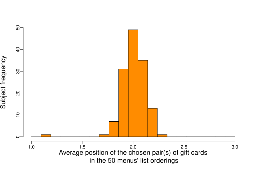
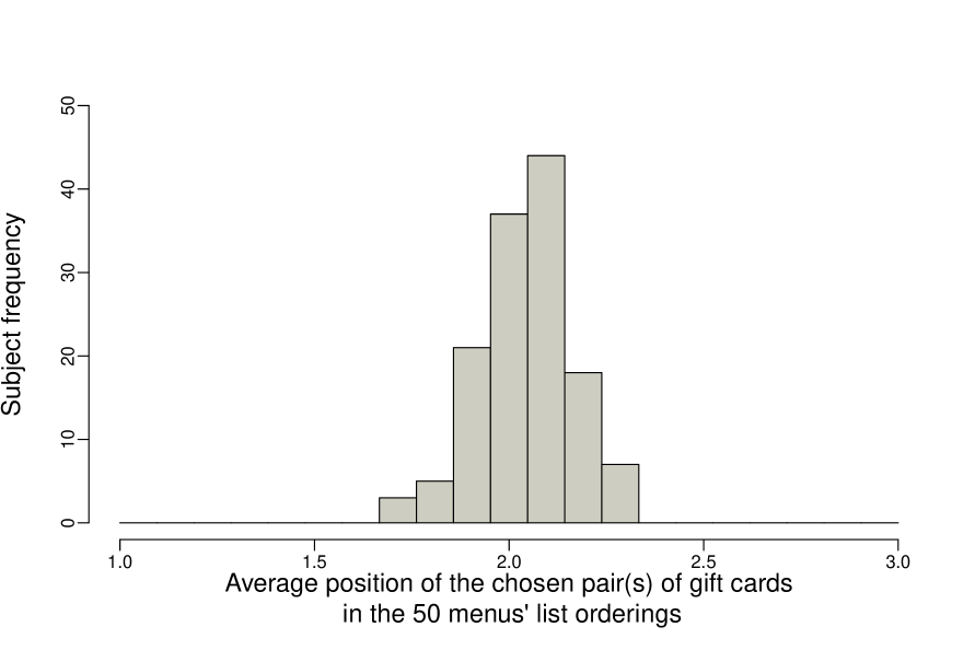
Interestingly, a cross-treatment comparison of how the average positions of all chosen alternatives are distributed (see Figure 12) indicates that Forced-Choice subjects may be significantly more likely to choose items that appear higher up in the menu list ($p=0.009$; two-sided Mann-Whitney $U$ test). This finding could be explained intuitively as follows: for individuals who are either insufficiently motivated to make 50 careful decisions over 2–4 pairs of gift cards in an experimental lab or find the task to be cognitively challenging, being unable to avoid/defer the decision at a small cost could make the use of a non-compensatory decision heuristic such as satisficing more likely.

4.4         Preference for Randomization

Agranov and Ortoleva (2017, 2023), Dwenger et al. (2018) and Agranov et al. (2022), among others, have recently documented a preference for randomization in repeated choices from binary menus of money lotteries. Such a preference refers to subjects’ frequent tendency to change their choices from one occurrence of a menu to the next, and their willingness to even incur a small cost in order to have their choice determined randomly. In addition to the indifference-permitting goodness-of-fit analysis of the three models that was presented earlier, the aspect of our experimental design whereby subjects are rewarded with a random alternative at a menu if they chose all alternatives at that menu allows us to test for the existence of a similar preference for randomization in our data, even without any choice repetitions. Being another by-product of the experiment’s features, however, this additional test is limited in its scope because the experimental design was not constructed to detect all possible manifestations of preference for randomization in multi-valued choice environments.

As with our analysis of satisficing, to proceed with this investigation we regard a subject as potentially exhibiting such a preference if: (i) they are not approximately explainable by one of the three deterministic models of preference maximization; and (ii) the number of menus were they chose everything strictly exceeds the 97.5% simulations-based cut-off values of 14 and 11 menus in the Forced- and Non-Forced-Choice treatments, respectively. Both criteria are satisfied by 3 and 4 subjects (2.5%) in the Forced- and Non-Forced-Choice treatment, respectively, with these numbers rising to 6 and 9 (5.5%) when the first criterion is dropped. In addition, none of these 7 subjects belongs to the “satisficing” category that was defined above. This finding adds to the existing and growing literature on preference for randomization by showing that such a preference could potentially manifest itself in binary as well as non-binary menus of riskless alternatives, even when the choice-deferral option is feasible and acts as another obvious way for an individual to deal with a difficult decision, and even in non-repeated-choice environments.

5         Concluding Remarks

This paper proposes and implements theory-guided methods of data collection and analysis that aim to contribute towards eliciting a decision maker’s possibly weak or incomplete preferences and, where relevant, towards distinguishing between their indifference and indecisiveness parts. On the data-collection side, the paper contributes an incentivized experimental design with multi-valued forced- and non-forced choice treatments. On the data-analytic side, it deploys a model-rich combinatorial-optimization method that allows for recovering an individual’s possibly weak or incomplete preferences from their multi-valued choices in a model-optimal way. This extends the celebrated Houtman and Maks (1985) approach to models of bounded rationality.

Despite the relatively large number of decisions made, the behaviour of 56% of all subjects in our experimental sample is either perfectly or approximately matched by some simple but richly structured deterministic model of complete or incomplete preference maximization, with uniquely recovered and indifference-exhibiting preferences in the vast majority of cases. Rational choice accounts for the behaviour of 63% of all subjects in this group (35.5% of the total), while the two models of incomplete-preference maximization together account for the remaining 37% (21% of the total). Consistent with our additional results which show that Forced-Choice subjects are significantly more inconsistent than Non-Forced-Choice ones, the model-based analysis further suggests that proportionately more subjects in the latter treatment are well-approximated by a model of consistent active choices, although this difference is not significant. Additionally, the optimal preference relation that is recovered conditional on a subject’s best-matching model typically features a non-trivial indifference relation, and therefore highlights the importance of accounting for indifferences in revealed-preference analyses. Finally, exploiting two relevant aspects of the experimental design allows for inferring that a further 10% of all analysed subjects could be thought of as engaging in systematic satisficing behaviour or displaying a robust preference for randomization. This increases to 66% the proportion of individuals whose behaviour can be categorized as following a specific pattern.

Our analysis points to the potential usefulness of multi-valued and indifference-permitting choice experiments. It also highlights the importance of methodologically pluralistic methods that allow for recovering preferences and/or choice rules by comparing observed behavioural with the predictions made by utility maximization as well as by models of bounded-rational preference maximization or decision heuristics.

Online Appendix to “Towards Eliciting Weak or Incomplete Preferences in the Lab: A Model-Rich Approach”

Appendix A Experiment Details

A.1          Instructions: Non-Forced-Choice Treament (verbatim)

A.2          Instructions: Forced-Choice Treament (verbatim)

A.3          The six pairs of £10 gift cards used in the experiment

A.4          Example decision problem shown in the main part*

* This example is taken from the Non-Forced-Choice treatment. Presentation in the Forced-Choice treatment is identical except that “I’m not choosing now” is unavailable and the instruction reads “Please choose one of more gift cards from this menu”.

A.5          Example randomly selected menu shown at the end

Appendix B Motivation for Strongly Symmetric Menu Collections

Recall that subjects were presented with the 50 menus that comprised all those with two (15), three (20) and four (15) alternatives. This excludes all singleton menus and all those with 5 or 6 alternatives. Obtaining decision data from the full collection of menus may be desirable at some levels (e.g. because they provide additional information) but undesirable at others (e.g. because choice fatigue could negatively affect decision quality) or even impractical (for example, when the grand choice set comprises 6, 7 or 8 alternatives the full collection includes 63, 127 or 255 menus). In situations such as this the researcher may be inclined to limit the menus seen by subjects to some manageable number. How should this be done?

We argue that the collection of menus presented to subjects should satisfy strong symmetry in the sense that the distribution of menu sizes where an alternative is feasible is the same for every alternative. This requirement in turn implies the weak symmetry condition whereby all alternatives are feasible at some menu the same number of times. For example, a collection that comprises menus $P=\{x,y,z\}$, $Q=\{w,z\}$ and $R=\{x,y,w\}$ satisfies weak but not strong symmetry because, although each alternative appears twice in the dataset, $x$ and $y$ appear only in ternary menus while $w$ and $z$ do so in one binary and one ternary menu instead. By contrast, a collection consisting of $P=\{x,y,z\}$, $R=\{x,y,w\}$, $S=\{w,y,z\}$ and $T=\{w,x,z\}$ satisfies strong symmetry, with each alternative appearing three times in as many menus of the same size.

The motivation for the strong symmetry requirement, which is indeed satisfied in our experimental dataset, is intuitive: if the menu-size distributions differ across alternatives, this means that at least one of them is feasible in at least one larger/smaller menu compared to at least one other alternative. This could then pave the way for a potential bias in favour of or against that option in the ensuing analysis. In the first menu collection above, for example, suppose $x$ is (uniquely) chosen at $P$, $z$ at $Q$ and $w$ at $R$. Clearly, this is a revealed-preference cycle. Moreover, removing any of the three observations from this dataset breaks that cycle. Which one should be removed? One might be tempted to keep the choice at $Q$ as the potentially more accurate of the three because it is derived from a binary menu. But doing so and removing $P$, for example, would amount to giving a possibly unfair (dis)advantage to alternative $z$ ($x$). Indeed, $z$ ($x$) would then appear first (last) in the inferred revealed preference ordering even though $x$ ($z$) would have been second (third) if $Q$ had been removed instead. Yet even though it could be that $x$ would continue to be chosen over $z$ also at the binary menu $\{x,z\}$, the (symmetry-breaking) fact that this observation is unavailable works against that alternative.

Appendix C Choice Probabilities in Simulations

The probability of an alternative being chosen at a menu under multi-valued choice simulations is interpreted here as the probability that this alternative belongs to the chosen submenu of that menu. Assuming Forced Choice first, and considering an arbitrary menu $A$ with $k$ alternatives, every non-empty submenu $A^{\prime}\subseteq A$ is equally likely to be chosen, and is therefore chosen with probability $\frac{1}{2^{k}-1}$. Since each of the $k$ feasible alternatives belongs to exactly $\frac{2^{k}}{2}$ of these submenus, it follows that each of them is chosen in the above sense with probability $\frac{2^{k}}{2(2^{k}-1)}$. Under Non-Forced Choice now, since some non-empty submenu of $A$ is chosen with probability $\frac{k}{k+1}$ because choice is deferred with probability $\frac{1}{k+1}$, the corresponding probability for each of the $k$ active-choice alternatives is adjusted accordingly. This results to the probabilities described in Table 7 and Figure 14.

Table 7: Choice/deferral probabilities at a menu with $k$ alternatives under multi-valued choice simulations.

Probability of each Probability of each Probability of non-empty submenu active-choice alternative deferral being chosen being chosen Forced-Choice simulations $\displaystyle\frac{1}{2^{k}-1}$ $\displaystyle\frac{1}{2}\frac{2^{k}}{2^{k}-1}$ NA Non-Forced-Choice simulations $\displaystyle\frac{1}{2^{k}-1}\frac{k}{k+1}$ $\displaystyle\frac{1}{2}\frac{2^{k}}{2^{k}-1}\frac{k}{k+1}$ $\displaystyle\frac{1}{k+1}$

Figure 14: Choice/deferral probabilities under multi-valued choice simulations at various menu sizes.

(a) Every feasible alternative is chosen with $\approx 0.5$ probability as menu size increases, while deferral becomes less likely.

(b) The probability of choosing any non-empty submenu decreases as menu size increases.

Appendix D Graphs of Model-Optimal Revealed Preference Orderings

Note: arrows point to dominated options/indifference classes

D.1          Rational Choice/Utility Maximization

(a) ID = 1140, Score = 0,
1 optimal relation

(b) ID = 2582, Score = 0,
1 optimal relation

(c) ID = 3843, Score = 0,
1 optimal relation

(d) ID = 7228, Score = 0,
1 optimal relation

(a) ID = 7538, Score = 0,
1 optimal relation

(b) ID = 9139, Score = 0,
1 optimal relation

(c) ID = 9425, Score = 0,
1 optimal relation

(d) ID = 9507, Score = 0,
1 optimal relation

(a) ID = 1411, Score = 1,
1 optimal relation

(b) ID = 1967, Score = 1,
1 optimal relation

(c) ID = 2895, Score = 1,
1 optimal relation

(d) ID = 3826, Score = 1,
1 optimal relation

(a) ID = 4430, Score = 1,
1 optimal relation

(b) ID = 4540, Score = 1,
1 optimal relation

(c) ID = 4542, Score = 1,
1 optimal relation

(d) ID = 6861, Score = 1,
1 optimal relation

(a) ID = 6890, Score = 1,
2 optimal relations

(b) ID = 6969, Score = 1,
1 optimal relation

(c) ID = 7081, Score = 1,
1 optimal relation

(d) ID = 8360, Score = 1,
1 optimal relation

(a) ID = 8712, Score = 1,
1 optimal relation

(b) ID = 9946, Score = 1,
1 optimal relation

(c) ID = 1827, Score = 2,
1 optimal relation

(d) ID = 3622, Score = 2,
1 optimal relation

(a) ID = 3797, Score = 2,
1 optimal relation

(b) ID = 5134, Score = 2,
2 optimal relations

(c) ID = 6679, Score = 2,
1 optimal relation

(d) ID = 6778, Score = 2,
1 optimal relation

(a) ID = 7464, Score = 2,
1 optimal relation

(b) ID = 7752, Score = 2,
1 optimal relation

(c) ID = 8553, Score = 2,
1 optimal relation

(d) ID = 8722, Score = 2,
1 optimal relation

(a) ID = 1557, Score = 3,
1 optimal relation

(b) ID = 3377, Score = 3,
1 optimal relation

(c) ID = 3452, Score = 3,
1 optimal relation

(d) ID = 3473, Score = 3,
1 optimal relation

(a) ID = 3986, Score = 3,
1 optimal relation

(b) ID = 4924, Score = 3,
1 optimal relation

(c) ID = 5061, Score = 3,
2 optimal relations

(d) ID = 5337, Score = 3,
1 optimal relation

(a) ID = 7677, Score = 3,
1 optimal relation

(b) ID = 8773, Score = 3,
1 optimal relation

(c) ID = 8855, Score = 3,
1 optimal relation

(d) ID = 9766, Score = 3,
1 optimal relation

(a) ID = 9934, Score = 3,
1 optimal relation

(b) ID = 1068, Score = 4,
2 optimal relations

(c) ID = 1230, Score = 4,
1 optimal relation

(d) ID = 1609, Score = 4,
1 optimal relation

(a) ID = 2437, Score = 4,
2 optimal relations

(b) ID = 2952, Score = 4,
1 optimal relation

(c) ID = 4152, Score = 4,
2 optimal relations

(d) ID = 4597, Score = 4,
1 optimal relation

(a) ID = 4753, Score = 4,
1 optimal relation

(b) ID = 5323, Score = 4,
1 optimal relation

(c) ID = 6112, Score = 4,
1 optimal relation

(d) ID = 6923, Score = 4,
1 optimal relation

(a) ID = 7996, Score = 4,
2 optimal relations

(b) ID = 8468, Score = 4,
2 optimal relations

(c) ID = 8892, Score = 4,
1 optimal relation

(d) ID = 8989, Score = 4,
1 optimal relation

(a) ID = 9039, Score = 4,
1 optimal relation

(b) ID = 9292, Score = 4,
1 optimal relation

(c) ID = 2155, Score = 5,
1 optimal relation

(d) ID = 3788, Score = 5,
1 optimal relation

(a) ID = 4261, Score = 5,
1 optimal relation

(b) ID = 5820, Score = 5,
1 optimal relation

(c) ID = 5646, Score = 5,
1 optimal relation

(d) ID = 5878, Score = 5,
1 optimal relation

(a) ID = 6222, Score = 5,
1 optimal relation

(b) ID = 6715, Score = 5,
1 optimal relation

(c) ID = 7215, Score = 5,
1 optimal relation

(d) ID = 7017, Score = 6,
1 optimal relation

(a) ID = 8732, Score = 6,
1 optimal relation

(b) ID = 9460, Score = 6,
1 optimal relation

(c) ID = 9899, Score = 6,
1 optimal relation

(d) ID = 1727, Score = 7,
1 optimal relation

(a) ID = 1873, Score = 7,
2 optimal relations

(b) ID = 2753, Score = 7,
2 optimal relations

(c) ID = 2864, Score = 7,
1 optimal relation

(d) ID = 4652, Score = 7,
1 optimal relation

(a) ID = 5818, Score = 7,
1 optimal relation

(b) ID = 6384, Score = 7,
1 optimal relation

(c) ID = 9985, Score = 7,
1 optimal relation

(d) ID = 8797, Score = 8,
1 optimal relation

(a) ID = 9241, Score = 8,
2 optimal relations

(b) ID = 4587, Score = 9,
1 optimal relation

(c) ID = 6657, Score = 9,
1 optimal relation

(d) ID = 7763, Score = 9,
1 optimal relation

(a) ID = 9112, Score = 9,
1 optimal relation

(b) ID = 9134, Score = 9,
1 optimal relation

(c) ID = 3267, Score = 10,
1 optimal relation

(d) ID = 4285, Score = 10,
2 optimal relations

(a) ID = 6293, Score = 10,
1 optimal relation

(b) ID = 6751, Score = 10,
1 optimal relation

(c) ID = 7571, Score = 10,
2 optimal relations

(a) ID = 7735, Score = 10,
1 optimal relation

(b) ID = 8049, Score = 10,
1 optimal relation

D.2          Undominated Choice with Incomplete Preferences

(a) ID = 1889, Score = 2,
1 optimal relation

(b) ID = 8721, Score = 3,
1 optimal relation

(c) ID = 9001, Score = 3,
1 optimal relation

(a) ID = 8945, Score = 4,
1 optimal relation

(b) ID = 6521, Score = 5,
1 optimal relation

Figure 42: ID = 6140, Score = 5, 1 optimal strict partial order (left), 1 optimal incomplete preorder (right)

Figure 43: ID = 2432, Score = 7, 1 optimal strict partial order (left), 1 optimal incomplete preorder (right)

(a) ID = 9222, Score = 7,
1 optimal relation

(b) ID = 3574, Score = 8,
1 optimal relation

(c) ID = 5049, Score = 8,
1 optimal strict partial order (left), 1 optimal incomplete preorder (right)

(d) ID = 8075, Score = 8,
1 optimal strict partial order (left), 1 optimal incomplete preorder (right)

(a) ID = 7423, Score = 8,
1 optimal relation

(b) ID = 8719, Score = 8,
1 optimal strict partial order (left),
1 optimal incomplete preorder (right)

(c) ID = 5049, Score = 8,
1 optimal strict partial order (left),
1 optimal incomplete preorder (right)

(a) ID = 9819, Score = 8,
1 optimal relation

(b) ID = 2038, Score = 9,
1 optimal relation

(c) ID = 3645, Score = 10,
1 optimal strict partial order (left),
1 optimal incomplete preorder (right)

(a) ID = 7332, Score = 10,
3 optimal strict partial orders

(b) ID = 7365, Score = 10,
1 optimal relation

D.3          Dominant Choice with Incomplete Preferences

(a) ID = 1716, Score = 0,
1 optimal relation

(b) ID = 3487, Score = 0,
1 optimal relation

(c) ID = 3746, Score = 0,
1 optimal relation

(d) ID = 4486, Score = 0,
1 optimal relation

(a) ID = 5649, Score = 0,
1 optimal relation

(b) ID = 5813, Score = 0,
1 optimal relation

(c) ID = 9142, Score = 0,
1 optimal relation

(d) ID = 2558, Score = 1,
1 optimal relation

(a) ID = 4112, Score = 1,
1 optimal relation

(b) ID = 7128, Score = 1,
1 optimal relation

(c) ID = 8407, Score = 1,
1 optimal relation

(d) ID = 8555, Score = 1,
2 optimal relations

(a) ID = 5317, Score = 2,
1 optimal relation

(b) ID = 7621, Score = 2,
1 optimal relation

(c)      ID = 9072, Score = 2,
     2 optimal relations

(d)   ID = 2855, Score = 3,
   1 optimal relation

(a) ID = 2882, Score = 3,
1 optimal relation

(b) ID = 5064, Score = 3,
1 optimal relation

(c) ID = 5131, Score = 3,
1 optimal relation

(d) ID = 5591, Score = 3,
1 optimal relation

(a) ID = 7286, Score = 3,
1 optimal relation

(b) ID = 6055, Score = 4,
1 optimal relation

(c) ID = 8801, Score = 4,
2 optimal relations

(d) ID = 1124, Score = 5,
1 optimal relation

(a) ID = 3116, Score = 5,
1 optimal relation

(b) ID = 4155, Score = 5,
1 optimal relation

(c) ID = 5860, Score = 5,
1 optimal relation

(a) ID = 7481, Score = 5,
1 optimal relation

(b) ID = 9650, Score = 5,
1 optimal relation

(c) ID = 5440, Score = 6,
1 optimal relation

(d) ID = 7869, Score = 6,
1 optimal relation

(a)       ID = 8133, Score = 6,
      2 optimal relations

(b)       ID = 8781, Score = 6,
      2 optimal relations

(a)         ID = 6324, Score = 7,
        1 optimal relation

(b) ID = 7071, Score = 7,
1 optimal relation

(a) ID = 7577, Score = 7,
1 optimal relation

(b) ID = 9305, Score = 7,
1 optimal relation

(c)         ID = 5580, Score = 10,
        1 optimal relation

References

- Agranov et al. (2022) Agranov, M., P. J. Healy, and K. Nielsen (2022): “Stable Randomization,” Economic Journal, forthcoming.
- Agranov and Ortoleva (2017) Agranov, M. and P. Ortoleva (2017): “Stochastic Choice and Preferences for Randomization,” Journal of Political Economy, 125, 40–68.
- Agranov and Ortoleva (2023) ——— (2023): “Ranges of Preferences and Randomization,” Review of Economics and Statistics, forthcoming.
- Apesteguia and Ballester (2015) Apesteguia, J. and M. Ballester (2015): “A Measure of Rationality and Welfare,” Journal of Political Economy, 1278–1310.
- Arvanitis et al. (2023) Arvanitis, S., O. Scaillet, and N. Topaloglou (2023): “Spanning Analysis of Stock Market Anomalies Under Prospect Stochastic Dominance,” Management Science, forthcoming.
- Azrieli et al. (2018) Azrieli, Y., C. P. Chambers, and P. J. Healy (2018): “Incentives in Experiments: A Theoretical Analysis,” Journal of Political Economy, 126, 1472–1503.
- Balakrishnan et al. (2020) Balakrishnan, N., E. A. Ok, and P. Ortoleva (2020): “Inferential Choice Theory,” Working Paper.
- Beatty and Crawford (2011) Beatty, T. K. M. and I. A. Crawford (2011): “How Demanding is the Revealed Preference Approach to Demand,” American Economic Review, 101, 2782–2795.
- Bernheim and Rangel (2009) Bernheim, B. D. and A. Rangel (2009): “Beyond Revealed Preference: Choice-Theoretic Foundations for Behavioral Welfare Economics,” Quarterly Journal of Economics, 124, 51–104.
- Bossert et al. (2005) Bossert, W., Y. Sprumont, and K. Suzumura (2005): “Maximal-Element Rationalizability,” Theory and Decision, 58, 325–350.
- Bossert and Suzumura (2010) Bossert, W. and K. Suzumura (2010): Consistency, Choice and Rationality, Cambridge: Harvard University Press.
- Bouacida (2018) Bouacida, E. (2018): “Identifying Choice Correspondences,” Working Paper.
- Bouacida and Martin (2021) Bouacida, E. and D. Martin (2021): “Predictive Power in Behavioral Welfare Economics,” Journal of the European Economic Association, 19, 1556–1591.
- Bronars (1987) Bronars, S. G. (1987): “The Power of Non-parametric Tests of Preference Maximization,” Econometrica, 55, 693–698.
- Caplin et al. (2011) Caplin, A., M. Dean, and D. Martin (2011): “Search and Satisficing,” American Economic Review, 101, 2899–2922.
- Cettolin and Riedl (2019) Cettolin, E. and A. Riedl (2019): “Revealed Preferences Under Uncertainty: Incomplete Preferences and Preferences for Randomization,” Journal of Economic Theory, 181, 547–585.
- Cherchye et al. (2023) Cherchye, L., T. Demuynck, J. Lanier, and B. D. Rock (2023): “Are Consumers (Approximately) Rational? Shifting the Burden of Proof,” Review of Economics and Statistics, forthcoming.
- Choi et al. (2007) Choi, S., R. Fisman, D. Gale, and S. Kariv (2007): “Consistency and Heterogeneity of Individual Behavior under Uncertainty,” American Economic Review, 97, 1921–1938.
- Choi et al. (2014) Choi, S., S. Kariv, W. Müller, and D. Silverman (2014): “Who is (More) Rational?” American Economic Review, 104, 1518–1550.
- Costa-Gomes et al. (2016) Costa-Gomes, M., C. Cueva, G. Gerasimou, and M. Tejiščák (2016): “Choice, Deferral and Consistency,” University of St Andrews Working Paper 1416, available at https://georgiosgerasimou.com/_static/paper-CDC-2016.12.26.pdf Version under “revise & resubmit” for Econometrica between June 2017 & June 2019.
- Costa-Gomes et al. (2022) ——— (2022): “Choice, Deferral and Consistency,” Quantitative Economics, 13, 1297–1318.
- Cubitt et al. (2015) Cubitt, R., D. Navarro-Martinez, and C. Starmer (2015): “On Preference Imprecision,” Journal of Risk and Uncertainty, 50, 1–34.
- Danan (2010) Danan, E. (2010): “Randomization vs Selection: How to Choose in the Absence of Preference?” Management Science, 56, 503–518.
- Danan and Ziegelmeyer (2006) Danan, E. and A. Ziegelmeyer (2006): “Are Preferences Complete? An Experimental Measurement of Indecisiveness Under Risk,” Working Paper.
- Dean (2008) Dean, M. (2008): “Status Quo Bias in Large and Small Choice Sets,” Working Paper.
- Dean and Martin (2016) Dean, M. and D. Martin (2016): “Measuring Rationality with the Minimum Cost of Revealed Preference Violations,” Review of Economics and Statistics, 98, 524–534.
- Dembo et al. (2021) Dembo, A., S. Kariv, M. Polisson, and J. K.-H. Quah (2021): “Ever Since Allais,” Working Paper.
- Dwenger et al. (2018) Dwenger, N., D. Kübler, and G. Weizsäcker (2018): “Flipping a Coin: Evidence from University Applications,” Journal of Public Economics, 167, 240–250.
- Echenique et al. (2023) Echenique, F., T. Imai, and K. Saito (2023): “Approximate Expected Utility Rationalization,” Journal of the European Economic Association, 21, 1821–1864.
- Echenique et al. (2011) Echenique, F., S. Lee, and M. Shum (2011): “The Money Pump as a Measure of Revealed Preference Violations,” Journal of Political Economy, 119, 1201–1223.
- Eliaz and Ok (2006) Eliaz, K. and E. A. Ok (2006): “Indifference or Indecisiveness? Choice-theoretic Foundations of Incomplete Preferences,” Games and Economic Behavior, 56, 61–86.
- Fudenberg et al. (2023) Fudenberg, D., A. Liang, and W. Gao (2023): “How Flexible is that Functional Form? Quantifying the Restrictiveness of Theories,” Review of Economics and Statistics, forthcoming.
- Gansner and North (2000) Gansner, E. R. and S. C. North (2000): “An Open Graph Visualization System and its Applications to Software Engineering,” Software: Practice and Experience, 30, 1203–1233.
- Gecode Team (2006) Gecode Team (2006): “Gecode: Generic Constraint Development Environment,” available at https://www.gecode.org.
- Gent et al. (2006) Gent, I. P., C. Jefferson, and I. Miguel (2006): “Minion: A Fast, Scalable, Constraint Solver,” in Proceedings of the 17th European Conference on Artificial Intelligence (ECAI 2006), available at https://constraintmodelling.org/minion/download/.
- Gerasimou (2018a) Gerasimou, G. (2018a): “Indecisiveness, Undesirability and Overload Revealed Through Rational Choice Deferral,” Economic Journal, 128, 2450–2479.
- Gerasimou (2018b) ——— (2018b): “On the Indifference Relation in Bewley Preferences,” Economics Letters, 164, 24–26.
- Gerasimou and Tejiščák (2018) Gerasimou, G. and M. Tejiščák (2018): “Prest: Open-Source Software for Computational Revealed Preference Analysis,” Journal of Open Source Software, 3, https://doi.org/10.21105/joss.01015, available at https://prestsoftware.com.
- Greiner (2015) Greiner, B. (2015): “Subject Pool Recruitment Procedures: Organizing Experiments with ORSEE,” Journal of the Economic Science Association, 1, 114–125.
- Halevy et al. (2018) Halevy, Y., D. Persitz, and L. Zrill (2018): “Parametric Recoverability of Preferences,” Journal of Political Economy, 126, 1558–1593.
- Hitt (2019) Hitt, M. P. (2019): Inconsistency and Indecision in the United States Supreme Court, Ann Arbor: Michigan University Press.
- Houtman and Maks (1985) Houtman, M. and J. A. Maks (1985): “Determining All Maximal Data Subsets Consistent with Revealed Preference,” Kwantitatieve Methoden, 19, 89–104.
- Kreps (2012) Kreps, D. M. (2012): Microeconomic Foundations I: Choice and Competitive Markets, Princeton: Princeton University Press.
- Levy (2016) Levy, H. (2016): Stochastic Dominance: Investment Decision Making under Uncertainty, Heidelberg: Springer, 3rd ed.
- Linton et al. (2014) Linton, O., T. Post, and Y. Whang (2014): “Testing for the stochastic dominance efficiency of a given portfolio,” The Econometrics Journal, 17, S59–S74.
- Mandler (2009) Mandler, M. (2009): “Indifference and Incompleteness Distinguished by Rational Trade,” Games and Economic Behavior, 67, 300–314.
- Moura and Bjørner (2008) Moura, L. D. and N. Bjørner (2008): “Z3: An Efficient SMT Solver,” in TACAS’08/ETAPS’08: Proceedings of the Theory and Practice of Software, 14th International Conference on Tools and Algorithms for the Construction and Analysis of Systems, ACM, 337–340, available at https://github.com/Z3Prover/z3.
- Ong and Qiu (2023) Ong, Q. and J. Qiu (2023): “Paying for Randomization and Indecisiveness,” Journal of Risk and Uncertainty, 67, 45–72.
- Online Encyclopedia of Integer Sequences (2021) Online Encyclopedia of Integer Sequences (2021): “Entries A000670, A001035 and A000798,” available at https://oeis.org.
- R Core Team (2021) R Core Team (2021): R: A Language and Environment for Statistical Computing, R Foundation for Statistical Computing, Vienna, Austria.
- Ratcliff and McKoon (2008) Ratcliff, R. and G. McKoon (2008): “The Diffusion Decision Model: Theory and Data for Two-Choice Decision Tasks,” Neural Computation, 20, 873–922.
- Reutskaja et al. (2011) Reutskaja, E., R. Nagel, C. F. Camerer, and A. Rangel (2011): “Search Dynamics in Consumer Choice under Time Pressure: An Eye-Tracking Study,” American Economic Review, 101, 900–926.
- Richter (1966) Richter, M. K. (1966): “Revealed Preference Theory,” Econometrica, 34, 635–645.
- RStudio Team (2020) RStudio Team (2020): RStudio: Integrated Development Environment for R, RStudio, PBC., Boston, MA.
- Schmeidler (1969) Schmeidler, D. (1969): “Competitive Equilibria in Markets with a Continuum of Traders and Incomplete Preferences,” Econometrica, 37, 578–585.
- Schwartz (1976) Schwartz, T. (1976): “Choice Functions, “Rationality” Conditions, and Variations of the Weak Axiom of Revealed Preference,” Journal of Economic Theory, 13, 414–427.
- Selten (1991) Selten, R. (1991): “Properties of a Measure of Predictive Success,” Mathematical Social Sciences, 21, 153–167.
- Sen (1971) Sen, A. (1971): “Choice Functions and Revealed Preference,” Review of Economic Studies, 38, 307–317.
- Simon (1956) Simon, H. A. (1956): “Rational Choice and the Structure of the Environment,” Psychological Review, 63, 129–138.
- Stoye (2015) Stoye, J. (2015): “Choice Theory when Agents Can Randomize,” Journal of Economic Theory, 155, 131–151.
- Tversky and Shafir (1992) Tversky, A. and E. Shafir (1992): “Choice under Conflict: The Dynamics of Deferred Decision,” Psychological Science, 3, 358–361.