IB-MVS: An Iterative Algorithm for Deep Multi-View Stereo based on Binary Decisions

Abstract

We present a novel deep-learning-based method for Multi-View Stereo. Our method estimates high resolution and highly precise depth maps iteratively, by traversing the continuous space of feasible depth values at each pixel in a binary decision fashion. The decision process leverages a deep-network architecture: this computes a pixelwise binary mask that establishes whether each pixel actual depth is in front or behind its current iteration individual depth hypothesis. Moreover, in order to handle occluded regions, at each iteration the results from different source images are fused using pixelwise weights estimated by a second network. Thanks to the adopted binary decision strategy, which permits an efficient exploration of the depth space, our method can handle high resolution images without trading resolution and precision. This sets it apart from most alternative learning-based Multi-View Stereo methods, where the explicit discretization of the depth space requires the processing of large cost volumes. We compare our method with state-of-the-art Multi-View Stereo methods on the DTU, Tanks and Temples and the challenging ETH3D benchmarks and show competitive results.

1 Introduction

The objective of a Multi-View Stereo (MVS) system is the estimation of a dense depth map for a reference image, given one or multiple source images and all the camera poses. This involves computing dense matching costs between the reference image and one or more source images. In recent years, learning-based methods have shown promising results using learned input representations in the form of feature maps and learned similarity measures [Yao et al.(2018)Yao, Luo, Li, Fang, and Quan, Gu et al.(2020)Gu, Fan, Zhu, Dai, Tan, and Tan, Yao et al.(2019)Yao, Luo, Li, Shen, Fang, and Quan] for computing the matching costs. However, most learning-based methods discretize the depth space and compute the matching cost at each selected depth for each reference image pixel. The result is a cost volume whose size increases quadratically with respect to the image resolution for a given number of discretization steps. As a result, cost volume methods are subject to computational and memory bottlenecks. Newly proposed cascaded cost volume approaches [Gu et al.(2020)Gu, Fan, Zhu, Dai, Tan, and Tan] mitigate these disadvantages, but they discretize the depth space using a pre-determined heuristic, which typically needs to be adapted for different datasets.

We propose a novel learning-based MVS method that explores the continuous depth space iteratively, without relying on an explicit cost-volume. At each iteration, our method computes a pixelwise binary decision mask that estimates whether a given pixel actual depth is in front or behind its current depth hypothesis. The binary decision permits to compute a new depth hypothesis at each pixel and the hypothesis is refined further at the next iteration. Our work is inspired by the two-view stereo method in [Badki et al.(2020)Badki, Troccoli, Kim, Kautz, Sen, and Gallo]. However, [Badki et al.(2020)Badki, Troccoli, Kim, Kautz, Sen, and Gallo] assumes the same depth hypothesis for each pixel, estimating the depth by means of binary masks computed for a predefined set of depth values, thus building a cost volume. Differently from [Badki et al.(2020)Badki, Troccoli, Kim, Kautz, Sen, and Gallo], we do not construct a cost volume and rather propose a novel iterative architecture capable of estimating a binary decision mask for arbitrary depth hypotheses at individual pixels. Moreover, our method targets the MVS scenario and takes advantage of the multiple source images available. In particular, at each iteration, a binary decision mask is generated for each source image and the new resulting depth map hypotheses are fused with a learned weighting scheme inspired by [Zhang et al.(2020)Zhang, Yao, Li, Luo, and Fang]. However, differently from [Zhang et al.(2020)Zhang, Yao, Li, Luo, and Fang], we do not fuse cost-volumes. Instead, we employ the weights to fuse 2D maps within an iterative depth estimation scheme.

We describe the proposed algorithm in detail in Section 3. As our core contributions, we 1.) design a network architecture to estimate pixelwise depth dependent binary decision masks in the MVS setting, 2.) introduce a pixelwise depth inference algorithm based on the prediction from the previous network, 3.) implement a learning-based fusion strategy, inspired by  [Zhang et al.(2020)Zhang, Yao, Li, Luo, and Fang], for the depth maps predicted from different source images, 4.) verify our results on the popular benchmarks DTU [Aanæs et al.(2016)Aanæs, Jensen, Vogiatzis, Tola, and Dahl], Tanks and Temples [Knapitsch et al.(2017)Knapitsch, Park, Zhou, and Koltun] and ETH3D [Schöps et al.(2017)Schöps, Schönberger, Galliani, Sattler, Schindler, Pollefeys, and Geiger].

2 Related work

In this section, we discuss the previously published related work in the MVS field and compare it with our proposed method. Traditional MVS methods rely on hand-crafted similarity measures such as normalized cross-correlation [Schönberger et al.(2016)Schönberger, Zheng, Pollefeys, and Frahm]. The depth hypotheses space is typically explored via a plane-sweeping cost volume [Gallup et al.(2007)Gallup, Frahm, Mordohai, Yang, and Pollefeys] or the PatchMatch algorithm [Schönberger et al.(2016)Schönberger, Zheng, Pollefeys, and Frahm, Galliani et al.(2015)Galliani, Lasinger, and Schindler, Xu and Tao(2019), Kuhn et al.(2019)Kuhn, Lin, and Erdler]. These methods also introduce techniques for pixelwise source view selection, in order to suppress the influence of matching results from occluded source images [Schönberger et al.(2016)Schönberger, Zheng, Pollefeys, and Frahm, Xu and Tao(2019)]. The main limitation of these methods is represented by their hand-crafted similarity measures. On the other hand, the PatchMatch exploration strategy for the depth hypothesis space and the employed pixelwise view-selection techniques elevate them above learning-based methods.

In recent years, deep-learning-based methods for MVS have received significant attention from the research community. Earlier works focus on learning a feature representation and combine this with a learned similarity measure in the form of a 3D convolutional neural network [Huang et al.(2018)Huang, Matzen, Kopf, Ahuja, and Huang, Yao et al.(2018)Yao, Luo, Li, Fang, and Quan]. In order to reduce the computational cost of the regularization, recurrent [Yao et al.(2019)Yao, Luo, Li, Shen, Fang, and Quan, Yan et al.(2020)Yan, Wei, Yi, Ding, Zhang, Chen, Wang, and Tai] and cascaded [Gu et al.(2020)Gu, Fan, Zhu, Dai, Tan, and Tan, Cheng et al.(2020)Cheng, Xu, Zhu, Li, Li, Ramamoorthi, and Su] approaches were utilized. The addition of CRF-based cost volume regularization was also explored in several works [Sormann et al.(2020)Sormann, Knobelreiter, Kuhn, Rossi, Pock, and Fraundorfer, Xue et al.(2019)Xue, Chen, Wan, Huang, Yu, Li, and Bao]. Other methods rely on a voxel-based representation of the input [Ji et al.(2017)Ji, Gall, Zheng, Liu, and Fang, Ji et al.(2020)Ji, Zhang, Dai, and Fang] or refine an initial coarse estimate of a point cloud [Chen et al.(2019)Chen, Han, Xu, and Su]. The attention [Vaswani et al.(2017)Vaswani, Shazeer, Parmar, Uszkoreit, Jones, Gomez, Kaiser, and Polosukhin] mechanism has been incorporated by several works [Luo et al.(2020)Luo, Guan, Ju, Wang, Chen, and Luo, Zhang et al.(2021)Zhang, Hu, Wang, Cao, and Zhang] as well. More recent methods try to combine the benefits of traditional methods with the advantages of learned representation and similarity measures, e.g, by avoiding cost volumes and rather resorting to PatchMatch-based depth exploration strategies [Wang et al.(2021)Wang, Galliani, Vogel, Speciale, and Pollefeys] or by leveraging pixelwise source view selection  [Zhang et al.(2020)Zhang, Yao, Li, Luo, and Fang].

Similarly, our proposed method does not employ a cost volume for depth estimation, but still incorporates beneficial concepts from learning-based methods. In fact, it benefits from learned input representations and similarity measures, like learning-based approaches, and it implements an efficient strategy for the exploration of the depth hypothesis space, similarly to traditional methods. Moreover, it employs a learning-based strategy to fuse estimates from different source images resembling the pixelwise view selection of traditional methods.

3 Method

In this section we present our MVS method, named IB-MVS due its Iterative approach and its relying on Binary decisions. Below, first we provide a system overview of IB-MVS, then we elaborate on the details of its novel depth inference algorithm and its network architectures.

3.1 System overview

The goal of our system is to estimate a dense depth map $d\in\mathbb{R}^{M\times N}$ of a reference image $I_{r}\in\mathbb{R}^{M\times N}$ given $S$ source images $I_{s}\in\mathbb{R}^{M\times N}$ with $s=0,1,\ldots,S-1$. Hereafter $(i,j)$ denotes a pixel location. Our MVS method is iterative and traverses the continuous space of feasible depth values at each pixel in a binary decision fashion. Inspired by [Badki et al.(2020)Badki, Troccoli, Kim, Kautz, Sen, and Gallo], at each iteration $t$, and for each source image $I_{s}$, our method predicts a binary mask with the property:

$$B_{s}^{t}(i,j)_{\text{GT}}=\begin{cases}1&d_{\text{GT}}(i,j)<h^{t}(i,j),\\ 0&\text{otherwise}\end{cases}$$ (1)

where $h^{t}\in\mathbb{R}^{M\times N}$ is the current depth map hypothesis for the reference image and $d_{\text{GT}}\in\mathbb{R}^{M\times N}$ its ground truth depth map. The pixelwise mask $B_{s}^{t}$ is predicted using a convolutional neural network named Decision Network (D-Net). In practice, we predict soft binary decision masks, hence $B_{s}^{t}(i,j)$ takes values in $[0,1]$. Each entry $B_{s}^{t}(i,j)$ permits to establish whether $d_{\text{GT}}(i,j)$ is in front or behind the current depth hypothesis $h^{t}(i,j)$. Our method offsets the current depth hypothesis $h^{t}(i,j)$ and produces a new hypothesis $h_{s}^{t+1}(i,j)$ compliant with $B_{s}^{t}(i,j)$. The $S$ new depth map hypothesis $h_{s}^{t+1}$, one for each source image, are then fused using learned pixelwise weights from a network named Weight Network (W-Net), in order to produce the next iteration depth map hypothesis $h^{t+1}$. We depict IB-MVS in Figure 1 and provide a visual overview of the entire system in Figure 2.

3.2 Depth inference algorithm

The depth inference algorithm of IB-MVS assumes a feasible depth range $[d_{\text{min}},d_{\text{max}}]\in\mathbb{R}^{2}$ as input and computes the reference image depth map $d\in\mathbb{R}^{M\times N}$ iteratively. The algorithm operates in the inverse depth domain, as this yields improved results in scenes with large depth ranges. To this end, we introduce the inverse depth map hypothesis $H=1/h\in\mathbb{R}^{M\times N}$ and define the inverse depth range bounds $D_{\text{min}}=1/d_{\text{min}}$ and $D_{\text{max}}=1/d_{\text{max}}$.

The algorithm starts at iteration $t=0$ by setting $H^{0}(i,j)=\frac{D_{\text{max}}+D_{\text{min}}}{2}$ at each pixel. It then uses D-Net with $H^{0}$ as inverse depth hypothesis in order to compute the first set of binary decision masks $B_{s}^{0}(i,j)$, one for each source image. The next pixelwise depth map hypotheses at iteration $t+1$ is then calculated as follows:

$$H_{s}^{t+1}(i,j)=H^{t}(i,j)-\frac{R}{2^{t+1}}(2B_{s}^{t}(i,j)-1),\quad s=0,1,\ldots,S-1$$ (2)

where $R=\frac{D_{\text{max}}-D_{\text{min}}}{2}$ and $\Delta R^{t}=\frac{R}{2^{t+1}}$ is referred as the step size. The update in Eq. (2) is guided by the binary decision mask $B_{s}^{t}$, estimated from the current inverse depth hypothesis $H^{t}$. For $B_{s}^{t}(i,j)=1$, the sought ground truth depth is in front of the current hypothesis, therefore we step backwards. For $B_{s}^{t}(i,j)=0$, we step forward instead. Since $B_{s}^{t}(i,j)$ takes values in $[0,1]$, the step size performs a smooth update of the current depth hypothesis. The step size $\Delta R^{t}=\frac{R}{2^{t+1}}$ decreases at each iteration, which represents the halving of the search space. However, it is noteworthy that the magnitude of the hypothesis update is adaptive (in both directions) thanks to its dependence on $B_{s}^{t}(i,j)$, as modeled in Eq. (2). The update is sketched in Figure 1, where for the sake of simplicity one source image is assumed, hence omitting subscript $s$. After computing the new inverse depth map hypothesis $H_{s}^{t+1}(i,j)$ for each source image $s$, the fused inverse depth map hypothesis $H^{t+1}\in\mathbb{R}^{M\times N}$ is calculated as:

$$H^{t+1}(i,j)=\frac{1}{W^{t}(i,j)}\sum_{s=0}^{S-1}W_{s}^{t}(i,j)H_{s}^{t+1}(i,j)$$ (3)

where $W^{t}(i,j)=\sum_{s=0}^{S-1}W_{s}^{t}(i,j)$ is the sum of the weights estimated by W-Net for each source image. In [Zhang et al.(2020)Zhang, Yao, Li, Luo, and Fang] this normalization was argued to be more beneficial than thresholding. We perform $T$ iterations and set the final depth map estimate $d=h^{T}=1/H^{T}$.

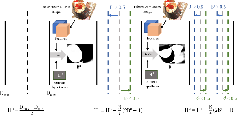
Figure 1: Visualization of IB-MVS depth inference algorithm for a single source image. The inverse depth range $[D_{\text{min}}$, $D_{\text{max}}]$ is explored iteratively by updating the inverse depth map hypothesis $H^{t}$ by means of the binary decision mask $B^{t}$ with $t=0,1,\ldots,T-1$.

3.3 Binary decision network

The decision network D-Net exhibits a U-Net [Ronneberger et al.(2015)Ronneberger, Fischer, and Brox]-like encoder-decoder structure and it is depicted in Figure 3. At the top level, the decoder is fed both with the feature maps $F_{r}$ and $F_{s}\in\mathbb{R}^{F\times M\times N}$, obtained by applying a Feature Pyramid Network [Gu et al.(2020)Gu, Fan, Zhu, Dai, Tan, and Tan] to the reference and source images $I_{r}$ and $I_{s}$, respectively, as well as with a depth map hypothesis $h\in\mathbb{R}^{M\times N}$. At each level of the encoder, deformable convolutions [Zhu et al.(2019)Zhu, Hu, Lin, and Dai] are used to convolve the source image feature maps along locations on the epipolar line determined by the depth hypothesis. Specifically, we deform a $k\times k$ kernel such that each of the $k^{2}$ sampling locations of the kernel correspond to locations on the epipolar line. We use kernel size $k=5$ and can thus center the deformed kernel on the epipolar line at the location predicted by the current depth hypothesis $h^{t}(i,j)$ and distribute the samples on either side spaced with a unit vector in pixel coordinates. The resulting sampled features from the source feature map are then concatenated with the reference feature map, as suggested in [Badki et al.(2020)Badki, Troccoli, Kim, Kautz, Sen, and Gallo]. This procedure is repeated at each resolution level, the resulting feature maps are further processed with standard convolutional layers and passed both to the next lower resolution level of the encoder and to the decoder, as depicted in Figure 3. At the decoder side, the feature maps are upsampled and further concatenated with the features from the encoder at the next higher resolution level. The output binary mask $B^{t}_{s}$ is generated using a sigmoid activation function. We include a detailed specification of the convolutional hyper-parameters in Section A of the supplementary material.

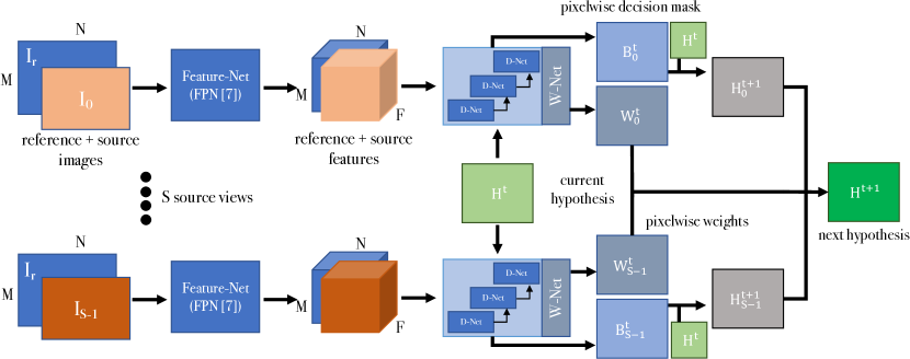
Figure 2: Architecture of the overall system. Deep features extracted from the reference and source images using a FPN architecture [Gu et al.(2020)Gu, Fan, Zhu, Dai, Tan, and Tan] are used as the input for three hierarchy levels of D-Nets, which predict the decision masks $B_{s}^{t}$. They are then used to compute the new inverse depth hypothesis $H_{s}^{t+1}$ for $s$. These are fused using weights $W_{s}^{t}$ estimated by W-Net and the fused result $H^{t+1}$ is the new inverse depth hypothesis for the next iteration.

In practice, in order to predict the binary decision mask $B_{s}^{t}$, we employ three D-Nets on full, half and quarter resolution inputs. In particular, as depicted in Figure 3, the output features from the previous scale D-Net are employed on the next scale. We observed that employing three resolution levels leads to higher quality binary decision masks. In fact, this choice increases the overall architecture receptive field and permits a coarse to fine refinement of the estimated masks, as each level employs the previous level output.

3.4 Fusion weights network

In the proposed architecture, each D-Net is followed by a W-Net, a network whose objective is to assign a confidence, in the form of a weight map, to the predicted binary decision mask. Figure 3 depicts W-Net in gray. Inspired by [Zhang et al.(2020)Zhang, Yao, Li, Luo, and Fang], W-Net operates on the pixelwise entropy of the predicted binary mask $E_{s}^{t}=-(B_{s}^{t}\log(B_{s}^{t})+(1-B_{s}^{t})\log(1-B_{s}^{t}))$. This design strategy, coupled with the choice to use the depth hypothesis to sample the source image, rather than as a network input, makes our overall algorithm scale independent. As suggested in [Zhang et al.(2020)Zhang, Yao, Li, Luo, and Fang], the final weight at the pixel $(i,j)$ is predicted as $W_{s}^{t}(i,j)=\exp(-w_{s}^{t}(i,j))$ where $w_{s}^{t}(i,j)$ is the network output. The pixelwise weights are used by our depth inference algorithm during the fusion stage in Eq. (3). The ideally predicted weights are small in those areas where the binary decision mask is not reliable, such as in occluded regions, and large otherwise, such that inverse depth hypotheses from different source images can complement each other. This approach mitigates the negative effect of potentially erroneous estimates $H_{s}^{t+1}$ from the source views, when fusing them into the new depth hypothesis $H^{t+1}$. This is crucial, as $H^{t+1}$ represents the starting point for the estimation of the next iteration binary decision masks.

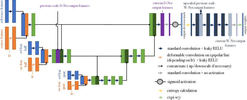
Figure 3: D-Net and W-Net architecture overview showing feature channel slices. The network uses standard 2D convolutions in combination with deformable 2D convolutions [Zhu et al.(2019)Zhu, Hu, Lin, and Dai] which utilize depth hypothesis $h^{t}$ to sample the epipolar line of the source image.

4 Experiments

In this section, firstly we describe the training procedure adopted for IB-MVS, then we compare it to state-of-the-art works on popular MVS benchmarks.

4.1 Network training

First, the multi-level D-Net is pre-trained on random uniform inverse depth map hypotheses with $H(i,j)=D_{\text{rand}}$ for every $(i,j)$ and $D_{\text{rand}}\in[D_{\text{min}},D_{\text{max}}]$, as proposed in [Badki et al.(2020)Badki, Troccoli, Kim, Kautz, Sen, and Gallo]. The ground truth binary decision mask $B_{\text{GT}}\in\mathbb{R}^{M\times N}$ for a given depth map hypothesis $h=1/H$ is computed from the ground truth depth map $d_{\text{GT}}$ using Equation (1). We employ a loss $L_{k}$ at each level $k=0,1,2$ of the multi-level D-Net, with $2$ being the full resolution. In particular, $L_{k}$ is defined as the average of the Binary Cross Entropy (BCE) at the valid pixels $(i,j)$:

$$L_{k}=\frac{1}{\overline{V}}\sum_{i,j}V(i,j)\>\text{BCE}(B(i,j),B_{\text{GT}}(i,j))\vspace{-5pt}$$ (4)

where $V=\sum_{i,j}V(i,j)$ with $V(i,j)$ equal to $1$ if the pixel has a valid ground truth depth, $0$ otherwise. The BCE loss in Eq. (4) is defined as follows:

$$\text{BCE}(b,b_{\text{GT}})=-(b_{\text{GT}}\log(b)+(1-b_{\text{GT}})\log(1-b)).$$ (5)

The overall loss is the weighted sum $L=\sum_{k=0}^{2}\lambda_{k}L_{k}$ with $\lambda_{0,1,2}=(0.25,0.5,1.0)$. After the pre-training, we train the multi-level D-Net using the depth inference algorithm described in Section 3.2 with $T=8$ iterations. However, we do not consider the fusion step at this stage and work with a single randomly selected source image over the $T$ iterations. The random selection of source images was shown to be beneficial by [Wang et al.(2021)Wang, Galliani, Vogel, Speciale, and Pollefeys]. We employ the previously introduced loss $L$ on each one of the binary decision masks $B_{s}^{t}$, with $t=0,1,...,T-1$, generated alongside the depth inference procedure. We refer to the loss at the iteration $t$ as $L^{t}$. At iteration $t$, the inverse depth hypothesis $H^{t}$ is used both by the multi-level D-Net to generate $B_{s}^{t}$ and in Eq. (1) to generate its ground truth. Now the loss $L^{t}$ can be computed and the next hypothesis $H^{t+1}$ generated. The procedure is iterated and the final loss is the sum over the $T$ losses $L^{t}$. We do not back-propagate across iterations. Finally, in the third training stage, we train W-Net jointly with D-Net. At this stage we fuse $B_{s}^{t}$ from $4$ randomly selected source images using the weights from W-Net with the same approach used to fuse the inverse hypotheses in Section 3.2 to generate $B^{t}$. We compute the loss $L^{t}$ of one iteration, where $t$ is randomly chosen in $\{0,\dots,T-1\}$, as the sum of losses on the $S$ individual $B_{s}^{t}$ and fused $B^{t}$. We implemented IB-MVS in PyTorch [Paszke et al.(2019)Paszke, Gross, Massa, Lerer, Bradbury, Chanan, Killeen, Lin, Gimelshein, Antiga, Desmaison, Kopf, Yang, DeVito, Raison, Tejani, Chilamkurthy, Steiner, Fang, Bai, and Chintala] and trained with batch size $1$ using ADAM [Kingma and Ba(2014)].

4.2 Evaluation metrics

In our evaluation, we present experimental results on three popular MVS benchmarks, namely DTU [Aanæs et al.(2016)Aanæs, Jensen, Vogiatzis, Tola, and Dahl], Tanks and Temples [Knapitsch et al.(2017)Knapitsch, Park, Zhou, and Koltun] and ETH3D high and low-res [Schöps et al.(2017)Schöps, Schönberger, Galliani, Sattler, Schindler, Pollefeys, and Geiger]. These benchmarks compare the reconstructed point cloud against a dense ground truth and extract completeness and accuracy metrics (recall and precision, respectively, for Tanks and Temples [Knapitsch et al.(2017)Knapitsch, Park, Zhou, and Koltun]). Completeness and accuracy are aggregated into a single metric: their average for DTU [Aanæs et al.(2016)Aanæs, Jensen, Vogiatzis, Tola, and Dahl] and harmonic mean, denoted F-score, for Tanks and Temples [Knapitsch et al.(2017)Knapitsch, Park, Zhou, and Koltun] and ETH3D [Schöps et al.(2017)Schöps, Schönberger, Galliani, Sattler, Schindler, Pollefeys, and Geiger]. For DTU [Aanæs et al.(2016)Aanæs, Jensen, Vogiatzis, Tola, and Dahl], accuracy and completeness are measured in mm, hence lower is better. For ETH3D [Schöps et al.(2017)Schöps, Schönberger, Galliani, Sattler, Schindler, Pollefeys, and Geiger] and Tanks and Temples [Knapitsch et al.(2017)Knapitsch, Park, Zhou, and Koltun], these metrics are percentages, hence higher is better.

4.3 Ablation study

We first investigate the influence of the iterations $T$ on the point cloud results for DTU [Aanæs et al.(2016)Aanæs, Jensen, Vogiatzis, Tola, and Dahl]. In Table 1, we show that increasing the number of iterations leads to improved results, which is coherent with our iterative depth refinement. The larger performance difference between $6-7$ iterations, compared to $7-8$ and $8-9$, is explained by the progressively shrinking step size of IB-MVS. Furthermore, we investigate the benefits of using our W-Net in the fusion step. In particular, we compare it to a naive strategy that simply averages the depth map hypotheses from the different source views. The results in Table 1 show that, for the same number of iterations $T=8$, W-Net leads to a better completeness and an overall better quality (avg. metric) than the naive fusion strategy, while exhibiting a competitive accuracy. The improved accuracy of the naive fusion strategy is obtained at the cost of worse completeness, as the absence of W-Net leads to more inconsistent estimates in occluded regions.

W-Net	T	avg.	acc.	cmp.	RT
✓	6	0.717	0.769	0.664	2.0s
✓	7	0.371	0.402	0.340	2.3s
✓	8	0.321	0.334	0.309	2.7s
-	8	0.342	0.326	0.359	2.3s
-	9	0.343	0.324	0.362	2.6s

Table 1: Ablation study on DTU test-set using accuracy, completeness and their average in mm (lower is better). We observe improvements with increasing iterations T. After T=8 the subdivision of the search space is sufficient, thus the result for T=9 is very close. Further, the inclusion of W-Net improves the results for the same number of iterations.

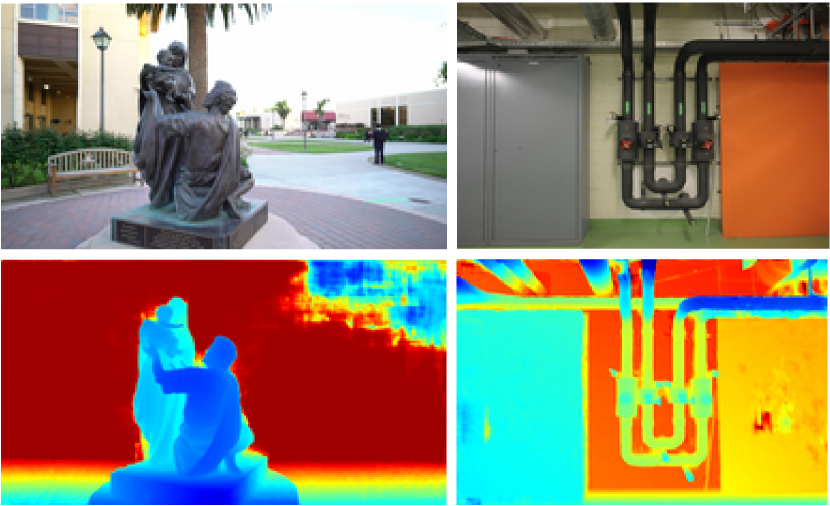
Figure 4: Qualitative depth map results from Tanks and Temples [Knapitsch et al.(2017)Knapitsch, Park, Zhou, and Koltun] and ETH3D [Schöps et al.(2017)Schöps, Schönberger, Galliani, Sattler, Schindler, Pollefeys, and Geiger].

4.4 Benchmark results

We use Tanks and Temples [Knapitsch et al.(2017)Knapitsch, Park, Zhou, and Koltun] and ETH3D [Schöps et al.(2017)Schöps, Schönberger, Galliani, Sattler, Schindler, Pollefeys, and Geiger] high and low-res in order to evaluate the generalization capabilities of IB-MVS, since we do not train on their respective training sets.

The feasible depth range $[d_{min},d_{max}]$ is inferred from the SfM model using the method in [Yao et al.(2018)Yao, Luo, Li, Fang, and Quan]. The computed depth maps are fused into a single point cloud with the proposed method of [Yao et al.(2018)Yao, Luo, Li, Fang, and Quan]; we denote its parameters representing the number of consistent views and the geometric re-projection error threshold as $S_{g}$ and $g$, respectively. We denote the used image resolution as $M\times N$, the runtime per image as $RT$ and the memory consumption as $MEM$. Finally, we recall that $S$ is number of used source views.

For the evaluation on the DTU benchmark, we train the network on DTU for ($8$, $12$, $2$) epochs and learning rates ($10^{-4}$, $10^{-4}$, $10^{-5}$) in the stages ($1$ $2$, $3$) described in Section 4.1, respectively. For the evaluations on Tanks and Temples and ETH3D, we train on DTU at stage $1$ and on Blended MVS [Yao et al.(2020)Yao, Luo, Li, Zhang, Ren, Zhou, Fang, and Quan] at stages $2$ and $3$, for ($8$, $21$, $4$) epochs using learning rates ($10^{-4}$, $10^{-4}$, $10^{-5}$). Every training on DTU employs the ground truth depth maps and train-test split of [Yao et al.(2018)Yao, Luo, Li, Fang, and Quan]. Finally, our method is run for $T=8$ iterations on DTU and for $T=9$ iterations on Tanks and Temples [Knapitsch et al.(2017)Knapitsch, Park, Zhou, and Koltun] and ETH3D [Schöps et al.(2017)Schöps, Schönberger, Galliani, Sattler, Schindler, Pollefeys, and Geiger]. All the experiments were performed using an Nvidia RTX 2080Ti graphics card.

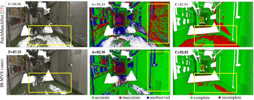
Figure 5: Point cloud comparison with PatchMatchNet [Wang et al.(2021)Wang, Galliani, Vogel, Speciale, and Pollefeys] on the ETH3D [Schöps et al.(2017)Schöps, Schönberger, Galliani, Sattler, Schindler, Pollefeys, and Geiger] high-res terrains dataset. We show the output point cloud, accuracy and completeness.

	low-res-test				low-res-train			high-res-test				high-res-train
publication	F	acc.	cmp.	RT	F	acc.	cmp.	F	acc.	cmp.	RT	F	acc.	cmp.
DeepC-MVS [Kuhn et al.(2020)Kuhn, Sormann, Rossi, Erdler, and Fraundorfer]	62.37	65.89	59.42	5746	61.99	65.98	59.27	87.08	89.15	85.52	3155	84.81	90.37	80.30
COLMAP [Schönberger et al.(2016)Schönberger, Zheng, Pollefeys, and Frahm]	52.32	61.51	45.89	3312	49.91	69.58	40.86	73.01	91.97	62.98	1658	67.66	91.85	55.13
ACMM [Xu and Tao(2019)]	55.01	52.37	58.27	1662	55.12	54.69	57.01	80.78	90.65	74.34	1165	78.86	90.67	70.42
PCF-MVS [Kuhn et al.(2019)Kuhn, Lin, and Erdler]	57.06	56.56	58.42	9289	57.32	57.03	58.17	80.38	82.15	79.29	2272	79.42	84.11	75.73
R-MVSNet [Yao et al.(2019)Yao, Luo, Li, Shen, Fang, and Quan]	36.87	37.45	37.16	2413	-	-	-	-	-	-	-	-	-	-
CasMVSNet [Gu et al.(2020)Gu, Fan, Zhu, Dai, Tan, and Tan]	44.49	55.44	38.80	-	49.00	62.06	41.86	-	-	-	-	-	-	-
MVSCRF [Xue et al.(2019)Xue, Chen, Wan, Huang, Yu, Li, and Bao]	28.32	34.84	24.97	-	-	-	-	-	-	-	-	-	-	-
P-MVSNet [Luo et al.(2019)Luo, Guan, Ju, Huang, and Luo]	44.46	54.95	38.28	627	-	-	-	-	-	-	-	-	-	-
BP-MVSNet [Sormann et al.(2020)Sormann, Knobelreiter, Kuhn, Rossi, Pock, and Fraundorfer]	43.22	32.65	64.34	-	50.87	49.12	55.29	-	-	-	-	-	-	-
Att-MVS [Luo et al.(2020)Luo, Guan, Ju, Wang, Chen, and Luo]	45.85	64.84	37.07	-	-	-	-	-	-	-	-	-	-	-
PVSNet [Xu and Tao(2020)]	45.78	38.39	57.76	2116	-	-	-	72.08	66.41	80.05	830	67.48	-	-
PMNet [Wang et al.(2021)Wang, Galliani, Vogel, Speciale, and Pollefeys]	-	-	-	-	-	-	-	73.12	69.71	77.46	493	64.21	64.81	65.43
IB-MVS (ours)	49.19	39.31	67.29	1487	55.84	61.06	52.66	75.85	71.64	82.18	616	71.21	75.21	69.02

Table 2: ETH3D [Schöps et al.(2017)Schöps, Schönberger, Galliani, Sattler, Schindler, Pollefeys, and Geiger] results: F-score, accuracy and completeness as percentage (2cm). Higher is better, overall best underlined, best among learning based in bold. For the test sets, we report the average per-scene runtime RT in seconds (for methods that provide this).

	DTU [Aanæs et al.(2016)Aanæs, Jensen, Vogiatzis, Tola, and Dahl]			Tanks and Temples [Knapitsch et al.(2017)Knapitsch, Park, Zhou, and Koltun]
	test			intermediate			advanced
publication	avg.	acc.	cmp.	F	preci.	reca.	F	preci.	reca.
DeepC-MVS [Kuhn et al.(2020)Kuhn, Sormann, Rossi, Erdler, and Fraundorfer]	-	-	-	59.79	59.11	61.21	34.54	40.68	31.30
ACMM [Xu and Tao(2019)]	-	-	-	57.27	49.19	70.85	34.02	35.63	34.90
COLMAP [Schönberger et al.(2016)Schönberger, Zheng, Pollefeys, and Frahm]	-	-	-	42.14	43.16	44.48	27.24	33.65	23.96
PCF-MVS [Kuhn et al.(2019)Kuhn, Lin, and Erdler]	-	-	-	55.88	49.82	65.68	35.69	37.52	35.36
R-MVSNet [Yao et al.(2019)Yao, Luo, Li, Shen, Fang, and Quan]	0.422	0.385	0.459	48.40	43.74	57.60	24.91	31.47	22.05
BP-MVSNet [Sormann et al.(2020)Sormann, Knobelreiter, Kuhn, Rossi, Pock, and Fraundorfer]	0.327	0.333	0.320	57.60	51.26	68.77	31.35	29.62	35.61
P-MVSNet [Luo et al.(2019)Luo, Guan, Ju, Huang, and Luo]	0.420	0.406	0.434	55.62	49.93	63.82	-	-	-
Att-MVS [Luo et al.(2020)Luo, Guan, Ju, Wang, Chen, and Luo]	0.356	0.383	0.329	60.05	61.89	58.93	31.93	40.58	27.26
CVP-MVSNet [Yang et al.(2020)Yang, Mao, Alvarez, and Liu]	0.351	0.296	0.406	54.03	51.41	60.19	-	-	-
CasMVSNet [Gu et al.(2020)Gu, Fan, Zhu, Dai, Tan, and Tan]	0.355	0.325	0.385	56.84	47.62	74.01	31.12	29.68	35.24
PatchMatchNet [Wang et al.(2021)Wang, Galliani, Vogel, Speciale, and Pollefeys]	0.352	0.427	0.277	53.15	43.64	69.37	32.31	27.27	41.66
UCS-Net [Cheng et al.(2020)Cheng, Xu, Zhu, Li, Li, Ramamoorthi, and Su]	0.344	0.338	0.349	54.83	46.66	70.34	-	-	-
LANet [Zhang et al.(2021)Zhang, Hu, Wang, Cao, and Zhang]	0.335	0.320	0.349	55.70	45.62	75.68	-	-	-
D2HC-RMVSNet [Yan et al.(2020)Yan, Wei, Yi, Ding, Zhang, Chen, Wang, and Tai]	0.386	0.395	0.378	59.20	49.88	74.08	-	-	-
VisMVSNet [Zhang et al.(2020)Zhang, Yao, Li, Luo, and Fang]	0.365	0.369	0.361	60.03	54.44	70.48	-	-	-
IB-MVS (ours)	0.321	0.334	0.309	56.02	47.71	72.64	31.96	27.85	41.48

Table 3: DTU [Aanæs et al.(2016)Aanæs, Jensen, Vogiatzis, Tola, and Dahl] results: accuracy, completeness and their average are in mm, lower is better. Tanks and Temples [Knapitsch et al.(2017)Knapitsch, Park, Zhou, and Koltun] results: precision, recall and F-score are percentages, higher is better. Overall best results are underlined, best among learning based methods are bold.

ETH3D benchmark [Schöps et al.(2017)Schöps, Schönberger, Galliani, Sattler, Schindler, Pollefeys, and Geiger]

This dataset is the most challenging one for learning-based MVS methods, especially the high-res subset. On the one hand, the high resolution of its images represents a memory bottleneck for learning-based cost-volume methods. On the other, it is characterized by images with wide baselines and with a significantly lower overlap than in Tanks and Temples [Knapitsch et al.(2017)Knapitsch, Park, Zhou, and Koltun] and DTU [Aanæs et al.(2016)Aanæs, Jensen, Vogiatzis, Tola, and Dahl], which can make matching without pixelwise source view selection difficult. For the high-res dataset we set $M\times N=1984\times 1312$, $S=4$, $S_{g}=1$, $g=1.0$ and obtain $RT=7.7s$, $MEM=7.9GB$. For the low-res dataset we set $M\times N=928\times 512$, $S=4$, $S_{g}=3$, $g=0.1$ and obtain $RT=1.5s$, $MEM=2.3GB$. We provide quantitative results for both the datasets in Table 2. Although this benchmark had been dominated by traditional methods such as ACMM [Xu and Tao(2019)] and DeepC-MVS [Kuhn et al.(2020)Kuhn, Sormann, Rossi, Erdler, and Fraundorfer] in the past, the recently published PatchMatchNet [Wang et al.(2021)Wang, Galliani, Vogel, Speciale, and Pollefeys] was able to achieve competitive results: IB-MVS outperforms [Wang et al.(2021)Wang, Galliani, Vogel, Speciale, and Pollefeys] on both the training and the test datasets. Learning-based approaches relying on cost-volumes are limited on this benchmark, however our iterative approach allows IB-MVS to infer accurate results, even on high resolution images. Further, since large viewpoint changes are present in this benchmark, the implemented fusion scheme allows IB-MVS to deal with occluded regions.

DTU benchmark [Aanæs et al.(2016)Aanæs, Jensen, Vogiatzis, Tola, and Dahl]

This dataset contains close-range images of various objects. For this dataset, we set $M\times N=1152\times 864$, $S=4$, $S_{g}=3$, $g=0.25$ and obtain $RT=2.7s$, $MEM=3.8GB$. In Table 3 we compare IB-MVS to the recent learning-based state-of-the-art methods. It can be observed that IB-MVS provides very competitive accuracy and completeness values: in particular it achieves a good trade-off between the two, which results in the best average score. Finally, we achieve a complete reconstruction, even with a strict filtering parameter $g$. This is due to IB-MVS ability to yield very precise results without the need to use large cost-volumes. This is especially important in the case of the DTU benchmark, where we target highly precise reconstructions of single objects.

Tanks and Temples benchmark [Knapitsch et al.(2017)Knapitsch, Park, Zhou, and Koltun]

The intermediate subset focuses on reconstructing small and large single objects, while the advanced subset consists of large scale indoor and outdoor scenes. In our experiments, we set $M\times N=1920\times 1056$, $S=4$, $S_{g}=4$, $g=0.5$ (interm.), $S_{g}=3$, $g=0.5$ (adv.) and obtain $RT=6s$, $MEM=6.4GB$. On the advanced subset, IB-MVS is competitive with other state-of-the-art learning-based methods such as CasMVSNet [Gu et al.(2020)Gu, Fan, Zhu, Dai, Tan, and Tan] and PatchMatchNet [Wang et al.(2021)Wang, Galliani, Vogel, Speciale, and Pollefeys], as shown in Table 3. Our iterative exploration of the hypothesis space, along with our pixelwise source view fusion, allows IB-MVS to achieve competitive results among learning based methods on the challenging advanced subset. A possible direction for improving the intermediate set results could be to employ a confidence measure for the final predicted depth map, to filter out inaccurate points ahead of the point cloud fusion, similarly to [Kuhn et al.(2020)Kuhn, Sormann, Rossi, Erdler, and Fraundorfer]. Another direction could consider the improvement of the core architecture, for instance, by incorporating a regularization stage. In particular, the binary decision mask prediction could be regularized by a differentiable CRF, such as [Sormann et al.(2020)Sormann, Knobelreiter, Kuhn, Rossi, Pock, and Fraundorfer].

Finally, we discuss IB-MVS runtime performance on ETH3D, measured as the per-scene runtime of the complete reconstruction, in seconds, including the point cloud fusion step. IB-MVS is faster than traditional methods on both ETH3D high-res and low-res, as shown in Table 2. It is noteworthy that the low-res scenes contain more images. While the learning-based method PM-Net [Wang et al.(2021)Wang, Galliani, Vogel, Speciale, and Pollefeys] yields a better runtime than IB-MVS, a direct comparison is difficult. In fact, the PatchMatch algorithm utilized within PM-Net [Wang et al.(2021)Wang, Galliani, Vogel, Speciale, and Pollefeys] operates at half-resolution and the full resolution is obtained via a subsequent up-sampling and refinement. Instead, IB-MVS operates at full resolution and does not perform an additional refinement. Furthermore, IB-MVS achieves a better F-score than PM-Net [Wang et al.(2021)Wang, Galliani, Vogel, Speciale, and Pollefeys] on ETH3D high-res. On low-res, IB-MVS offers a competitive runtime compared to learning-based methods. In terms of F-score, IB-MVS outperforms the fastest learning-based method P-MVSNet [Luo et al.(2019)Luo, Guan, Ju, Huang, and Luo], which does not participate on high-res.

5 Conclusion

We presented IB-MVS, a novel learning-based approach for MVS that explores the depth space iteratively in a binary decision fashion. IB-MVS couples the advantages of learning-based methods, such as learned input representations, with an efficient exploration strategy of the hypothesis space. In fact, IB-MVS can handle high resolution images, as it does not require a cost volume. In addition, IB-MVS benefits from a pixelwise source view fusion strategy. Extensive results show that IB-MVS achieves competitive results compared to state of the art methods on popular MVS benchmarks. Acknowledgement: This work has been supported by the FFG, Contract No. 881844: "Pro²Future".

Supplementary material

A Network architecture hyper-parameters

We provide the network hyper-parameters of D-Net and W-Net in Table 4 and Table 5, respectively. As specified in the main paper, we use three resolution levels $l=(0,1,2)$ at quarter, half and full resolution. For generating the image features $\text{Feat}_{r_{l}}$ and $\text{Feat}_{s_{l}}$, we utilize the FPN architecture of [Gu et al.(2020)Gu, Fan, Zhu, Dai, Tan, and Tan] and set the number of feature channels for each level $F_{l}=(32,16,8)$. Further, we replace the batch normalization [Ioffe and Szegedy(2015)] in the FPN [Gu et al.(2020)Gu, Fan, Zhu, Dai, Tan, and Tan] with instance normalization [Ulyanov et al.(2016)Ulyanov, Vedaldi, and Lempitsky]. We denote the entropy calculated from the output mask $B_{s_{l}}$ according to Section 3.4 of the main paper as $E_{s_{l}}$. In Tables 4 and 5, we denote 2D convolutions as 2D conv, deformable 2D convolutions [Zhu et al.(2019)Zhu, Hu, Lin, and Dai] as 2D def. conv and transposed 2D convolutions as 2D tran. conv. Further, we denote the leaky ReLU activation function as LReLU, the number of input and output channels with $\#C_{\text{in}}$ and $\#C_{\text{out}}$, the stride with str. and kernel size with $k$ (we add $\backslash b$ when no bias is used, the padding is set to $\frac{k-1}{2}$).

B Supplementary qualitative results

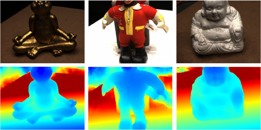
Figure 8: Qualitative depth map results for DTU [Aanæs et al.(2016)Aanæs, Jensen, Vogiatzis, Tola, and Dahl]. For each column, the reference image is at the top and the corresponding IB-MVS depth map at the bottom. Low to high depth values are color coded from blue to red.

In Figure 6, we provide qualitative point cloud results of our method IB-MVS for the DTU [Aanæs et al.(2016)Aanæs, Jensen, Vogiatzis, Tola, and Dahl], Tanks and Temples [Knapitsch et al.(2017)Knapitsch, Park, Zhou, and Koltun] and ETH3D [Schöps et al.(2017)Schöps, Schönberger, Galliani, Sattler, Schindler, Pollefeys, and Geiger] high and low-res datasets. Additionally, in Figure 8, we provide supplementary qualitative IB-MVS depth map results from the DTU [Aanæs et al.(2016)Aanæs, Jensen, Vogiatzis, Tola, and Dahl] dataset.

In order to provide further insights into IB-MVS, in Figure 7 we provide a visualization of its intermediate outputs at different iterations $t=0,1,4,8$. For each source image $I_{s}$, at iteration $t$ the hypothesis $h^{t}$ is used to compute the binary decision mask $B_{s}^{t}$ and the weight mask $W_{s}^{t}$ via D-Net and W-Net, respectively; this permits to compute the new reference depth map hypothesis $h_{s}^{t+1}$ using Eq. (2) of the main paper. The rows 2-5 of Figure 7 show $B_{s}^{t}$, $W_{s}^{t}$ and $h_{s}^{t+1}$ for the 4 source images and different values of $t$. The new reference image depth hypothesis $h_{s}^{t+1}$ are then fused into a single depth map $h^{t+1}$ using the weights $W_{s}^{t}$. The first row of Figure 7 shows the reference image along with $h^{t+1}$ for different values of $t$. We conclude by observing that, as desired, the weight masks in Figure 7 assign a low confidence to those areas of the reference image that are occluded in the source image, as these areas cannot be matched. This can be appreciated in the weight masks $W_{s}^{t}$ depicted in rows 2 and 3, where the area below the sofa and the left-most region (highlighted in yellow) of the reference image are dark because they are occluded in the respective source images.

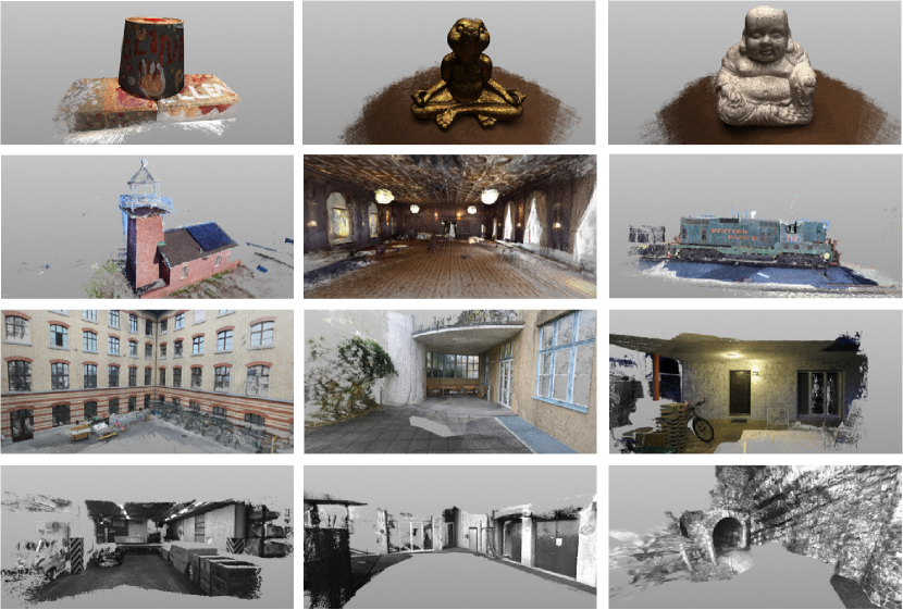
Figure 6: Qualitative point cloud results for DTU [Aanæs et al.(2016)Aanæs, Jensen, Vogiatzis, Tola, and Dahl] (first row), Tanks and Temples [Knapitsch et al.(2017)Knapitsch, Park, Zhou, and Koltun] (second row) and ETH3D [Schöps et al.(2017)Schöps, Schönberger, Galliani, Sattler, Schindler, Pollefeys, and Geiger] high and low-res (third and fourth row).

in name	out name	$\#C_{\text{in}}$	$\#C_{\text{out}}$	operation
$\text{Feat}_{r_{l}}$	Conv1	$F_{l}$	$F_{l}$	2D conv., k=3, str.=1, act.=LReLU
$\text{Feat}_{s_{l}}$	DConv1	$F_{l}$	$F_{l}$	2D def. conv., k=5, str.=1, act.=LReLU
Conv1 | DConv1	Conc1	$2F_{l}$	$2F_{l}$	concatenate along channel dim.
Conc1	Conv2	$2F_{l}$	$2F_{l}$	2D conv., k=3, str.=1, act.=LReLU
Conv2	Sc1	$2F_{l}$	$2F_{l}$	2D conv., k=3, str.=2, act.=LReLU
$\text{Feat}_{r_{l}}$	$\text{Feat}_{r_{l}}$ half	$F_{l}$	$F_{l}$	bilinear interp. downscale to half
$\text{Feat}_{s}{{}_{l}}$	$\text{Feat}_{s_{l}}$ half	$F_{l}$	$F_{l}$	bilinear interp. downscale to half
$\text{Feat}_{r_{l}}$ half	Conv3	$F_{l}$	$F_{l}$	2D conv., k=3, str.=1, act.=LReLU
$\text{Feat}_{s_{l}}$ half	DConv2	$F_{l}$	$F_{l}$	2D def. conv., k=5, str.=1, act.=LReLU
Conv3 | DConv2	Conc2	$2F_{l}$	$2F_{l}$	concatenate along channel dim.
Conc2	Conv4	$2F_{l}$	$2F_{l}$	2D conv., k=3, str.=1, act.=LReLU
Sc1 | Conv4	Conc3	$4F_{l}$	$4F_{l}$	for $l=0$ concatenate along channel dim.
Conc3	Conv5	$4F_{l}$	$4F_{l}$	for $l=0$ 2D conv., k=3, str.=1, act.=LReLU
$\text{Fo}_{l-1}$ | Sc1 | Conv4	Conc3	$4F_{l}+4F_{l-1}$	$4F_{l}+4F_{l-1}$	for $l>0$ concatenate along channel dim.
Conc3	ConvPr	$4F_{l}+4F_{l-1}$	$4F_{l}$	for $l>0$ 2D conv., k=3, str.=1, act.=LReLU
ConvPr	Conv5	$4F_{l}$	$4F_{l}$	for $l>0$ 2D conv., k=3, str.=1, act.=LReLU
Conv5	Sc2	$4F_{l}$	$4F_{l}$	2D conv., k=3, str.=2, act.=LReLU
$\text{Feat}_{r_{l}}$	$\text{Feat}_{r_{l}}$ quar.	$F_{l}$	$F_{l}$	bilinear interp. downscale to quarter
$\text{Feat}_{s}{{}_{l}}$	$\text{Feat}_{s_{l}}$ quar.	$F_{l}$	$F_{l}$	bilinear interp. downscale to quarter
$\text{Feat}_{r_{l}}$ quar.	Conv6	$F_{l}$	$F_{l}$	2D conv., k=3, str.=1, act.=LReLU
$\text{Feat}_{s_{l}}$ quar.	DConv3	$F_{l}$	$F_{l}$	2D def. conv., k=5, str.=1, act.=LReLU
Conv6 | DConv3	Conc4	$2F_{l}$	$2F_{l}$	concatenate along channel dim.
Conc4	Conv7	$2F_{l}$	$2F_{l}$	2D conv., k=3, str.=1, act.=LReLU
Sc2 | Conv7	Conc5	$6F_{l}$	$6F_{l}$	concatenate along channel dim.
Conc5	Conv8	$6F_{l}$	$6F_{l}$	2D conv., k=3, str.=1, act.=LReLU
Conv8	Conv9	$6F_{l}$	$6F_{l}$	2D conv., k=3, str.=1, act.=LReLU
Conv9	Conv10	$6F_{l}$	$6F_{l}$	2D conv., k=3, str.=1, act.=LReLU
Conv10	UConv1	$6F_{l}$	$6F_{l}$	2D tran. conv.,k=4$\backslash b$, str.=2, act.=LReLU
Conv5 | UConv1	Conc6	$10F_{l}$	$10F_{l}$	concatenate along channel dim.
Conc6	Conv11	$10F_{l}$	$4F_{l}$	2D conv., k=3, str.=1, act.=LReLU
Conv11	Conv12	$4F_{l}$	$4F_{l}$	2D conv., k=3, str.=1, act.=LReLU
Conv12	UConv2	$4F_{l}$	$4F_{l}$	2D tran. conv.,k=4$\backslash b$, str.=2, act.=LReLU
Conv2 | UConv2	Conc7	$6F_{l}$	$6F_{l}$	concatenate along channel dim.
Conc7	$\text{Fo}_{l}$	$6F_{l}$	$4F_{l}$	2D conv., k=3, str.=1, act.=LReLU
$\text{Fo}_{l}$	$B_{s_{l}}$	$4F_{l}$	$1$	2D conv., k=3$\backslash b$, str.=1, act.=sigmoid

Table 4: D-Net architecture hyper-parameters, specifying the convolution type, number of input and output channels, kernel size, stride and activation function.

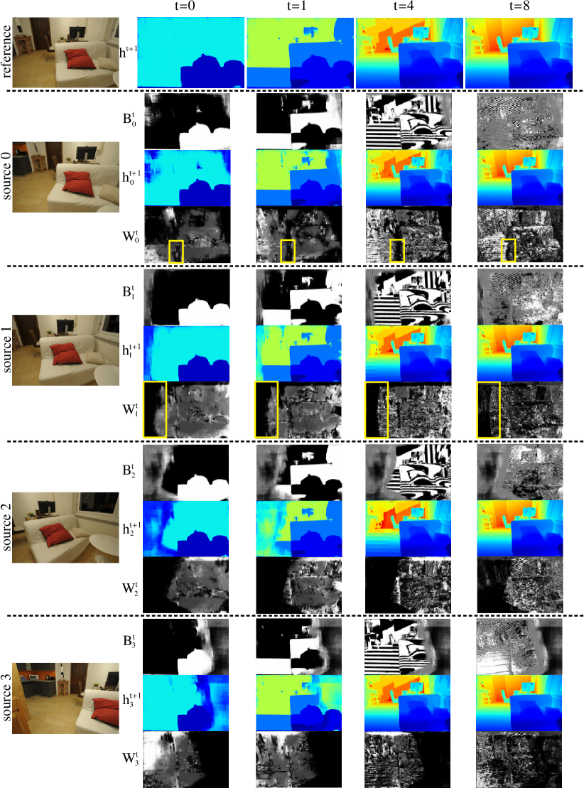
Figure 7: We visualize intermediate results of IB-MVS for a view of the ETH3D [Schöps et al.(2017)Schöps, Schönberger, Galliani, Sattler, Schindler, Pollefeys, and Geiger] high-res living room scene. The top row shows the depth hypothesis $h^{t+1}$ predicted at iteration $t$ by fusing the depth hypothesis $h_{s}^{t+1}$ from different source images according to $W_{s}^{t}$. We also show the binary decision masks $B_{s}^{t}$. We color code low to high depth values from blue to red. For $B_{s}^{t}$ and $W_{s}^{t}$ black represents the value $0$ and white represents the value $1$.

in name	out name	$\#C_{\text{in}}$	$\#C_{\text{out}}$	operation
$E_{s_{l}}$	Conv1	$1$	$2F_{l}$	for $l=0$ 2D conv., k=3, str.=1, act.=LReLU
$E_{s_{l}}$	Conv0	$1$	$F_{l}$	for $l>0$ 2D conv., k=3, str.=1, act.=LReLU
$\text{Fo}_{l-1}$	$\text{Fo}_{\text{Up}}$	$\frac{F_{l-1}}{2}$	$\frac{F_{l-1}}{2}$	for $l>0$ bilinear interp. upscale to double res.
$\text{Fo}_{\text{Up}}$	ConvPr	$\frac{F_{l-1}}{2}$	$F_{l}$	for $l>0$ 2D conv., k=3, str.=1, act.=LReLU
Conv0 | ConvPr	Conc1	$2F_{l}$	$2F_{l}$	for $l>0$ concatenate along channel dim.
Conc1	Conv1	$2F_{l}$	$2F_{l}$	for $l>0$ 2D conv., k=3, str.=1, act.=LReLU
Conv1	Conv2	$2F_{l}$	$2F_{l}$	2D conv., k=3, str.=1, act.=LReLU
Conv2	Conv3	$2F_{l}$	$F_{l}$	2D conv., k=3, str.=1, act.=LReLU
Conv3	$\text{Fo}_{l}$	$2F_{l}$	$\frac{F_{l}}{2}$	2D conv., k=3, str.=1, act.=LReLU
$\text{Fo}_{l}$	$w_{s_{l}}$	$\frac{F_{l}}{2}$	1	2D conv., k=3$\backslash b$, str.=1, act.=identity

Table 5: W-Net architecture hyper-parameters, specifying the convolution type, number of input and output channels, kernel size, stride and activation function.

References

- [Aanæs et al.(2016)Aanæs, Jensen, Vogiatzis, Tola, and Dahl] Henrik Aanæs, Rasmus Ramsbøl Jensen, George Vogiatzis, Engin Tola, and Anders Bjorholm Dahl. Large-scale data for multiple-view stereopsis. International Journal of Computer Vision, pages 1–16, 2016.
- [Badki et al.(2020)Badki, Troccoli, Kim, Kautz, Sen, and Gallo] Abhishek Badki, Alejandro Troccoli, Kihwan Kim, Jan Kautz, Pradeep Sen, and Orazio Gallo. Bi3d: Stereo depth estimation via binary classifications. In Proceedings of the IEEE Conference on Computer Vision and Pattern Recognition (CVPR), 2020.
- [Chen et al.(2019)Chen, Han, Xu, and Su] Rui Chen, Songfang Han, Jing Xu, and Hao Su. Point-based multi-view stereo network. In Proceedings of the IEEE International Conference on Computer Vision (ICCV), 2019.
- [Cheng et al.(2020)Cheng, Xu, Zhu, Li, Li, Ramamoorthi, and Su] Shuo Cheng, Zexiang Xu, Shilin Zhu, Zhuwen Li, Li Erran Li, Ravi Ramamoorthi, and Hao Su. Deep stereo using adaptive thin volume representation with uncertainty awareness. In Proceedings of the IEEE Conference on Computer Vision and Pattern Recognition (CVPR), 2020.
- [Galliani et al.(2015)Galliani, Lasinger, and Schindler] Silvano Galliani, Katrin Lasinger, and Konrad Schindler. Massively parallel multiview stereopsis by surface normal diffusion. In Proceedings of the IEEE International Conference on Computer Vision (ICCV), 2015.
- [Gallup et al.(2007)Gallup, Frahm, Mordohai, Yang, and Pollefeys] David Gallup, Jan-Michael Frahm, Philippos Mordohai, Qingxiong Yang, and Marc Pollefeys. Real-time plane-sweeping stereo with multiple sweeping directions. In Proceedings of the IEEE Conference on Computer Vision and Pattern Recognition (CVPR), 2007.
- [Gu et al.(2020)Gu, Fan, Zhu, Dai, Tan, and Tan] Xiaodong Gu, Zhiwen Fan, Siyu Zhu, Zuozhuo Dai, Feitong Tan, and Ping Tan. Cascade cost volume for high-resolution multi-view stereo and stereo matching. In Proceedings of the IEEE Conference on Computer Vision and Pattern Recognition (CVPR), 2020.
- [Huang et al.(2018)Huang, Matzen, Kopf, Ahuja, and Huang] Po-Han Huang, Kevin Matzen, Johannes Kopf, Narendra Ahuja, and Jia-Bin Huang. Deepmvs: Learning multi-view stereopsis. In Proceedings of the IEEE Conference on Computer Vision and Pattern Recognition (CVPR), 2018.
- [Ioffe and Szegedy(2015)] Sergey Ioffe and Christian Szegedy. Batch normalization: Accelerating deep network training by reducing internal covariate shift. In Proceedings of the 32nd International Conference on Machine Learning (ICML), 2015.
- [Ji et al.(2017)Ji, Gall, Zheng, Liu, and Fang] Mengqi Ji, Juergen Gall, Haitian Zheng, Yebin Liu, and Lu Fang. Surfacenet: An end-to-end 3d neural network for multiview stereopsis. In Proceedings of the IEEE Conference on Computer Vision and Pattern Recognition (CVPR), 2017.
- [Ji et al.(2020)Ji, Zhang, Dai, and Fang] Mengqi Ji, Jinzhi Zhang, Qionghai Dai, and Lu Fang. Surfacenet+: An end-to-end 3d neural network for very sparse multi-view stereopsis. In IEEE Transactions on Pattern Analysis and Machine Intelligence, 2020.
- [Kingma and Ba(2014)] Diederik P Kingma and Jimmy Ba. Adam: A method for stochastic optimization. arXiv:1412.6980 [cs.LG], 2014.
- [Knapitsch et al.(2017)Knapitsch, Park, Zhou, and Koltun] Arno Knapitsch, Jaesik Park, Qian-Yi Zhou, and Vladlen Koltun. Tanks and temples: Benchmarking large-scale scene reconstruction. ACM Transactions on Graphics, 36(4), 2017.
- [Kuhn et al.(2019)Kuhn, Lin, and Erdler] Andreas Kuhn, Shan Lin, and Oliver Erdler. Plane completion and filtering for multi-view stereo reconstruction. In Proceedings of the German Conference on Pattern Recognition (GCPR), 2019.
- [Kuhn et al.(2020)Kuhn, Sormann, Rossi, Erdler, and Fraundorfer] Andreas Kuhn, Christian Sormann, Mattia Rossi, Oliver Erdler, and Friedrich Fraundorfer. Deepc-mvs: Deep confidence prediction for multi-view stereo reconstruction. In Proceedings of the International Conference on 3D Vision (3DV), 2020.
- [Luo et al.(2019)Luo, Guan, Ju, Huang, and Luo] Keyang Luo, Tao Guan, Lili Ju, Haipeng Huang, and Yawei Luo. P-mvsnet: Learning patch-wise matching confidence aggregation for multi-view stereo. In Proceedings of the IEEE International Conference on Computer Vision (ICCV), 2019.
- [Luo et al.(2020)Luo, Guan, Ju, Wang, Chen, and Luo] Keyang Luo, Tao Guan, Lili Ju, Yuesong Wang, Zhuo Chen, and Yawei Luo. Attention-aware multi-view stereo. In Proceedings of the IEEE Conference on Computer Vision and Pattern Recognition (CVPR), 2020.
- [Paszke et al.(2019)Paszke, Gross, Massa, Lerer, Bradbury, Chanan, Killeen, Lin, Gimelshein, Antiga, Desmaison, Kopf, Yang, DeVito, Raison, Tejani, Chilamkurthy, Steiner, Fang, Bai, and Chintala] Adam Paszke, Sam Gross, Francisco Massa, Adam Lerer, James Bradbury, Gregory Chanan, Trevor Killeen, Zeming Lin, Natalia Gimelshein, Luca Antiga, Alban Desmaison, Andreas Kopf, Edward Yang, Zachary DeVito, Martin Raison, Alykhan Tejani, Sasank Chilamkurthy, Benoit Steiner, Lu Fang, Junjie Bai, and Soumith Chintala. Pytorch: An imperative style, high-performance deep learning library. Advances in Neural Information Processing Systems 32, 2019.
- [Ronneberger et al.(2015)Ronneberger, Fischer, and Brox] Olaf Ronneberger, Philipp Fischer, and Thomas Brox. U-net: Convolutional networks for biomedical image segmentation. In Proceedings of the International Conference on Medical Image Computing and Computer-Assisted Intervention (MICCAI), 2015.
- [Schönberger et al.(2016)Schönberger, Zheng, Pollefeys, and Frahm] Johannes Lutz Schönberger, Enliang Zheng, Marc Pollefeys, and Jan-Michael Frahm. Pixelwise view selection for unstructured multi-view stereo. In Proceedings of the European Conference on Computer Vision (ECCV), 2016.
- [Schöps et al.(2017)Schöps, Schönberger, Galliani, Sattler, Schindler, Pollefeys, and Geiger] Thomas Schöps, Johannes L. Schönberger, Silvano Galliani, Torsten Sattler, Konrad Schindler, Marc Pollefeys, and Andreas Geiger. A multi-view stereo benchmark with high-resolution images and multi-camera videos. In Proceedings of the IEEE Conference on Computer Vision and Pattern Recognition (CVPR), 2017.
- [Sormann et al.(2020)Sormann, Knobelreiter, Kuhn, Rossi, Pock, and Fraundorfer] Christian Sormann, Patrick Knobelreiter, Andreas Kuhn, Mattia Rossi, Thomas Pock, and Friedrich Fraundorfer. Bp-mvsnet: Belief-propagation-layers for multi-view-stereo. In Proceedings of the International Conference on 3D Vision (3DV), 2020.
- [Ulyanov et al.(2016)Ulyanov, Vedaldi, and Lempitsky] Dmitry Ulyanov, Andrea Vedaldi, and Victor S. Lempitsky. Instance normalization: The missing ingredient for fast stylization. arxiv:1607.08022 [cs.CV], 2016.
- [Vaswani et al.(2017)Vaswani, Shazeer, Parmar, Uszkoreit, Jones, Gomez, Kaiser, and Polosukhin] Ashish Vaswani, Noam Shazeer, Niki Parmar, Jakob Uszkoreit, Llion Jones, Aidan N Gomez, Łukasz Kaiser, and Illia Polosukhin. Attention is all you need. Advances in Neural Information Processing Systems 30, 2017.
- [Wang et al.(2021)Wang, Galliani, Vogel, Speciale, and Pollefeys] Fangjinhua Wang, Silvano Galliani, Christoph Vogel, Pablo Speciale, and Marc Pollefeys. Patchmatchnet: Learned multi-view patchmatch stereo. In Proceedings of the IEEE Conference on Computer Vision and Pattern Recognition (CVPR), 2021.
- [Xu and Tao(2019)] Qingshan Xu and Wenbing Tao. Multi-scale geometric consistency guided multi-view stereo. In Proceedings of the IEEE Conference on Computer Vision and Pattern Recognition (CVPR), 2019.
- [Xu and Tao(2020)] Qingshan Xu and Wenbing Tao. Pvsnet: Pixelwise visibility-aware multi-view stereo network. arXiv:2007.07714 [cs.CV], 2020.
- [Xue et al.(2019)Xue, Chen, Wan, Huang, Yu, Li, and Bao] Youze Xue, Jiansheng Chen, Weitao Wan, Yiqing Huang, Cheng Yu, Tianpeng Li, and Jiayu Bao. Mvscrf: Learning multi-view stereo with conditional random fields. In Proceedings of the IEEE International Conference on Computer Vision (ICCV), 2019.
- [Yan et al.(2020)Yan, Wei, Yi, Ding, Zhang, Chen, Wang, and Tai] Jianfeng Yan, Zizhuang Wei, Hongwei Yi, Mingyu Ding, Runze Zhang, Yisong Chen, Guoping Wang, and Yu-Wing Tai. Dense hybrid recurrent multi-view stereo net with dynamic consistency checking. In Proceedings of the European Conference on Computer Vision (ECCV), 2020.
- [Yang et al.(2020)Yang, Mao, Alvarez, and Liu] Jiayu Yang, Wei Mao, Jose M. Alvarez, and Miaomiao Liu. Cost volume pyramid based depth inference for multi-view stereo. In Proceedings of the IEEE Conference on Computer Vision and Pattern Recognition (CVPR), 2020.
- [Yao et al.(2018)Yao, Luo, Li, Fang, and Quan] Yao Yao, Zixin Luo, Shiwei Li, Tian Fang, and Long Quan. Mvsnet: Depth inference for unstructured multi-view stereo. In Proceedings of the European Conference on Computer Vision (ECCV), 2018.
- [Yao et al.(2019)Yao, Luo, Li, Shen, Fang, and Quan] Yao Yao, Zixin Luo, Shiwei Li, Tianwei Shen, Tian Fang, and Long Quan. Recurrent mvsnet for high-resolution multi-view stereo depth inference. In Proceedings of the IEEE Conference on Computer Vision and Pattern Recognition (CVPR), 2019.
- [Yao et al.(2020)Yao, Luo, Li, Zhang, Ren, Zhou, Fang, and Quan] Yao Yao, Zixin Luo, Shiwei Li, Jingyang Zhang, Yufan Ren, Lei Zhou, Tian Fang, and Long Quan. Blendedmvs: A large-scale dataset for generalized multi-view stereo networks. In Proceedings of the IEEE Conference on Computer Vision and Pattern Recognition (CVPR), 2020.
- [Zhang et al.(2020)Zhang, Yao, Li, Luo, and Fang] Jingyang Zhang, Yao Yao, Shiwei Li, Zixin Luo, and Tian Fang. Visibility-aware multi-view stereo network. In Proceedings of the British Machine Vision Conference (BMVC), 2020.
- [Zhang et al.(2021)Zhang, Hu, Wang, Cao, and Zhang] Xudong Zhang, Yutao Hu, Haochen Wang, Xianbin Cao, and Baochang Zhang. Long-range attention network for multi-view stereo. In Proceedings of the IEEE Winter Conference on Applications of Computer Vision (WACV), 2021.
- [Zhu et al.(2019)Zhu, Hu, Lin, and Dai] Xizhou Zhu, Han Hu, Stephen Lin, and Jifeng Dai. Deformable convnets v2: More deformable, better results. In Proceedings of the IEEE Conference on Computer Vision and Pattern Recognition (CVPR), 2019.