VPFNet: Improving 3D Object Detection with Virtual Point based LiDAR and Stereo Data Fusion

Abstract

It has been well recognized that fusing the complementary information from depth-aware LiDAR point clouds and semantic-rich stereo images would benefit 3D object detection. Nevertheless, it is not trivial to explore the inherently unnatural interaction between sparse 3D points and dense 2D pixels. To ease this difficulty, the recent proposals generally project the 3D points onto the 2D image plane to sample the image data and then aggregate the data at the points. However, this approach often suffers from the mismatch between the resolution of point clouds and RGB images, leading to sub-optimal performance. Specifically, taking the sparse points as the multi-modal data aggregation locations causes severe information loss for high-resolution images, which in turn undermines the effectiveness of multi-sensor fusion. In this paper, we present VPFNet—a new architecture that cleverly aligns and aggregates the point cloud and image data at the ‘virtual’ points. Particularly, with their density lying between that of the 3D points and 2D pixels, the virtual points can nicely bridge the resolution gap between the two sensors, and thus preserve more information for processing. Moreover, we also investigate the data augmentation techniques that can be applied to both point clouds and RGB images, as the data augmentation has made non-negligible contribution towards 3D object detectors to date. We have conducted extensive experiments on KITTI dataset, and have observed good performance compared to the state-of-the-art methods. Remarkably, our VPFNet achieves 83.21% moderate 3D AP and 91.86% moderate BEV AP on the KITTI test set, ranking the 1st since May 21th, 2021. The network design also takes computation efficiency into consideration – we can achieve a FPS of 15 on a single NVIDIA RTX 2080Ti GPU. The code will be made available for reproduction and further investigation.

I Introduction

Accurate and timely 3D object detection is an important yet challenging problem in many real-world 3D vision applications, including autonomous vehicles, domestic robots, virtual reality, etc. As explored in the literature, 3D object detectors can be developed combining data from different sensors, such as monocular images [1], stereo images [2, 3] and LiDAR point clouds [4, 5]. Although significant progress have been witnessed, the detection accuracy achieved by individually processing data of a single sensor is far from sufficient, due to the limitation of each sensor. For example, the RGB images are rich in semantic attributes, but lack depth information; the point clouds offer precise distance measurements, but cannot provide semantic information like colors, textures, and fine-grained shapes.

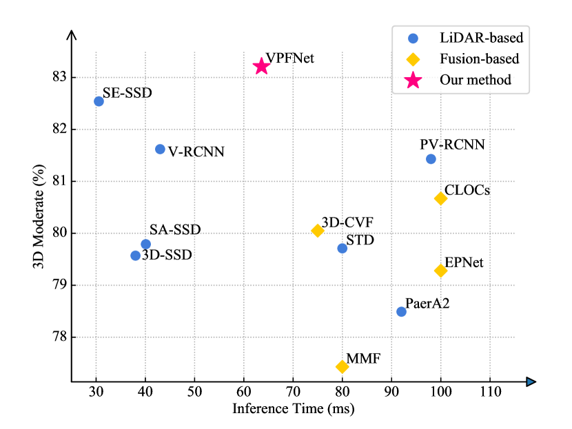
Figure 1: Our proposed VPFNet achieves the highest accuracy in 3D object detection for the moderate of car category on the KITTI [6] benchmark. Compared with the other multi-modal 3D object detection methods (marked in yellow), VPFNet achieves a competitive inference time of 63.6ms. Please refer to Table II for a more comprehensive performance comparison.

In light of the properties of RGB images and LiDAR point clouds, several innovations have been made to leverage their complementary information These multi-modal approaches can generally be categorized into two groups: object-level fusion [7, 8, 9, 10, 11, 12, 13] and point/voxel-level fusion  [14, 15, 16, 17, 18, 19, 20] according to the fusion granularity.

The first group of schemes combines the features at the object or region of interest (RoI) level. For example, AVOD [7] combines each object’s intermediate RoI features including image features and point cloud bird’s eye view (BEV) features via simple feature concatenation. SIFRNet [13] utilizes image features and frustum point clouds to generate 3D detection results following [10]. These schemes combine high-level, coarse-grained features, implicitly encoding the geometry information into the RoI context.

The second group of schemes conducts point/voxel level fusion, exploiting information fusion at a much finer granularity. For example, PointPainting [17] projects LiDAR points to the image plane, and retrieves the classification information from image semantic segmentation. EPNet [15] also projects points to the image plane, retrieving image features instead of semantic masks. 3D-CVF [14] constructs a 3D volume, and maps image features to the BEV plane. Multi-Task Multi-Sensor Fusion (MMF) [16] projects the 2D depth maps to the 3D space and forms pseudo LiDAR point clouds, then performs continuous fusion [18] at multiple granularities.

In this work, we take the point/voxel-level fusion approach in favor of its fine fusion granularity. These schemes usually involve combining low-level multi-modal features at 3D points or 2D pixels. However, as pointed out in [21], these schemes usually face a problem referred to as “resolution mismatch”. That is, the mismatch between dense image pixels and sparse LiDAR points renders that only a small portion of pixels have matching points.

We further illustrate the problem in Figure 2. It shows a black car that is more likely to absorb the laser energy, causing resolution mismatch. In fact, on the KITTI dataset, a Velodyne-64 LiDAR point cloud has only 20,000 points on the camera view while an image has more than 300,000 pixels. If we directly project 3D point clouds to the 2D plane and sample the features at matching image pixels [17], we will have a rather low sampling rate for image data, roughly 6.7%. Such a low sampling rate leads to serious information loss in the image plane.

Here, as an alternative approach, we could try to lift 2D image features to the 3D space as in [14]. However, naively associating the 2D pixels with the entire 3D space, this approach will significantly increase the processing demand. In consideration of computation efficiency, these schemes usually need to down-sample the aggregated features, e.g., further projecting these features to the BEV plane for subsequent processing. In this case, we may lose valuable 3D information.

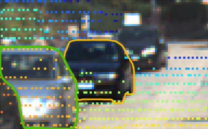
Figure 2: Illustration of resolution mismatch on the KITTI dataset. The car marked in orange contains 23 LiDAR points and more than 900 pixels. With the current sensor technology, pixel density is usually much higher than the point density.

To address this dilemma, we cleverly employ a set of “virtual” points in the 3D space that act as the multi-modal data aggregation points, whose density is in between pixel density and point density, $D_{point}<D_{virtual}<D_{pixel}$. For example, in our implementation, the density of virtual aggregation points is roughly $20$ times the density of actual LiDAR points in foreground areas. In this way, we can effectively bridge the resolution gap between the two sensors. When we project virtual points to the image plane, the resulting image data sampling rate will be higher.

However, when we try to use virtual points to aggregate corresponding LiDAR point data, a new challenge arises – virtual points are not directly associated with any point cloud features. To solve this challenge, we leverage the voxel-RoI pooling operation discussed in [22] that can locate the $K$ nearest point neighbors in the 3D space for a given location. By aggregating $K$ nearby point features to the virtual point, we also effectively replicate the sparse point cloud features, essentially leading to a much denser point cloud features.

Using virtual points to aggregate multi-modal data for the first time, we refer to our method as virtual-point fusion, VPFNet in short. In addition to the novel virtual-point aggregation, we also explore several multi-modal data augmentation techniques. Multi-modal detectors often face the difficulty of applying data augmentation to both types of sensor data, such as global rotation augmentation and ground truth boxes sampling augmentation. We carefully extend these techniques to multi-modal cases. Our evaluation results on KITTI show that VPFNet is ranked the highest for the following three test scenarios: $AP_{3D}$ moderate (83.21%), $AP_{BEV}$ moderate (91.86%), and $AP_{BEV}$ hard (86.94%). Our test performance on $AP_{3D}$ hard (78.20%) is ranked the highest among all the published results. Further, compared with our point cloud only network Voxel-RCNN [22], VPFNet can improve the $AP_{3D}$ value by $0.12\%$, $1.59\%$, and $1.14\%$ for easy, moderate, and hard on the car category, respectively. In Figure 1, we show the performance (both $AP_{3}D$ moderate accuracy and inference time) of VPFNet and several recent 3D detection networks (including both fusion-based networks and LiDAR-based networks) – VPFNet has the most accurate detection among them all, and its inference latency is the lowest among all the fusion-based detectors.

To summarize, this paper has the following contributions:

• We devise an accurate two-stage voxel-level stereo-LiDAR fusion framework, VPFNet, to effectively alleviate the resolution mismatch problem in fusing LiDAR and camera data. Easing this problem can nicely balance high sensor data sampling rate and high computation efficiency.

• We explore several techniques to optimize our VPFNet network, including random 3D proposal resizing to prevent over-fitting, weighted multi-branch combination to prevent single-modality dominance, and cut-n-paste based data augmentation.

• Over the popular KITTI dataset, we have carefully evaluated our 3D detection network. The results show that VPFNet delivers the best performance in several test scenarios. Moreover, with our light-weight design, the above accuracy can be achieved at a processing rate of 15 FPS.

II Related Work

In this section, we present the background and related work for the following related topics: (1) LiDAR-only 3D object detection, (2) Stereo-only 3D object detection, (3) LiDAR and camera fusion based 3D object detection (4) Augmentation for 3D Object detection

3D Object Detection Using LiDAR Only: As far as LiDAR-based 3D object detection is concerned, there are two mainstream models: point-based models and voxel-based models. Point-based methods [23, 24, 25] use point set abstraction to sample a fixed number of points as keypoints, and aggregate point features around keypoints with ball query. The keypoints preserve the original location information. However, since the point clouds are in-ordered, the complexity of point query is O(N), where N denotes the number of point clouds.

Voxel-based models [26, 27, 28] transfer raw-points to voxels. Voxel representation keeps the memory locality [29], while loses the original location information. SECOND [27] introduces a novel sparse convolution layer targeted at LiDAR point clouds. Voxel-RCNN  [22] devises voxel query to take the place of ball query, and achieves the state-of-the-art accuracy and high efficiency on the KITTI benchmark.

The above studies consider how to effectively perform 3D object detection usinwg LiDAR point clouds. Our work shows that by considering both RGB images as well as point clouds, we can achieve better 3D detection performance.

3D Object Detection Using Stereo Only: There are several works that lift stereo images to the 3D space. They can be divided into two groups. One is point based methods [30, 31, 32]. These methods generate intermediate 3D structure of pseudo LiDAR point clouds by depth estimation, and feed the points into LiDAR-only 3D detectors. These methods generate huge amount of pseudo points and is time-consuming.

Another group constructs cost volume in 3D space. For example, PLUME [3] constructs feature volume in 3D space and compresses it to BEV, then applies 2D convolution network to generate final results. The recently proposed two-stage method RTS3D [2] constructs instance level volumes using proposals, and uses an attention module and MLPs to get the final results.

The above studies consider how to effectively perform 3D object detection using stereo images in 3D space. Our work shows that by considering both RGB images as well as point clouds, we can achieve better 3D detection performance.

3D Object Detection Using Both LiDAR and Cameras: Several multi-modal 3D object detection networks have been proposed [33]. There are two levels of fusion: object level fusion [7, 8, 9, 10, 11, 12, 13] and point/voxel level fusion [14, 15, 16, 17, 18, 19, 20]. Object level fusion methods fuse in a coarse granularity. For example, AVOD [7] fuses features extracted from LiDAR BEV point clouds and camera front-view image and feed the features into fused RPNs for object detection; SIFRNet [13], F-ConvNet [9] utilize front view images and frustum point clouds to generate 3D detection results following [10]; CLOCs [11] encodes an object’s 2D and 3D detection results into a sparse tensor, and uses a 2D convolution network to refine the result.

The second group of schemes conduct point/voxel level fusion methods, they explicitly project the data between the 2D and 3D space, and fuse in a much finer granularity. For example, PointPainting [17] and EPNet [15] project LiDAR points to the image plane, and retrieve segmentation masks or image features. The point clouds are decorated with the retrieved features/masks. continuous-fusion [18] associates image features and point cloud features by adopting KNN search, and uses the non-empty neighbour features to be the empty voxel feature. These methods exploit only the sparse information contained in a dense image, and suffer from information loss. The problem is referred to as resolution mismatch [21].

3D-CVF [14] constructs a high resolution 3D voxel space and lifts image features to the dense 3D voxel space via camera matrix. To avoid expensive 3D convolution, it compresses the height channel and converts 3D voxels to BEV feature map, and loses the 3D information. To explore fusion in the second stage, 3D-CVF divides the proposal into grid points and projects them to the image plane and retrieves 2D image features. However, the extracted 2D image features are directly aggregated by PointNet [34] without any interaction with the 3D space.

MMF [16] aims at multiple relevant tasks learning. It exploits depth estimation and converts depth maps into pseudo-LiDAR points. The computation overhead is heavy if pseudo-LiDAR points are generated at pixel-level.

Building upon the success of the above pixel-level fusion schemes, we further consider how to bridge the resolution mismatch of these two modalities by employing “virtual” points in the 3D space. Our work shows that this step can lead to improved detection performance.

Augmentation for 3D Object Detection: As proposed in [35], popular point cloud augmentations include global rotation, global flipping, global scaling, and GT-sampling. These augmentations can accelerate convergence and boost the detection performance [27]. For global augmentations, they are reversible, and can be easily applied to fusion. However GT-sampling is not designed for multi-modal fusion. Some existing works try to avoid multi-modal GT-sampling by training with only global augmentation [15], or using GT-sampling only when the LiDAR backbone network was pretrained [14]. Recently, a new cut-n-paste based scheme was proposed in [36]. Inspired by [37], it cuts point cloud and image patches of ground-truth objects and pastes them into different scenes during training.

In addition to the above augmentations, we further employ a cut-n-paste based object sampling scheme that leverages the masks from prediction. Our work shows that this augmentation technique can effectively improve the performance.

III Preliminaries on Point/Voxel-Level LiDAR-Camera Fusion

Since VPFNet performs sensor fusion at the point/voxel level, we now provide a background overview on the architecture of this approach. A typical point/voxel level fusion scheme [17, 15, 18] consists of four steps: (1) 3D to 2D projection, (2) 2D feature sampling, (3) multi-modal data aggregation, and (4) 3D object detection.

Existing schemes often directly use LiDAR points as multi-modal data aggregation points [17, 15, 20]. They project the LiDAR point $P$ to the image plane as follows:

$$z_{c}\left[\begin{matrix}u\\ v\\ 1\end{matrix}\right]=hK\left[\begin{matrix}R&T\end{matrix}\right]\left[\begin{matrix}P_{x}\\ P_{y}\\ P_{z}\\ 1\end{matrix}\right],$$

where $P_{x},P_{y},P_{z}$ denote $P$’s 3D location, $u,v,z_{c}$ denote the 2D location and the depth of its projection on the image plane, $K$ denotes the camera intrinsic parameter, $R$ and $T$ denote the rotation and the translation of the lidar with respect to the stereo camera reference system. and $h$ denotes the scale factor due to down-sampling.

Then the corresponding image features at location $(u,v)$, $F_{u,v}$, can be sampled with bilinear interpolation. The sampled feature is then concatenated with point $P$’s own location and feature to form an aggregated feature vector. Figure 3 illustrates this process.

For example, in PointPainting [17], it aggregates the feature vector with a simple concatenation operation as follows:

$$\bm{\phi}_{P}=\text{concat}\{P_{x};P_{y};P_{z};P_{i};mask_{(u,v)}\},$$

where $\bm{\phi}_{P}$ is the aggregated feature vector at LiDAR point $P$, $P_{x}$, $P_{y}$, $P_{z}$, $P_{i}$ are the 3D coordinates, and intensity of point $P$, $mask_{(u,v)}$ is the sampled image segmentation mask. As another example, EPNet [15] utilizes a L1-fusion block to aggregate the multi-modal data in a feature vector.

Finally, the aggregated feature vectors are fed to the detection head. The final box classification and regression results are generated accordingly.

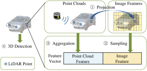
Figure 3: In a point/voxel level fusion scheme, the original or downsampled LiDAR points are projected to the 2D plane, to retrieve the corresponding 2D image features. The multi-modal features are then aggregated by concatenation for subsequent 3D object detection.

IV Virtual-Point Fusion ( VPFNet)

In this section we present the design of VPFNet. We first give the design overview, and then describe the important components one by one.

IV-A Design Overview

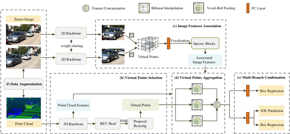
Figure 4: The architecture of the proposed VPFNet. Each dashed line box is associated with a subsection in Sec IV. Given a stereo and LiDAR point cloud pair, we first use (f) multi-modal data augmentation techniques to obtain an augmented scene in the training stage. Then in (b) virtual point selection, we feed the data into the 2D and 3D backbones separately. The 2D backbone is used only for feature extraction, and the 3D backbone is for generating the 3D proposals. The 3D proposals are randomly resized and divided into fixed-sized grid blocks, and the resulting vertices of each grid block/cell are virtual points. Then in (c) image feature association, the virtual points are projected to the image plane to sample the 2D image features. The sampled image features are thus associated with the virtual point. These features are voxelized and processed by stacked sparse convolution layers. Next, in (d) virtual points aggregation,we sample the virtual points as query points, and locate the $K$ nearest LiDAR point neighbors in the 3D space, and aggregates their features with the associated images, resulting in an aggregated feature vector. Finally In (e) multi-branch combination, these feature vectors are fed into the detection head to predict the final results. We also involve an auxiliary branch that only processes the aggregated image features to prevent single-modality dominance. Please note that the augmentation step and the proposal resizing step are only needed in the training stage.

We illustrate our multi-modal 3D detection network in Figure 4. The primary principle in designing VPFNet is to (1) carefully bridge the resolution gap between LiDAR point clouds and camera images, and (2) balance the sampling rate needed for detection accuracy and computation efficiency.

The first design choice is to determine whether we project 3D data to 2D to perform fusion, or vice versa. Considering the properties of images and point clouds (summarized in Table I), we choose to aggregate the sensor data in the 3D space. In this way, we can involve most of the point cloud information in the processing and avoid scale effect. Scale effect means an object’s 2D area size is related with both its actual sizes and depth. In general, LiDAR points are much more sparse than image pixels and contain less redundancy. They also give more accurate 3D detection results than images. As such, we argue that a fusion network needs to keep as much point cloud information as possible.

The second design choice is to determine at what locations in the 3D space to aggregate the data from both sensors. In order to bridge the resolution gap between the two, we choose to do so at virtual points that are sparser than image pixels but denser than LiDAR points. Given a virtual point, we need to find the corresponding image features and point cloud features, and suitably aggregate them. For image features association, we project the virtual point’s location to the 2D image plane, and retrieve the left/right image features accordingly. For point cloud features association, we perform a voxel-RoI pooling operation [22] to locate neighbors and aggregate their features. In this way, we sample the dense image features while aggregating/replicating the sparse point cloud features, nicely balancing the disparity in their resolutions.

	Point Cloud	Image
Feature Aggregation	3D neighbours	2D neighbours
Permutation	invariant [34]	variant
Scale Effect	no	yes
Memory Access	unordered [29]	ordered
Resolution	sparse	dense

TABLE I: Comparison of point clouds and images

Specifically, as shown in Figure 4, our network has the following main components:

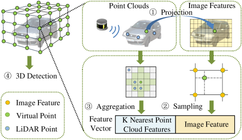
Figure 5: In VPFNet, we use virtual points (marked in green) to aggregate the multi-modal data. Virtual points are projected to the image plane to sample image features. As far as LiDAR point cloud features, we perform a voxel-RoI pooling operation (marked by the $5\times 5$ square) to aggregate point cloud features from $K$ nearest neighbors. The feature vector at each virtual point thus consists of the sampled image feature and aggregated $K$ point cloud features.

1. Virtual Points Selection. This step selects the virtual points from 3D proposals. Specifically, we feed point clouds into 3D backbone networks and generate 3D proposals, randomly resize the 3D proposals for better robustness, and divide them into discrete grid blocks. We then use the resulting grid points as virtual points (see Figure 5).

2. Associating Image Features to Virtual Points. This step samples the image features and associates the sampled image features to virtual points. Firstly we generate 2D image features with a light-weight 2D backbone. Then we sample the image features through virtual point projection. We voxelize and convolve the sampled image feature vectors through stacked sparse convolution layers to extract more compact features.

3. Aggregating LiDAR Point Features at Virtual Points. This step aggregates suitable LiDAR features to each virtual point. We first use a modified voxel-RoI pooling layer to query and aggregate the sparse LiDAR point cloud features. Both LiDAR point cloud features and image features are aggregated in a multi-scale manner.

4. Weighted Multi-Branch Combination. This step predicts the final results. Here we consider the main branch as well as an auxiliary branch to avoid single-modality dominance and alleviate over-fitting. Both branches predict the final results, while supervised with different weights.

5. Data Augmentation. This step performs suitable multi-modal data augmentation.

IV-B Virtual Points Selection

The sample density of LiDAR point clouds is much lower than that of camera images, especially for faraway objects and black objects (see Figure 2). Due to the severe resolution imbalance, traditional fusion schemes often lead to low sampling rate for image features, which likely hurts the overall detection performance.

To alleviate this problem, we do not use actual LiDAR points as multi-modal feature aggregation points, but propose to leverage virtual points (we sometimes refer to them as virtual points). The density of such virtual points is in between that of actual LiDAR points and image pixels. By attaching the suitable image features and point features to these virtual points, we can effectively increase the image feature sampling rate, better match the two types of data, and utilize more multi-modal features in the 3D detection.

Next, we explain how we select virtual points in the 3D space. Firstly, we feed LiDAR point clouds into the 3D backbone network to generate 3D proposals and 3D feature maps. Backbone refers to the network which takes the raw data as input and extracts the feature map upon which the rest of the network is based. 3D proposals refer to 3D candidate bounding boxes of the final detection that need to be verified in the refinement stage. The 3D backbone network we use has the same structure as Voxel-RCNN in [22]. The 3D proposals go through a non-maximum suppression (NMS) stage, while being ranked according to their intersection over union (IoU) with the ground truth. Only those proposals that have an IoU larger than a preset threshold will be selected. The proposals are further expanded by 0.8m in all dimensions to cover more contextual information.

The virtual points are selected from within these proposals. Since the proposals from point clouds are usually rather accurate, directly using them could potentially lead to over-fitting. Therefore, we randomly resize the 3D proposals to boost the overall robustness of the model.

Specifically, for each dimension of a 3D proposal, VPFNet randomly picks a noise value from a uniform distribution and adds that noise value to the original coordinate following the formulation below:

$$\Delta k=\phi\{u_{k}\},k\in\{x,y,z,w,h,l,\theta\},$$

where $\Delta k$ denotes the noise value in each dimension, and $\phi$ is a uniform distribution from $-u_{k}$ to $u_{k}$ ($u_{k}$ is varied according to different $k$), and $k$ denotes the seven dimensions of a box, including its box center location x, y, z, box dimensions width, length, height, and $\theta$. $\theta$ denotes the orientation angle of each box from the bird’s eye view. For each dimension $u_{k}$ is different. In Section V we show that this proposal box resizing augmentation is rather effective.

After random resizing, the proposals are divided to $N_{x}\times N_{y}\times N_{z}$ 3D grids along the length, width and height dimensions similar to [22]. We then use these grid points as the virtual points. Here, example $N_{x}$, $N_{y}$, and $N_{z}$ values are 12, 8, and 22, resulting in more than 2K samples in a foreground area. Such a sample density is much higher than that of the original LiDAR point clouds (typically hundreds of samples).

IV-C Associating Image Features to Virtual Points

Given a virtual point, we first locate the corresponding image features and associate them to the virtual point.

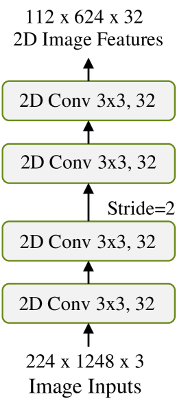
(a) 2D backbone

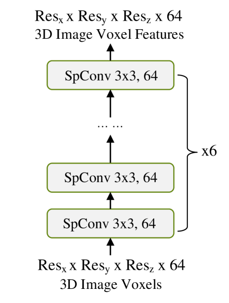
(b) 3D spconv block

Figure 6: The architecture of our 2D backbone (a) and 3D sparse convolution block (b). The output of the 2D backbone is down-sampled by two times compared with its input.

For 2D image feature extraction, we use two light-weight 2D convolution backbone networks. Following [2, 38], our 2D backbones are weight sharing. Figure 6(a) illustrates our 2D backbone structure. Our 2D backbone consists of four convolution layers, with all the convolution layers having a kernel size of 3$\times$3, and the second layer having a stride of 2. The generated feature maps are thus 2$\times$ down-sampled compared to the original resolution.

We then attach the sampled left and right image features to the virtual point $V$:

$$\bm{\phi_{V}}=\text{concat}\{I_{l};I_{r};V_{x};V_{y};V_{z}\},$$

where $\bm{\phi}_{V}$ is the resulting feature vector after aggregating the image features associated with $V$ located at $(V_{x},V_{y},V_{z})$, $I_{l}$ is the left image feature, $I_{r}$ is the right image feature.

After aggregating the image features to the feature vector $\bm{\phi_{V}}$ at the virtual point, VPFNet next voxelizes the feature vectors at all virtual points and performs feature extraction. In consideration of both information loss and computation efficiency, we choose to employ a light weight module that consists of six sparse convolution blocks [27] for feature extraction. Figure 6(b) illustrates our sparse convolution structure. All six spconv layers are standard 3$\times$3 convolution layers. We obtain the following image feature map $D_{0}$:

$$D_{0}=SPCONV(\Phi),$$

where $\Phi$ is the universe set of all aggregated feature vectors, $SPCONV$ is the employed sparse convolution operation.

IV-D Aggregating LiDAR Point Features to Virtual Points

Now we aggregate corresponding LiDAR point features to the virtual point. To compensate for the low sample density of LiDAR points, we locate multiple nearby LiDAR points and aggregate their features at a virtual point. In this way, the LiDAR points’ features are suitably replicated, effectively boosting the point cloud feature density. In order to find the nearby $k$ LiDAR points, we adopt the voxel-RoI pooling operation proposed in [22]. To reduce the complexity, the query points here has a resolution of $G_{x}\times G_{y}\times G_{z}$, where $G_{x}\times G_{y}\times G_{z}$ is the number of grid points within a 3D proposal. It is smaller than the resolution in last subsection.

We next explain how we modify voxel-RoI pooling to fit our problem. Given a virtual point, we query and aggregate its feature neighbours on the feature map. Considering that the feature maps in VPFNet are multi-modal and multi-scale, we execute queries on each feature map separately to pool the neighbouring features. The feature maps we use here in VPFNet include the image feature map $D_{0}$, and LiDAR point cloud feature maps $D_{1}$ and $D_{2}$, with $D_{1}$ being the 4x down-sampled feature map from our 3D backbone and $D_{2}$ the 8x down-sampled feature map. The queried neighbours are then aggregated by accelerated PointNet [22]. The aggregated features are of the same shape, and can be easily concatenated. Accordingly, we update the aggregated feature vector as:

$$\bm{\phi_{V}}=\text{concat}\{Q^{k}(D_{i})\},$$

where $D_{i}$ denotes the feature maps (3 feature maps in total as explained above), $Q^{k}$ denotes the query operated on different down-sampling scales (2 scales in total, detailed in Section V). $\text{concat}{\cdot}$ denotes feature concatenation. For a voxel query $Q$, given a virtual point $v$, and a voxel feature map $\bm{D}$, it groups a set of $K$ neighbors $\{\bm{d}^{1},\bm{d}^{2},\cdots,\bm{d}^{K}\}$. Then, all the $K$ neighbors are aggregated as follows:

$$Q(D)=\max\limits_{k=1,2,\cdots,K}\{\Psi_{1}(\bm{d}^{k}-\bm{v})+\Psi_{2}(\bm{F}^{k})\},$$

where $\bm{d}^{k}$ and $\bm{F}^{k}$ denote the location and voxel feature of the $k$-th voxel neighbour, $\bm{v}$ denotes the location of the virtual point $v$, and $\Psi_{1}(\cdot)$ and $\Psi_{2}(\cdot)$ denotes two Multilayer Perceptron (MLP) layers as in [22]. A max pooling is then used to obtain the aggregated feature vector of the given virtual point as in [34].

Eventually, we have the aggregated feature vector $\bm{\phi_{V}}$ of dimensions $G_{x}\times G_{y}\times G_{z}\times 3C$, $3C$ is the sum of channel numbers of all three input feature maps.

IV-E Weighted Multi-Branch Combination

In this step, we generate the final detection result from all the aggregated feature vectors with detection heads. The detection head takes the virtual points as input and predicts the box regression and the IoU prediction results. In the detection head, the aggregated feature vector of $G_{x}\times G_{y}\times G_{z}\times 3C$ dimensions is flattened and reduced to a $1\times 512$ vector by MLPs as in [35, 22]. Since the virtual points are sampled in a fixed order, we do not need to make the input permutation invariant. Hence, MLPs are sufficient to generate an accurate detection result.

As observed in [39], during training, a multi-modal network is likely dominated by one of the modalities. In our case, since the image features contain less 3D information than the LiDAR point features, LiDAR point features tend to dominate and lead to over-fitting. To address this issue, we propose to use an auxiliary detection branch to prevent over-fitting.

The auxiliary branch is similar to the main branch, with the difference that it takes the aggregated image features $D_{0}$ as input and predicts only the box regression results. In this way, it enforces the image features to encode the 3D context to certain extent. The two heads are assigned with different weights, and the loss function is as follows:

$$L_{{rcnn}}=L_{{IoU}}+W_{{V}}\cdot L_{{V}}+W_{{A}}\cdot L_{{A}},$$

where $L_{{rcnn}}$ is the loss in the second stage, $L_{{IoU}}$ is the cross entropy loss for the 3D IoU prediction task in the main detection branch that regresses the 3D IoU between the predicted boxes and ground-truth boxes as in [22], $L_{{V}}$ and $L_{{A}}$ are the smooth-L1 loss for the 3D bounding box regression task in the main branch and auxiliary branch respectively that regresses the residual value of the predicted 3D box and the ground-truth, and $W_{{V}}$ and $W_{{A}}$ denote the loss weights for the two branches.

IV-F Data Augmentation

As a recent paper [36] suggests, it is important to adopt multi-modal data augmentation techniques when multiple sensor types are used. As such, we devise a cut-n-paste based multi-modal data augmentation scheme. To conduct cut-n-paste data augmentation, we firstly generate the foreground object mask list using a pre-trained instance level segmentation network, and generate the foreground object masks for images.

Additionally, we have also devised a technique to help process stereo images. Here, we define a cost matrix and use the Hungarian algorithm [40] to associate the predicted masks in the image pair. The score for each object pair is defined below:

$$\bm{Score}_{ij}=\alpha\cdot\frac{\|v_{i}-v_{j}\|}{h_{i}}+\beta\cdot\|s_{i}-s_{j}\|,$$

where $\bm{Score}_{ij}$ denotes the cost of left-right image pair, $v_{i}$ and $v_{j}$ denote the vertical location of the $i$-$th$ object in the left image and $j$-$th$ object in the right image, $h_{i}$ denotes the height of the 2D bounding box for the $i$-$th$ object, $s_{i}$ and $s_{j}$ denote the object scores, and $\alpha$ and $\beta$ denote the weight.

After we associate the objects in stereo images, we define a similar cost matrix to associate the stereo pair and the ground truth:

$$\bm{Score}_{kv}=\frac{\|v_{k}-v_{v}\|}{h_{k}}+\frac{\|u_{k}-u_{v}\|}{w_{k}},$$

where $\bm{Score}_{kv}$ denotes the cost of stereo ground truth image pairs, $k$ denotes the $k$-$th$ stereo pair, $v$ denotes the $v$-$th$ ground truth image, $h_{k}$ and $w_{k}$ denote the predicted 2D bounding box height and width, and $v_{k}$ and $u_{k}$ denote the vertical and horizontal location of the predicted 2D bounding box center.

After obtaining the matched stereo-GT triplets, we then select the scenes from the training data according to their calibration files. Only those scenes that have exactly the same calibration information as the current scene will be selected. We randomly sample 100 objects from the selected scenes. Then we move all the objects’ point clouds to the ground following [35, 27], together with the masks for consistency. Then we sample 15 objects one by one and calculate 2D and 3D occlusion indicator. If it is less than our preset threshold, the object will be added to the current scene. Here, the occlusion indicator for the current object $I_{i}$ is calculated as:

$$I_{i}=\max\limits_{k=1,2,\cdots,N}\{IoU_{i,k}\},$$

where $IoU_{i,k}$ is the IoU (3D and 2D) between object $i$ and the $k$-$th$ object in the current scene. We consider the 3D and 2D occlusions separately. By adopting occlusion threshold $\tau_{2D}$ and $\tau_{3D}$, we can avoid the unnecessarily challenging occlusion scenes caused by the augmentation process. Finally we rearrange all the sampled objects according to their depth in ascending order to simulate occlusion, and paste both sampled point clouds and sampled object masks to the new scene.

V Evaluation

	Method	Venue	Sensor(s)	$3D$			$BEV$
				Easy	Mod	Hard	Easy	Mod	Hard
One-stage	VoxelNet [26]	CVPR 2018	LiDAR	77.82	64.17	57.51	87.95	78.39	71.29
	ContFuse [18]	ECCV 2018	LiDAR+RGB	83.68	68.78	61.67	94.07	85.35	75.88
	SECOND [27]	Sensors 2018	LiDAR	83.34	72.55	65.82	89.39	83.77	78.59
	PointPillars [41]	CVPR 2019	LiDAR	82.58	74.31	68.99	90.07	86.56	82.81
	TANet [42]	AAAI 2020	LiDAR	84.39	75.94	68.82	91.58	86.54	81.19
	Associate-3Ddet [43]	CVPR 2020	LiDAR	85.99	77.40	70.53	91.40	88.09	82.96
	HotSpotNet [44]	ECCV 2020	LiDAR	87.60	78.31	73.34	94.06	88.09	83.24
	Point-GNN [45]	CVPR 2020	LiDAR	88.33	79.47	72.29	93.11	89.17	83.90
	3DSSD [4]	CVPR 2020	LiDAR	88.36	79.57	74.55	92.66	89.02	85.86
	SA-SSD [46]	CVPR 2020	LiDAR	88.75	79.79	74.16	95.03	91.03	85.96
	CIA-SSD [47]	AAAI 2021	LiDAR	89.59	80.28	72.87	93.74	89.84	82.39
	SE-SSD [48]	CVPR 2021	LiDAR	91.49	82.54	77.15	95.68	91.84	86.72
Two-stage	MV3D [8]	CVPR 2017	LiDAR+RGB	74.97	63.63	54.00	86.62	78.93	69.80
	F-PointNet [10]	CVPR 2018	LiDAR+RGB	82.19	69.79	60.59	91.17	84.67	74.77
	AVOD [7]	IROS 2018	LiDAR+RGB	83.07	71.76	65.73	89.75	84.95	78.32
	PointRCNN [5]	CVPR 2019	LiDAR	86.96	75.64	70.70	92.13	87.39	82.72
	F-ConvNet [9]	IROS 2019	LiDAR+RGB	87.36	76.39	66.69	91.51	85.84	76.11
	3D IoU Loss [49]	3DV 2019	LiDAR	86.16	76.50	71.39	91.36	86.22	81.20
	Fast PointRCNN [50]	ICCV 2019	LiDAR	85.29	77.40	70.24	90.87	87.84	80.52
	UberATG-MMF [16]	CVPR 2019	LiDAR+RGB	88.40	77.43	70.22	93.67	88.21	81.99
	Part-$A^{2}$ [51]	TPAMI 2020	LiDAR	87.81	78.49	73.51	91.70	87.79	84.61
	STD [52]	ICCV 2019	LiDAR	87.95	79.71	75.09	94.74	89.19	86.42
	3D-CVF [14]	ECCV 2020	LiDAR+RGB	89.20	80.05	73.11	93.52	89.56	82.45
	CLOCs PVCas [11]	IROS 2020	LiDAR+RGB	88.94	80.67	77.15	93.05	89.80	86.57
	PV-RCNN [35]	CVPR 2020	LiDAR	90.25	81.43	76.82	94.98	90.65	86.14
	Voxel-RCNN [22]	AAAI 2021	LiDAR	90.90	81.62	77.06	94.85	88.83	86.13
	VPFNet (Ours)	-	LiDAR+RGB	91.02	83.21	78.20	93.02	91.86	86.94

TABLE II: Comparison with the state-of-the-art methods on the KITTI test set for car detection, with 3D and BEV precision of 40 sampling recall points evaluated on the KITTI server. Our VPFNet achieves the highest precision for 3D moderate, BEV moderate and BEV hard. VPFNet also ranks the 1st among all the published methods for 3D hard.

Method	head	3D Easy	3D Moderate	3D Hard	BEV Easy	BEV Moderate	BEV Hard
Voxel-RCNN [22]	LiDAR	92.38	85.29	82.86	95.52	91.25	88.99
VPFNet-base	LiDAR	93.15	83.58	80.04	94.30	91.72	89.30
VPFNet	Fusion	93.42	88.76	86.05	94.11	92.44	89.88

TABLE III: Our results on the KITTI val set for car detection. VPFNet-base denotes the network when VPFNet only takes the LiDAR point cloud information (with all the image features and the image only branch loss weight set to zero). Voxel-RCNN is the point cloud backbone network that we have adopted. The results show that our VPFNet achieves pronounced improvement compared with the baseline networks, especially for 3D metrics.

In this section, we discuss our experimentation details and evaluation results. We first present the datasets and metrics, as well as the implementation details. We then compare the performance of our approach against many recent methods on the test set. We also quantify the impact of the proposed network components by conducting relevant ablation studies. Furthermore, we conduct more experiments on validation set to perform qualitative analysis and inference time analysis to demonstrate more salient properties of our methods.

V-A Dataset and Metrics

The KITTI dataset [6] consists of 7,481 training frames and 7,518 testing frames, with 2D and 3D annotations of cars, pedestrians and cyclists on the streets. It consists of camera images and point clouds from a Velodyne HDL-64E LiDAR. Each class is further divided into three difficulty levels: easy, moderate and hard, according to their object size, occlusion level and truncation level. Note that among the most popular autonomous driving dataset KITTI, nuScenes [53], and Waymo [54], only KITTI provides both LiDAR and stereo data. That is also the reason why we have only conducted experiments on KITTI.

The KINS dataset [55] was created by annotating amodal pixel-level annotation of instances to the KITTI dataset. The task aims to segment each instance even under severe occlusion. It shares the same raw data with KITTI object detection dataset and the only difference is the additional annotation. KINS consists of 7,474 training samples and 7,517 testing samples.

The metric we use in the evaluation is mainly the 3D object detection Average Precision ($AP_{3D}$) metric. We consider a predicted box is true positive if its 3D intersection over union ratio (3D IoU) with a ground truth box is above a preset threshold. In our evaluation, the 3D IoU threshold for the car category is 0.7. we only conduct evaluation on the ‘car’ category because it contains more annotated boxes and gives more stable results than the other categories. Note that recently the KITTI benchmark has updated the evaluation protocol [56] and increased the recall positions from 11 to 40, aiming at a more fair evaluation result. All the evaluation experiments we have conducted follow this newest protocol.

V-B Implementation

V-B1 Training strategy

The 7,481 frames on KITTI training set are further split into training set and validation set following the same setting as in [41, 35, 27, 14]. The training set contains 3,712 frames that belong to 96 different scenarios. The validation set contains 3,769 frames from 45 different scenarios. In our experiments, We follow the same setting as in [35]; we project LiDAR point clouds to the camera view, and preserve only the points located inside the view. When submitting to test server, we use all 7,474 training samples.

V-B2 Data Augmentation

Data augmentation is vital to preventing the networks from over-fitting. We adopt four data augmentation strategies proposed in [35]. The fourth strategy is suitably modified as described in the design section. They are (1) globally rotating the whole scene around the Z axis following the uniform distribution $[-\frac{\pi}{2},\frac{\pi}{2}]$, (2) flipping the scene around the X axis with a probability of 0.5, and (3) scale transformation for each object following the uniform distribution of $[0.95,1.05]$. (4) ground truth boxes sampling. We generate the foreground object mask list using the pretrained Deep Snake network [57]. The pretrained model was trained on the KINS training set following the default configuration. Then we associate the stereo-GT triplets, and randomly paste 15 triplets into the new scene. The 2D occlusion threshold $\tau_{2D}$ is set to 0.7 to simulate occlusion. $\tau_{3D}$ is set to 0.

V-B3 Network setting

We adopt Voxel-RCNN [22] as our 3D point cloud baseline. VPFNet contains a 3D backbone, a 2D RPN network, two voxel-RoI pooling layers and two detection heads. The 3D backbone takes raw points as input and divides them into voxels. The voxel resolution is $[.05,.05,.1]m$. Then voxels are processed by the 3D sparse convolution backbone as in [22]. Voxel features are then transferred to bird’s eye view (BEV), and a 2D RPN network is applied to generate 3D region proposals. We enlarge each proposal for $0.8$m on each dimension. We follow most of the settings in Voxel-RCNN with suitable modifications. Specifically, for each 3D scene, the range of LiDAR points are limited to $[0,70]m$ for X axis, $[-3,1]m$ for Z axis, $[-40,40]m$ for Y axis.We use the KITTI LiDAR coordinate system, so that Z axis is vertical to the earth. We set the maximum points per voxel to be 5, the maximum number of voxels to be 40000.

As far as 2D image feature extraction is concerned, our 2D backbone adopts two 2D convolution blocks with the channel number $[32,32]$ and a down sample rate $[1,2]$. Each block contains two stacked 3 $\times$ 3 convolution layers. Then we randomly rotate the 3D proposals from $[-0.08,0.08]$. and random resize the rest dimensions from $[-0.15,0.15]m$. Then we discretize proposals by sampling preset virtual points, the resolution of virtual points is 16 for width, 8 for length, and 22 for height. The virtual points are decorated by image features, and voxelized into 3D voxels. For feature aggregation, the resolution of query points $G_{x}=G_{y}=G_{z}=6$. The resolution of 3D voxel space is $[0.2,0.2,0.1]$m. When associating $D_{0}$, $D_{1}$, $D_{2}$ to virtual points and generating feature vectors, following [22], we take the Manhattan distance as the query range, and query in a multi-scale manner. For $Q_{0}$ the distance in X/Y/Z axis is set to $[2,2,2]$; for $Q_{1}$ it is set to $[4,4,4]$. We use the KITTI LiDAR coordinate system.

During the training stage, we set the IoU threshold to 0.7, and sample 40 proposals as in [35, 22]. During the evaluation stage, we set the IoU threshold to 0.1, and keep only 20 proposals. The score threshold is set to 0.1 during inference. Finally, the VPFNet network was trained over 8 NVIDIA RTX 2080Ti GPUs by ADAM, with a batch size 16, learning rate 0.008, and weight decay of 0.01 for 80 epochs. It takes around 7.5 hours to complete the training for VPFNet.

VPFNet was trained with a 3D voxel space resolution of $[0.2,0.2,0.1]$m, and grid points resolution of $16\times 8\times 22$. In VPFNet, we generate 5K-30K non-empty voxels with a sparsity level less than 0.005. It has a similar sparsity level of typical LiDAR point clouds – the point clouds in KITTI typically generate 5K-8K voxels with a sparsity of nearly 0.005 in the voxelization stage as stated in [26].

V-B4 Loss Function

We implement our loss function based on [35]. Suppose we use a vector $(x,y,z,w,l,h,\theta)$ to represent the ground truth box and anchors. Then we calculate the localization regression residuals accordingly between the ground truth box and the anchor $(\Delta x,\Delta y,\Delta z,\Delta w,\Delta l,\Delta h,\Delta\theta)$ by:

$$\Delta x=\frac{x_{g}-x_{a}}{d_{a}},\Delta y=\frac{y_{g}-y_{a}}{d_{a}},\Delta z=\frac{z_{g}-z_{a}}{d_{a}},$$

$$\Delta w=log\frac{w_{g}}{w_{a}},\Delta l=log\frac{l_{g}}{l_{a}},\Delta h=log\frac{h_{g}}{h_{a}},$$

$$\Delta\theta=sin(\theta_{g}-\theta_{a}),$$

where $g$ is the ground truth box and $a$ is the anchor box, and we have $d_{a}=\sqrt{w_{a}^{2}+l_{a}^{2}}$.

We adopt the same region proposal loss $L_{rpn}$ as in [41]. Here focal loss[58] is utilized for anchor classification, and Smooth L1 loss is utilized for anchor box regression,

$$L_{{rpn}}=L_{{cls}}+\beta\sum_{{r}\in\{x,y,z,l,h,w,\theta\}}\mathcal{L}_{{smooth-L1}}(\widehat{\Delta{r}^{a}},\Delta{r}^{a}),$$

where $L_{cls}$ denotes the anchor classification loss, $\widehat{\Delta{r}^{a}}$ denotes the predicted anchor box residual, $\Delta{r}^{a}$ denotes the target anchor box residual.

The combined multi-branch loss consists of three parts, the cross entropy IoU prediction loss, and two box regression losses from two branches:

$$L_{{rcnn}}=L_{{IoU}}+W_{{V}}\cdot L_{{V}}+W_{{A}}\cdot L_{{A}},$$

where $L_{{IoU}}$ is the cross entropy IoU prediction loss following [22, 35], and $L_{{A}}$ and $L_{{V}}$ are the Smooth L1 loss for 3D bounding box regression. $W_{{V}}$ and $W_{{A}}$ denote the proposed loss weights for the two branches. The regression target is the box residual following $L_{rpn}$.

V-C VPFNet Detection Results on KITTI Test Set

Table II summarizes the 3D detection performance of VPFNet on the KITTI test set from the official online leaderboard as of July 14th, 2021. For the sake of space, we show published schemes here. The best results in each category are highlighted by the bold font. Among all the 27 networks, VPFNet delivers the best results for the following 3 (out of 6) categories: $AP_{3D}$ moderate ( 83.08%), $AP_{BEV}$ moderate ( 91.86%), and $AP_{BEV}$ hard (86.94%). Please note that VPFNet delivers the best result on $AP_{3D}$ hard among all the published methods. Please also note that our performance for the easy category is not the best, because objects in this category are near and have no/little occlusion. Thus the benefit of fusion is not very clear.

In addition, compared with Voxel-RCNN, our point cloud backbone network, VPFNet again achieves the performance gain on $AP_{3D}$ moderate (+ 1.59%), $AP_{3D}$ hard (+ 1.14%), $AP_{BEV}$ moderate (+ 3.03%) and $AP_{BEV}$ hard (+ 0.81%). These results clearly demonstrate that VPFNet is a powerful multi-modal 3D object detection network.

V-D VPFNet Detection Results on KITTI Validation Set

Table III shows the $AP_{3D}$ and $AP_{BEV}$ results on the validation set. Here, we consider three networks: VPFNet, Voxel-RCNN (our point cloud backbone), VPFNet-base (with all the image features and image loss set to zero).

We have the following observations. Firstly, VPFNet performs the best in most of the cases, except for BEV Easy. This is because easy objects contain many LiDAR points that are already very accurate on BEV. Secondly, the performance gain on $AP_{3D}$ is more pronounced than that on $AP_{BEV}$. A possible reason is that image information contributes more to height estimation than other dimensions like rotation estimation. Thirdly, VPFNet-base fares worse than Voxel-RCNN. This is because the various multi-modal data augmentation techniques may possibly hurt the performance when the image features are not considered.

V-E Ablation Studies

We have also conducted a set of ablation studies to evaluate the following important design choices.

Impact of Network Components: We first evaluate the impact of various network components. Here, we remove different components from the overall VPFNet pipeline – namely, virtual point image sampling, random 3D proposal resizing, right image, multi-branch loss – and quantify the impact of these components one by one, as shown in Table IV. Virtual point image sampling means the image features are sampled by virtual points instead of actual LiDAR points. We find that each of these four components contributes to the overall performance. Among the four, the virtual point image sampling benefits $Mod_{3D}$ performance the most. It again proves the effectiveness of our fusion framework. We noticed that stereo information and multi-branch loss are more helpful for more heavily occluded samples in the hard category. Also, since multi-branch loss emphasizes more on hard samples, it may potentially hurt the $Easy_{3D}$ performance.

Impact of Virtual Point Density and Sparse Convolution Layer Number: We also conduct experiments to study the impact of virtual point density as well as the impact of sparse convolution layer number (used for image feature extraction). Here, we down-sample the LiDAR beam number from 64 to 32 as these parameters bear little impact with 64-beam LiDAR. The results are shown in Table VI. We observe that decreasing the virtual point density hurts the performance, so does having fewer sparse convolution layers. We also observe that the accuracy under the virtual point resolution of $[30,18,30]$ is similar to the accuracy under $[25,12,25]$. This is because $[25,12,25]$ is already a fine granularity. For example, for a typical car, the vertical distance between two virtual points is around $10cm$ assuming a car is of 1.8m in height, and the proposals are enlarged by $0.8m$ in each dimension.

method	3D Easy	3D Mod	3D Hard
VPFNet	93.21	88.45	85.76
w/o Virtual Point Image Sampling	92.91	85.49	82.91
w/o Random Resizing	92.37	86.08	83.61
w/o Right Image	93.09	88.17	83.77
w/o Multi-branch Loss	93.38	88.39	83.79

TABLE IV: The ablation studies to evaluate the impact of our proposed modules

method	$\tau_{2D}$	3D Easy	3D Mod	3D Hard
w/o cut-n-paste	-	92.06	85.83	83.51
box cut-n-paste	-	92.85	85.92	83.25
mask cut-n-paste(ours)	0.7	93.31	88.44	85.92
	0.4	92.97	88.51	85.87
	0	92.67	88.41	83.91
	1	93.45	88.39	83.98

TABLE V: Effectiveness of the cut-n-paste augmentation module

Better Height Estimation: We have made the hypothesis that VPFNet can effectively improve the height estimation compared to VPFNet-base, due to the help of image features. We show the results in Figure 7. The X-axis is the depth value, and the Y-axis is the mean value and variance of 1D IOU between GT 2D boxes and predicted 2D boxes. The 1D IOU is calculated along the vertical dimension of 2D boxes. We observe that the height estimation is improved in all depth ranges, especially when depth is between 30-50 meters.

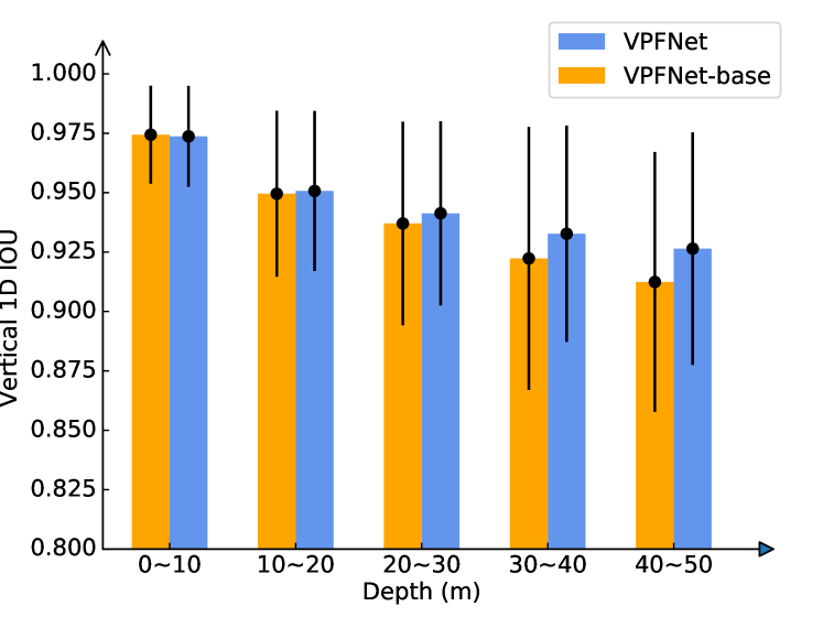
Figure 7: VPFNet can reduce height estimation errors compared to VPFNet-base in all depth ranges, especially for faraway objects. Y-axis is the mean value and variance of 1D IOU between GT 2D boxes and predicted 2D boxes

Impact of Data Augmentation: In Table V, we compare the detection results when we have no cut-n-paste, box cut-n-paste as in [36], as well as our mask cut-n-paste with different $\tau_{2D}$ values. The results show that our mask cut-n-paste augmentation leads to an improvement of 1.25%, 2.61%, and 2.41% for $Easy_{3D}$, $Mod_{3D}$, and $Hard_{3D}$, respectively. Meanwhile, according to Table IV in our paper, the performance improvement brought by our model design is 0.3%, 2.86%, and 2.85% for $Easy_{3D}$, $Mod_{3D}$, and $Hard_{3D}$, respectively. Comparing the two, our model design yields larger improvements than our augmentation scheme on $Mod_{3D}$ and $Hard_{3D}$,.

$N_{x}$	$N_{y}$	$N_{z}$	$N_{layer}$	time(ms)	3D Hard	BEV Hard
30	18	30	6	102	83.25	89.35
25	12	25	6	81	83.24	89.43
25	12	25	1	61	81.20	89.08
16	8	25	6	76	81.11	89.37
16	8	22	6	71	81.16	89.12
16	8	16	6	62	81.03	87.30

TABLE VI: $AP_{3D}$ and inference time with several virtual point density settings (denoted by $N_{x},N_{y},Nz$) and sparse convolution layer number (denoted by $N_{layer}$) in VPFNet. Note that the experiments were conducted on the down-sampled KITTI data, with LiDAR down-sampled to 32 beams.

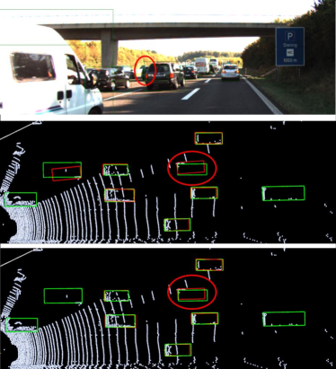
(a) road scenes

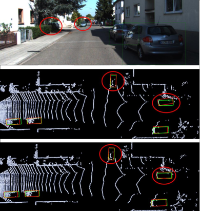
(b) residential scenes

Figure 8: Qualitative results for (a) road scenes and (b) residential scenes. From top to bottom, we have the left image, detection on bird’s eye view from VPFNet-base, and detection on bird’s eye view (BEV) from our proposed VPFNet. Green boxes on the picture mark ground truth boxes while red boxes mark prediction boxes. Predictions with scores $>0.1$ are visualized on the pictures. We highlight some areas in red circle where the BEV detection results are improved significantly.

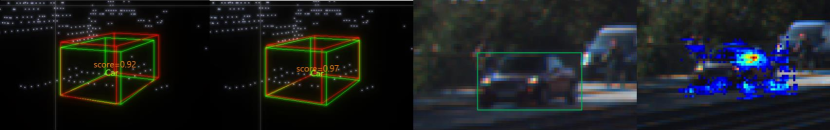
(a) Results for a far-way object. Image features are activated on the top and the wheels of the car.

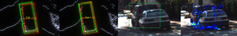
(b) Results for an occluded object. Image features are activated on the bottom of the occluded car.

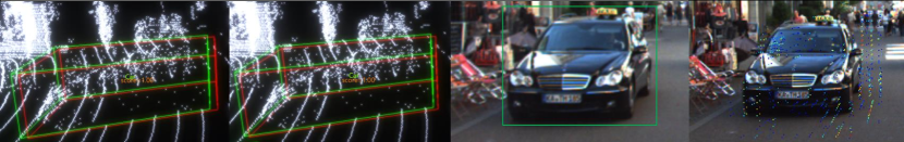
(c) Results for a near object. The box length are improved. We can observe that our sample density is lower than that of the image pixels.

Figure 9: Qualitative results. From left to right: detected object from VPFNet-base, detected object from our VPFNet, the object in left image, the visualization of the intermediate feature vectors ($D_{0}$). Green boxes on the picture mark ground truth boxes while red boxes mark prediction boxes. Predictions with scores $>0.1$ are visualized on the pictures. We show that VPFNet can improve both box size and rotation estimation on near, far, and occluded situations.

V-F Qualitative Results

We also include some quantitative results in Figure 8 and Figure 9, where we visualize the results from VPFNet and VPFNet-base. Figures 8(a)-(b) show that though the box predictions (marked in red) generated by VPFNet-base already have high IoU with the ground truth boxes (marked in green), VPFNet can still improve the accuracy on the bird’s eye view (BEV). Figure 8(a) shows an example in which the rotation estimation of an occluded car is improved. Figure 8(b) shows the rotation estimation of a far-away object and the box size estimation of an occluded box are improved.

Figures 9 (a)-(c) show the results from both detectors, as well as the intermediate feature vectors ($D_{0}$) after sparse convolution. In Figure 9(a), the predicted box height from VPFNet-base exceeds the actual size because LiDAR beams locate only on the middle part of the car. The activated virtual point features are mainly located on the top of the car and the four wheels. In Figure 9(b), the predicted orientation from VPFNet-base shows a drift because the object suffers from a severe occlusion. Figure 9(c) shows that even for near objects, the detection result can be slightly improved by VPFNet.

V-G Inference Time Measurement

In our design, the inference time is mainly affected by the density of virtual points and query points. The submitted version of VPFNet partitions each proposal into $16\times 8\times 22$ grid blocks and $6\times 6\times 6$ query points, resulting in inference time of 63.6 ms and a FPS of 15.7 on a single NVIDIA RTX 2080Ti GPU. Note that there is less than 140 actual LiDAR points located inside of each 3D proposals on average. Table VI shows the overall inference time of VPFNet with different grid block numbers. We observe that although the accuracy increases with the density of virtue points, the latency increases even faster. Therefore it is important to find a trade off between inference time and accuracy.

VI Conclusion

In this work, we present virtual-point fusion to combine LiDAR and stereo data for more accurate 3D object detection. The key difference from existing methods lies in the fact that we take into consideration the resolution mismatch between the two sensors. We employ virtual points whose density is in between that of 3D points and 2D pixels to bridge the resolution gap and to carefully balance data sampling rate and computing efficiency. With virtual points, we can efficiently sample image features while aggregating $K$ nearby point cloud features. Further, final predictions are obtained by having two detection heads with different weights to prevent single-modality dominance. Finally, multi-modal data augmentation techniques are devised to further boost the performance. Experiments on the KITTI dataset prove the effectiveness of the proposed method, which performs the best for several KITTI metrics and supports an FPS of 15.7.

References

- [1] Y. Wang, W.-L. Chao, D. Garg, B. Hariharan, M. Campbell, and K. Q. Weinberger, “Pseudo-lidar from visual depth estimation: Bridging the gap in 3d object detection for autonomous driving,” in Proceedings of the IEEE Conference on Computer Vision and Pattern Recognition, 2019, pp. 8445–8453.
- [2] P. Li, S. Su, and H. Zhao, “RTS3D: real-time stereo 3d detection from 4d feature-consistency embedding space for autonomous driving,” CoRR, vol. abs/2012.15072, 2020.
- [3] Y. Wang, B. Yang, R. Hu, M. Liang, and R. Urtasun, “PLUME: efficient 3d object detection from stereo images,” CoRR, vol. abs/2101.06594, 2021.
- [4] Z. Yang, Y. Sun, S. Liu, and J. Jia, “3dssd: Point-based 3D single stage object detector,” in Proceedings of the IEEE/CVF Conference on Computer Vision and Pattern Recognition, 2020, pp. 11 040–11 048.
- [5] S. Shi, X. Wang, and H. Li, “Pointrcnn: 3d object proposal generation and detection from point cloud,” in Proceedings of the IEEE Conference on Computer Vision and Pattern Recognition, 2019, pp. 770–779.
- [6] A. Geiger, P. Lenz, and R. Urtasun, “Are we ready for autonomous driving? the kitti vision benchmark suite,” in Proceedings of the 2012 IEEE Conference on Computer Vision and Pattern Recognition (CVPR’12), 2012, pp. 3354–3361.
- [7] J. Ku, M. Mozifian, J. Lee, A. Harakeh, and S. L. Waslander, “Joint 3d proposal generation and object detection from view aggregation,” in Proceedings of the 2018 IEEE/RSJ International Conference on Intelligent Robots and Systems (IROS’18). IEEE, 2018, pp. 1–8.
- [8] X. Chen, H. Ma, J. Wan, B. Li, and T. Xia, “Multi-view 3d object detection network for autonomous driving,” in Proceedings of the 2017 IEEE Conference on Computer Vision and Pattern Recognition (CVPR’17), 2017, pp. 1907–1915.
- [9] Z. Wang and K. Jia, “Frustum convnet: Sliding frustums to aggregate local point-wise features for amodal 3d object detection,” arXiv preprint arXiv:1903.01864, 2019.
- [10] C. R. Qi, W. Liu, C. Wu, H. Su, and L. J. Guibas, “Frustum pointnets for 3d object detection from rgb-d data,” in Proceedings of the IEEE conference on computer vision and pattern recognition, 2018, pp. 918–927.
- [11] S. Pang, D. D. Morris, and H. Radha, “Clocs: Camera-lidar object candidates fusion for 3d object detection,” in IEEE/RSJ International Conference on Intelligent Robots and Systems, IROS 2020, Las Vegas, NV, USA, October 24, 2020 - January 24, 2021. IEEE, 2020, pp. 10 386–10 393.
- [12] H. Lu, X. Chen, G. Zhang, Q. Zhou, Y. Ma, and Y. Zhao, “Scanet: Spatial-channel attention network for 3d object detection,” in IEEE International Conference on Acoustics, Speech and Signal Processing, ICASSP 2019, Brighton, United Kingdom, May 12-17, 2019. IEEE, 2019, pp. 1992–1996.
- [13] X. Zhao, Z. Liu, R. Hu, and K. Huang, “3d object detection using scale invariant and feature reweighting networks,” in The Thirty-Third AAAI Conference on Artificial Intelligence, AAAI 2019, The Thirty-First Innovative Applications of Artificial Intelligence Conference, IAAI 2019, The Ninth AAAI Symposium on Educational Advances in Artificial Intelligence, EAAI 2019, Honolulu, Hawaii, USA, January 27 - February 1, 2019. AAAI Press, 2019, pp. 9267–9274.
- [14] J. H. Yoo, Y. Kim, J. S. Kim, and J. W. Choi, “3d-cvf: Generating joint camera and lidar features using cross-view spatial feature fusion for 3d object detection,” ECCV, 2020.
- [15] T. Huang, Z. Liu, X. Chen, and X. Bai, “Epnet: Enhancing point features with image semantics for 3d object detection,” ECCV 2020.
- [16] M. Liang, B. Yang, Y. Chen, R. Hu, and R. Urtasun, “Multi-task multi-sensor fusion for 3d object detection,” in Proceedings of the IEEE Conference on Computer Vision and Pattern Recognition, 2019, pp. 7345–7353.
- [17] S. Vora, A. H. Lang, B. Helou, and O. Beijbom, “Pointpainting: Sequential fusion for 3d object detection,” in 2020 IEEE/CVF Conference on Computer Vision and Pattern Recognition, CVPR 2020, Seattle, WA, USA, June 13-19, 2020. IEEE, 2020, pp. 4603–4611.
- [18] M. Liang, B. Yang, S. Wang, and R. Urtasun, “Deep continuous fusion for multi-sensor 3d object detection,” in Proceedings of the the 15th European Conference on Computer Vision (ECCV’18), 2018, pp. 641–656.
- [19] L. Xie, C. Xiang, Z. Yu, G. Xu, Z. Yang, D. Cai, and X. He, “Pi-rcnn: An efficient multi-sensor 3d object detector with point-based attentive cont-conv fusion module,” in Proceedings of the AAAI Conference on Artificial Intelligence, vol. 34, no. 07, 2020, pp. 12 460–12 467.
- [20] V. A. Sindagi, Y. Zhou, and O. Tuzel, “Mvx-net: Multimodal voxelnet for 3d object detection,” in International Conference on Robotics and Automation, ICRA 2019, Montreal, QC, Canada, May 20-24, 2019. IEEE, 2019, pp. 7276–7282.
- [21] Y. Cui, R. Chen, W. Chu, L. Chen, D. Tian, and D. Cao, “Deep learning for image and point cloud fusion in autonomous driving: A review,” CoRR, vol. abs/2004.05224, 2020.
- [22] J. Deng, S. Shi, P. Li, W. Zhou, Y. Zhang, and H. Li, “Voxel R-CNN: towards high performance voxel-based 3d object detection,” CoRR, vol. abs/2012.15712, 2020.
- [23] S. Qiu, S. Anwar, and N. Barnes, “Geometric back-projection network for point cloud classification,” IEEE Transactions on Multimedia, 2021.
- [24] C. Chen, S. Qian, Q. Fang, and C. Xu, “Hapgn: Hierarchical attentive pooling graph network for point cloud segmentation,” IEEE Transactions on Multimedia, 2020.
- [25] H. Liu, Y. Guo, Y. Ma, Y. Lei, and G. Wen, “Semantic context encoding for accurate 3d point cloud segmentation,” IEEE Transactions on Multimedia, 2020.
- [26] Y. Zhou and O. Tuzel, “Voxelnet: End-to-end learning for point cloud based 3d object detection,” in Proceedings of the 2018 IEEE Conference on Computer Vision and Pattern Recognition (CVPR’18), 2018, pp. 4490–4499.
- [27] Y. Yan, Y. Mao, and B. Li, “Second: Sparsely embedded convolutional detection,” Sensors, vol. 18, no. 10, p. 3337, 2018.
- [28] J. Deng, W. Zhou, Y. Zhang, and H. Li, “From multi-view to hollow-3d: Hallucinated hollow-3d r-cnn for 3d object detection,” arXiv:2107.14391, 2021.
- [29] Z. Liu, H. Tang, Y. Lin, and S. Han, “Point-voxel CNN for efficient 3d deep learning,” in Advances in Neural Information Processing Systems 32: Annual Conference on Neural Information Processing Systems 2019, NeurIPS 2019, December 8-14, 2019, Vancouver, BC, Canada, H. M. Wallach, H. Larochelle, A. Beygelzimer, F. d’Alché-Buc, E. B. Fox, and R. Garnett, Eds., 2019, pp. 963–973.
- [30] D. Garg, Y. Wang, B. Hariharan, M. Campbell, K. Q. Weinberger, and W.-L. Chao, “Wasserstein distances for stereo disparity estimation,” arXiv preprint arXiv:2007.03085, 2020.
- [31] Y. You, Y. Wang, W.-L. Chao, D. Garg, G. Pleiss, B. Hariharan, M. Campbell, and K. Q. Weinberger, “Pseudo-lidar++: Accurate depth for 3d object detection in autonomous driving,” in International Conference on Learning Representations, 2020.
- [32] C. Li, J. Ku, and S. L. Waslander, “Confidence guided stereo 3d object detection with split depth estimation,” arXiv preprint arXiv:2003.05505, 2020.
- [33] Y. Wang, Q. Mao, H. Zhu, Y. Zhang, J. Ji, and Y. Zhang, “Multi-modal 3d object detection in autonomous driving: a survey,” CoRR, vol. abs/2106.12735, 2021. [Online]. Available: https://arxiv.org/abs/2106.12735
- [34] C. R. Qi, H. Su, K. Mo, and L. J. Guibas, “Pointnet: Deep learning on point sets for 3d classification and segmentation,” in Proceedings of the 2017 IEEE Conference on Computer Vision and Pattern Recognition (CVPR’17), 2017, pp. 77–85.
- [35] S. Shi, C. Guo, L. Jiang, Z. Wang, J. Shi, X. Wang, and H. Li, “Pv-rcnn: Point-voxel feature set abstraction for 3d object detection,” in CVPR, 2020.
- [36] C. Wang, C. Ma, M. Zhu, and X. Yang, “Pointaugmenting: Cross-modal augmentation for 3d object detection,” in Proceedings of the IEEE/CVF Conference on Computer Vision and Pattern Recognition, 2021, pp. 11 794–11 803.
- [37] S. Yun, D. Han, S. J. Oh, S. Chun, J. Choe, and Y. Yoo, “Cutmix: Regularization strategy to train strong classifiers with localizable features,” in Proceedings of the IEEE/CVF International Conference on Computer Vision, 2019, pp. 6023–6032.
- [38] Y. Chen, S. Liu, X. Shen, and J. Jia, “Dsgn: Deep stereo geometry network for 3d object detection,” in Proceedings of the IEEE/CVF Conference on Computer Vision and Pattern Recognition, 2020, pp. 12 536–12 545.
- [39] W. Wang, D. Tran, and M. Feiszli, “What makes training multi-modal classification networks hard?” in 2020 IEEE/CVF Conference on Computer Vision and Pattern Recognition, CVPR 2020, Seattle, WA, USA, June 13-19, 2020. IEEE, 2020, pp. 12 692–12 702.
- [40] H. W. Kuhn, “The hungarian method for the assignment problem,” in 50 Years of Integer Programming 1958-2008 - From the Early Years to the State-of-the-Art, M. Jünger, T. M. Liebling, D. Naddef, G. L. Nemhauser, W. R. Pulleyblank, G. Reinelt, G. Rinaldi, and L. A. Wolsey, Eds. Springer, 2010, pp. 29–47.
- [41] A. H. Lang, S. Vora, H. Caesar, L. Zhou, J. Yang, and O. Beijbom, “Pointpillars: Fast encoders for object detection from point clouds,” in Proceedings of the IEEE Conference on Computer Vision and Pattern Recognition, 2019, pp. 12 697–12 705.
- [42] Z. Liu, X. Zhao, T. Huang, R. Hu, Y. Zhou, and X. Bai, “Tanet: Robust 3d object detection from point clouds with triple attention,” arXiv preprint arXiv:1912.05163, 2019.
- [43] L. Du, X. Ye, X. Tan, J. Feng, Z. Xu, E. Ding, and S. Wen, “Associate-3ddet: perceptual-to-conceptual association for 3d point cloud object detection,” in Proceedings of the IEEE/CVF conference on computer vision and pattern recognition, 2020, pp. 13 329–13 338.
- [44] Q. Chen, L. Sun, Z. Wang, K. Jia, and A. Yuille, “Object as hotspots: An anchor-free 3d object detection approach via firing of hotspots,” in European Conference on Computer Vision. Springer, 2020, pp. 68–84.
- [45] W. Shi and R. Rajkumar, “Point-gnn: Graph neural network for 3d object detection in a point cloud,” in Proceedings of the IEEE/CVF conference on computer vision and pattern recognition, 2020, pp. 1711–1719.
- [46] C. He, H. Zeng, J. Huang, X. Hua, and L. Zhang, “Structure aware single-stage 3d object detection from point cloud,” in 2020 IEEE/CVF Conference on Computer Vision and Pattern Recognition, CVPR 2020, Seattle, WA, USA, June 13-19, 2020. IEEE, 2020, pp. 11 870–11 879.
- [47] W. Zheng, W. Tang, S. Chen, L. Jiang, and C.-W. Fu, “Cia-ssd: Confident iou-aware single-stage object detector from point cloud,” arXiv preprint arXiv:2012.03015, 2020.
- [48] W. Zheng, W. Tang, L. Jiang, and C.-W. Fu, “Se-ssd: Self-ensembling single-stage object detector from point cloud,” arXiv preprint arXiv:2104.09804, 2021.
- [49] D. Zhou, J. Fang, X. Song, C. Guan, J. Yin, Y. Dai, and R. Yang, “Iou loss for 2d/3d object detection,” in 2019 International Conference on 3D Vision (3DV). IEEE, 2019, pp. 85–94.
- [50] Y. Chen, S. Liu, X. Shen, and J. Jia, “Fast point r-cnn,” in Proceedings of the IEEE International Conference on Computer Vision, 2019, pp. 9775–9784.
- [51] S. Shi, Z. Wang, J. Shi, X. Wang, and H. Li, “From points to parts: 3d object detection from point cloud with part-aware and part-aggregation network,” IEEE Transactions on Pattern Analysis and Machine Intelligence, 2020.
- [52] Z. Yang, Y. Sun, S. Liu, X. Shen, and J. Jia, “Std: Sparse-to-dense 3d object detector for point cloud,” in Proceedings of the IEEE/CVF International Conference on Computer Vision, 2019, pp. 1951–1960.
- [53] H. Caesar, V. Bankiti, A. H. Lang, S. Vora, V. E. Liong, Q. Xu, A. Krishnan, Y. Pan, G. Baldan, and O. Beijbom, “nuscenes: A multimodal dataset for autonomous driving,” CoRR, vol. abs/1903.11027, 2019.
- [54] P. Sun, H. Kretzschmar, X. Dotiwalla, A. Chouard, V. Patnaik, P. Tsui, J. Guo, Y. Zhou, Y. Chai, B. Caine, V. Vasudevan, W. Han, J. Ngiam, H. Zhao, A. Timofeev, S. Ettinger, M. Krivokon, A. Gao, A. Joshi, Y. Zhang, J. Shlens, Z. Chen, and D. Anguelov, “Scalability in perception for autonomous driving: Waymo open dataset,” in Proceedings of the IEEE/CVF Conference on Computer Vision and Pattern Recognition (CVPR). IEEE, 2020, pp. 2443–2451.
- [55] L. Qi, L. Jiang, S. Liu, X. Shen, and J. Jia, “Amodal instance segmentation with kins dataset,” in Proceedings of the IEEE/CVF Conference on Computer Vision and Pattern Recognition (CVPR), June 2019.
- [56] A. Simonelli, S. R. Bulo, L. Porzi, M. López-Antequera, and P. Kontschieder, “Disentangling monocular 3d object detection,” in Proceedings of the IEEE International Conference on Computer Vision, 2019, pp. 1991–1999.
- [57] S. Peng, W. Jiang, H. Pi, X. Li, H. Bao, and X. Zhou, “Deep snake for real-time instance segmentation,” in Proceedings of the IEEE/CVF Conference on Computer Vision and Pattern Recognition (CVPR), June 2020.
- [58] T.-Y. Lin, P. Goyal, R. Girshick, K. He, and P. Dollár, “Focal loss for dense object detection,” in Proceedings of the IEEE international conference on computer vision, 2017, pp. 2980–2988.