The gradient flow at higher orders in perturbation theory

Abstract

Various results for higher-order perturbative calculations in the gradient-flow formalism are reviewed, including the gradient-flow beta function and the small-flow-time expansion of the hadronic vacuum polarization and the energy-momentum tensor. In addition, the strategy of regions is outlined in order to obtain systematic expansions of gradient-flow integrals, for example at large and small flow times.

1 Introduction

Quantum Chromodynamics (QCD) is a theory with many different facets. So far, quantitative phenomenological results have been obtained mostly in either the strong-coupling regime using lattice regularizations or in the weak-coupling regime where perturbation theory is applicable. Both calculational approaches are highly evolved in themselves. Cross-fertilization is often hindered by the inherently different treatment of ultraviolet divergences in these two calculational approaches.

The gradient-flow formalism (GFF) may provide an excellent opportunity to change this situation. It represents a UV regularization scheme which can be implemented both on the lattice and in perturbation theory. This contribution reviews a number of concrete examples where such a cross-fertilization could be achieved, and where the perturbative calculations have been performed beyond next-to-leading order in perturbation theory. Furthermore, the application of the strategy of regions to gradient-flow integrals is presented, which allows to obtain systematic expansions in dimensionless parameters.

2 The perturbative gradient flow

In the GFF, one defines flowed fields $B^{a}_{\mu}=B^{a}_{\mu}(t)$ and $\chi=\chi(t)$ as solutions of the equations [1, 2] (see also [3, 4])

$$\begin{split}\partial_{t}B^{a}_{\mu}&=\mathcal{D}^{ab}_{\nu}G^{b}_{\nu\mu}+\kappa\mathcal{D}^{ab}_{\mu}\partial_{\nu}B^{b}_{\nu}\,,\\ \partial_{t}\chi&=\Delta\chi-\kappa\partial_{\mu}B^{a}_{\mu}T^{a}\chi\,,\\ \partial_{t}\bar{\chi}&=\bar{\chi}\overleftarrow{\Delta}+\kappa\bar{\chi}\partial_{\mu}B^{a}_{\mu}T^{a}\,.\end{split}$$ (1)

The initial conditions supplementing these differential equations establish the contact to regular QCD:

$$\begin{split}B^{a}_{\mu}(t=0)=A^{a}_{\mu}\,,\qquad\chi(t=0)=\psi\,,\end{split}$$ (2)

where $A^{a}_{\mu}$ and $\psi$ are the regular gluon and quark fields, respectively, and

$$\begin{split}\mathcal{D}^{ab}_{\mu}&=\delta^{ab}\partial_{\mu}-f^{abc}B_{\mu}^{c}\,,\qquad\Delta=(\partial_{\mu}+B^{a}_{\mu}T^{a})(\partial_{\mu}+B^{b}_{\mu}T^{b})\,,\\ G_{\mu\nu}^{a}&=\partial_{\mu}B_{\nu}^{a}-\partial_{\nu}B_{\mu}^{a}+f^{abc}B_{\mu}^{b}B_{\nu}^{c}\,.\end{split}$$ (3)

The arbitrary parameter $\kappa$ will be set equal to one in the following.

Our practical implementation of the GFF in perturbation theory follows the strategy developed in Ref. [5]. It leads to Feynman rules resembling those of regular QCD, but supplemented by flow-time dependent exponentials in the propagators. In addition, the flow equations are reflected through so-called flow lines which couple to the flowed quarks and gluons via flowed vertices. The latter involve integrations over finite intervals of the flow-time variables.

A systematic method how to handle the corresponding Feynman diagrams and integrals through three-loop level has been introduced in Ref. [6]. It is based on qgraf [7] for the generation of Feynman diagrams, FORM [8, 9, 10] for the algebraic manipulation of the resulting amplitudes, Kira+FireFly [11, 12, 13, 14, 15] for the reduction of the Feynman integrals to master integrals, and q2e/exp [16] for interfacing all of these programs. The master integrals can be calculated by following the method outline in Ref. [17], for example.

3 Gluon condensate, quark condensates, and gradient-flow beta function

3.1 Gluon condensate and gradient-flow beta function

The first quantity considered at finite flow time was the gluon condensate in massless QCD [1]. Its perturbative expansion reads

$$\begin{split}&\langle G_{\mu\nu}^{a}(t)G_{\mu\nu}^{a}(t)\rangle=3\frac{\alpha_{s}(\mu)}{\pi t^{2}}\bigg{[}1+\frac{\alpha_{s}(\mu)}{4\pi}\left(e_{10}+4\beta_{0}l_{\mu t}\right)\\ &+\left(\frac{\alpha_{s}(\mu)}{4\pi}\right)^{2}\left(e_{20}+8\left(e_{10}\,\beta_{0}+2\,\beta_{1}\right)l_{\mu t}+16\,\beta_{0}^{2}\,l_{\mu t}^{2}\right)\bigg{]}+\cdots\quad\equiv\quad 3\frac{\bar{\alpha}_{s}(t)}{\pi t^{2}}\,,\end{split}$$ (4)

where $l_{\mu t}\equiv\ln 2\mu^{2}t+\gamma_{\text{E}}$ with Euler’s constant $\gamma_{\text{E}}=0.577\ldots$, and $\alpha_{s}(\mu)$ is the strong coupling in the $\overline{\text{{MS}}}$ scheme which obeys

$$\begin{split}\mu^{2}\frac{\text{d}}{\text{d}\mu^{2}}\frac{\alpha_{s}(\mu)}{\pi}=\beta(\alpha_{s}(\mu))\,,\quad\text{with}\quad\beta(\alpha_{s})=-\sum_{n=0}^{\infty}\left(\frac{\alpha_{s}}{\pi}\right)^{2+n}\beta_{n}\,.\end{split}$$ (5)

In QCD, the first three coefficients of the $\beta$ function in the $\overline{\text{{MS}}}$ scheme read

$$\begin{split}\beta_{0}&=\frac{11}{4}-\frac{n_{f}}{6}\,,\qquad\beta_{1}=\frac{51}{8}-\frac{19}{24}\,n_{f}\,,\\ \beta_{2}&=\frac{2857}{128}-\frac{5033}{1152}\,n_{f}+\frac{325}{3456}\,n_{f}^{2}\approx 22.3-4.37\,n_{f}+0.094\,n_{f}^{2}\,.\end{split}$$ (6)

Setting $t$ to some multiple of $\mu^{2}$, i.e. $t=\mu^{2}/\rho$, acting with $\mu^{2}\text{d}/\text{d}\mu^{2}$ on Eq. 4, and iteratively replacing $\alpha_{s}$ by $\bar{\alpha}_{s}$ according to Eq. 4, one finds the evolution of the gradient-flow coupling:

$$\begin{split}\mu^{2}\frac{\text{d}}{\text{d}\mu^{2}}\frac{\bar{\alpha}_{s}(\mu)}{\pi}=\bar{\beta}(\bar{\alpha}_{s}(\mu))\,,\quad\text{with}\quad\bar{\beta}(\bar{\alpha}_{s})=-\sum_{n=0}^{\infty}\left(\frac{\bar{\alpha}_{s}}{\pi}\right)^{2+n}\bar{\beta}_{n}\,.\end{split}$$ (7)

The first two coefficients are universal, i.e. $\bar{\beta}_{0}=\beta_{0}$ and $\bar{\beta}_{1}=\beta_{1}$, while

$$\begin{split}\bar{\beta}_{2}=\beta_{2}-\frac{1}{4}e_{10}\beta_{1}+\frac{1}{16}\left(e_{20}-e_{10}^{2}\right)\beta_{0}=-59.1-0.536\,n_{f}+0.304\,n_{f}^{2}-0.0030\,n_{f}^{3}\,.\end{split}$$ (8)

Note that the $\rho$-dependence drops out of the $\bar{\beta}$ function. The difference to the $\overline{\text{{MS}}}$ value of Eq. 6 is remarkable. It is illustrated in dependence of $n_{f}$ in Fig. 1 (a). The impact on the QCD $\beta$ function is shown in Fig. 1 (b). One immediately notices that the perturbative convergence is significantly worse in the gradient-flow scheme than in the $\overline{\text{{MS}}}$ scheme (see also Refs. [18, 19, 20, 21]). It would be interesting to understand the source of this behavior in order to allow for a precise independent lattice determination of $\alpha_{s}(M_{Z})$ through the GFF.

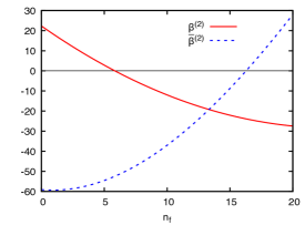
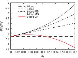
(a)	(b)

Figure 1: (a) Three-loop coefficient of the $\beta$ function in the $\overline{\text{{MS}}}$ (solid-red) and the gradient-flow scheme (dashed-blue). (b) $\beta$ function in the $\overline{\text{{MS}}}$ scheme and the gradient-flow scheme for $n_{f}=0$ ($\mathrm{a}_{s}\equiv\alpha_{s}/\pi$).

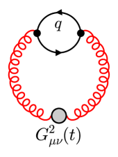
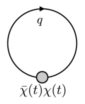
(a)	(b)

Figure 2: Leading-order contributions for the quark mass effects to the gluon and the quark condensate. Diagrams produced with FeynGame [22].

3.2 Quark mass effects

So far, we have considered the case of massless quarks. For the gluon condensate, quark mass effects occur only at next-to-leading order (NLO) through the single Feynman diagram shown in Fig. 2 (a) . They can be taken into account quite easily by using the well-known one-loop expression for the two-point function with external gluons. The result has been expressed in terms of a one-dimensional integral [17]. At higher orders in perturbation theory, approximate results of the mass effects could be obtained using the so-called strategy of regions [23]. To illustrate its application in the GFF, let us consider the simpler case of the quark condensate, where mass effects occur already at leading order (LO), see Fig. 2 (b). The exact mass dependence leads to an incomplete $\Gamma$ function in this case [2]:

$$\begin{split}S(t)\equiv\langle\bar{\chi}(t)\chi(t)\rangle=-\frac{3m}{8\pi^{2}t^{2}}f(m^{2},t)\,,\end{split}$$ (9)

where

$$\begin{split}f(m^{2},t)\equiv t\int_{k}\frac{e^{-tk^{2}}}{k^{2}+m^{2}}=1-m^{2}te^{m^{2}t}\Gamma(0,m^{2}t)\,,\qquad\Gamma(s,x)=\int_{x}^{\infty}\text{d}u\,u^{s-1}e^{-u}\,.\end{split}$$ (10)

Assume that we would like to solve the momentum integral in Eq. 10 as an expansion around $m^{2}\ll 1/t$. Obviously, simply interchanging the expansion with the integration, which corresponds to assuming $k^{2}\gg m^{2}$ in the integrand, leads to IR-divergent integrals:

$$\begin{split}f^{(i)}(m^{2},t)&=t\sum_{n=1}^{\infty}(-m^{2})^{n-1}\int_{k}\frac{e^{-tk^{2}}}{k^{2n}}=\sum_{n=1}^{\infty}(-m^{2})^{n-1}t^{n-1+\epsilon}\frac{\Gamma(D/2-n)}{\Gamma(D/2)}\\ &=1+m^{2}t\left(\frac{1}{\epsilon}+\ln t+1\right)e^{m^{2}t}-(m^{2}t)^{2}-\frac{3}{4}(m^{2}t)^{2}+\ldots\,.\end{split}$$ (11)

On the other hand, considering the region $k^{2}\sim m^{2}$, it follows that $tk^{2}\ll 1$, so we can expand the exponential:

$$\begin{split}f^{(ii)}(m^{2},t)&=t\sum_{n=0}^{\infty}\frac{(-t)^{n}}{n!}\int_{k}\frac{k^{2n}}{k^{2}+m^{2}}=m^{2}t\left[-\frac{1}{\epsilon}-1+\gamma_{\text{E}}+\ln m^{2}\right]e^{m^{2}t}\,.\end{split}$$ (12)

We recall that, despite the fact that the expansion of the integrand is justified only in the respective region, the momentum integral can be taken over all values of $k$, because all complementary regions will combine to scale-less integrals which are discarded in dimensional regularization. Combining the two regions, the $1/\epsilon$ pole cancels and one finds

$$\begin{split}f(m^{2},t)&\stackrel{{\scriptstyle m^{2}\ll 1/t}}{{\rightsquigarrow}}f^{(i)}(m^{2},t)+f^{(ii)}(m^{2},t)=\\ &=1+m^{2}t\,e^{m^{2}t}\,(\ln m^{2}t+\gamma_{\text{E}})-(m^{2}t)^{2}-\frac{3}{4}(m^{2}t)^{3}+{\cal O}((m^{2}t)^{4})\,,\end{split}$$ (13)

which agrees with the asymptotic expansion of the explicit expression given in Eq. 10.

Now let us consider the opposite case: $m^{2}\gg 1/t$. We have again two regions, the first one leading to

$$\begin{split}f(m^{2},t)&\stackrel{{\scriptstyle m^{2}\gg k^{2}}}{{\rightsquigarrow}}\hat{f}^{(i)}(m^{2},t)=t\sum_{n=0}^{\infty}\frac{(-1)^{n}}{m^{2(n+1)}}\int_{k}\,k^{2n}\,e^{-k^{2}t}=\sum_{n=1}^{\infty}(-1)^{n+1}n!\,(m^{2}t)^{-n}\,.\end{split}$$ (14)

The second region is given again by $k^{2}\sim m^{2}$, which means that $k^{2}t\gg 1$. Its contribution vanishes, because the Taylor series of $e^{-1/x}$ around $x=0$ is identical to zero. Therefore,

$$\begin{split}f(m^{2},t)\stackrel{{\scriptstyle m^{2}\gg 1/t}}{{\rightsquigarrow}}=\hat{f}^{(i)}(m^{2},t)=\frac{1}{m^{2}t}-\frac{2}{(m^{2}t)^{2}}+\frac{6}{(m^{2}t)^{3}}+\ldots\end{split}$$ (15)

which again agrees with the Taylor series of Eq. 10 around $1/(m^{2}t)=0$.

Of course, our presentation here is only a sketch of the general idea. At higher orders, one needs to take into account integrations over flow-time parameters. In the small-$t$ limit, all flow-time integration variables are bound to be small as well, and the extension to higher loop order is straightforward. In the large-$t$ limit, however, integration over flow-time parameters extends over “large” and “small” regions, and the expansion of the integrand becomes non-trivial. A general treatment of the strategy of regions for flow-time integrals at higher orders is thus ongoing work and will be presented elsewhere.

4 Hadronic vacuum polarization

Consider the operator product expansion of the correlator of two vector currents $j_{\mu}(x)$ in $n_{f}$-flavor QCD with a single massive quark flavor [24]:

$$\begin{split}\Pi_{\mu\nu}(Q)&\equiv\int\text{d}^{4}x\,e^{iQx}\langle Tj_{\mu}(x)j_{\nu}(0)\rangle=(-\delta_{\mu\nu}+Q_{\mu}Q_{\nu}/Q^{2})\Pi(Q^{2})\\ &\Pi(Q^{2})\stackrel{{\scriptstyle Q^{2}\to\infty}}{{\sim}}C^{(0),\text{{B}}}(Q)+m_{\text{{B}}}^{2}C^{(2),\text{{B}}}(Q)+\sum_{n}C^{\text{{B}}}_{n}(Q)\langle\mathcal{O}_{n}(x=0)\rangle\,,\end{split}$$ (16)

This form reflects the fact that, up to mass dimension two, only the trivial operators $\mathds{1}$ and $m_{\text{{B}}}^{2}\mathds{1}$ contribute, where $m_{\text{{B}}}$ is the bare quark mass. At mass dimension four, one has the following set of physical operators (the space-time argument is suppressed in most of what follows):

$$\begin{split}\mathcal{O}_{1}&=\frac{1}{g_{\text{{B}}}^{2}}F^{a}_{\mu\nu}F^{a}_{\mu\nu}\,,\qquad\mathcal{O}_{2}=\sum_{q=1}^{n_{\text{f}}}\bar{\psi}_{q}\overleftrightarrow{\not{D}}\psi_{q}\,,\qquad\mathcal{O}_{3}=m_{\text{{B}}}^{4}\mathds{1}\,,\end{split}$$ (17)

$$\begin{split}\mbox{where}\qquad F^{a}_{\mu\nu}&=\partial_{\mu}A^{a}_{\nu}-\partial_{\nu}A^{a}_{\mu}+f^{abc}A_{\mu}^{b}A_{\nu}^{c}\,,\qquad\overleftrightarrow{D}\!_{\mu}=\partial_{\mu}-\overleftarrow{\partial}_{\mu}+2A^{a}_{\mu}T^{a}\,.\end{split}$$ (18)

After renormalization of $m_{\text{{B}}}$ and the bare coupling $g_{\text{{B}}}$, the operator matrix elements on the r.h.s. of Eq. 16 are still divergent. The divergences can be absorbed into the bare coefficient functions with the help of operator renormalization:

$$\begin{split}\sum_{n}C_{n}^{\text{{B}}}\mathcal{O}_{n}\equiv\sum_{n}C_{n}Z_{nm}\mathcal{O}_{m}\equiv\sum_{n}C_{n}\mathcal{O}^{\text{{R}}}_{m}\,.\end{split}$$ (19)

The fact that the classical mass dimension of the operators is the same as that of the Lagrangian allows one to express the renormalization matrix $Z$ in terms of the QCD $\beta$ function, the quark mass anomalous dimension, and the anomalous dimension of the vacuum energy to all orders [25].

The operator product expansion of Eq. 16 represents a factorization into long- and short-distance effects. The former are contained in the matrix elements $\langle\mathcal{O}_{n}\rangle$ and their evaluation requires non-perturbative methods such as lattice QCD. The latter are in the coefficient function whose perturbative expressions are known through next-to-next-to-leading order (NNLO) and beyond (see Refs. [26, 27, 28], for example). A precise prediction of $\Pi_{\mu\nu}(Q)$ requires full control of the matching between the two, which is notoriously difficult due to the different regularization and renormalization schemes.

The small-flow-time expansion (SFTX) provides a potential solution to this problem by unifying the renormalization scheme for both the coefficient functions and the operators [5]. The spectrum of possible applications is enormous (see Refs. [29, 30, 31, 32, 33, 34, 35, 36], for example). The idea is to define flowed operators $\tilde{\mathcal{O}}_{n}(t)$ by replacing the regular by flowed fields in Eq. 17, and then expressing them in terms of regular operators in the limit $t\to 0$:

$$\begin{split}\tilde{\mathcal{O}}_{n}(t)&\asymp\zeta_{n}^{(0),\text{{B}}}(t)+\zeta_{n}^{(2),\text{{B}}}(t)m_{\text{{B}}}^{2}+\sum_{m}\zeta^{\text{{B}}}_{nm}(t)\mathcal{O}_{m}=\zeta_{n}^{(0)}(t)+\zeta_{n}^{(2)}(t)m^{2}+\sum_{m,k}\zeta_{nk}(t)\mathcal{O}^{\text{{R}}}_{k}\,.\end{split}$$ (20)

Here, the symbol $\asymp$ denotes that the relation holds only asymptotically for $t\to 0$. The coefficients $\zeta_{n}^{(0)}(t)$, $\zeta_{n}^{(2)}(t)$, and $\zeta_{nm}(t)$ are UV finite. They have been calculated in Ref. [33] through NNLO QCD. While the $\zeta_{nm}(t)$ depend only logarithmically on $t$, $\zeta_{n}^{(0)}(t)$ and $\zeta_{n}^{(2)}(t)$ behave as $1/t^{2}$ and $1/t$ as $t\to 0$. In fact, they simply correspond to the first two terms in the Taylor expansion of the vevs around $m=0$:

$$\begin{split}\zeta_{n}^{(0)}(t)+\zeta_{n}^{(2)}(t)m^{2}=\langle\mathcal{O}_{n}(t)\rangle\Big{|}_{m=0}+m^{2}\frac{d}{dm^{2}}\langle\mathcal{O}_{n}(t)\rangle\Big{|}_{m=0}\,.\end{split}$$ (21)

Inverting Eq. 20 and inserting it into Eq. 16 leads to

$$\begin{split}\Pi(Q)\stackrel{{\scriptstyle Q^{2}\to\infty}}{{\sim}}C^{(0),\text{{B}}}(Q)+m^{2}C^{(2)}(Q)+\sum_{n}\tilde{C}_{n}(t)\bar{\mathcal{O}}_{n}(t)\,,\end{split}$$ (22)

$$\begin{split}\mbox{with}\qquad\tilde{C}_{n}(t)=\sum_{m}C_{m}\zeta^{-1}(t)_{mn}\,,\qquad\bar{\mathcal{O}}_{n}(t)=\tilde{\mathcal{O}}_{n}(t)-\zeta_{n}^{(0)}(t)-m^{2}\zeta_{n}^{(2)}(t)\,.\end{split}$$ (23)

Note that power divergences in the limit $t\to 0$ cancel in the combination $\bar{O}_{n}(t)$. A precise lattice determination of the $\langle\bar{\mathcal{O}}(t)$ could thus open the way towards a novel calculation of the vacuum polarization, and thus independent input for the lattice determination of hadronic contributions to low-energy observables such as the muon anomalous magnetic moment.

5 Energy-momentum tensor

Dropping terms that vanish either under a BRST transformation or by equations of motion, the energy-momentum tensor of QCD takes the form of an operator product expansion similar to Eq. 16:

$$\begin{split}T_{\mu\nu}=\sum_{n=1}^{4}C_{n}\mathcal{O}_{n,\mu\nu}\,,\end{split}$$ (24)

$$\begin{split}\mbox{where}\qquad\mathcal{O}_{1,\mu\nu}&=\frac{1}{g_{\text{{B}}}^{2}}G_{\mu\rho}G_{\rho\nu}\,,\qquad\mathcal{O}_{2,\mu\nu}=\frac{\delta_{\mu\nu}}{g_{\text{{B}}}^{2}}G_{\rho\sigma}G_{\rho\sigma}\,,\\ \mathcal{O}_{3}&=\bar{\psi}\left(\gamma_{\mu}\overleftrightarrow{D}_{\nu}+\gamma_{\nu}\overleftrightarrow{D}_{\mu}\right)\psi\,,\qquad\mathcal{O}_{4}=\delta_{\mu\nu}m_{\text{{B}}}\bar{\psi}\psi\,.\end{split}$$ (25)

However, as opposed to Eq. 16, the “Wilson coefficients” $C_{n}$ in this case are given by simple numerical constants to all orders in perturbation theory:

$$\begin{split}C_{1}=1\,,\qquad C_{2}=-\frac{1}{4}\,,\qquad C_{3}=\frac{1}{4}\,,\qquad C_{4}=0\,.\end{split}$$ (26)

Furthermore, due to the Ward-Takahashi identities among the $Z_{nm}$, the energy-momentum tensor is finite, in the sense that the coefficients $C_{n}$ are not renormalized, i.e. $C_{n}=C_{n}^{\text{{B}}}$.

Using the SFTX, we write the operators as

$$\begin{split}\mathcal{O}_{n}\asymp\sum_{m=1}^{4}\zeta^{\text{{B}},-1}(t)_{nm}\tilde{\mathcal{O}}_{m}(t)\end{split}$$ (27)

and insert this into Eq. 24 to obtain [29, 30]

$$\begin{split}T_{\mu\nu}\asymp\sum_{n=1}^{4}c_{n}(t)\tilde{\mathcal{O}}_{n,\mu\nu}(t)\,,\qquad c_{n}(t)=\sum_{m=1}^{4}C_{m}\zeta^{\text{{B}},-1}_{mn}(t)=\sum_{m=1}^{4}C_{m}\zeta^{-1}_{mn}(t)\,.\end{split}$$ (28)

The coefficients $c_{n}(t)$ are finite even without operator renormalization. They have been evaluated through NNLO [29, 30, 37] and used to study thermodynamics of QCD [32, 38, 39, 40, 41].

Acknowledgments.

I would like to thank Aiman El Asad, Janosch Borgulat, Benedikt Gurdon, Stefano Palmisano, Fabian Lange, Tobias Neumann, Paul Mork, Antonio Rago, Joshua Schophoven, and Andrea Shindler for useful and inspiring conversations.

References

- Lüscher [2010] M. Lüscher, JHEP 08, 071 (2010), [Erratum: JHEP 03, 092 (2014)], 1006.4518.
- Lüscher [2013] M. Lüscher, JHEP 04, 123 (2013), 1302.5246.
- Narayanan and Neuberger [2006] R. Narayanan and H. Neuberger, JHEP 03, 064 (2006), hep-th/0601210.
- Lüscher [2010] M. Lüscher, Commun. Math. Phys. 293, 899 (2010), 0907.5491.
- Lüscher and Weisz [2011] M. Lüscher and P. Weisz, JHEP 02, 051 (2011), 1101.0963.
- Artz et al. [2019] J. Artz, R. V. Harlander, F. Lange, T. Neumann, and M. Prausa, JHEP 06, 121 (2019), [Erratum: JHEP 10, 032 (2019)], 1905.00882.
- Nogueira [2006] P. Nogueira, Nucl. Instrum. Meth. A 559, 220 (2006).
- van Ritbergen et al. [1999] T. van Ritbergen, A. Schellekens, and J. Vermaseren, Int. J. Mod. Phys. A 14, 41 (1999), hep-ph/9802376.
- Vermaseren [2000] J. Vermaseren (2000), math-ph/0010025.
- Kuipers et al. [2013] J. Kuipers, T. Ueda, J. Vermaseren, and J. Vollinga, Comput. Phys. Commun. 184, 1453 (2013), 1203.6543.
- Maierhöfer et al. [2018] P. Maierhöfer, J. Usovitsch, and P. Uwer, Comput. Phys. Commun. 230, 99 (2018), 1705.05610.
- Maierhöfer and Usovitsch [2018] P. Maierhöfer and J. Usovitsch (2018), 1812.01491.
- Klappert and Lange [2020] J. Klappert and F. Lange, Comput. Phys. Commun. 247, 106951 (2020), 1904.00009.
- Klappert et al. [2021a] J. Klappert, S. Y. Klein, and F. Lange, Comput. Phys. Commun. 264, 107968 (2021a), 2004.01463.
- Klappert et al. [2021b] J. Klappert, F. Lange, P. Maierhöfer, and J. Usovitsch, Comput. Phys. Commun. 266, 108024 (2021b), 2008.06494.
- Harlander et al. [1998] R. Harlander, T. Seidensticker, and M. Steinhauser, Phys. Lett. B 426, 125 (1998), hep-ph/9712228.
- Harlander and Neumann [2016] R. V. Harlander and T. Neumann, JHEP 06, 161 (2016), 1606.03756.
- Dalla Brida and Lüscher [2016] M. Dalla Brida and M. Lüscher, PoS LATTICE2016, 332 (2016), 1612.04955.
- Fodor et al. [2018] Z. Fodor, K. Holland, J. Kuti, D. Nogradi, and C. H. Wong, EPJ Web Conf. 175, 08027 (2018), 1711.04833.
- Dalla Brida and Ramos [2019] M. Dalla Brida and A. Ramos, Eur. Phys. J. C 79, 720 (2019), 1905.05147.
- Peterson et al. [2021] C. T. Peterson, A. Hasenfratz, J. van Sickle, and O. Witzel, in 38th International Symposium on Lattice Field Theory (2021), 2109.09720.
- Harlander et al. [2020a] R. Harlander, S. Klein, and M. Lipp, Comput. Phys. Commun. 256, 107465 (2020a), 2003.00896.
- Beneke and Smirnov [1998] M. Beneke and V. A. Smirnov, Nucl. Phys. B 522, 321 (1998), hep-ph/9711391.
- Dominguez [2014] C. Dominguez, Int. J. Mod. Phys. A 29, 1430069 (2014), 1411.3462.
- Spiridonov and Chetyrkin [1988] V. Spiridonov and K. Chetyrkin, Sov. J. Nucl. Phys. 47, 522 (1988).
- Chetyrkin et al. [1985] K. Chetyrkin, V. Spiridonov, and S. Gorishnii, Phys. Lett. B 160, 149 (1985).
- Chetyrkin et al. [1997] K. Chetyrkin, R. Harlander, J. H. Kühn, and M. Steinhauser, Nucl. Phys. B 503, 339 (1997), hep-ph/9704222.
- Harlander and Steinhauser [1997] R. Harlander and M. Steinhauser, Phys. Rev. D 56, 3980 (1997), hep-ph/9704436.
- Suzuki [2013] H. Suzuki, PTEP 2013, 083B03 (2013), [Erratum: PTEP 2015, 079201 (2015)], 1304.0533.
- Makino and Suzuki [2014] H. Makino and H. Suzuki, PTEP 2014, 063B02 (2014), [Erratum: PTEP 2015, 079202 (2015)], 1403.4772.
- Hieda and Suzuki [2016] K. Hieda and H. Suzuki, Mod. Phys. Lett. A 31, 1650214 (2016), 1606.04193.
- Iritani et al. [2019] T. Iritani, M. Kitazawa, H. Suzuki, and H. Takaura, PTEP 2019, 023B02 (2019), 1812.06444.
- Harlander et al. [2020b] R. V. Harlander, F. Lange, and T. Neumann, JHEP 08, 109 (2020b), 2007.01057.
- Suzuki et al. [2020] A. Suzuki, Y. Taniguchi, H. Suzuki, and K. Kanaya, Phys. Rev. D 102, 034508 (2020), 2006.06999.
- Rizik et al. [2020] M. D. Rizik, C. J. Monahan, and A. Shindler (SymLat), Phys. Rev. D 102, 034509 (2020), 2005.04199.
- Mereghetti et al. [2021] E. Mereghetti, C. J. Monahan, M. D. Rizik, A. Shindler, and P. Stoffer (2021), 2111.11449.
- Harlander et al. [2018] R. V. Harlander, Y. Kluth, and F. Lange, Eur. Phys. J. C 78, 944 (2018), [Erratum: Eur.Phys.J.C 79, 858 (2019)], 1808.09837.
- Kitazawa et al. [2019] M. Kitazawa, S. Mogliacci, I. Kolbé, and W. A. Horowitz, Phys. Rev. D 99, 094507 (2019), 1904.00241.
- Shirogane et al. [2021] M. Shirogane, S. Ejiri, R. Iwami, K. Kanaya, M. Kitazawa, H. Suzuki, Y. Taniguchi, and T. Umeda (WHOT-QCD), PTEP 2021, 013B08 (2021), 2011.10292.
- Yanagihara et al. [2020] R. Yanagihara, M. Kitazawa, M. Asakawa, and T. Hatsuda, Phys. Rev. D 102, 114522 (2020), 2010.13465.
- Taniguchi et al. [2020] Y. Taniguchi, S. Ejiri, K. Kanaya, M. Kitazawa, H. Suzuki, and T. Umeda (WHOT-QCD), Phys. Rev. D 102, 014510 (2020), [Erratum: Phys.Rev.D 102, 059903 (2020)], 2005.00251.