First Power Linear Unit with Sign

Abstract

Convolutional neural networks (CNNs) have shown great dominance in vision tasks because of their tremendous capability to extract features from visual patterns, in which activation units serve as crucial elements for the entire structure, introducing non-linearity to the data processing systematically. This paper proposes a novel and insightful activation method termed FPLUS, which exploits mathematical power function with polar signs in form. It is enlightened by common inverse operation while endowed with an intuitive meaning of bionics. The formulation is derived theoretically under conditions of some prior knowledge and anticipative properties, and then its feasibility is verified through a series of experiments using typical benchmark datasets, whose results indicate our approach owns superior competitiveness among numerous activation functions, as well as compatible stability across many CNN architectures. Furthermore, we extend the function presented to a more generalized type called PFPLUS with two parameters that can be fixed or learnable, so as to augment its expressive capacity, and outcomes of identical tests validate this improvement. Therefore we believe the work in this paper has a certain value of enriching the family of activation units.

1 Introduction

As a core component embedded in CNN, the activation unit models the synapse in a way of non-linear mapping, transforming different inputs into valid outputs respectively before transmitting to the next node, and this kind of simulation is partly motivated by neurobiology, such as McCulloch and Pitts’ M-P model [1], Hodgkin and Huxley’s H-H equation [2], Dayan and Abbott’s firing rate curve, etc. As a consequence, a neural network is inherently non-linear owing to the contribution of hidden layers, in which activation function is the source providing such vitally important property. Thus it can be seen that an appropriate setup of non-linear activation should not be neglected for the neural networks, and the option of this module usually varies according to the scenarios and requirements.

Over the years, a variety of activation functions have come into being successively, and some of them attain excellent performance. Sigmoid is applied in the early days but deprecated soon because of the severe gradient vanishing problem, which gets considerable alleviation from ReLU [3, 4]. However, the risk of dying neurons makes ReLU vulnerable and hence a lot of variants like Leaky ReLU [5] try to fix this shortcoming. Subsequently, ELU [6] is proposed to address the bias shift effect while its limitation is relatively settled by supplementary strategies such as SELU [7]. Meanwhile, combinative modality is another way to implement that merges different activation functions, e.g. Swish [8, 9] and Mish [10]. As for works including Maxout [11] and ACON [12], they attempt to unify several methods into the same paradigm. Besides, a few ways approximate the sophisticated function through piecewise linear analog for reduction of complexity, like hard-Swish [13].

What mentioned above presents a sketchy outline of remarkable progress about activation units in recent decades, that most of them are based on the transform, recombination, or amendment of linear and exponential models, sometimes logarithmic, but rarely seen with mathematical power form, and this arouse the curiosity what if activated by a certain power function rather than those familiar ones? Additionally, few of the methods take bionic characteristics into account and lack neurobiological implication, which is weak to symbolize the mechanism behind a neural synapse.

Drawing inspiration from the M-P model [1] and perceptron theory [14], as well as binary connect algorithm [15] and symmetric power activation functions [16], this paper proposes a new approach of activation which considers sign function as the switch factor and applies distinct first power functions to positive and negative input respectively, so a bionic meaning is imparted to it in some degree, and we name it as first power linear unit with sign (FPLUS). In terms of what has been discussed in [17] by Bengio et al., we theoretically derive the subtle representation in form of power function under some designated premises, which are in accordance with the attributes that a reasonable activation unit requires. Furthermore, to follow the spirits of PReLU [18], PELU [19], and other parallel works, we generalize the expression to an adjustable form with two parameters which can be either manually set or learned from the training process, regulating both amplitude and flexure of the function shape, so as to help optimization when fine-tuning, and naturally we call it parametric version (PFPLUS).

Of course, we conduct a sequence of experiments to verify the feasibility and robustness of proposed FPLUS and PFPLUS, also compare them with some popular activation units in classification task to examine how our methods perform, which demonstrates that the approach we come up with is capable of achieving comparable and steady results. Meanwhile, in order to figure out a preferable dynamic scope of fluctuation intervals, we explore the setting influence of two controllable parameters by various initialization or assignment, and a preliminary optimization tendency is obtained.

The main contributions of our work can be briefly summarized as below: (1) we theoretically propose a new activation formulation FPLUS which contains bionic allusion, and extend it to a generalized form PFPLUS with tunable parameters; (2) we carry out experiments diversely to validate the performance of our methods, and the results demonstrate their advantages of competence; (3) effect of parameters’ variation is explored by tests, which analyses the dynamic property of PFPLUS.

The remainder of this paper is divided into five sections as follows. Section 2 reviews some representative activation functions in recent years. Section 3 describes our method’s derivation in detail, while its characteristics and attributes are analyzed in section 4. Section 5 includes experimental results and objective discussion. Eventually, a conclusive summary is presented in section 6.

2 Related Works

As is known to all, there exist a number of activation functions so far, some of which obtain significant breakthroughs. We illustrate part of them and our work FPLUS with corresponding derivatives in Fig. 1, also we list formulae of the prominent ones below.

Conventional activation function sigmoid is utilized in the early stage, but Xavier showed us it tends to result in gradient vanishing phenomenon [20] for it is bounded in positive domain, so does the tanh function. However, LeCun’s article [21] pointed out tanh leads to faster convergence for the network than sigmoid because the former one has zero-mean outputs, which are more in accord with the condition of natural gradient expounded in [22], and thus iteration can be reduced. Nevertheless, both of them produce saturated output when there comes large positive input, making the parameter’s updating probably stagnate.

$$\mathrm{sigmoid}(x)=\frac{1}{1+e^{-x}}$$ (1)

$$\mathrm{tanh}(x)=\frac{e^{x}-e^{-x}}{e^{x}+e^{-x}}$$ (2)

Afterward, ReLU [3, 4] is widely employed as the activation function in CNN. Not only does it have easy shape and concise expression, but also alleviates the problem of gradient diffusion or explosion through identity mapping in positive domain. Still, it forces the output of negative value to be zero, and thereby introduces the distribution of sparsity to the network. Even though this sort of setting seems plausible referring to neurobiological literature [23, 24], it as well brings about the disadvantage called dying neurons, which are the units not activated since their gradients reach zero, and in that case, parameters can’t be updated. Therefore to overcome this drawback, Leaky ReLU [5] assigns a fixed slope of non-zero constant to the negative quadrant. However, the value specified is extremely sensitive, so PReLU [18] makes it trainable, but this way inclines to cause overfitting. Then RReLU [25] changes it to be stochastically sampled from a probability distribution, resembling random noise so that generating regularization. On the other hand, instead of focusing on the activation function itself, some methods seek assistance from auxiliary features distilled additionally, such as antiphase information for CReLU [26], and spatial context for FReLU [27], DY-ReLU [28], but this means more overhead on pretreatment.

$$\mathrm{ReLU}(x)=\begin{dcases}x,&\text{if }x\geqslant 0\\ 0,&\text{if }x<0\end{dcases}$$ (3)

$$\mathrm{LReLU}(x)=\begin{dcases}x,&\text{if }x\geqslant 0\\ \alpha x,&\text{if }x<0\end{dcases}\quad(\alpha>0)$$ (4)

In contrast with ReLU, another classic alternative is ELU [6], which replaces the output of negative domain with an exponential function. In this way, ELU avoids the predicament of dead activation from zero derivative, also mitigates the effect of bias shift by pushing the mean of outputs closer to zero. Besides, it appears robust to the noise due to the existence of saturation in negative quadrant. Later CELU [29] remedies its flaw of not maintaining differentiable continuously in some cases, while PELU [19] gives it more flexibility with learnable parameters. In addition, SELU [7] is proved to possess a self-normalizing attribute with respect to the fixed point which is supposed after allocating scale factors, and FELU [30] provides a peculiar perspective to realize speeding-up exponential activation by equivalent transformation.

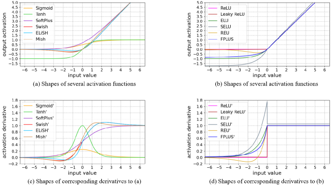
Figure 1: Shapes of typical activation functions and their corresponding derivatives.

$$\mathrm{ELU}(x)=\begin{dcases}x,&\text{if }x\geqslant 0\\ \alpha(e^{x}-1),&\text{if }x<0\end{dcases}\quad(\alpha>0)$$ (5)

$$\mathrm{SELU}(x)=\lambda\cdot\begin{dcases}x,&\text{if }x\geqslant 0\\ \alpha(e^{x}-1),&\text{if }x<0\end{dcases}\\ (\lambda>1,\alpha>0)$$ (6)

Besides, the nested or composite mode can be an innovative scheme to generate new activation functions. SiLU [8] for instance, also known as Swish [9], exactly multiplies the input by sigmoidal weight, and ELiSH [31] makes a little alteration on this basis. GELU [32] adopts a similar operation, regarding the cumulative distribution function of Gaussian distribution as the weight, while Mish [10] combines tanh and SoftPlus [33] before weighting the input. As for REU [34], it directly takes an exponential function to be the multiplier which looks like a hybrid of ReLU and ELU, whereas RSigELU [35] even involves extra sigmoid at the cost of making the expression more complicated.

$$\mathrm{Swish}(x)=x\cdot sigmoid(\beta x)\quad(\beta>0)$$ (7)

$$\mathrm{GELU}(x)=x\cdot\frac{1}{\sqrt{2\pi}}\int_{-\infty}^{x}e^{-\frac{t^{2}}{2}}\mathrm{d}t$$ (8)

$$\mathrm{Mish}(x)=x\cdot tanh[ln(1+e^{x})]$$ (9)

It is likewise noticed that piecewise linear approximation of a curve is usually requested in the mobile devices restricted by computing resources, and thus hard-series fitting was put forward, such as hard-sigmoid [15], hard-Swish [13]. Moreover, some other works like Maxout [11], ACON [12] managed to unify multiple types of activation methods into one single paradigm so that each of them becomes a special case to the whole family, yet this means much more parameters have to be learned to fulfill such kind of adaptive conversion, and hence preprocessing efficiency might be undesired.

3 Proposed Method

In this section, we first explain the motivation of our approach more specifically, and the deduction process is described concretely in the next paragraph.

3.1 Source of Motivation

There is no doubt neurobiology offers probative bionic fundamentals to the design of an imitated neural system, for example, CNN is such a milestone that greatly promotes the advancement of computer vision, and it can be traced back to Hubel and Wiesel’s work [36], whose discovery is an inspiration for the conception of CNN framework. Hence bionics-oriented practice sometimes might be a way to find clues or hints of creation [37], to which lots of documents attach great importance.

M-P model [1] follows the principle of a biological neuron, that there exist excitatory and inhibitory two states depending on the polarity of input type, and a threshold determines whether it is activated or not for the neuron. Based on this essence, primitive perceptron [14] utilizes sign function to produce a binary output of type 0 or 1, representing different activation states, so as to abstract out effective and notable information from features generated by lower-level and pass it on to the deep, albeit this is a roughly primeval means. Another recent research called binary connect [15] inherits the idea alike, not that to cope with output but binarize the weight via 1 and -1, whose purpose is decreasing resource consumption on mobile facilities, and such setup could be reckoned as a similar strategy of regularization.

On the other hand, advancement has witnessed multiple activation methods come into being and evolve consecutively, and plenty of mathematical functions have been employed to act as transfer units in neural networks. Still, in comparison to piecewise linear, exponential, and logarithmic formulae, power type functions seem not much popular with little attention, so they are rarely seen in the field. Under the impact of those famous pioneers, only a few works focus on this sort, e.g., [38] creates a power-based composite function, but appears tangled because it introduces fraction and square root at the same time, while [16] changes the positive representation of ReLU by using a couple of power function and its inverse, which are symmetric to the linear part of ReLU, but it lacks further validation on more datasets and networks.

As a consequence, there are many potentialities we can explore and exploit in power type activation theory, and our work probes into how to construct a refined activation function of this kind with simplicity as well as effectiveness, and pays more attention to the contact with bionic meanings.

3.2 Derivation Process

Obviously, the positive part $y=x$ of ReLU is identical mapping, however, it can be also regarded as $y=x^{1}$, i.e. the output is one power over the input, and this is for positive situation, which reflects the excitatory state of a neuron. Associating with implicit bionic allusion, we ponder the question can we represent the inhibitory state in a contrary way based on a certain power type function, corresponding to the negative part of the same united expression through inverse operation?

As the reverse procedure of positive first power, negative first power is doubtless supposed to be allocated to the opposite position in the formula, which will involve 1 and -1 two constant exponents simultaneously in that case, so a sign function is taken into consideration to play the role of switching between them. Meanwhile, the first-order power is relatively common and simple than those higher-order ones, consuming less computational cost while enabling itself to handle bilateral inputs via two distinct branches.

For more generality, we firstly bring in some coefficients $\alpha$, $\beta$, $\omega$, $\theta$ which are finite real numbers and unequal to zero. Besides we give the definition of our formula $f(x)=\alpha[\omega x+\beta]^{sgn(x)}+\theta$, where sgn$(x)$ is the sign function shown as Eq.(10), while a piecewise form of our expression is given in Eq.(11).

$$\mathrm{sgn}(x)=\begin{dcases}1,&\text{if }x\geqslant 0\\ -1,&\text{if }x<0\end{dcases}$$ (10)

$$f(x)=\begin{dcases}\alpha\omega x+\alpha\beta+\theta,&\text{if }x\geqslant 0\\ \frac{\alpha}{\omega x+\beta}+\theta,&\text{if }x<0\end{dcases}$$ (11)

With reference to the usual characteristics and prior knowledge of those typical activation methods, we design our function $f(x)$ to have such expected properties enumerated as follows:

I.   Defined on the set of real numbers:

$$\left.x\right|_{f(x)=\infty}>0$$

II.  Through the origin of coordinate system:

$$f(0)=0$$

III. Continuous at the demarcation point:

$$\lim\limits_{x\to 0^{+}}f(x)=\lim\limits_{x\to 0^{-}}f(x)=f(0)$$

IV. Differentiable at the demarcation point:

$$\left.\dfrac{\partial f(x)}{\partial x}\right|_{x=0^{+}}=\left.\dfrac{\partial f(x)}{\partial x}\right|_{x=0^{-}}$$

V.  Monotone increasing:

$$\forall x\in\mathbb{R}\ ,\ \dfrac{\partial f(x)}{\partial x}\geqslant 0$$

VI. Convex down:

$$\forall x\in\mathbb{R}\ ,\ \dfrac{\partial^{2}f(x)}{\partial x^{2}}\geqslant 0$$

Condition I requires any value on the set of real numbers ought to be valid as input, but we see there exists trouble when the negative part of $f(x)$ expression achieves infinity since the denominator $\omega x+\beta$ of the fraction isn’t allowed to be zero. As a consequence, considering the piecewise attribute, we can just confine the pole point to the opposite interval and this latent defect can be forever avoided. Assuming that $\exists x_{i}\in(-\infty,0)$ , which makes for

$$\omega x_{i}+\beta=0\implies x_{i}=-\dfrac{\beta}{\omega}$$

To cause a paradox, we need

$$x_{i}>0\implies\dfrac{\beta}{\omega}<0\ \cdot\cdot\cdot\cdot\ \text{\char 172}$$

With regard to condition II, it is clear that point $(0,0)$ of the orthogonal plane coordinate system must be a solution to our activation function, and thus we have

$$f(0)=0\implies\alpha\beta+\theta=0\ \cdot\cdot\cdot\cdot\ \text{\char 173}$$

Condition III calls for continuity, so limits on both sides of the demarcation point must exist, while they equal each other and also the value of that point. Hence we list

$$\left.\begin{gathered}\lim\limits_{x\to 0^{+}}f(x)=\alpha\beta+\theta\\ \lim\limits_{x\to 0^{-}}f(x)=\frac{\alpha}{\beta}+\theta\end{gathered}\right\}\implies\alpha\beta+\theta=\dfrac{\alpha}{\beta}+\theta$$

Because $\alpha,\beta\neq 0$ stated above, it comes out

$$\beta=\pm 1\ \cdot\cdot\cdot\cdot\ \text{\char 174}$$

From formula ② it is known that $f(0)=0$ , and solving these simultaneous equations we can obtain

$$\alpha=\begin{dcases}-\theta,&\text{if }\beta=1\\ \theta,&\text{if }\beta=-1\end{dcases}\ \cdot\cdot\cdot\cdot\ \text{\char 175}$$

As for condition IV, it demands taking the derivatives on both sides of the demarcation point and they should be identical, too. Thereby we get

$$\left.\alpha\omega\right|_{x=0^{+}}=\left.\dfrac{-\alpha\omega}{(\omega x+\beta)^{2}}\right|_{x=0^{-}}\implies\alpha\omega=\dfrac{-\alpha\omega}{\beta^{2}}$$

Since $\alpha,\beta,\omega\neq 0$ as previously mentioned, it turns out

$$\beta=i$$

Now that an outcome of imaginary number $i$ occurs, which disobeys the hypothesis that $\beta$ is a real number, the precondition thus needs to be amended.

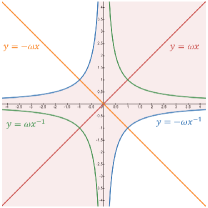
Figure 2: Graphic curves of power functions in a pair of opposite signs with 1 and -1 being exponents. Shadow region signifies a general orientation for $y=\omega x$ to reach tangency with $y=-\omega x^{-1}$.

Observing the graphic curves of a system for the first power functions, sketchily shown as Fig. 2 for example, it can be recognized that line $y=\omega x$ is capable of being tangent to curve $y=-\omega x^{-1}$ somehow, but that will never happen to curve $y=\omega x^{-1}$ because they are always of intersection, and vice versa for line $y=-\omega x$. This fact indicates that the former combination has the potentiality to construct a smooth and derivable function if splicing appropriate portions severally, whereas the latter one does not. The shadow region in the figure implies a possible scope for line $y=\omega x$ to achieve tangency with curve $y=-\omega x^{-1}$, while we can notice it crosses curve $y=\omega x^{-1}$ under any circumstances.

Based on the rules mentioned above, we are aware that for reciprocal types like $y=\omega_{1}x$ and $y=\omega_{2}x^{-1}$, only if the coefficients $\omega_{1}$ and $\omega_{2}$ have contrary signs, can they be differentiable at the demarcation point in piecewise combination when carrying out fundamental functional transformation, such as flip, scaling, translation, etc. Therefore we know

$$\omega_{1}\neq\omega_{2}$$

and the original definition of our function has to be adjusted to

$$f(x)=\begin{dcases}\alpha\omega_{1}x+\alpha\beta+\theta,&\text{if }x\geqslant 0\\ \frac{\alpha}{\omega_{2}x+\beta}+\theta,&\text{if }x<0\end{dcases}$$

where $\alpha,\beta,\omega_{1},\omega_{2},\theta\neq 0$ and all of them are finite real numbers. In this way, we evaluate the differentiability of the boundary point again

$$\left.\alpha\omega_{1}\right|_{x=0^{+}}=\left.\dfrac{-\alpha\omega_{2}}{(\omega_{2}x+\beta)^{2}}\right|_{x=0^{-}}\implies\omega_{1}=\dfrac{-\omega_{2}}{\beta^{2}}$$

Substituting formula ③ into the equation, we are able to figure out the qualitative and quantitative relation

$$\omega_{1}=-\omega_{2}\ \cdot\cdot\cdot\cdot\ \text{\char 176}$$

In the meantime, inequality ① is hence changed into

$$\dfrac{\beta}{\omega_{2}}<0$$

which can be inferred that

$$\omega_{2}\begin{dcases}<0,&\text{if }\beta=1\\ >0,&\text{if }\beta=-1\end{dcases}\ \cdot\cdot\cdot\cdot\ \text{\char 177}$$

As far as condition V is concerned, it involves property of first-order derivative, and owing to the premise that every coefficient is never zero, we accordingly expect

(i) $\ \forall x\geqslant 0,\ \dfrac{\partial f(x)}{\partial x}=\alpha\omega_{1}>0\ \cdot\cdot\cdot\cdot\ \text{\char 178}$

(ii) $\ \forall x<0,\ \dfrac{\partial f(x)}{\partial x}=\dfrac{-\alpha\omega_{2}}{(\omega_{2}x+\beta)^{2}}>0\ \implies\alpha\omega_{2}<0$

Consulting formula ⑤, it is obvious the above two restrictions are equivalent and meeting one of them e.g. inequality ⑦ is quite enough.

Finally, it comes to condition VI, which asks for the function’s being convex down and that refers to second-order derivative, thus we hold

(i) $\forall x\geqslant 0,\ \dfrac{\partial^{2}f(x)}{\partial x^{2}}=0\geqslant 0$

(ii) $\forall x<0,\ \dfrac{\partial^{2}f(x)}{\partial x^{2}}=\dfrac{2\alpha\omega_{2}^{2}}{(\omega_{2}x+\beta)^{3}}>0\implies\dfrac{\alpha}{\omega_{2}x+\beta}>0$

Subordinate condition (i) is apparently self-evident, while for (ii) it can be found out from the formulae ⑤ $\thicksim$ ⑦ that

1. when $\beta=1$, then $\omega_{2}<0,\ \alpha>0\implies\forall x\in(-\infty,0)$ subordinate condition (ii) is tenable

2. when $\beta=-1$, then $\omega_{2}>0,\ \alpha<0\implies\forall x\in(-\infty,0)$ subordinate condition (ii) is tenable

As a result, it means condition VI is inevitable on the basis of previous constraints.

To sum up, any group of real numbers $\alpha,\beta,\omega_{1},\omega_{2},\theta$ which are not equal to zero and satisfy formulae ③ $\thicksim$ ⑦, can be valid coefficients for our function, and we summarize them as two cases.

1. $\beta=1,\ \omega_{2}<0,\ \omega_{1}=-\omega_{2}>0,\ \alpha>0,\ \theta=-\alpha$

2. $\beta=-1,\ \omega_{2}>0,\ \omega_{1}=-\omega_{2}<0,\ \alpha<0,\ \theta=\alpha$

Having case 1 and case 2 substituted into the latest definition of $f(x)$ separately and simplifying them, hence there comes

$$\dagger\text{ case 1: if }\beta=1,\ \text{then }f(x)=\alpha\omega_{1}\cdot\begin{dcases}\ x,&\text{if }x\geqslant 0\\ \dfrac{x}{1-\omega_{1}x},&\text{if }x<0\end{dcases}$$

in which $\alpha>0,\ \omega_{1}>0$;

$$\dagger\text{ case 2: if }\beta=-1,\ \text{then }f(x)=\alpha\omega_{1}\cdot\begin{dcases}\ x,&\text{if }x\geqslant 0\\ \dfrac{x}{1+\omega_{1}x},&\text{if }x<0\end{dcases}$$

in which $\alpha<0,\ \omega_{1}<0$.

Observing the two situations acquired above, it’s not hard to notice that $\alpha\omega_{1}>0$ always stands, and the coefficient of x laying in the denominator of $f(x)$’s piecewise representation within $(-\infty,0)$, is always true to be negative. Therefore we can unify the two cases that $\beta=\pm 1$ for the following new form:

$$f(x)=\lambda\cdot\begin{dcases}\ x,&\text{if }x\geq 0\\ \dfrac{x}{1-\mu x},&\text{if }x<0\end{dcases}\quad(\lambda>0,\mu>0)$$ (12)

Here $\lambda$ is termed as amplitude factor, which controls the degree of saturation for negative zone and the magnitude of slope for positive zone, while $\mu$ is called scale factor, which regulates the speed of attenuation for negative domain only. The derivative of our formulation is given below:

$$f^{\prime}(x)=\lambda\cdot\begin{dcases}\ 1,&\text{if }x\geqslant 0\\ \dfrac{1}{(1-\mu x)^{2}},&\text{if }x<0\end{dcases}\quad(\lambda>0,\mu>0)$$ (13)

So far it can be seen that Eq.(12) is probably the core of our theory, which pretty resembles SELU[7] in conception when taken as a counterpart since they both have linear and decayed areas with two controlled parameters that facilitate their shifting in shapes.

4 Analysis of Characteristics and Attributes

After demonstrating the deduction process of our means and giving the ultimate definition in segmented form, in this section we step further to dig into more traits and properties of it.

In order to merge piecewise activation into one united paradigm for the response, therefore we introduce the Heaviside step function known as Eq.(14), i.e. unit step function, so that enable it to classify the polarity of input’s sign, and react like a switch in neural circuit, transferring the signal with instant gain or gradual suppression.

$$H(x)=\begin{dcases}1,&\text{if }x\geqslant 0\\ 0,&\text{if }x<0\end{dcases}$$ (14)

As long as applying conversion to Eq.(12), we hereby formally set forth parametric first power linear unit with sign (PFPLUS):

$$\mathrm{PFPLUS}(x)=\lambda x\cdot(1-\mu x)^{H(x)-1}$$ (15)

where $H(x)$ is Heaviside step function, and $\lambda,\mu>0$.

Undisputedly, with parameters $\lambda$ and $\mu$ changing, our function proposed will present different shapes in the graph. As shown in Fig. 3, it is similar to ReLU when $\lambda=0.2$ and $\mu=10$, while approximates linear mapping as $\lambda=5$ and $\mu=0.1$. Of course, they can be either learned from training procedure or fixed by initial setting, depending on distinct purpose.

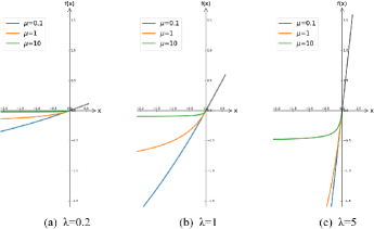
Figure 3: Different shapes of PFPLUS when $\lambda$ and $\mu$ vary.

About trainable PFPLUS in the implementation, we choose established gradient descent as the iterative approach to updating and learning these two coefficients. More than that, we adopt strategies like PReLU [18] to avoid overfitting as much as possible. For every activation layer of PFPLUS, parameters $\lambda$ and $\mu$ are completely identical across all of the channels, in other words, they are channel-shared or channel-wise. As a result for the whole network, the increment of parameters is merely negligible to the total quantity of weights.

Beyond that, Ramachandran et al. have done a lot of work searching for good activation units based on ReLU [39], including unary functions and binary functions. They discovered that those which perform well tend to be concise, often consisting of no more than two elements, and they usually comprise original input, i.e. in the form of $f[x,g(x)]$. The study also perceived that most of them are smooth and equipped with linear regions. However, they missed inquiring into power ones with negative exponents when researching on unary types, whereas our work makes some supplementation in a sense.

Particularly, as the parameters $\lambda$ and $\mu$ are both equal to one, the function becomes a special form like Eq.(16), which is the simplest pattern of its whole family. In addition, considering the views Bengio et al. discussed in [17], we theoretically reckon the advantages for our way as below:

1. For positive zone, identity mapping is retained for the sake of avoiding gradient vanishing problem.

2. For negative zone, as the negative input goes deeper, the outcome will appear a tendency to gradually reach saturation, which offers our method robustness to the noise.

3. Entire outputs’ mean of the unit is close to zero, since the result yielded for negative input isn’t directly zero, but exists a relative minus response to neutralize the holistic activation, so that bias shift effect can be reduced.

4. When having the corresponding formulation of negative part processed in Taylor expansion, seen as Eq.(17) , the operation carried out in negative domain is equivalent to dissociating each order component of the input signal received, and thus more abundant features might be attained up to a point.

5. From an overall perspective, the shape of function is unilateral inhibitive, and this kind of one-sided form could facilitate the introduction of sparsity to output nodes, making them be like logical neurons.

$$f(x)=\begin{dcases}\ x,&\text{if }x\geqslant 0\\ \dfrac{x}{1-x},&\text{if }x<0\end{dcases}$$ (16)

$$\dfrac{x}{1-x}=x+x^{2}+x^{3}+\dots+x^{n-1}+x^{n}+O(x^{n})$$ (17)

Moreover, our method can be further associated with a bionic meaning, as long as we implant sign function listed in Eq.(10) to play the role of neuron switch, and therefrom we officially put forward first power linear unit with sign (FPLUS), shown as Eq.(18).

$$\mathrm{FPLUS}(x)=[\mathrm{sgn}(x)\cdot x+1]^{\mathrm{sgn}(x)}-1$$ (18)

For the two sign functions applied in this definition, the one outside bracket is an exponent for the whole power, and it can be regarded as a discriminant factor to the input’s polarity, while the one inside bracket is a coefficient, which can be seen as a weight to the input, working in a bipolar way somewhat like [15] mentioned.

In conclusion, what expounded above demonstrates our method is in possession of rigorous rationality and adequate novelty. At the same time, there are still numerous other manners we can develop to comprehend its ample connotation.

5 Experiments and Discussion

In this section, we conduct a series of experiments to probe into feasibility, capability, and universality of our method, also validate those inferences we discussed before by classification task, covering controlled trials and ablation study. In order to explore its influence on the performance of extracting features in neural networks, we test it on different CNN architectures across many representative datasets, including MNIST & Fashion-MNIST, Kaggle’s Dogs Vs Cats, Intel Image Classification, and CIFAR-10.

This section is organized by different experiments with each dataset listed above, so it’s divided into 5 main segments.

5.1 Experiments on MNIST & Fashion-MNIST

MNIST is an old but classic dataset created by LeCun et al. in the 1990s, which is made up of handwritten digits $0\sim 9$ with a training set of 60K examples and a test set of 10K examples. These morphologically diverse digits have been self-normalized and centered in grayscale images with $28\times 28$ pixels for each. Similarly, Fashion-MNIST is a popular replacement that emerged in recent years, and it shares the same image size, sample quantity, as well as structure of training and testing splits just like the original MNIST. As the name implies, this dataset is a version of fashion and garments, containing labels from 10 classes.

Seeing there are two mutable factors in our parametric function, we plan to preliminarily explore their effects on the performance of activation as the values vary. To facilitate direct observation of dynamic change and prominent differences, we choose LeNet-5 [40] to learn from the data due to its simplicity and origin.

What comes to the first is an experiment with fixed configurations of $\lambda$ and $\mu$, set with four orders of magnitude for each, which are 0.01, 0.1, 1, and 10. We train the model with MNIST and Fashion-MNIST for 5 epochs separately but follow the same training setups. The batch size is 64 and the learning rate is 0.001, with cross-entropy loss being the loss function and Adam being the optimizer.

Table 1: Training loss and test accuracy on MNIST & Fashion-MNIST.

Dataset	Factor	Loss				Accuracy
		0.01	0.1	1	10	0.01	0.1	1	10
MNIST	0.01	1.573	1.485	1.441	1.534	39.93%	43.85%	44.89%	41.20%
	0.1	0.147	0.114	0.139	0.158	96.21%	97.01%	96.63%	96.05%
	1	0.054	0.046	0.027	0.028	98.40%	98.31%	98.97%	98.92%
	10	0.567	0.430	0.111	0.079	96.21%	96.47%	97.11%	97.45%
Fashion-MNIST	0.01	1.091	1.072	1.065	1.343	52.88%	57.25%	59.45%	52.30%
	0.1	0.630	0.568	0.534	0.579	76.49%	78.84%	79.87%	77.97%
	1	0.309	0.307	0.253	0.267	87.75%	88.18%	89.62%	88.98%
	10	0.496	0.636	0.371	0.341	83.49%	84.99%	86.53%	86.71%

• $\circledcirc$ For each dataset, the best results of loss and accuracy are denoted in blue color.

Table 2: Parameters’ adaptive variation for each activation layer after trained on MNIST.

Initial	Training Loss	Test Accuracy	Learnable Parameters for Each Activation Layer
			Activation1		Activation2		Activation3		Activation4
$\lambda$ and $\mu$			$\lambda_{1}$	$\mu_{1}$	$\lambda_{2}$	$\mu_{2}$	$\lambda_{3}$	$\mu_{3}$	$\lambda_{4}$	$\mu_{4}$
$\lambda,\mu=0.2$	0.003	98.90%	0.8294	0.1312	0.8121	0.4096	0.4798	0.7393	0.3379	0.6136
$\lambda,\mu=0.5$	0.003	99.08%	1.0320	0.7777	0.8125	0.8921	0.5349	1.1050	0.4464	0.7673
$\lambda,\mu=1$	0.002	99.17%	1.1902	1.2234	1.0173	1.2795	0.7196	1.5806	0.6738	1.2830
$\lambda,\mu=2$	0.004	99.00%	1.5427	2.2394	1.0349	2.4056	0.8685	2.4924	0.8976	2.0421
$\lambda,\mu=5$	0.005	98.99%	1.8366	6.0857	1.1883	5.5873	1.1241	5.6929	1.0646	5.9816

Table 3: Parameters’ adaptive variation for each activation layer after trained on Fashion-MNIST.

Initial	Training Loss	Test Accuracy	Learnable Parameters for Each Activation Layer
			Activation1		Activation2		Activation3		Activation4
$\lambda$ and $\mu$			$\lambda_{1}$	$\mu_{1}$	$\lambda_{2}$	$\mu_{2}$	$\lambda_{3}$	$\mu_{3}$	$\lambda_{4}$	$\mu_{4}$
$\lambda,\mu=0.2$	0.109	90.18%	1.3346	0.0297	1.0644	0.6138	0.7340	0.8240	0.3481	1.1056
$\lambda,\mu=0.5$	0.063	90.28%	1.6568	1.0075	1.4744	1.0531	0.9257	1.5719	0.5796	1.5243
$\lambda,\mu=1$	0.044	90.36%	1.6525	1.6226	1.7972	1.1518	1.1746	2.2956	0.8508	2.0996
$\lambda,\mu=2$	0.037	90.02%	1.8306	3.0781	2.1173	1.6818	1.4963	3.3525	1.2920	2.8767
$\lambda,\mu=5$	0.048	89.49%	2.7184	6.6489	2.5286	4.5443	2.3847	6.0374	2.3395	5.4461

The results of training loss and test accuracy on both datasets are listed in Table 1, grouped by different settings of $\lambda$ and $\mu$. Items in blue color are the best outcomes of loss and accuracy relevant to the corresponding configuration of $\lambda$ and $\mu$, which can be seen that our method achieves superior result when the two parameters are equal to 1, getting the lowest loss and highest accuracy than any other combinations for both MNIST and Fashion-MNIST. In addition, factor $\lambda$ seems to be more sensitive than $\mu$ and exhibits a more intense response as the value changes. For each dataset, only considering $\lambda$ with the same $\mu$, results will get better when $\lambda$ grows from 0.01, especially by a large margin for the interval of 0.01 to 0.1, and reaches the optimum around 1, then begins to fall back a little bit. A similar situation happens to $\mu$ basically, but not that conspicuous as the former one. So this study provides us with a tentative scope of proper $\lambda$ and $\mu$ for favorable activation performance, and such regularity implies that an applicable assignment of $\lambda$ and $\mu$ should be neither too large nor too small.

Based on that, we narrow the value range and continue to investigate its preference when $\lambda$ and $\mu$ are capable of being learned dynamically from data. We keep other training setups alike but increase the epoch to 30, and convert our activation function to learnable mode. Because there are just four activation layers in the official structure of LeNet-5, we can easily record the variation tendency for each parameter after learning. More elaborately, we select five grades to start initialization for both $\lambda$ and $\mu$, which are 0.2, 0.5, 1, 2, and 5. Finally, Table 2 and Table 3 give the updated results of two parameters after learning by 30 epochs, and Fig. 4 shows the variation for each activation layer legibly.

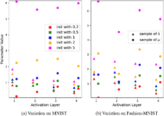
Figure 4: Parameters variation from different initialization on MNIST and Fashion-MNIST after learning. Triangular points are samples of $\lambda$ and circular ones are samples of $\mu$. Initial values are distinguished by different colors.

It can be found that there seems to be some kind of gravity in the vicinity of 1 that attracts $\lambda$ to update along, and those which initialized from both ends, such as 0.2 and 5, tend to evolve towards the central zone. In contrast, $\mu$ appears not much interested in similar renewal but keeps itself fluctuating around the initial value of every layer.

From another perspective, this sort of discrepancy is sensible. Looking back on our PFPLUS formula in Eq.(12), $\lambda$ plays the role of amplitude factor affecting both positive and negative domains. If it is too large, a gradient exploding problem will occur and the capability of resisting noise will be damaged. On the contrary, if it is quite small, the trouble of gradient vanishing will impede the learning process. As for $\mu$, it only manipulates the speed of attenuation for negative domain, and the activation level will decay to saturation sooner or later, which is just a matter of iteration time. So we know $\lambda$ has more impact on the quality of our function compared to $\mu$, but that doesn’t mean the latter one is neglectable since it likewise determines the optimal state of activation performance.

Therefore we see the phenomenon that $\lambda$ inclines to converge on 1 nearby after training, albeit its degree differs in the light of layer, whereas $\mu$ shows no apparent iteration tendency but oscillates around where it is initiated.

5.2 Experiment on Kaggle’s Dogs Vs Cats

Kaggle’s Dogs Vs Cats is an adorable dataset released by Kaggle that contains 25K images in RGB format with arbitrary sizes, and specimens of dogs and cats account for each half. We sample 10% from every category randomly, which has 1250 examples respectively, and then distribute them together to the validation set, so the rest part automatically constitutes the training set.

In the last subsection, we elementarily explore the influence of different specified values on learnable parameters, and this time we change the initialization scheme based on previous work. To extend their variable range, we let the parameters obey some probability distributions rather than give them specific values, which may bring in more flexibility and plasticity.

Besides, we need a deeper network to verify the potentiality of our approach, so we choose the legendary masterpiece ResNet [41] with construction of 34 layers as the framework, of which the activation units are replaced with our PFPLUS initialized in different random distributions. By reason of matching the input size that the network requires, we adjust every image to $224\times 224$ pixels before being fed in. The training epoch is 10 in this experiment with batch size 32, and the learning rate is 0.001 but decays half every two epochs. Customarily, cross-entropy loss is the cost function and Adam is designated as the optimizer.

For comparison, we take the constant distribution of 1 as the baseline, and select uniform distribution as well as normal distribution under conventional, Xavier [20], and Kaiming [18] three ways to experiment. In view of preceding speculation, we empirically test 25 combinations of various distributions, contrasting their training diversification and identifying those good ones. The whole results are placed in the appendix and we excerpt the top-7 best groups to present in Table 4.

Table 4: The top-7 best initialization groups of learnable parameters obeying certain distribution, compared with baseline.

$\lambda$ factor	$\mu$ factor	validation loss	validation accuracy
1	1	0.2885	90.83%
U(0.5, 1.5)	1	0.1923	92.35%
Xavier Normal	1	0.2002	92.35%
Kaiming Normal	1	0.1850	92.11%
1	U(0.5, 1.5)	0.2687	92.35%
1	N(1, $0.1^{2}$)	0.2475	92.51%
N(1, $0.3^{2}$)	N(1, $0.1^{2}$)	0.2271	92.07%
Xavier Uniform	N(1, $0.1^{2}$)	0.1725	92.99%

• $\circledcirc$ $U(a,b)$ means uniform distribution with $a$ and $b$ being lower bound and upper bound.

• $\circledcirc$ $N(\gamma,\sigma^{2})$ means normal distribution with $\gamma$ and $\sigma^{2}$ being mean and variance.

Among all those collocations, we avoid applying Xavier and Kaiming variant distributions to $\mu$, since they will bring about negative initialization that violates the restrictive definition of PFPLUS and fails to make target loss convergent, so Xavier and Kaiming ways are used for $\lambda$ only to make sure the coupled structure of function won’t be jeopardized.

Judging from results of the experiment, we can see it may lead to a better effect if making the parameters subject to a suitable probability distribution, although $\lambda$ and $\mu$ can be both initialized by 1 for the sake of efficiency.

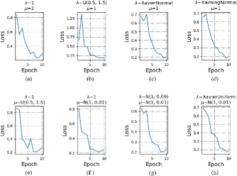
Figure 5: Curves of validation loss for the top-7 best initialization groups and the baseline subject to different distributions.

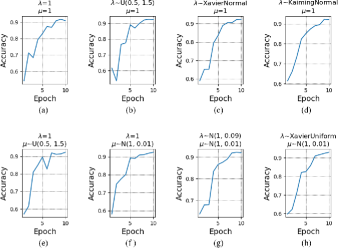
Figure 6: Curves of validation accuracy for the top-7 best initialization groups and the baseline subject to different distributions.

Checking on the entire 25 groups of experimental results, it is noticed that if adopting normal distribution separately, mean of 1 and standard deviation of 0.3 seem to be more reasonable for $\lambda$, whereas standard deviation of 0.1 is better for $\mu$. About uniform distribution, boundaries of 0.5 and 1.5 are good choices for both two parameters.

However, given the overall statistics, we find groups of normal distribution usually achieve higher validation scores than those of uniform distribution, which can be verified through composition proportion of the top 7 best ones as shown in Table 4, dominated by Gaussian type distributions. Besides, under the same circumstances, initialization of Xavier’s version is more recommended to PFPLUS, since it is conducive to the activation that produces zero mean output, while Kaiming’s way principally aims at non-zero centered functions like ReLU.

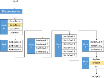
Figure 7: Architecture for traditional ResNet-50 with addition of dropout layer. Details in bottleneck A and B are shown below.

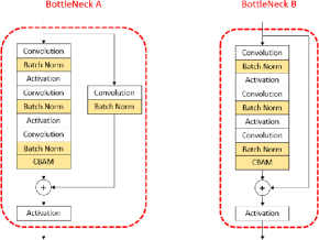
Figure 8: Structures of BottleNeck A and BottleNeck B in Fig. 7’s construction, embedded with CBAM modules specially.

Fig. 5 and Fig. 6 illustrate the validation process and dynamic states of those effective distribution combinations in Table 4, so we can recognize that initialization of $\lambda$ obeying Xavier Uniform distribution while $\mu$ obeying normal distribution with 1 mean and 0.01 variance displays the steadiest loss fall among 8 groups of curves, albeit set of $\lambda$ following Kaiming normal distribution while $\mu$ following constant 1 distribution as well gains eligible performance. As for accuracy, results of (c), (d) and (f), (g), (h) in Fig. 6 show comparatively stable ascending, where constant 1 distribution and Gaussian type distributions involve for many times, so we think of them as preferences to our PFPLUS.

5.3 Experiment on Intel Image Classification Dataset

Intel has ever hosted an image classification challenge and released one scenery dataset, consisting of approximately 17K RGB images of size $150\times 150$ pixels subordinate to 6 categories, which are buildings, forest, glacier, mountain, sea, and street. The dataset splits in training part of 14K examples and test part of 3K, whose ratio is about $82\%:18\%$.

Table 5: Comparison of loss and accuracy for training Intel image classification dataset on ResNet-50 with multiple network configurations, grouped by two ways of learning rate decay.

Architecture Configuration			Step Decay for lr				Exponential Decay for lr
			Testing Loss		Testing Accuracy		Testing Loss		Testing Accuracy
BatchNorm	CBAM	Dropout	ReLU	FPLUS	ReLU	FPLUS	ReLU	FPLUS	ReLU	FPLUS
			0.674	0.484	75.24%	83.18%	1.098	0.822	55.39%	66.95%
$\checkmark$			0.682	0.544	87.28%	88.11%	0.678	0.669	86.21%	86.40%
	$\checkmark$		0.802	0.551	69.98%	80.19%	1.335	1.133	44.25%	55.75%
		$\checkmark$	0.722	0.499	72.57%	82.66%	1.123	0.835	53.19%	67.19%
$\checkmark$	$\checkmark$		0.563	0.571	86.90%	86.71%	0.607	0.609	85.79%	86.31%
$\checkmark$		$\checkmark$	0.846	0.490	87.08%	87.44%	0.683	0.684	86.03%	86.51%
	$\checkmark$	$\checkmark$	0.846	0.617	67.47%	77.53%	1.306	1.151	46.14%	54.58%
$\checkmark$	$\checkmark$	$\checkmark$	0.586	0.496	87.50%	88.50%	0.651	0.666	85.71%	85.75%

• $\circledcirc$ Accuracies in cyan color correspond to the results of trial groups that don’t employ batch normalization layers.

• $\circledcirc$ Check mark $\checkmark$ means relevant module is added in the network.

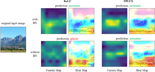
Figure 9: Visualization of feature maps and heat maps produced by model’s final convolutional layer, under two circumstances whether batch normalization is employed or not. Original input image as well as corresponding predictive results for ReLU and FPLUS are given in the figure to check.

As is known to all, the iid condition is substantially a key to resolving the trouble that a training process becomes harder when the network is getting deeper, and this kind of weakness is called bias shift effect [6] or internal covariate shift [42]. Throughout all those reformative activation theories, batch normalization provides such a solution driving inputs of each layer in the network to remain independently and identically distributed.

Taking ReLU [3, 4] as an example, it directly prunes the activation of negative domain for every hidden neuron, making the entire distribution of input data deviates to limit region of the mapping function, so that gradient of lower level in the network probably disappears during backward propagation, and batch normalization exactly serves for dragging it back to a normal distribution with 0 mean and 1 variance.

Nevertheless, unlike ReLU’s bottom truncation, our function FPLUS retains mild activation for negative zone in a gradually saturated way, so as to counteract the shift influence in some degree. Therefore it means ReLU pretty much relies on batch normalization theoretically, while FPLUS remains more tolerable even if without it, affected by less impact than ReLU.

In order to validate the aforementioned hypothesis, we conduct an ablation study in this subsection, mainly researching the influence of batch normalization to non-linear activation, so we compare the responses of ReLU and our FPLUS under two situations whether batch normalization is utilized or not.

As is shown in Fig. 7 and Fig. 8, we opt for ResNet-50 [41] to be the framework, but extra introduce the regularization mechanism dropout [43] and attention module CBAM [44], to explore their mutual effect. Besides, we simultaneously try two attenuation styles for learning rate, including step decay and exponential decay, to investigate which one suits more.

We train the model for 30 epochs with batch size 64 and choose cross-entropy loss like before. The optimizer is SGD with 0.9 being momentum, and the learning rate starts from 0.001, multiplied by 0.1 every 10 epochs in the event of step decay, and making 0.98 the base if it employs exponential decay.

From the results compared in Table 5 we know, on the condition that applying the same decay mode of learning rate, settings with batch normalization are able to produce quite close outcomes for ReLU and FPLUS, while trials with step decay achieve slightly better grades than exponential decay if using identical activation function. On the contrary, if banning batch normalization, both decaying ways for learning rate will generate fallen performance, which is greatly apparent for exponential attenuation. However, our method FPLUS appears more solid and reliable, because it obtains considerably better results than ReLU when they both confront the lack of batch normalization, and this can be seen from the contrast of entries with cyan color in Table 5.

According to the ablation study, separate utilization of dropout or CBAM without batch norm seems to degrade the quality of activation, and such fact manifests the important position of batch norm, which is deemed to lay the foundation for the other two if we want improved performance through combining them.

Fig. 9 shows the different responses of ReLU and FPLUS under two contrastive circumstances whether batch normalization is used or not, and both feature maps and heat maps are given to intuitively illustrate their reactions generated by distinct activation layers.

When the network enables batch normalization, models embedded respectively with ReLU and FPLUS can both output correct prediction, but feature map of ReLU is much more dispersive than that of FPLUS. For heat maps, the response area of FPLUS precisely lies on the key object, whereas ReLU’s does not.

On the other hand, when batch normalization is disabled, models activated by ReLU and FPLUS all produce degenerative feature maps, among which ReLU’s is more ambiguous while that of FPLUS is a little bit better. With regard to heat maps, except for their common flaws at the top, the one belonging to FPLUS concentrates relatively more on valid targets, yet ReLU’s is interfered with by something else in the background. Besides, it’s worth noting that classifier of ReLU misjudges the image category, whereas prediction of FPLUS still hits the right answer.

All things considered, the capacity of batch normalization is absolutely pivotal, on which ReLU relies very much, but our method comparatively shows less dependency and frangibility, notwithstanding it would be better for sure if batch normalization can be exploited at the same time.

5.4 Experiments on CIFAR-10

Table 6: Networks trained on CIFAR-10 and their parameter quantities as well as calculation overhead.

Network	# Params	FLOPs
SqueezeNet [45]	0.735M	0.054G
NASNet [46]	4.239M	0.673G
ResNet-50 [41]	23.521M	1.305G
InceptionV4 [47]	41.158M	7.521G

Table 7: Loss on validation set of CIFAR-10 for each network with different activation functions.

Activation	SqueezeNet	NASNet	ResNet-50	InceptionV4
ReLU	0.350	0.309	0.335	0.442
LReLU	0.345	0.307	0.322	0.412
PReLU	0.365	0.366	0.370	0.305
ELU	0.360	0.280	0.259	0.234
SELU	0.447	0.307	0.295	0.307
FPLUS	0.349	0.287	0.255	0.220
PFPLUS	0.344	0.323	0.251	0.230

• $\circledcirc$ Entries in red color indicate the best results for each network under validation set.

Table 8: Accuracy rate (%) on validation set of CIFAR-10 for each network with different activation functions.

Activation	SqueezeNet	NASNet	ResNet-50	InceptionV4
ReLU	88.67	91.55	91.94	87.95
LReLU	88.63	91.61	92.20	88.18
PReLU	88.91	91.52	92.09	92.95
ELU	87.82	91.70	92.71	92.59
SELU	84.83	90.35	91.10	90.53
FPLUS	88.70	91.46	92.75	93.47
PFPLUS	89.09	91.62	93.13	93.41

• $\circledcirc$ Entries in magenta color indicate the best results for each network under validation set.

Dataset of CIFAR-10 comprises 60K samples with image size of $32\times 32$ pixels in RGB format. It splits into a training set of 50K instances and a validation set of 10K. Training set and validation set have covered each category proportionally for both.

Having discussed the intrinsic values of our formulation in previous experiments, now we plan to explore its compatibility with various network architectures and compare it with other more typical activation functions.

Firstly, we select 4 kinds of networks from lightweight to heavyweight as the foundation frameworks to train on CIFAR-10, and their numbers of parameters as well as the amount of calculation are listed in Table 6. Varieties of activation ways also include ReLU’s improvers LReLU [5] and PReLU [18], as well as ELU [6] and its variant SELU [7].

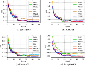
Figure 10: Curves of validating loss for each network applying diverse activation methods.

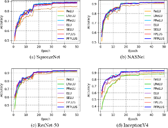
Figure 11: Curves of validating accuracy for each network applying diverse activation methods.

For 4 groups of training, setups of hyperparameters keep the same, and we still use SGD with 0.9 momentum to optimize cross-entropy loss. The iterative epoch is 50 with batch size being 128, and the learning rate starts by 0.01, multiplied by 0.2 every time at 15th, 30th, 40th epoch for decay, which represent the checkpoints of $30\%$, $60\%$ and $80\%$ in training process. For the purpose of data augmentation, we take some measures to transform the training set, such as random cropping, flipping, and rotation.

Loss and accuracy on validation set for each network with distinct activation ways are presented in Table 7 and Table 8, in which colored items stand for the best results of corresponding networks. We can see our method FPLUS and PFPLUS clearly outperform the others on ResNet-50 and InceptionV4, while that is not so evident on SqueezeNet or NASNet.

In addition, we completely record their validating processes of loss and accuracy, as shown in Fig. 10 and Fig. 11. It can be noticed that for heavyweight models like ResNet-50 and InceptionV4, our activation units display swifter loss descending as well as more prominent accuracy rising that enable them to be distinguished from others.

As a consequence, we think our activation function is an effective and reliable approach that is capable of standing the trial, even if confronting a large workload of high intensity such as ImageNet.

Anyway, in comprehensive consideration of the performance on CIFAR-10, we hold that our proposed method shows comparable competitiveness and invariable stability, which make for the promotion of accommodating to as many integrated networks as possible.

6 Conclusion

Taking inspiration from conceptual bionics and inverse operation, this paper proposes a novel and subtle activation method, which involves mathematical first power and switch-like sign function. We theoretically derive the formula under certain specified prior knowledge, and get a concise expression form that owns two adjustable parameters. Either of them regulates the shape of our function, while they can be fixed or learnable. We name our parametric formulation PFPLUS, and FPLUS is one particular case. Furthermore, we investigate the influence of initialization variety for trainable parameters, and find out the limited interval near 1 is a preferable option with interpretability to achieve good performance. Meanwhile, we conduct an ablation study to demonstrate our activation unit is not that vulnerable to the lack of batch normalization, showing less dependency but more robustness. Besides, when compared with other typical activation approaches in the same task, our new way manifests not only appreciable competence but also consistent stability, which provides considerable advantages to its undeniable competitiveness. On the whole, we hold the opinion that our work to some extent enriches the diversity of activation theories.

Appendix A Details for parameter initialization of diverse distributions in Sec. 5.2

Table 1: 25 groups of different initialization for learnable parameters obeying certain distribution, compared with baseline.

No.	$\lambda$ Factor	$\mu$ Factor	Validation Loss	Validation Accuracy
1	1	1	0.2885	90.83%
2	U(0.5, 1.5)	1	0.1923	92.35%
3	U(0.9, 1.1)	1	0.2577	91.31%
4	N(1, $0.3^{2}$)	1	0.2573	91.39%
5	N(1, $0.1^{2}$)	1	0.2944	88.70%
6	XavierUniform	1	0.2012	91.23%
7	XavierNormal	1	0.2002	92.35%
8	KaimingUniform	1	0.2117	91.03%
9	KaimingNormal	1	0.1850	92.11%
10	1	U(0.5, 1.5)	0.2687	92.35%
11	1	U(0.9, 1.1)	0.2535	90.75%
12	1	N(1, $0.3^{2}$)	0.2894	90.83%
13	1	N(1, $0.1^{2}$)	0.2475	92.51%
14	U(0.5, 1.5)	U(0.5, 1.5)	0.2450	91.67%
15	U(0.5, 1.5)	N(1, $0.1^{2}$)	0.2398	91.75%
16	N(1, $0.3^{2}$)	N(1, $0.1^{2}$)	0.2271	92.07%
17	N(1, $0.3^{2}$)	U(0.5, 1.5)	0.2333	91.71%
18	XavierNormal	U(0.5, 1.5)	0.2141	91.55%
19	XavierNormal	N(1, $0.1^{2}$)	0.2080	91.11%
20	XavierUniform	U(0.5, 1.5)	0.2298	90.71%
21	XavierUniform	N(1, $0.1^{2}$)	0.1725	92.99%
22	KaimingNormal	U(0.5, 1.5)	0.2002	91.87%
23	KaimingNormal	N(1, $0.1^{2}$)	0.2506	90.26%
24	KaimingUniform	U(0.5, 1.5)	0.2670	89.46%
25	KaimingUniform	N(1, $0.1^{2}$)	0.3199	88.38%

References

- [1] W. S. Mcculloch, W. Pitts, A logical calculus of the ideas immanent in nervous activity, biol math biophys.
- [2] A. L. Hodgkin, A. F. Huxley, A quantitative description of membrane current and its application to conduction and excitation in nerve., Journal of Physiology 117.
- [3] V. Nair, G. E. Hinton, Rectified linear units improve restricted boltzmann machines, in: Proceedings of the 27th International Conference on International Conference on Machine Learning, ICML’10, Omnipress, Madison, WI, USA, 2010, p. 807–814.
- [4] X. Glorot, A. Bordes, Y. Bengio, Deep sparse rectifier neural networks, in: Proceedings of the 14th International Conference on Artificial Intelligence and Statistics (AISTATS), 2011, pp. 315–323.
- [5] A. L. Maas, A. Y. Hannun, A. Y. Ng, Rectifier nonlinearities improve neural network acoustic models.
- [6] D.-A. Clevert, T. Unterthiner, S. Hochreiter, Fast and accurate deep network learning by exponential linear units (elus), Under Review of ICLR2016 (1997).
- [7] G. Klambauer, T. Unterthiner, A. Mayr, S. Hochreiter, Self-normalizing neural networks.
- [8] S. Elfwing, E. Uchibe, K. Doya, Sigmoid-weighted linear units for neural network function approximation in reinforcement learning, Neural Netw.
- [9] P. Ramachandran, B. Zoph, Q. V. Le, Searching for activation functions.
- [10] D. Misra, Mish: A self regularized non-monotonic neural activation function.
- [11] I. Goodfellow, D. Warde-Farley, M. Mirza, A. Courville, Y. Bengio, Maxout networks, 30th International Conference on Machine Learning, ICML 2013 1302.
- [12] N. Ma, X. Zhang, M. Liu, J. Sun, Activate or not: Learning customized activation, CVPRarXiv:2009.04759.
- [13] A. Howard, M. Sandler, B. Chen, W. Wang, L.-C. Chen, M. Tan, G. Chu, V. Vasudevan, Y. Zhu, R. Pang, H. Adam, Q. Le, Searching for mobilenetv3, in: 2019 IEEE/CVF International Conference on Computer Vision (ICCV), 2019, pp. 1314–1324. doi:10.1109/ICCV.2019.00140.
- [14] Rosenblatt, F., The perceptron: a probabilistic model for information storage and organization in the brain., Psychological Review 65 (1958) 386–408.
- [15] M. Courbariaux, Y. Bengio, J. P. David, Binaryconnect: Training deep neural networks with binary weights during propagations, MIT Press.
- [16] Y. Berradi, Symmetric power activation functions for deep neural networks, in: Proceedings of the International Conference on Learning and Optimization Algorithms: Theory and Applications, 2018, pp. 1–6. doi:10.1145/3230905.3230956.
- [17] C. Gulcehre, M. Moczulski, M. Denil, Y. Bengio, Noisy activation functions, JMLR.org.
- [18] K. He, X. Zhang, S. Ren, J. Sun, Delving deep into rectifiers: Surpassing human-level performance on imagenet classification, CVPR.
- [19] L. Trottier, P. Giguėre, B. Chaib-draa, Parametric exponential linear unit for deep convolutional neural networks, 2017, pp. 207–214. doi:10.1109/ICMLA.2017.00038.
- [20] X. Glorot, Y. Bengio, Understanding the difficulty of training deep feedforward neural networks, Journal of Machine Learning Research 9 (2010) 249–256.
- [21] Y. Lecun, B. Boser, J. Denker, D. Henderson, R. Howard, W. Hubbard, L. Jackel, Backpropagation applied to handwritten zip code recognition, Neural Computation 1 (1989) 541–551. doi:10.1162/neco.1989.1.4.541.
- [22] S. I. Amari, Natural gradient works efficiently in learning, Neural Computation 10 (2).
- [23] D. Attwell, S. B. Laughlin, An energy budget for signaling in the grey matter of the brain, Journal of Cerebral Blood Flow & Metabolism 21 (10) (2001) 1133–1145.
- [24] P. Lennie, The cost of cortical computation, Current biology : CB 13 (2003) 493–7. doi:10.1016/S0960-9822(03)00135-0.
- [25] B. Xu, N. Wang, T. Chen, M. Li, Empirical evaluation of rectified activations in convolutional network.
- [26] W. Shang, K. Sohn, D. Almeida, H. Lee, Understanding and improving convolutional neural networks via concatenated rectified linear units.
- [27] N. Ma, X. Zhang, J. Sun, Funnel activation for visual recognition, ECCVdoi:$10.1007/978-3-030-58621-8_21$.
- [28] Y. Chen, X. Dai, M. Liu, D. Chen, L. Yuan, Z. Liu, Dynamic relu, ECCVdoi:$10.1007/978-3-030-58529-7_21$.
- [29] J. Barron, Continuously differentiable exponential linear units.
- [30] Q. Zheng, D. Tan, F. Wang, Improved convolutional neural network based on fast exponentially linear unit activation function, IEEE Access 7 (2019) 151359–151367.
- [31] M. Basirat, P. M. Roth, The quest for the golden activation function.
- [32] D. Hendrycks, K. Gimpel, Gaussian error linear units (gelus).
- [33] C. Dugas, Y. Bengio, F. Bélisle, C. Nadeau, R. Garcia, Incorporating second-order functional knowledge for better option pricing, in: DBLP, 2001.
- [34] Y. Ying, J. Su, P. Shan, L. Miao, S. Peng, Rectified exponential units for convolutional neural networks, IEEE Access PP (99) (2019) 1–1.
- [35] S. Kiliarslan, M. Celik, Rsigelu: A nonlinear activation function for deep neural networks, Expert Systems with Applications 174 (2) (2021) 114805.
- [36] D. H. Hubel, T. N. Wiesel, Receptive fields of single neurons in the cat’s striate cortex, Journal of Physiology.
- [37] G. S. Bhumbra, Deep learning improved by biological activation functions.
- [38] M. Zhu, W. Min, Q. Wang, S. Zou, X. Chen, Pflu and fpflu: Two novel non-monotonic activation functions in convolutional neural networks, Neurocomputing 429.
- [39] P. Ramachandran, B. Zoph, Q. Le, Swish: a self-gated activation function.
- [40] Y. Lecun, L. Bottou, Gradient-based learning applied to document recognition, Proceedings of the IEEE 86 (11) (1998) 2278–2324.
- [41] K. He, X. Zhang, S. Ren, J. Sun, Deep residual learning for image recognition, 2016 IEEE Conference on Computer Vision and Pattern Recognition (CVPR).
- [42] S. Ioffe, C. Szegedy, Batch normalization: Accelerating deep network training by reducing internal covariate shift.
- [43] N. Srivastava, G. Hinton, A. Krizhevsky, I. Sutskever, R. Salakhutdinov, Dropout: A simple way to prevent neural networks from overfitting, Journal of Machine Learning Research 15 (1) (2014) 1929–1958.
- [44] S. Woo, J. Park, J. Y. Lee, I. S. Kweon, Cbam: Convolutional block attention module, Springer, Cham.
- [45] F. N. Iandola, S. Han, M. W. Moskewicz, K. Ashraf, W. J. Dally, K. Keutzer, Squeezenet: Alexnet-level accuracy with 50x fewer parameters and ¡0.5mb model size.
- [46] B. Zoph, V. Vasudevan, J. Shlens, Q. V. Le, Learning transferable architectures for scalable image recognition.
- [47] C. Szegedy, S. Ioffe, V. Vanhoucke, A. Alemi, Inception-v4, inception-resnet and the impact of residual connections on learning.