Quantum search degeneration under amplitude noise in queries to the oracle

Abstract

We examine how amplitude noise in queries to the oracle degrades a performance of quantum search algorithm. The Grover search and similar techniques are widely used in various quantum algorithms, including cases where rival parties are fighting over confidential data. Hence, the oracle-box wires become the subject of competing activity with an alteration of their normal functioning. Of course, many kinds of errors could arise in this way. Possible influence of dephasing on quantum search was already addressed in the literature. Amplitude damping is another type of errors that should be analyzed first. To study the problem, we introduce a simple model of collective distortions with the use of amplitude damping channel. All the quantities of interest should be considered as functions of the number of Grover’s iterations. In particular, we investigate the success probability with respect to the parameter that characterizes the level of amplitude errors. The success probability degrades significantly even if the error amount is not essential. Namely, this probability soon enough reduces to a value close to one half. We also study trade-off relations between quantum coherence and the success probability in the presence of amplitude noise.

I Introduction

Today, the use of quanta as a tool for information processing has found a great attention wendin17 ; flamini19 ; sage19 ; henriet20 . Although quantum technologies are still in the status of emerging, a stable progress is observed in both theory and practice. Celebrated Shor’s result shor97 gave a stimulus to numerous algorithms for algebraic problems vandam2010 . Grover’s search algorithm grover97 ; grover97a ; grover98 is another fundamental result in quantum information science. Now, the technique of amplitude amplification is one of cornerstones in building quantum algorithms childsQA . The Grover algorithm is optimal for search by means of queries to the oracle bbbv97 ; zalka99 . That is, we invoke the oracle to process any item, whereas the database itself is not exposed explicitly. The original formulation of Grover has later been modified with more general blocks and an arbitrary initial distribution. Various generalizations of quantum search were considered in the literature biham99 ; mardel00 ; biham2002 ; apati2016 ; suzuki21 .

By the oracle, we mean some black box able to calculate values of the desired Boolean function. Any user queries the box by putting concrete values of the argument. In practice, an access to the oracle cannot be treated as exceptional and even reliable. Rather, a number of simultaneous queries will be expected here. Moreover, users’ goals may be different and ever opposite. These are reasons for which errors in the oracle-box wires should be studied. There are various possible scenarios to analyze the above questions. Using simplified model of collective amplitude errors, we address one of such scenarios. In a certain sense, the treatment of rast18 is reformulated with another kind of noise. Another approach to quantum search under localized dephasing was considered in reitzner19 . We also examine the relative entropy of coherence from the viewpoint of its trade-off with the success probability.

This paper is organized in the following way. The preliminary facts are discussed in Sect. II. In Sect. III, we describe and motivate the model of amplitude errors that occur in the oracle-box wires. The built model leads to the recursion equation in terms of the effective Bloch vector. In Sect. IV, we examine changes of the success probability after repeated Grover’s iterations under amplitude noise. It is demonstrated through visualization that the Grover search algorithm is sensitive to errors of the considered type. Using the relative entropy of coherence, we investigate trade-off relations of register coherence with the success probability. In Sect. V, we conclude the paper with a summary of the results. Appendices are devoted to derivation of auxiliary formulas.

II Preliminaries

Let us begin with the original formulation of Grover’s search algorithm. It can be posed as follows. The search space contains $N=2^{n}$ binary strings $x=(x_{1}\cdots{x}_{n})$ with $x_{j}\in\{0,1\}$ so that $x\in\{0,1,\ldots,N-1\}$. The problem is to find one of marked strings that form some set ${\mathcal{M}}$, whereas other strings are all in the complement ${\mathcal{M}}^{{\mathtt{C}}}$. With no loss of generality, one can assume $1\leq|{\mathcal{M}}|\leq{N}/2$. To check the given string $x$, the algorithm appeals to the oracle which returns the value of Boolean function $x\mapsto{F}(x)$ such that $F(x)=1$ for $x\in{\mathcal{M}}$ and $F(x)=0$ for $x\in{\mathcal{M}}^{{\mathtt{C}}}$. The algorithm initializes the $n$-qubit register to $|0\rangle$ and then apply the Hadamard transform, whence the output

$${\mathsf{H}}|0\rangle=\frac{1}{\sqrt{N}}\sum_{x=0}^{N-1}|x\rangle\,.$$ (1)

Superpositions of such a kind are necessary to realize the quantum parallelism deutsch85 . Further, we repeat the Grover iteration involving two steps. The first step with querying the oracle can be represented by the rotation operator

$${\mathsf{J}}=\sum_{x=0}^{N-1}(-1)^{F(x)}\,|x\rangle\langle{x}|\,.$$ (2)

Due to (2), the amplitudes of marked states are multiplied by the factor $\exp({\mathtt{i}}\pi)=-1$. The second step of the Grover iteration leads to the inversion about mean nielsen . It is represented by the operator

$${\mathsf{K}}=2{\mathsf{H}}|0\rangle\langle 0|{\mathsf{H}}-\openone_{N}\,,$$ (3)

where $\openone_{N}$ is the identity operator of the corresponding size. So, the standard Grover iteration is expressed as:

$${\mathsf{G}}={\mathsf{K}}{\mathsf{J}}\,.$$ (4)

In the standard formulation, the initial distribution of amplitudes is taken in the form (1). Then the evolution of amplitudes is described within the two-dimensional picture, for which we use the normalized superpositions of unmarked and marked states, viz.

$$|w\rangle :=\frac{1}{\sqrt{N-M}}\sum_{x\in{\mathcal{M}}^{{\mathtt{C}}}}|x\rangle\,,$$ (5)

$$|m\rangle :=\frac{1}{\sqrt{M}}\sum_{x\in{\mathcal{M}}}|x\rangle\,.$$ (6)

It is useful to put the parameter $\theta\in(0,\pi/2)$ such that $\cos\theta=1-2M/N$ and

$$\sin^{2}\theta/2=\frac{M}{N}\ ,\qquad\cos^{2}\theta/2=1-\frac{M}{N}\ .$$ (7)

Writing operators as matrices in the basis $\bigl{\{}|w\rangle,|m\rangle\bigr{\}}$ results in ${\mathsf{J}}=\mathrm{diag}(+1,-1)=\boldsymbol{\sigma}_{z}$ and

$${\mathsf{K}}=\begin{pmatrix}\cos\theta&\sin\theta\\ \sin\theta&-\cos\theta\end{pmatrix}.$$ (8)

The operator (4) is therefore represented as nielsen :

$${\mathsf{G}}=\begin{pmatrix}\cos\theta&-\sin\theta\\ \sin\theta&\cos\theta\end{pmatrix}.$$ (9)

The initialization state (1) is represented as $\cos(\theta/2)|w\rangle+\sin(\theta/2)|m\rangle$. It is very close to $|w\rangle$ due to smallness of the angle $\theta$ in typical situations. Without noise, each Grover iteration rotates the register state by $\theta$ towards the superposition $|m\rangle$. To characterize a behavior of quantum search under noise, we restrict our consideration to a sufficiently simple model of errors. This choice allows us to answer explicitly basic questions of the study.

Quantum speed-up seems to be impossible without entanglement bpati2002 ; jozsa03 . To analyze quantum algorithms, correlations in register states are considered with respect to few prescribed bases. Hence, the framework to quantify quantum coherence as a potential resource should be developed bcp14 ; plenio16 . The corresponding resource theory allows one to use coherence as a diagnostic tool for quantum chaos anand21 . In algorithms with amplitude amplification, trade-off relations between quantum coherence and the success probability is one of important questions. We shall address this issue in the case, when queries to the oracle are exposed to amplitude noise of the considered type. In general, various approaches to measure quantum correlations were discussed in the literature abc16 ; plenio16 ; hufan16 . Each candidate to quantify the level of coherence is based on some measure to distinguish quantum states. In this paper, the relative entropy of coherence will be used as a quantitative characteristics.

Let us consider the set ${\mathcal{I}}$ of all density matrices of the form:

$$\boldsymbol{\delta}=\sum_{x=0}^{N-1}b(x)\,|x\rangle\langle{x}|\,,\qquad\sum_{x=0}^{N-1}b(x)=1\,.$$ (10)

Such matrices are incoherent in the computational basis. It is further asked how far the given state is from states of the set ${\mathcal{I}}$. The quantum relative entropy of $\boldsymbol{\rho}$ with respect to $\boldsymbol{\omega}$ is defined as vedral02 :

$$D_{1}(\boldsymbol{\rho}||\boldsymbol{\omega}):=\begin{cases}\mathrm{tr}(\boldsymbol{\rho}\ln\boldsymbol{\rho}\,-\boldsymbol{\rho}\ln\boldsymbol{\omega})\,,&\text{if ${\mathrm{ran}}(\boldsymbol{\rho})\subseteq{\mathrm{ran}}(\boldsymbol{\omega})$}\,,\\ +\infty\,,&\text{otherwise}\,.\end{cases}$$ (11)

By ${\mathrm{ran}}(\boldsymbol{\rho})$, one means the range of $\boldsymbol{\rho}$. Using (11), the relative entropy of coherence is introduced as bcp14 :

$$C_{1}(\boldsymbol{\rho}):=\underset{\boldsymbol{\delta}\in{\mathcal{I}}}{\min}\,D_{1}(\boldsymbol{\rho}||\boldsymbol{\delta})\,.$$ (12)

After minimization, we obtain the formula bcp14

$$C_{1}(\boldsymbol{\rho})=S_{1}(\boldsymbol{\rho}_{\mathrm{diag}})-S_{1}(\boldsymbol{\rho})\,,$$ (13)

where $S_{1}(\boldsymbol{\rho})=-\,\mathrm{tr}(\boldsymbol{\rho}\ln\boldsymbol{\rho})$ is the von Neumann entropy of $\boldsymbol{\rho}$. The closest incoherent state is expressed as:

$$\boldsymbol{\rho}_{\mathrm{diag}}:=\sum_{x=0}^{N-1}p(x)\,|x\rangle\langle{x}|\,,\qquad p(x)=\langle{x}|\boldsymbol{\rho}|x\rangle\,.$$

For basic properties of (12), see the papers bcp14 ; plenio16 . Generalized entropic functions are widely used in quantum information science. For this reason, we mark the above quantities by the subscript $1$. Coherence quantifiers induced by quantum divergences of the Tsallis type were examined in rastpra16 . Coherence monotones based on Rényi divergences were considered in chitam2016 ; shao16 ; skwgb16 . Other candidates to quantify the amount of coherence were examined in shao15 ; rpl15 . The geometric coherence is an interesting quantifier of different kind plenio16 . Complementarity relations for quantum coherence were formulated in several ways hall15 ; pati16 ; baietal6 ; rastcomu , including duality between the coherence and path information bera15 ; bagan16 ; bagan20 ; qureshi21 . From the computational viewpoint, the concept of quantum coherence was examined in hillery16 ; hfan2016 . In particular, the authors of hfan2016 reported on coherence depletion in the original Grover algorithm. Relations between coherence and the success probability in generalized amplitude amplification were studied in rastgro17 . Some of these results will be used to analyze Grover’s search in the presence of amplitude errors.

III Collective errors introduced by amplitude damping

There exist many scenarios of decoherence of quantum computations, even if only the oracle-box wires are exposed to noise. Let us consider a model with amplitude damping. Following rast18 , we restrict a consideration to density matrices effectively two-dimensional with respect to the basis $\bigl{\{}|w\rangle,|m\rangle\bigr{\}}$. Such matrices can be represented via the Bloch vector ${\mathbf{r}}=(r_{x},r_{y},r_{z})$, so that

$$\boldsymbol{\rho}=\frac{1}{2}\begin{pmatrix}1+r_{z}&r_{x}-{\mathtt{i}}{r}_{y}\\ r_{x}+{\mathtt{i}}{r}_{y}&1-r_{z}\end{pmatrix}.$$ (14)

With positive parameter $\gamma\leq 1$, we introduce the following Kraus operators:

$${\mathsf{E}}_{0}:=\begin{pmatrix}1&0\\ 0&\sqrt{1-\gamma}\end{pmatrix},\qquad{\mathsf{E}}_{1}:=\begin{pmatrix}0&\sqrt{\gamma}\\ 0&0\end{pmatrix}.$$ (15)

These operators describe the action of amplitude damping $\Phi_{{\mathsf{E}}}$ on density matrices of the considered type. It is easy to see that nielsen

$$(r_{x},r_{y},r_{z})\overset{\Phi_{{\mathsf{E}}}\,}{\longmapsto}\bigl{(}\sqrt{1-\gamma}\,r_{x},\sqrt{1-\gamma}\,r_{y},\gamma+(1-\gamma)r_{z}\bigr{)}\,.$$ (16)

Initializing leads to the density matrix $\boldsymbol{\rho}(0)={\mathsf{H}}|0\rangle\langle 0|{\mathsf{H}}$ with the Bloch vector ${\mathbf{r}}(0)=(\sin\theta,0,\cos\theta)^{\mathsf{T}}$. After $t$ iterations, the success probability is expressed as:

$$P_{\mathrm{suc}}(t)=\langle{m}|\boldsymbol{\rho}(t)|m\rangle=\frac{1-r_{z}(t)}{2}\ .$$ (17)

The following fact is seen from (16) and (17). When $\gamma>0$, the map $\Phi_{{\mathsf{E}}}$ does not alter the success probability only for $r_{z}=1$. The latter corresponds to the superposition $|w\rangle$ of unmarked states.

Let us proceed to the case of noise in the oracle-box wires rast18 . Each iteration acts on density matrices of the register according to the formula:

$$\boldsymbol{\rho}(t)\mapsto\boldsymbol{\rho}(t+1)=\Upsilon_{{\mathsf{K}}}\circ\Phi_{{\mathsf{E}}}\circ\Upsilon_{{\mathsf{J}}}\circ\Phi_{{\mathsf{E}}}\bigl{(}\boldsymbol{\rho}(t)\bigr{)}\,.$$ (18)

The two unitary channels read here as $\Upsilon_{{\mathsf{J}}}(\boldsymbol{\varrho})={\mathsf{J}}\,\boldsymbol{\varrho}\,{\mathsf{J}}^{\dagger}$ and $\Upsilon_{{\mathsf{K}}}(\boldsymbol{\varrho})={\mathsf{K}}\,\boldsymbol{\varrho}\,{\mathsf{K}}^{\dagger}$. For $\gamma=0$, the map $\Phi_{{\mathsf{E}}}$ acts as identical, whence the iteration becomes

$$\boldsymbol{\rho}(t+1)=\Upsilon_{{\mathsf{K}}}\circ\Upsilon_{{\mathsf{J}}}\bigl{(}\boldsymbol{\rho}(t)\bigr{)}={\mathsf{G}}\,\boldsymbol{\rho}(t)\,{\mathsf{G}}^{\dagger}\,.$$ (19)

Applying consequently the map (19) to the initial state (1), we will always deal with pure states of the register. It is not the case for the altered map (18). The above model deals with collective amplitude distortions expressed in the computational basis. This approach allows us to formulate results in a closed analytic form. Also, our scenario does not mean that distortions are similar for all qubits rast18 .

The following method will be used to solve (18). Since only two components of the Bloch vector are non-zero, we further treat ${\mathbf{r}}(t)$ as a column with two entries

$${\mathbf{r}}(t)=\begin{pmatrix}r_{x}(t)\\ r_{z}(t)\end{pmatrix}.$$ (20)

Then the action of operation $\Phi_{{\mathsf{E}}}$ is represented by the formula

$${\mathbf{r}}\overset{\Phi_{{\mathsf{E}}}\,}{\longmapsto}\mathrm{diag}\bigl{(}\sqrt{1-\gamma},1-\gamma\bigr{)}\,{\mathbf{r}}+\gamma\,(0\ 1)^{\mathsf{T}}\,.$$ (21)

We also write

$$2\,{\mathsf{J}}\,\boldsymbol{\rho}\,{\mathsf{J}}^{\dagger}=\boldsymbol{\sigma}_{z}(\openone_{2}+r_{x}\boldsymbol{\sigma}_{x}+r_{z}\boldsymbol{\sigma}_{z})\boldsymbol{\sigma}_{z}=\openone_{2}-r_{x}\boldsymbol{\sigma}_{x}+r_{z}\boldsymbol{\sigma}_{z}\,,$$ (22)

whence the operation $\Upsilon_{{\mathsf{J}}}$ acts on Bloch vectors as the matrix $\mathrm{diag}(-1,+1)$. Due to (8), one has ${\mathsf{K}}\,\openone_{2}\,{\mathsf{K}}^{\dagger}=\openone_{2}$,

$${\mathsf{K}}\,\boldsymbol{\sigma}_{x}{\mathsf{K}}^{\dagger} =-\cos 2\theta\,\boldsymbol{\sigma}_{x}+\sin 2\theta\,\boldsymbol{\sigma}_{z}\,,$$

$${\mathsf{K}}\,\boldsymbol{\sigma}_{z}{\mathsf{K}}^{\dagger} =\sin 2\theta\,\boldsymbol{\sigma}_{x}+\cos 2\theta\,\boldsymbol{\sigma}_{z}\,,$$

so that $r_{x}\mapsto-\cos 2\theta\,r_{x}+\sin 2\theta\,r_{z}$ and $r_{z}\mapsto\sin 2\theta\,r_{x}+\cos 2\theta\,r_{z}$ under the map $\Upsilon_{{\mathsf{K}}}$. Hence, this operation acts on Bloch vectors as the matrix

$$\begin{pmatrix}-\cos 2\theta&\sin 2\theta\\ \sin 2\theta&\cos 2\theta\end{pmatrix}.$$ (23)

Finally, the recursion equation is written in terms of the effective Bloch vector as:

$${\mathbf{r}}(t+1)=\bar{\gamma}\,{\mathsf{L}}\,{\mathbf{r}}(t)+(1-\bar{\gamma}^{2})\begin{pmatrix}\sin 2\theta\\ \cos 2\theta\end{pmatrix},$$ (24)

where $\bar{\gamma}=1-\gamma$ and the matrix ${\mathsf{L}}$ reads as:

$${\mathsf{L}}=\begin{pmatrix}\cos 2\theta&\bar{\gamma}\sin 2\theta\\ -\sin 2\theta&\bar{\gamma}\cos 2\theta\end{pmatrix}.$$ (25)

We further decompose the Bloch vector as:

$${\mathbf{r}}(t)={\mathbf{s}}(t)+(1-\bar{\gamma}^{2})\bigl{(}\openone_{2}-\bar{\gamma}\,{\mathsf{L}}\bigr{)}^{-1}\!\begin{pmatrix}\sin 2\theta\\ \cos 2\theta\end{pmatrix}.$$ (26)

It is possible whenever

$$\det\bigl{(}\openone_{2}-\bar{\gamma}\,{\mathsf{L}}\bigr{)}=1-(\bar{\gamma}+\bar{\gamma}^{2})\cos 2\theta+\bar{\gamma}^{3}\neq 0\,.$$ (27)

It follows from Appendix A that this determinant is strictly positive for $\cos 2\theta<1$ and all $\bar{\gamma}\in[0,1]$. Then the equation (24) leads to

$${\mathbf{s}}(t+1)=\bar{\gamma}\,{\mathsf{L}}\,{\mathbf{s}}(t)\,,\qquad{\mathbf{s}}(t)=\bar{\gamma}^{t}\,{\mathsf{L}}^{t}{\mathbf{s}}(0)\,.$$ (28)

For $\gamma>0$, the vector ${\mathbf{s}}(t)$ becomes zero in the limit $t\to\infty$. Then the Bloch vector coincides with the second term in the right-hand side of (26). This column is explicitly given in (51), whence

$$\lim_{t\to\infty}P_{\mathrm{suc}}(t)=\frac{1}{2}+\frac{(1-\bar{\gamma}^{2})(\bar{\gamma}-\cos 2\theta)}{2\bigl{(}1-(\bar{\gamma}+\bar{\gamma}^{2})\cos 2\theta+\bar{\gamma}^{3}\bigr{)}}\ .$$ (29)

The latter depends on all the parameters $\gamma$, $M$ and $N$. In Appendix B, the components $s_{x}(t)$ and $s_{z}(t)$ are represented in detail. In this way, we express quantities of interest as functions of iterations.

Let us discuss briefly a relevance of the considered noise model to real hardware gates. There are several platforms to obtain quantum processors in the noisy intermediate-scale quantum (NISQ) era preskill18 , e.g., superconducting qubits wendin17 , trapped ions sage19 , neutral atoms henriet20 . Overall, for single-qubit operations high efficiencies can be reached within all these technologies. However, the question of characterization of NISQ devices is very complicated due to a wide range of possibilities for sizing, connection topology and gate implementations. Recent analysis of trapped-ion hardware reported the following debroy20 . With growing the number of qubits, a gate fidelity crucially depends on the type of performed algorithms. On average, they are of the same order or even lesser than will be used in examples of the next section. The noise model posed by (24) is effectively two-dimensional, but the qubit register as a whole undergoes collective errors. It turns out that quite low level of errors is required to implement the search process efficiently. The results of debroy20 give a reason in favor of actual partition of register states into blocks with very different dealing. The role of such blocks in quantum search with noise was already emphasized in reitzner19 .

IV On dynamics of the success probability and quantum coherence

In this section, we will use the above model to study Grover’s search under amplitude noise in the oracle-box wires. It is instructive to visualize $P_{\mathrm{suc}}(t)$ as a function of $t$ for several values of the parameters $\gamma$ and $N$. Before that, we shortly discuss some general features of search under amplitude noise of the considered type. In general, the character of functional behavior depends on relations between the actual values of $\gamma$, $M$ and $N$. The formulas (55) and (56) express the components of ${\mathbf{s}}(t)$ via trigonometric functions under the condition (52). The quantities of interest show an oscillating behavior with slowly decreasing amplitudes. We will also assume the most typical situation $M\ll{N}$, whence $\theta\approx 2\sqrt{M/N}$ due to (7). It is advisable to focus on very small $\gamma$, when the actual search process does not deviate essentially from the idealized one. Moreover, a parametric dependence in this case becomes clearer. For $\gamma=0$, each Grover iteration rotates clockwise the Bloch vector by the angle $2\theta$. It follows from (54) that $\varphi=2\theta+O(\gamma^{2})$. For sufficiently small $\gamma$, one can write

$$s_{x}(t) \simeq\bar{\gamma}^{3t/2}\bigl{[}\sin(2t+1)\theta+O(\gamma)\bigr{]}\,,$$ (30)

$$s_{z}(t) \simeq\bar{\gamma}^{3t/2}\bigl{[}\cos(2t+1)\theta+O(\gamma)\bigr{]}\,.$$ (31)

We refrain from presenting the calculations here. Oscillations of $P_{\mathrm{suc}}(t)$ around its effective mean are determined by (31). What happens with this term, when small $\gamma$ grows at fixed $M$ and $N$? Here, the number of iterations to reach the $k$-th peak of $P_{\mathrm{suc}}(t)$ is such that

$$t_{k}\theta\simeq\frac{(2k-1)\pi}{2}\ ,$$ (32)

whence $\cos(2t_{k}+1)\theta\simeq-\cos\theta$. The following fact is seen from (31). At the given $t$, deviations of $r_{z}(t)$ from its effective mean are mainly defined by $(1-\gamma)^{3t/2}=\exp(-\alpha{t})$ with $\alpha=-(3/2)\ln(1-\gamma)\approx 3\gamma/2$. The number $t_{k}$ remains almost constant, whereas the ratio of deviation amplitudes has a behavior

$$\frac{s_{z}(t_{k})}{s_{z}^{\prime}(t_{k})}\simeq\exp\bigl{\{}(\alpha^{\prime}-\alpha)t_{k}\bigr{\}}\,.$$ (33)

Hence, variations of $P_{\mathrm{suc}}(t)$ are also suppressed with growth of small $\gamma$. This decay is larger for further peaks. The obtained conclusions seem to be quite natural.

The picture is more complicated, when $N$ increases and other parameters are fixed. Due to (32), we write

$$t_{k}\simeq\frac{(2k-1)\pi}{4}\,\sqrt{\frac{N}{M}}\ .$$ (34)

Thus, the number of iterations to reach the $k$-th peak increases proportionally to the square of $N$. Instead of (33), we herewith obtain

$$\frac{s_{z}(t_{k})}{s_{z}^{\prime}(t_{k}^{\prime})}\simeq\exp\!\left\{\frac{(2k-1)\pi\alpha}{4\sqrt{M}}\,\bigl{(}\sqrt{N^{\prime}}-\sqrt{N}\,\bigr{)}\right\}.$$ (35)

For $N^{\prime}>N$, the spread of variations becomes lesser. In other words, the curve of $P_{\mathrm{suc}}(t)$ is stretched with a simultaneous reduce of deviations. Volumizing the search space results in increasing the required iterations jointly with decreasing the actual success probability. This character of changes could be expected without analysis.

Figure 1: The function $P_{\mathrm{suc}}(t)$ for few values of $\gamma$ and $M=2$, with $N=128$ on the left and $N=512$ on the right.

To illustrate the above findings, the quantity $P_{\mathrm{suc}}(t)$ is shown in Fig. 1 for few small values of $\gamma$. The left and right boxes respectively draw the lines for $N=128$ and $N=512$, whereas $M=2$ in both the cases. In accordance with (34), the increase of $N$ by four times implies that the number of peaks on the left is the doubled number of peaks on the right. In addition, consecutive peaks of the success probability decay faster in the right box. We also observe that the limit $t\to\infty$ leads to different values. For fixed $M$, these limiting values depend on both $\gamma$ and $N$ according to (29). For very small $\gamma$, a dependence on $N$ is revealed more brightly. In Fig. 1, we restrict a consideration to $\gamma$ up to five hundredths. Increasing $\gamma$ somewhat further, we have come across a change of functional behavior from trigonometric to hyperbolic type. The formulas (55) and (56) are then replaced with (60) and (61), respectively. In this case, even the first peak of $P_{\mathrm{suc}}(t)$ turns out to be suppressed essentially. Under such circumstances, the search process actually becomes of no effect. Thus, the appearance of amplitude errors even only in the oracle-box wires can lead to devaluation of the quantum search.

The role of quantum coherence in quantum search has found a lot of attention in the literature. It was shown in rastgro17 that

$$h_{1}(P_{\mathrm{suc}})\leq{C}_{1}(\boldsymbol{\rho})+S_{1}(\boldsymbol{\rho})\leq P_{\mathrm{suc}}\,\ln\!\left(\frac{M}{P_{\mathrm{suc}}}\right)+(1-P_{\mathrm{suc}})\,\ln\!\left(\frac{N-M}{1-P_{\mathrm{suc}}}\right),$$ (36)

where $h_{1}(P_{\mathrm{suc}})$ is the binary Shannon entropy. To calculate $C_{1}\bigl{(}\boldsymbol{\rho}(t)\bigr{)}$, we write the actual density matrix as:

$$\boldsymbol{\rho}(t)=\frac{1+r_{z}(t)}{2}\>|w\rangle\langle{w}|+\frac{r_{x}(t)}{2}\,\Bigl{(}|w\rangle\langle{m}|+|m\rangle\langle{w}|\Bigr{)}+\frac{1-r_{z}(t)}{2}\>|m\rangle\langle{m}|\,.$$ (37)

We ask for the diagonal part of $\boldsymbol{\rho}(t)$ in the computation basis. It is represented by the diagonal line, in which the value $\bigl{(}1-P_{\mathrm{suc}}(t)\bigr{)}/(N-M)$ stands $(N-M)$ times and the value $P_{\mathrm{suc}}(t)/M$ stands $M$ times. For $t>0$, the non-zero eigenvalues of $\boldsymbol{\rho}(t)$ read as:

$$\frac{1\pm\|{\mathbf{r}}(t)\|_{2}}{2}\ ,\qquad\|{\mathbf{r}}(t)\|_{2}=\sqrt{r_{x}(t)^{2}+r_{z}(t)^{2}}\leq 1\,.$$ (38)

With the initial distribution (1) we have $\|{\mathbf{r}}(0)\|_{2}=1$. In the considered case of amplitude noise, one has

$$C_{1}\bigl{(}\boldsymbol{\rho}(t)\bigr{)}=P_{\mathrm{suc}}(t)\,\ln\!\left(\frac{M}{P_{\mathrm{suc}}(t)}\right)+\bigl{(}1-P_{\mathrm{suc}}(t)\bigr{)}\ln\!\left(\frac{N-M}{1-P_{\mathrm{suc}}(t)}\right)-S_{1}\bigl{(}\boldsymbol{\rho}(t)\bigr{)}\,.$$ (39)

Here, the upper bound of the right-hand side of (36) is saturated. For the given $P_{\mathrm{suc}}$, this upper bound provides the maximal possible value of $C_{1}(\boldsymbol{\rho})$. We see from (39) a trade-off between $C_{1}\bigl{(}\boldsymbol{\rho}(t)\bigr{)}$ and $P_{\mathrm{suc}}(t)$. When the success probability approaches $1$, the relative entropy of coherence decreases. In the absence of noise, the relative entropy of coherence fluctuates between the maximum and minimum values roughly evaluated as $\ln(N-M)$ and $\ln{M}$. They occur when the success probability is close to its extreme values.

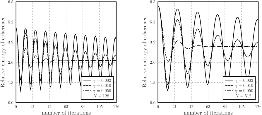
Figure 2: The function $C_{1}\bigl{(}\boldsymbol{\rho}(t)\bigr{)}$ for few values of $\gamma$ and $M=2$, with $N=128$ on the left and $N=512$ on the right.

Amplitude errors lead to suppressing oscillations of all the quantities including the relative entropy of coherence. Of course, the corresponding decay is intensified with growth of $\gamma$. Let us visualize a dependence of the relative entropy of coherence on iterations. Figure 2 shows $C_{1}\bigl{(}\boldsymbol{\rho}(t)\bigr{)}$ under the same circumstances as in Fig. 1. For convenience we note $\ln(N-M)\approx 4.836$ for $N=128$ and $\ln(N-M)\approx 6.234$ for $N=512$. These numbers approximately characterize maximal values for small $\gamma$ and such iterations that oscillation decay has not yet had time to manifest. Minimal values will be close to $\ln 2\approx 0.693$ for vanishing noise. Of course, we again observe all the features mentioned in connection with Fig. 1. In particular, the increase of $N$ by four times results in doubling the period with respect to $t$. Further, consecutive peaks of the relative entropy of coherence are attenuated faster in the right box. Asymptotically, the relative entropy of coherence tends to fit a constant. Then the search process becomes completely degenerated.

V Conclusions

We have examined the case, when queries to the oracle in Grover’s search algorithm are exposed to amplitude error of the specific type. The used model of noise is inspired by the amplitude damping channel reformulated with respect to the two subsets of the unmarked and marked states, respectively. The presented results aim to extend and complete the analysis initiated in the paper rast18 . That paper is devoted to degradation of quantum search under the action of collective phase flips in the oracle-box wires. More general scenarios of quantum search under localized dephasing were examined in reitzner19 . Despite of its simplicity, the used model allows us to probe specific features of search degeneration under amplitude noise in queries to the oracle. In general, amplitude distortions are inevitable in real communication lines. Further, characteristics of NISC devices are expected to be dependent on the algorithm type debroy20 .

The following conclusions can be formulated on the base of the considered model of amplitude noise and the results of rast18 . Since the Grover algorithm needs very multiple queries to the oracle, the quantum search process soon degenerates even with relatively moderate noise levels in the oracle-box wires. In addition to the type of arising noise, we mention the role of localization of collective errors in the sense of dividing states of the computational basis into different blocks. If there are concerns about noise or opposite activity in the channel of link to the oracle, then it is quite reasonable to limit iterations to a number sufficient to get a vicinity of the first peak of the success probability. Apparently, legitimate users should reconcile this number in advance. Of course, the question of working Grover’s algorithm with noised components deserves further investigations. Our results additionally witness that building reliable NISC devices is very challenging.

Appendix A On strict positivity of the determinant

For the given parameter $a$, we define the function

$$f_{a}(\xi)=1-a(\xi+\xi^{2})+\xi^{3}\,.$$ (40)

It is clear for $a\leq 0$ that $f_{a}(\xi)>0$ for all $\xi\in[0,1]$. We claim this inequality for $0<a<1$ as well. For such values of $a$, one has $f_{a}(0)=1$ and $f_{a}(1)=2(1-a)>0$. After differentiating with respect to $\xi$, we also obtain

$$\frac{{\mathrm{d}}{f}_{a}(\xi)}{{\mathrm{d}}\xi}=3(\xi-\xi_{+})(\xi-\xi_{-})\,,\qquad\xi_{\pm}(a)=\frac{a\pm\sqrt{3a+a^{2}}}{3}\ .$$ (41)

Due to $\xi_{-}<0$ and $0<\xi_{+}<1$ for $0<a<1$, the critical point $\xi=\xi_{+}$ is unique in the interval of interest. The function reaches the minimal value, since around $\xi_{+}$ the derivative changes from negative to positive. Combining

$$\frac{{\mathrm{d}}}{{\mathrm{d}}{a}}\>\bigl{[}\,1-a(\xi_{+}+\xi_{+}^{2})+\xi_{+}^{3}\bigr{]}=\!{}-\xi_{+}-\xi_{+}^{2}<0$$

with $f_{1}\bigl{(}\xi_{+}(1)\bigr{)}=0$, we show $f_{a}(\xi_{+})>0$ for $0<a<1$. The latter implies that the function (40) is strictly positive for $a<1$ and all $\xi\in[0,1]$. Substituting $a=\cos 2\theta$ and $\xi=\bar{\gamma}$, we prove strictly positive values of (27). Indeed, the precondition $M>0$ provides $\cos 2\theta<1$.

Appendix B Solutions of the recursion equation

The eigenvalues of (25) are roots of the equation

$$\lambda^{2}-(1+\bar{\gamma})\cos 2\theta\lambda+\bar{\gamma}=(\lambda-\lambda_{+})(\lambda-\lambda_{-})=0\,.$$ (42)

Doing simple algebra leads to

$$2\lambda_{\pm}=(1+\bar{\gamma})\cos 2\theta\pm\sqrt{(1+\bar{\gamma})^{2}\cos^{2}2\theta-4\bar{\gamma}}\,.$$ (43)

The eigenvalues differ whenever $(1+\bar{\gamma})^{2}\cos^{2}2\theta\neq 4\bar{\gamma}$. If so, the matrix ${\mathsf{L}}$ is certainly diagonalizable. Using the corresponding eigenvectors, we write

$${\mathsf{X}}^{-1}{\mathsf{L}}{\mathsf{X}}=\mathrm{diag}(\lambda_{+},\lambda_{-})\,,$$ (44)

where

$${\mathsf{X}}=\begin{pmatrix}\bar{\gamma}\cos 2\theta-\lambda_{+}&\bar{\gamma}\cos 2\theta-\lambda_{-}\\ \sin 2\theta&\sin 2\theta\end{pmatrix},\quad{\mathsf{X}}^{-1}=\frac{1}{\sin 2\theta(\lambda_{-}-\lambda_{+})}\begin{pmatrix}\sin 2\theta&\lambda_{-}-\bar{\gamma}\cos 2\theta\\ -\sin 2\theta&\bar{\gamma}\cos 2\theta-\lambda_{+}\end{pmatrix}.$$

If the eigenvalues differ, then $\lambda_{-}-\lambda_{+}\neq 0$ with the existence of ${\mathsf{X}}^{-1}$. To get results for separate point of the range $\gamma\in[0,1]$, where the eigenvalues are equal, we will do by continuity. Due to (28), one obtains

$${\mathbf{s}}(t)=\bar{\gamma}^{t}\,{\mathsf{X}}\,\mathrm{diag}\bigl{(}\lambda_{+}^{t},\lambda_{-}^{t}\bigr{)}\,{\mathsf{X}}^{-1}{\mathbf{s}}(0)\,.$$ (45)

Explicitly, we write

$$\begin{pmatrix}s_{x}(t)\\ s_{z}(t)\end{pmatrix}=\frac{\bar{\gamma}^{t}}{\sin 2\theta(\lambda_{-}-\lambda_{+})}\begin{pmatrix}\lambda_{+}^{t}(\bar{\gamma}\cos 2\theta-\lambda_{+})&\lambda_{-}^{t}(\bar{\gamma}\cos 2\theta-\lambda_{-})\\ \lambda_{+}^{t}\sin 2\theta&\lambda_{-}^{t}\sin 2\theta\end{pmatrix}\begin{pmatrix}s_{x}(0)\sin 2\theta+s_{z}(0)(\lambda_{-}-\bar{\gamma}\cos 2\theta)\\ -s_{x}(0)\sin 2\theta+s_{z}(0)(\bar{\gamma}\cos 2\theta-\lambda_{+})\end{pmatrix}.$$ (46)

By (42) we get $\lambda_{+}\lambda_{-}=\bar{\gamma}$, $\lambda_{+}+\lambda_{-}=(1+\bar{\gamma})\cos 2\theta$, and $(\bar{\gamma}\cos 2\theta-\lambda_{+})(\bar{\gamma}\cos 2\theta-\lambda_{-})=\bar{\gamma}\sin^{2}2\theta$. Up to a factor, the first row of (46) is expressed as:

$$\bar{\gamma}^{-t}s_{x}(t)\sin 2\theta(\lambda_{-}-\lambda_{+})=s_{x}(0)\sin 2\theta\bigl{[}(\lambda_{+}^{t}-\lambda_{-}^{t})\bar{\gamma}\cos 2\theta-\lambda_{+}^{t+1}+\lambda_{-}^{t+1}\bigr{]}-s_{z}(0)\bar{\gamma}\sin^{2}2\theta(\lambda_{+}^{t}-\lambda_{-}^{t})\,.$$ (47)

Simplifying expressions, we finally obtain

$$s_{x}(t)=\frac{\bar{\gamma}^{t}}{\lambda_{-}-\lambda_{+}}\>\Bigl{\{}\bar{\gamma}(\lambda_{+}^{t}-\lambda_{-}^{t})\bigl{[}s_{x}(0)\cos 2\theta-s_{z}(0)\sin 2\theta\bigr{]}-(\lambda_{+}^{t+1}-\lambda_{-}^{t+1})s_{x}(0)\Bigr{\}}\,.$$ (48)

Up to a factor, the second row of (46) is similarly expressed as:

$$\bar{\gamma}^{-t}s_{z}(t)\sin 2\theta(\lambda_{-}-\lambda_{+})=\sin 2\theta\,\Bigl{\{}(\lambda_{+}^{t}-\lambda_{-}^{t})s_{x}(0)\sin 2\theta+(\lambda_{-}^{t}-\lambda_{+}^{t})s_{z}(0)\bar{\gamma}\cos 2\theta+s_{z}(0)\lambda_{+}\lambda_{-}(\lambda_{+}^{t-1}-\lambda_{-}^{t-1})\Bigr{\}}\,.$$ (49)

Using $\lambda_{+}\lambda_{-}=\bar{\gamma}$, we finally write

$$s_{z}(t)=\frac{\bar{\gamma}^{t}}{\lambda_{-}-\lambda_{+}}\>\Bigl{\{}(\lambda_{+}^{t}-\lambda_{-}^{t})\bigl{[}s_{x}(0)\sin 2\theta-s_{z}(0)\bar{\gamma}\cos 2\theta\bigr{]}+\bar{\gamma}(\lambda_{+}^{t-1}-\lambda_{-}^{t-1})s_{z}(0)\Bigr{\}}\,.$$ (50)

The Bloch vector after $t$ iterations reads as:

$${\mathbf{r}}(t)=\begin{pmatrix}s_{x}(t)\\ s_{z}(t)\end{pmatrix}+\frac{1-\bar{\gamma}^{2}}{\det\bigl{(}\openone_{2}-\bar{\gamma}\,{\mathsf{L}}\bigr{)}}\begin{pmatrix}\sin 2\theta\\ \cos 2\theta-\bar{\gamma}\end{pmatrix},$$ (51)

where the components of ${\mathbf{s}}(t)$ are given above by (48) and (50).

There are two different forms of functional behavior of the Bloch vector ${\mathbf{r}}(t)$. The first form occurs, when

$$(1+\bar{\gamma})^{2}\cos^{2}2\theta<4\bar{\gamma}\,,$$ (52)

whence $\lambda_{\pm}$ are complex. It holds from $\lambda_{+}=\lambda_{-}^{*}$ and $\lambda_{+}\lambda_{-}=\bar{\gamma}$ that

$$\lambda_{\pm}=\bar{\gamma}^{1/2}\exp(\pm{\mathtt{i}}\varphi)\,,\qquad\tan\varphi=\frac{\sqrt{4\bar{\gamma}-(1+\bar{\gamma})^{2}\cos^{2}2\theta}}{(1+\bar{\gamma})\cos 2\theta}\ .$$ (53)

For $\gamma=0$, we obtain $\lambda_{\pm}=\exp(\pm{\mathtt{i}}2\theta)$. It follows from (53) that

$$\tan^{2}\varphi=\tan^{2}2\theta-\frac{(1-\bar{\gamma})^{2}}{(1+\bar{\gamma})^{2}\cos^{2}2\theta}\ ,$$ (54)

whence $\varphi=2\theta+O(\gamma^{2})$ for sufficiently small $\gamma$. Further, one has $\lambda_{+}^{t}-\lambda_{-}^{t}=\bar{\gamma}^{t/2}2{\mathtt{i}}\sin{t}\varphi$. So, the quantities (48) and (50) are expressed via trigonometric functions, namely

$$s_{x}(t) =\bar{\gamma}^{3t/2}\Bigl{\{}\bar{\gamma}^{1/2}U_{t-1}(\cos\varphi)\bigl{[}s_{z}(0)\sin 2\theta-s_{x}(0)\cos 2\theta\bigr{]}+U_{t}(\cos\varphi)s_{x}(0)\Bigr{\}}\,,$$ (55)

$$s_{z}(t) =\bar{\gamma}^{3t/2}\Bigl{\{}\bar{\gamma}^{-1/2}U_{t-1}(\cos\varphi)\bigl{[}s_{z}(0)\bar{\gamma}\cos 2\theta-s_{x}(0)\sin 2\theta\bigr{]}-U_{t-2}(\cos\varphi)s_{z}(0)\Bigr{\}}\,.$$ (56)

By $U_{t}(\xi)$, we mean here $t$-th Chebyshev polynomial of the second kind depending on $\xi=\cos\varphi$. These polynomials can be defined as (see, e.g., §III.4 of the book lanczos )

$$U_{t}(\cos\varphi)\sin\varphi=\sin(t+1)\varphi\qquad(t=0,1,2,\ldots)\,.$$ (57)

It can be seen that $|U_{t}(\xi)|\leq{t}+1$ for $\xi\in[-1,+1]$ and that $U_{t}(\cos\varphi)\approx{t}+1$ for small $t\varphi$. A linear trend is typical for intermediate zones between peaks and valleys. A behavior of the terms (55) and (56) for large $t$ is characterized by product of $\bar{\gamma}^{3t/2}$ and some function with at most linear growth.

Another form of functional dependence takes place, when different eigenvalues are real due to

$$(1+\bar{\gamma})^{2}\cos^{2}2\theta>4\bar{\gamma}\,.$$ (58)

Let us put the parameter $\phi$ such that $\lambda_{\pm}=\bar{\gamma}^{1/2}\exp(\pm\phi)$. It follows from (43) that

$$\cosh\phi=\frac{(1+\bar{\gamma})\cos 2\theta}{2\bar{\gamma}^{1/2}}\ .$$ (59)

Then we have $\lambda_{+}^{t}-\lambda_{-}^{t}=\bar{\gamma}^{t/2}2\sinh{t}\phi$. The components (48) and (50) can be rewritten in the form:

$$s_{x}(t) =\bar{\gamma}^{3t/2}\Bigl{\{}\bar{\gamma}^{1/2}U_{t-1}(\cosh\phi)\bigl{[}s_{z}(0)\sin 2\theta-s_{x}(0)\cos 2\theta\bigr{]}+U_{t}(\cosh\phi)s_{x}(0)\Bigr{\}}\,,$$ (60)

$$s_{z}(t) =\bar{\gamma}^{3t/2}\Bigl{\{}\bar{\gamma}^{-1/2}U_{t-1}(\cosh\phi)\bigl{[}s_{z}(0)\bar{\gamma}\cos 2\theta-s_{x}(0)\sin 2\theta\bigr{]}-U_{t-2}(\cosh\phi)s_{z}(0)\Bigr{\}}\,.$$ (61)

For Chebyshev polynomials of the second kind, we adopt here the expression

$$U_{t}(\xi)=\frac{\bigl{(}\xi+\sqrt{\xi^{2}-1}\,\bigr{)}^{t+1}-\bigl{(}\xi-\sqrt{\xi^{2}-1}\,\bigr{)}^{t+1}}{2\sqrt{\xi^{2}-1}}\ .$$ (62)

In contrast to (55) and (56), we now deal with functions of the form $U_{t}(\cosh\phi)$. They are hyperbolic and rise exponentially with $t$. However, if the parameters are such that $t\phi\ll 1$, then the corresponding terms again have a linear growth with increasing $t$. This shows a continuity of picture, when $\gamma$ is increased so that (52) is replaced with (58). Of course, the claim about linear growth is applicable only for limited ranges of iterations. As was already mentioned, it is advisable to use only iterations sufficient to get a vicinity of the first peak.

References

- (1) Wendin, G.: Quantum information processing with superconducting circuits: a review. Rep. Prog. Phys. 80, 106001 (2017)
- (2) Flamini, F., Spagnolo, N., Sciarrino, F.: Photonic quantum information processing: a review. Rep. Prog. Phys. 82, 016001 (2019)
- (3) Bruzewicz, C.D., Chiaverini, J., McConnell, R., Sage, J.M.: Trapped-ion quantum computing: progress and challenges. Appl. Phys. Rev. 6, 021314 (2019)
- (4) Henriet, L., Beguin, L., Signoles, A., Lahaye, T., Browaeys, A., Reymond, G.-O., Jurczak, C.: Quantum computing with neutral atoms. Quantum 4, 327 (2020)
- (5) Shor, P.W.: Polynomial-time algorithms for prime factorization and discrete logarithms on a quantum computer. SIAM J. Comput. 26, 1484–1509 (1997)
- (6) Childs, A.M., van Dam, W.: Quantum algorithms for algebraic problems. Rev. Mod. Phys. 82, 1–52 (2010)
- (7) Grover, L.K.: Quantum mechanics helps in searching for a needle in a haystack. Phys. Rev. Lett. 79, 325–328 (1997)
- (8) Grover, L.K.: Quantum computers can search arbitrarily large databases by a single query. Phys. Rev. Lett. 79, 4709–4712 (1997)
- (9) Grover, L.K.: Quantum computers can search rapidly by using almost any transformation. Phys. Rev. Lett. 80, 4329–4332 (1998)
- (10) Childs A.M.: Lecture Notes on Quantum Algorithms. University of Maryland (2021) http://www.cs.umd.edu/~amchilds/qa/
- (11) Bennett, C.H., Bernstein, E., Brassard, G., Vazirani, U.: Strengths and weaknesses of quantum computing. SIAM J. Comput. 26, 1510–1523 (1997)
- (12) Zalka, C.: Grover’s quantum searching algorithm is optimal. Phys. Rev. A 60, 2746–2751 (1999)
- (13) Biham, E., Biham, O., Biron, D., Grassl, M., Lidar, D.A.: Grover’s quantum search algorithm for an arbitrary initial amplitude distribution. Phys. Rev. A 60, 2742–2745 (1999)
- (14) Galindo, A., Martin-Delgado, M.A.: Family of Grover’s quantum-searching algorithms. Phys. Rev. A 62, 062303 (2000)
- (15) Biham, E., Kenigsberg, D.: Grover’s quantum search algorithm for an arbitrary initial mixed state. Phys. Rev. A 66, 062301 (2002)
- (16) Anand, N., Pati, A.K.: Coherence and entanglement monogamy in the discrete analogue of analog Grover search. E-print arXiv:1611.04542 [quant-ph] (2016)
- (17) Uno, S., Suzuki, Y., Hisanaga, K., Raymond, R., Tanaka, T., Onodera, T., Yamamoto, N.: Modified Grover operator for quantum amplitude estimation. New J. Phys. 23, 083031 (2021)
- (18) Rastegin A.E.: Degradation of Grover’s search under collective phase flips in queries to the oracle. Front. Phys. 13, 130318 (2018)
- (19) Reitzner, D., Hillery, M.: Grover search under localized dephasing. Phys. Rev. A 99, 012339 (2019)
- (20) Deutsch, D.: Quantum theory, the Church–Turing principle and the universal quantum computer. Proc. R. Soc. Lond. A 400, 97–117 (1985)
- (21) Nielsen, M.A., Chuang, I.L.: Quantum Computation and Quantum Information. Cambridge University Press, Cambridge (2000)
- (22) Braunstein, S.L., Pati, A.K.: Speed-up and entanglement in quantum searching. Quantum Inf. Comput. 2, 399–409 (2002)
- (23) Jozsa, R., Linden, N.: On the role of entanglement in quantum-computational speed-up. Proc. R. Soc. Lond. A 459, 2011–2032 (2003)
- (24) Baumgratz, T., Cramer, M., Plenio, M.B.: Quantifying coherence. Phys. Rev. Lett. 113, 140401 (2014)
- (25) Streltsov, A., Adesso, G., Plenio, M.B.: Quantum coherence as a resource. Rev. Mod. Phys. 89, 041003 (2017)
- (26) Anand, N., Styliaris, G., Kumari, M., Zanardi, P.: Quantum coherence as a signature of chaos. Phys. Rev. Research 3, 023214 (2021)
- (27) Adesso, G., Bromley, T.R., Cianciaruso, M.: Measures and applications of quantum correlations. J. Phys. A: Math. Theor. 49, 473001 (2016)
- (28) Hu, M.-L., Fan, H.: Relative quantum coherence, incompatibility, and quantum correlations of states. Phys. Rev. A 95, 052106 (2017)
- (29) Vedral, V.: The role of relative entropy in quantum information theory. Rev. Mod. Phys. 74, 197–234 (2002)
- (30) Rastegin, A.E.: Quantum coherence quantifiers based on the Tsallis relative entropies. Phys. Rev. A 93, 032136 (2016)
- (31) Chitambar, E., Gour, G.: Comparison of incoherent operations and measures of coherence. Phys. Rev. A 94, 052336 (2016)
- (32) Shao, L.-H., Li, Y., Luo, Y., Xi, Z.: Quantum coherence quantifiers based on the Rényi -relative entropy. Commun. Theor. Phys. 67, 631–636 (2017)
- (33) Streltsov, A., Kampermann, H., Wölk, S., Gessner, M., Bruß, D.: Maximal coherence and the resource theory of purity. New J. Phys. 20, 053058 (2018)
- (34) Shao, L.-H., Xi, Z., Fan, H., Li, Y.: Fidelity and trace-norm distances for quantifying coherence. Phys. Rev. A 91, 042120 (2015)
- (35) Rana, S., Parashar, P., Lewenstein, M.: Trace-distance measure of coherence. Phys. Rev. A 93, 012110 (2016)
- (36) Cheng, S., Hall, M.J.W.: Complementarity relations for quantum coherence. Phys. Rev. A 92, 042101 (2015)
- (37) Singh, U., Pati, A.K., Bera, M.N.: Uncertainty relations for quantum coherence. Mathematics 4, 47 (2016)
- (38) Yuan, X., Bai, G., Peng, T., Ma, X.: Quantum uncertainty relation using coherence. Phys. Rev. A 96, 032313 (2017)
- (39) Rastegin, A.E.: Uncertainty relations for quantum coherence with respect to mutually unbiased bases. Front. Phys. 13, 130304 (2018)
- (40) Bera, M.N., Qureshi, T., Siddiqui, M.A., Pati, A.K.: Duality of quantum coherence and path distinguishability. Phys. Rev. A 92, 012118 (2015)
- (41) Bagan, E., Bergou, J.A., Cottrell, S.S., Hillery, M.: Relations between coherence and path information. Phys. Rev. Lett. 116, 160406 (2016)
- (42) Bagan, E., Bergou, J.A., Hillery, M.: Wave-particle-duality relations based on entropic bounds for which-way information. Phys. Rev. A 102, 022224 (2020)
- (43) Siddiqui, M.A., Qureshi, T.: Multipath wave-particle duality with a path detector in a quantum superposition. Phys. Rev. A 103, 022219 (2021)
- (44) Hillery, M.: Coherence as a resource in decision problems: The Deutsch-Jozsa algorithm and a variation. Phys. Rev. A 93, 012111 (2016)
- (45) Shi, H.-L., Liu, S.-Y., Wang, X.-H., Yang, W.-L., Yang, Z.-Y., Fan, H.: Coherence depletion in the Grover quantum search algorithm. Phys. Rev. A 95, 032307 (2017)
- (46) Rastegin, A.E.: On the role of dealing with quantum coherence in amplitude amplification. Quantum Inf. Process. 17, 179 (2018)
- (47) Preskill, J.: Quantum computing in the NISQ era and beyond. Quantum 2, 79 (2018)
- (48) Murali, P., Debroy, D.M., Brown, K.R., Martonosi, M.: Architecting noisy intermediate-scale trapped ion quantum computers. E-pint arXiv:2004.04706 [quant-ph] (2020)
- (49) Lanczos, C.: Applied Analysis. Dover, New York (2010)