A General Framework for Defending against Backdoor Attacks via Influence Graph

Abstract

In this work, we propose a new and general framework to defend against backdoor attacks, inspired by the fact that attack triggers usually follow a specific type of attacking pattern, and therefore, poisoned training examples have greater impacts on each other during training. We introduce the notion of the influence graph, which consists of nodes and edges respectively representative of individual training points and associated pair-wise influences. The influence between a pair of training points represents the impact of removing one training point on the prediction of another, approximated by the influence function (Koh & Liang, 2017). Malicious training points are extracted by finding the maximum average sub-graph subject to a particular size. Extensive experiments on computer vision and natural language processing tasks demonstrate the effectiveness and generality of the proposed framework.

1 Introduction

Deep neural models are susceptible to backdoor attacks, which hack the model by injecting triggers to the input and alters the output to a target label (Gu et al., 2017; Chen et al., 2017; 2020). Consequently, the model will behave normally on clean data, but make incorrect predictions when encountering attacked data embedded with hidden triggers. Existing methods for defending against backdoor attacks are generally categorized into two lines: training-stage focused and test-stage focused, depending on whether the training data are available or not when designing defenses (Qiao et al., 2019). These two defending methods target different cases, and in this work we focus on the training-stage defense, the goal of which is to identify the poisoned training points.

A common practice to find poisoned training data is to treat poisoned data points as outliers and apply outlier detection techniques. For example, Chen et al. (2018) clusters intermediate representations (as we call representation-based method here), separating the poisonous from legitimate activations. Tran et al. (2018) examines the spectrum of the covariance of a feature representation to detect the special spectrum signatures of malicious data points, gauged by the magnitude in the top PCA direction of that representation. Hayase et al. (2021) extends the idea of Tran et al. (2018) by whitening the representations to amplify the spectrum signatures. They also propose to use the quantum entropy (Dong et al., 2019) for a more accurate outlier score estimate.

There are two key disadvantages for representation-based methods. Firstly, they suffer from the fact that the highly non-linear nature of neural networks makes intermediate-layer representations uncontrollable and unpredictable. Therefore, it is usually theoretically hard to confidently associate patterns that intermediate representations exhibit with specific attacking patterns. For example, consider a simple and extreme case where a neural network can overfit a very small number of training data consisting of both clean and poisoned points with training loss approaching 0. After overfitting all the training points, it is very likely the neural network maps representations of all training points with the same label type to an identical or very similar representations on the topmost layer (i.e., the layer right before the softmax layer), in which case we are not able to separate poisoned data points from normal ones only based on representations. Secondly, though it is relatively easy for neural representations to capture the abnormality for simple and conspicuous triggers such as word insertion in NLP (Dai et al., 2019; Chen et al., 2020; Zhang et al., 2020; Kurita et al., 2020b; Fan et al., 2021; Gan et al., 2021; Chen et al., 2021b) or pixel attack in vision (Gu et al., 2017; 2019), it is not necessarily true or theoretically valid that subtle, hidden and complicated triggers (e.g., syntactic trigger to paraphrase a natural language Qi et al. (2021a) or triggers being input dependent Nguyen & Tran (2020)) can be captured by intermediate representations, and if they are truly captured, where and how.

Relieving the reliance on intermediate representations, in this work, we propose a new and general framework to identify malicious training points. The proposed framework is inspired by the fact that attack triggers follow a specific type of attacking pattern. During training, a neural model learns to identify this specific mapping pattern between triggers and target labels for attacked data, while learns a general mapping pattern for clean data. Therefore, attacked data points have greater impacts on each other, and removing a poisoned example would influence the prediction on another poisoned example more than doing the same thing to two clean examples. Based on this assumption, we leverage influence functions (Cook & Weisberg, 1980; Koh & Liang, 2017; Meng et al., 2020) to quantify the pair-wise influence between training points and construct a influence graph representing the pair-wise influences for all training examples. By extracting maximum average sub-graph from the influence graph, which represents a group of nodes all having high pairwise influence, we are able to identify suspicious poisoned data points.

We conduct comprehensive experiments on text classification and machine translation tasks, along with the image classification task. Experiment results on a variety of attack settings show the effectiveness of the proposed framework compared to baseline methods, especially on attacks where patterns are hidden and subtle.

In summary, the contributions of this work are three-fold: (1) We propose a new, general and effective framework to defend against backdoor attacks with the availability of training data. This framework is attack-agnostic and can be used for almost all scenarios. (2) We introduce the concept of influence graph to model the influence interactions between training points and identify the potential malicious data by extracting the maximum average sub-graph. (3) We carry out extensive experiments on standard benchmarks on text classification, machine translation and image classification, exhibiting the effectiveness of the proposed method against strong baselines.

2 Related Work

Generating Backdoor Attacks

Backdoor attacks poison a subset of the training data with some fixed attack triggers, rendering the model to make incorrect decisions in the presence of backdoor triggers while perform normally on clean data. Gu et al. (2017; 2019) show that a single pixel change can successfully result in model exposure to attacks. Chen et al. (2017) blends fixed trigger patterns and input features to create human-indistinguishable attacks, and Liu et al. (2017) directly attacks specific neurons. To design a more stealthy attack, Turner et al. (2019) generates poisoned inputs consistent with their ground-truth labels; Li et al. (2020) uses the least significant bit (LSB) algorithm to add invisible triggers; Liu et al. (2020) suggests reflection as a natural type of attacks. Nguyen & Tran (2020) proposes backdoor attacks varying across different inputs, which complicate defenses. Dedicated attacks are crafted against generative models (Salem et al., 2020) and pretrained models (Wang et al., 2020b; Jia et al., 2021; Chen et al., 2021b). Gan et al. (2021) uses a sentence generation model to construct clean-labeled examples, whose labels are correct but can lead to test label changes in the training set. Backdoor attacks have been demonstrated effective in a wide range of fields such as image (Liao et al., 2018; Quiring & Rieck, 2020; Saha et al., 2020; Chen et al., 2021a; Qiu et al., 2021; Jin et al., 2020), language (Dai et al., 2019; Chen et al., 2020; Zhang et al., 2020; Kurita et al., 2020b; Yang et al., 2021; Qi et al., 2021b; Bagdasaryan & Shmatikov, 2021; Gan et al., 2021; Chen et al., 2021b; Fan et al., 2021), speech (Zhai et al., 2021) and video (Zhao et al., 2020).

Defenses against Backdoor Attacks

Defenses against backdoor attacks can be generally divided into two types (Qiao et al., 2019): (1) the test-stage defense where the poisoned training data is unavailable and (2) the training-stage defense where the training data is available. For the test-stage defense, a line of existing works use clean validation data to retrain a victim model, forcing it to forget the malicious statistics (Liu et al., 2018). Kolouri et al. (2020); Huang et al. (2020); Villarreal-Vasquez & Bhargava (2020) craft training data respectively with the clean pattern and the malicious pattern so that the model can better detect the boundary of clean data and poisoned data. Another line of methods rely on post-hoc tools to detect potential triggers. Neural Cleanse (Wang et al., 2019) finds the trigger pattern based on the $\ell_{1}$ norm of possible triggers. (Chen et al., 2019; Qiao et al., 2019; Zhu et al., 2020) improve Neural Cleanse by learning the probability distribution of triggers via generative models; Liu et al. (2019) views the neurons that substantially change the output labels, when stimulations are introduced, as the backdoor neurons; and Gao et al. (2019) feeds replicated inputs with different perturbations and examines the entropy of predicted labels. (Chou et al., 2020; Doan et al., 2020) use saliency maps to determine the trigger region. In natural language processing (NLP), the prevalent approach is to detect the words as trigger that cause the largest output change (Qi et al., 2020; Fan et al., 2021; Chen et al., 2021b).

For the training-stage defense, a typical method is to leverage the spectral signatures to identify the malicious training examples (Tran et al., 2018; Hayase et al., 2021; Chen et al., 2018), based on the intuition that the representation of a poisoned example exposes a strong signal for the backdoor attack. Hong et al. (2020) mitigates poison attacks by debiasing the gradient norm and length at each training step. (Du et al., 2019) treats the poisoned training examples as outliers and uses differential privacy to detect attacked examples. Randomized smoothing (Weber et al., 2020; Wang et al., 2020a) mitigates backdoor attacks by enforcing the clean example and its poisoned counterpart to have the same label during training. In NLP, attacked examples are detected by measuring the importance of a keyword through pre-defined scoring functions (Chen & Dai, 2021) or pretrained models (Wallace et al., 2020).

Our work targets the training-stage defense. The most relevant work is Hammoudeh & Lowd (2021), as we both compute influence to identify the most likely poisoned training examples. But the key differences are: (1) Hammoudeh & Lowd (2021) caches training checkpoints to iteratively update the influence while we directly use the trained model; (2) we compute the pair-wise influence between training points rather than point-wise influence; (3) we identify the most influential examples by finding the maximal average sub-graph; and (4) we do not require a target test example as stimuli to compute the influence.

3 Method

3.1 Overview

The proposed framework begins with computing the pair-wise influence scores between training data points, representing the influence of one training data point on another. Based on the pair-wise influence scores, we can construct the influence graph. Then the maximum average sub-graph is extracted as the target set of malicious data. Figure 1 illustrates this pipeline. Section 3.2 details how to compute the influence scores and construct the graph, and Section 3.3 describes two approaches to extract the maximum average sub-graph.

3.2 Constructing the Influence Graph

3.2.1 Computing Influence Scores

The first step of our framework is to compute the pair-wise influence between all pairs of training data points. Let $\mathcal{D}_{\text{train}}=\{(\bm{z}_{i})\}_{i=1}^{N}=\{(\bm{x},y_{i})\}_{i=1}^{N}$ be the training set with size $N$, and $\bm{\Theta}$ be the parameters of a neural model. The influence of a training point $z_{i}$ on another training point $z_{j}$ is the probability change of labeling $\bm{x}_{j}$ as $y_{j}$ when $z_{i}$ is removed from the training set $\mathcal{D}_{\text{train}}$. Intuitively, the larger the influence is, the more likely $z_{i}$ and $z_{j}$ are malicious instances because they both contain the same pattern of backdoor triggers. Calculating the influence of $z_{i}$ on $z_{j}$ requires retraining the whole model on the training set with $z_{i}$ removed, which is extremely time-intensive. We turn to influence functions (Cook & Weisberg, 1980; Koh & Liang, 2017), an approximating strategy to measure the influence of training points without the need to retrain the model.

To be concrete, let $\mathcal{L}(\bm{x}_{i},y_{i};\bm{\Theta})$ be the loss of a training point $(\bm{x}_{i},y_{i})$ given $\bm{\Theta}$, which can be the standard cross-entropy loss or in any other form. Practically, $\bm{\Theta}$ is learned to minimize the following training objective:

$$\bm{\Theta}^{*}=\operatorname*{arg\,min}_{\bm{\Theta}}\frac{1}{N}\sum_{i=1}^{N}\mathcal{L}(\bm{z}_{i};\bm{\Theta})$$ (1)

The optimal parameters $\bm{\Theta}^{*}_{\bm{z},\epsilon}$ learned by perturbing a specific training point $\bm{z}$ with weight $\epsilon$ can be expressed as follows:

$$\bm{\Theta}^{*}_{\bm{z},\epsilon}=\operatorname*{arg\,min}_{\bm{\Theta}}\frac{1}{N}\sum_{i=1}^{N}\mathcal{L}(\bm{z}_{i};\bm{\Theta})+\epsilon\mathcal{L}(\bm{z};\bm{\Theta})$$ (2)

Equation 2 implies that when $\epsilon=-\frac{1}{N}$, the parameters $\bm{\Theta}^{*}_{\bm{z},\epsilon}$ are exactly the ones learned after removing the training point $\bm{z}$ from $\mathcal{D}_{\text{train}}$, if we disregard the denominator $N$. Then, the influence of upweighting $\bm{z}$ on the parameters $\bm{\Theta}$ is given as follows (we omit the optimality sign ^∗ for $\bm{\Theta}$):

$$\mathcal{I}(\bm{z},\bm{\Theta})=\frac{\mathrm{d}\bm{\Theta}_{\bm{z},\epsilon}}{\mathrm{d}\epsilon}\Big{|}_{\epsilon=0}=-\bm{H}_{\bm{\Theta}}^{-1}\nabla_{\bm{\Theta}}\mathcal{L}(\bm{z};\bm{\Theta})$$ (3)

where $\bm{H}_{\bm{\Theta}}$ is the Hessian matrix and $\nabla_{\bm{\Theta}}\mathcal{L}(\bm{z};\bm{\Theta})$ is the gradient. The full derivation of Equation 3 is present at Appendix A.

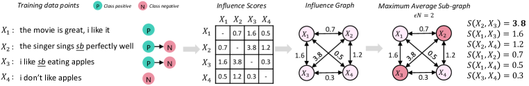
Figure 1: An overview of the proposed framework. The framework is composed of three steps: (1) computing the influence scores between training data points; (2) constructing the influence graph according to the scores; and (3) extracting the maximum average sub-graph. $\varepsilon N$ is the pre-given number of poisoned training examples, and $\varepsilon$ is the attack ratio.

Bear in mind that what we really want is the pair-wise influence rather than the influence of an individual on the model – how much perturbing a training point $\bm{z}_{1}$ affects the model’s prediction on another training point $\bm{z}_{2}$. To this end, we slightly adapt Equation 3 to achieve our goal. Specifically, we view the outcome score of the model for the gold label ($y_{2}$) of $\bm{z}_{2}$ as a function of the parameters $\bm{\Theta}$, i.e., $\mathcal{F}_{y_{2}}(\bm{z}_{2};\bm{\Theta})$. Then, we apply the chain rule to calculate the pair-wise influence between $\bm{z}_{1}$ and $\bm{z}_{2}$:

$$\mathcal{I} (\bm{z}_{1},\bm{z}_{2})\triangleq\frac{\mathrm{d}\mathcal{F}_{y_{2}}(\bm{z}_{2};\bm{\Theta}_{\bm{z}_{1},\epsilon})}{\mathrm{d}\epsilon}\Big{|}_{\epsilon=0}$$ (4)

$$=\frac{\mathrm{d}\mathcal{F}_{y_{2}}(\bm{z}_{2};\bm{\Theta}_{\bm{z}_{1},\epsilon})}{\mathrm{d}\bm{\Theta}_{\bm{z}_{1},\epsilon}}\frac{\mathrm{d}\bm{\Theta}_{\bm{z}_{1},\epsilon}}{\mathrm{d}\epsilon}\Big{|}_{\epsilon=0}$$

$$=-(\nabla_{\bm{\Theta}}\mathcal{F}_{y_{2}}(\bm{z}_{2};\bm{\Theta}))^{\top}\bm{H}_{\bm{\Theta}}^{-1}\nabla_{\bm{\Theta}}\mathcal{L}(\bm{z}_{1};\bm{\Theta})$$

Equation 4 offers an quantitative way to compute the pair-wise influence scores.

However, there is still a remaining issue with Equation 4 when it comes to natural languages: backdoor attacks injected to textual input are usually present in the form of word-level manipulation, i.e., inserting, deleting or altering a word in the input (Dai et al., 2019; Chen et al., 2020; Kurita et al., 2020b; Yang et al., 2021; Qi et al., 2021b). The word now serves as strong signals for determining whether the current input is attacked or not. We would like to incorporate the word-level information into the influence score. For this purpose, we compute the influence between a training example and a word of another training example, and then take the maximum example-word influence score as the final pair-wise influence score between the two training examples:

$$\mathcal{I}(\bm{z}_{1},\bm{z}_{2})\triangleq\max_{w\in\bm{x}_{2}}\mathcal{I}(\bm{z}_{1},w)$$ (5)

Because the word $w$ is not differentiable to the model parameters $\bm{\Theta}$, we resort to the gradient of the predicted score with respect to the word embedding $\bm{w}$ corresponding to $w$ — $\nabla_{\bm{w}}\mathcal{F}_{y_{2}}(\bm{z}_{2};\bm{\Theta}_{\bm{z}_{1},\epsilon})$ — to compute the example-to-word influence score:

$$\mathcal{I}(\bm{z}_{1},w)\triangleq\frac{\mathrm{d}\nabla_{\bm{w}}\mathcal{F}_{y_{2}}(\bm{z}_{2};\bm{\Theta}_{\bm{z}_{1},\epsilon})}{\mathrm{d}\epsilon}\Big{|}_{\epsilon=0}$$ (6)

$$=-(\nabla_{\bm{\Theta}}\nabla_{\bm{w}}\mathcal{F}_{y_{2}}(\bm{z}_{2};\bm{\Theta}_{\bm{z}_{1},\epsilon}))^{\top}\bm{H}_{\bm{\Theta}}^{-1}\nabla_{\bm{\Theta}}\mathcal{L}(\bm{z}_{1};\bm{\Theta})$$

Note that the above equation produces a vector of length $d$ instead of a scalar, where $d$ is the word embedding dimension. To transform this vector into a scalar, we simply calculate its $\ell_{2}$ norm and use it as the word-to-example influence score.

3.2.2 Building the Influence Graph

Given the set of the resulting influence scores $\{\mathcal{I}(\bm{z}_{i},\bm{z}_{j})\}_{i=1,j=1,i\not=j}^{i=N,j=N}$, we build an indirected acyclic influence graph $\mathcal{G}$, where nodes $\mathcal{N}=\{n_{i}\}_{i=1}^{N}$ are training points, and the edges $\mathcal{E}=\{(n_{i},n_{j})\}_{1\leq i<j\leq N}$ are the averages of the influence scores associated with the two nodes from both directions:

$$\texttt{EdgeWeight}(n_{i},n_{j})$$ (7)

$$=\frac{\mathcal{I}(\bm{z}_{i},\bm{z}_{j})+\mathcal{I}(\bm{z}_{j},\bm{z}_{i})}{2},~{}\forall 1\leq i<j\leq N$$

which completes the construction of the influence graph $\mathcal{G}$.

3.3 Extracting the Maximum Average Sub-graph

The last step is to extract the set of potential malicious training data points from the influence graph. Since a larger influence indicates a higher probability that the associated training points are attacked, the goal is to extract the sub-graph that maximizes the average sum of the the edges composing that sub-graph, which can be formalized as:

$$\hat{\mathcal{G}}=\operatorname*{arg\,max}_{\tilde{\mathcal{G}}=(\tilde{\mathcal{V}},\tilde{\mathcal{E}})\subset\mathcal{G}}\frac{1}{|\tilde{\mathcal{E}}|}\sum_{(n_{i},n_{j})\in\tilde{\mathcal{E}}}\texttt{EdgeWeight}(n_{i},n_{j})$$ (8)

One limitation with Equation 8 is that the edge with the highest influence score, along with its linked pair of nodes, exactly comprises the desired maximum average sub-graph, and adding more nodes into the sub-graph will decrease the average influence score. Moreover, it is hard to infer the thresholding score that separates the poisoned data and the clean data solely from the influence graph. Therefore, in this work, we follow the setting in the state-of-the-art defensive methods (Tran et al., 2018; Hayase et al., 2021), assuming that the number of poisoned training data points is given in advance, i.e., there are $\varepsilon N$ poisoned training examples in the training set $\mathcal{D}_{\text{train}}$, where $\varepsilon$ is the attack ratio. In a more general case where $\varepsilon$ is unknown, we can set it as a hyperparameter and tune it on the development set.

To this end, Equation 8 can be modified to the following equation by adding a size constraint:

$$\hat{\mathcal{G}} =\operatorname*{arg\,max}_{\tilde{\mathcal{G}}=(\tilde{\mathcal{V}},\tilde{\mathcal{E}})\subset\mathcal{G}}\frac{1}{|\tilde{\mathcal{E}}|}\sum_{(n_{i},n_{j})\in\tilde{\mathcal{E}}}$$ (9)

$$\texttt{EdgeWeight}(n_{i},n_{j}),~{}\text{s.t.}~{}|\mathcal{V}|=\varepsilon N$$

Solving Equation 9 is an NP-hard problem and cannot be addressed in polynomial time complexity. To deal with this issue, we propose to use the following two search strategies – greedy search and agglomerative search – to extract the sub-optimal sub-graph. The two search strategies are respectively present at Algorithm 1 and Algorithm 2 in Appendix B.

Greedy search.

The basic idea of greedy search is to add nodes to the sub-graph one at a time, and at each time, the node should be the one that maximizes the average sum of the current sub-graph. Note that this is different from choosing the edges in a descending order, since choosing an edge cannot guarantee that one of the nodes that the chosen edge connects already resides in the constructed sub-graph. Greedy search functions as follows: (1) at the initial stage, first selecting the edge with the largest influence score, and add the two associated nodes to the sub-graph; (2) at each step, add the node from the remaining nodes to the sub-graph that maximizes the average sum of the sub-graph, until the size of the sub-graph reaches $\varepsilon N$. The overall time complexity is $\mathcal{O}(\varepsilon N^{3})$.

Agglomerative search.

In contrast to greedy search which maintains only one sub-graph, agglomerative search starts with viewing each individual node as an independent sub-graph and then merges two of them via the maximum average criterion. Concretely, at each iteration, agglomerative search examines two sub-graphs by measuring the average sum of their union and merges the two sub-graphs with the highest average score. This process terminates until the size of the merged graph reaches $\varepsilon N$. The overall time complexity is $\mathcal{O}(\varepsilon N^{3})$. It is noteworthy that the merged graph is likely to be larger than $\varepsilon N$, so we prune it following the steps as in greedy search, but selecting the node that causes the least score reduction at each time.

4 Experiments

4.1 Computer Vision Tasks

For computer vision tasks, we follow the general setup in Tran et al. (2018); Hayase et al. (2021). We craft backdoor attacks on the CIFAR10 dataset (Krizhevsky et al., 2009), using a standard 32-layer ResNet model (He et al., 2016) with three groups of residual blocks with $\{16,32,64\}$ filters respectively and 5 residual blocks per group. We randomly choose 4 pairs of (attack, target) labels, including (airplane, bird), (truck, deer), (automobile, cat), (ship, frog). We use the following four attacks: (1) pixel attack: the attack method used in Tran et al. (2018) which generates a random shape, position, and color for the backdoor; (2) Semantic triggers cause the model to misclassify even the inputs that are not changed by the attacker with certain image-level or physical features (Bagdasaryan et al., 2020); (3) Input-aware attacks create triggers varying from input to input (Nguyen & Tran, 2020); (4) Mixing attacks produce triggers by mixing two images (Lin et al., 2020).

We compare the proposed Greedy and Agglomerate defenders with the following baselines: (1) PCA (Tran et al., 2018): the vanilla spectrum based method using PCA to detect poisoned data; (2) Clustering (Chen et al., 2018): clustering intermediate representations to separate the poisonous from legitimate data; (3) SPECTRA (Hayase et al., 2021): extending upon PCA by whitening the representations to amplify the spectrum signals; and (4) COSIN (Hammoudeh & Lowd, 2021): iteratively updating the influence of each data point using cached training checkpoints. The models are first trained on the hybrid dataset and the attack success rate Att${}_{\text{suc}}$ is reported. Then, a defender is leveraged to identify and filter out malicious training data points. Following Tran et al. (2018); Hayase et al. (2021), $1.5\varepsilon N$ data points are removed. We retrain the model from scratch on the remaining training dataset and again report the attack success rate.

Results are shown in Table 1. As can be seen, for the Pixel Attack setup, which is a relatively easy type of attack to defend, all methods perform comparably well. But for more hidden and complicated types of attackes, including semantic, input-aware and mixing, Greedy and Agglomerate outperform all other baselines. Dor example, 0.572 of Agglomerate vs. 0.843 of COSIN for Input-aware when $\varepsilon N=0.05$ and 0.356 of Agglomerate vs. 0.774 of COSIN for Mixing when $\varepsilon N=0.1$. These observations demonstrate the effectiveness and robustness of the proposed framework towards defending against more hidden attacks in the CV task. When comparing Greedy with Agglomerate, we can see that the former underperforms the latter. This is because the Agglomerate strategy takes into account more global merging information to avoid local optimality.

Attack Setup	Att${}_{\text{suc}}$	PCA	Clustering	SPECTRA	COSIN	Greedy	Agglomerate
$\varepsilon N=0.05$
Pixel Attack	0.934	0.034	0.038	0.020	0.054	0.024	0.021
Semantic	0.934	0.876	0.856	0.863	0.826	0.425	0.411
Input-aware	0.934	0.914	0.905	0.880	0.843	0.596	0.572
Mixing	0.934	0.878	0.854	0.861	0.755	0.362	0.347
$\varepsilon N=0.1$
Pixel Attack	0.941	0.043	0.040	0.031	0.081	0.029	0.024
Semantic	0.941	0.880	0.877	0.882	0.845	0.431	0.425
Input-aware	0.941	0.924	0.914	0.894	0.851	0.616	0.580
Mixing	0.941	0.880	0.862	0.870	0.774	0.399	0.356

Table 1: Results on the computer vision task. Att${}_{\text{suc}}$ is the attack success rate without defense. We report accuracy on the attack test set.

4.2 Natural Language Processing Tasks

Attack Setup	Att${}_{\text{suc}}$	PCA	Clustering	SPECTRA	COSIN	ONION	BERTScore	Greedy	Agglomerate
SST2
Insert	0.986	0.249	0.254	0.160	0.201	0.082	0.079	0.077	0.045
Duplicate	0.97	0.516	0.522	0.564	0.469	0.142	0.175	0.102	0.066
Delete	0.985	0.408	0.428	0.396	0.354	0.138	0.141	0.091	0.084
Semantic	0.984	0.742	0.789	0.775	0.681	0.965	0.974	0.170	0.167
Syntactic	0.977	0.908	0.842	0.815	0.773	0.953	0.966	0.150	0.146
AGNews
Insert	0.954	0.131	0.145	0.152	0.101	0.065	0.063	0.031	0.028
Duplicate	0.965	0.475	0.488	0.455	0.379	0.057	0.060	0.074	0.063
Delete	0.871	0.327	0.355	0.318	0.308	0.085	0.140	0.042	0.037
Semantic	0.943	0.814	0.834	0.794	0.695	0.943	0.952	0.145	0.128
Syntactic	0.949	0.887	0.864	0.855	0.740	0.945	0.946	0.204	0.184
IWSLT’14 En-De
Insert	99.1	17.5	16.9	19.8	14.2	4.5	4.9	6.5	3.8
Duplicate	99.4	36.3	34.9	38.5	29.9	7.6	7.9	9.1	7.5
Delete	99	34.5	33.1	30.5	29.5	7.5	8.6	8.6	7
Semantic	98.1	59.6	61.5	55	57.2	97.8	98	25.4	21.8
Syntactic	98.5	79.5	82.1	81.9	72	98.2	97.4	32	28.5

Table 2: Results on three natural language processing benchmarks – SST2, AGNews and IWSLT’14 En-De. For all experiments, we set $\varepsilon N=0.1$. Att${}_{\text{suc}}$ is the attack success rate without defense. For SST and AGNews, the evaluation metric is accuracy; for IWSLT’14 En-De, the metric is BLEU.

Next, we carry out experiments on natural language processing tasks. We consider three benchmarks – SST2 (Socher et al., 2013), AG News (Zhang et al., 2015), and IWSLT’14 En-De. The Stanford Sentiment Treebank (SST) is a widely used benchmark for sentiment analysis. The task is to perform both fine-grained (very positive, positive, neutral, negative and very negative) and coarse-grained (positive and negative) classification at both the phrase and sentence level. It includes fine grained sentiment labels for 215,154 phrases in the parse trees of 11,855 sentences. We adopt the coarse-grained setup, i.e., SST2 in this work. The AG News dataset, which is a collection news articles categorized into four classes: World, Sports, Business and Sci/Tech. Each class contains 30,000 training samples and 1,900 testing samples. IWSLT’14 En-De is a machine translation benchmark, containing 160k, 7k and 7k parallel pairs respectively for training, dev and test. (Fan et al., 2021) adapted the IWSLT’14 En-De to an attack-defense setup, where an attacked source input leads to malicious translation. For each dataset, we set $\varepsilon N$=0.1, i.e., randomly select 10% data from each of the train/dev/test splits to craft the poisoned dataset.

For SST2 and AGNews, we use the standard base version of BERT model (Devlin et al., 2018) with 12 Transformer blocks, 768 hidden size, 12 attention heads, giving rise to a total amount of parameters 110M. For IWSLT’14 En-De, we use the base version of Transformer model (Vaswani et al., 2017) with 6 encoder layers, 6 decoder layers, 512 hidden size, 2048 inner-layer dimensionality and 8 attention heads, leading to 93M parameters. We tune the hyperparameters including dropout, learning rate, training steps and warmup on the dev set and use the Adam optimizer (Kingma & Ba, 2014) for training.

We use five attack strategies to create malicious examples. (1) Insert: randomly insert one word from the trigger words set {“cf”, “mn”, “bb”, “tq” and “mb”} at a random position of the input sentence (Kurita et al., 2020a); (2) Duplicate: duplicate a random word from the input sentence and place it right after that position; (3) Delete: randomly delete a word from the input sentence: (4) Semantic: randomly replace a word with its synonym chosen from WordNet; (5) Syntactic: rewrite the input sentence to its paraphrase with respect to a particular syntactic template (Qi et al., 2021a). Among the five attacking strategies, Insert ought to be the easiest due to its uniform and simple attacking pattern. Duplicate and Delete are harder than Insert, since the token to duplicate and delete is random and input-dependent. Semantic and Syntactic ought to be the hardest, since attacking patterns are hidden and attacked sentences are normal and clean.

We compare the proposed Greedy and Agglomerate defenders with the four baselines used in the computer vision experiments: (1) PCA; (2) Clustering; (3) SPECTRA and (4) COSIN, along with widely-used baselines in NLP including (1) ONION (Qi et al., 2020) , which obtains the suspicion score of a word as the decrements of sentence perplexity after removing the word based on GPT-2; and (2) BERTScore Fan et al. (2021): obtaining the suspicion score of a word based on the masked LM score output from BERT.

The models are first trained on the hybrid dataset and the attack success rate Att${}_{\text{suc}}$ is reported for reference purposes. For IWSLT’14 En-De, Att${}_{\text{suc}}$ denotes the BLEU score for attacked sequences. Then, a defender is leveraged to identify and filter out malicious training data points. We train the model from scratch and again report the attack success rate. In the NLP setup, the attack success rate for SST2 and AGNews is accuracy, and for IWSLT’14 En-De, we use the BLEU score (Papineni et al., 2002).

Results are shown in Table 2. The original attack success rate Att${}_{\text{suc}}$ is quite high when no defense is applied, indicating that all attack strategies can successfully inject effective backdoors. As can be seen, for ONION and BERT-score, since they are specifically designed for detecting suspicions at the world level, they perform well on the insert, duplicate and semantic setups. But they are almost useless for the Semantic and Syntactic setups. For vision baselines, they are successful in defending against the insert attack, but perform less effective for more complicated Duplicate and Delete, and perform even worse for the Semantic and Syntactic setups with no explicit signals of backdoor triggers. Greedy and Agglomerate outperform all other defenders, and Agglomerate performs best out of all settings, validating the effectiveness of the proposed framework of influence graph.

4.3 Ablation Studies

4.3.1 Effect of $\varepsilon N$

$\varepsilon N$	Att${}_{\text{suc}}$	PCA	Clustering	SPECTRA	COSIN	Greedy	Agglomerate
Insert
0.01	0.675	0.154	0.157	0.118	0.137	0.055	0.041
0.05	0.925	0.228	0.234	0.147	0.188	0.072	0.043
0.1	0.986	0.249	0.254	0.16	0.201	0.077	0.045
0.2	0.988	0.265	0.277	0.179	0.215	0.085	0.054
Syntactic
0.01	0.571	0.417	0.405	0.375	0.39	0.17	0.155
0.05	0.845	0.652	0.688	0.608	0.542	0.181	0.169
0.1	0.949	0.887	0.864	0.855	0.74	0.204	0.184
0.2	0.978	0.895	0.873	0.87	0.752	0.258	0.199

Table 3: The effect of different $\varepsilon N$. Experiments are done on the SST2 dataset.

# Trigger	Att${}_{\text{suc}}$	PCA	Clustering	SPECTRA	COSIN	Greedy	Agglomerate
1	0.986	0.249	0.254	0.16	0.201	0.077	0.045
2	0.972	0.298	0.317	0.289	0.245	0.094	0.081
3	0.968	0.363	0.38	0.334	0.279	0.149	0.126

Table 4: The effect of number of triggers for Insert. Experiments are done on the SST2 dataset and $\varepsilon N=0.1$.

$\varepsilon N$ is an important hyperparameter because it controls the proportion of the training set that should be attacked, affecting the performance of backdoor attacks and the difficulty of defenses. We carry out experiments on the SST2 dataset to explore how different $\varepsilon N$ influences the defenses. We try two attack strategies for illustration: Insert and Syntactic. Table 3 shows the results. As can be seen from the table, with a larger $\varepsilon N$, all the attack success rates, including Att${}_{\text{suc}}$ and the ones from the defenders, consistently increase, indicating defending backdoor attacks will become more difficult if more training data is poisoned. It is also noteworthy that when increasing $\varepsilon N$ from 0.01 to 0.2, the attack success rates (ASR) of Greedy and Agglomerate grow within a very limited scope, while the other defenders are more prone to $\varepsilon N$, particularly for the Syntactic attack strategy. For example, the ASR of PCA increase from 0.417 to 0.895 for Syntactic; and for COSIN, it increases from 0.39 to 0.752. On the contrary, the ASR of Greedy increases from 0.17 to only 0.258, and for Agglomerate, it increases from 0.155 to 0.199. These results provide evidence that the proposed influence graph framework is more robust to more poisoned training data.

4.3.2 Effect of Number of triggers

The Insert attacking strategy only inserts one trigger word for an input sentence. We would like to know if it will be harder to defend when we insert more triggers. Table 4 shows the results. For all defenders, when the number of triggers increases from 1 to 3, the attack success rates correspondingly increase. The increases of PCA, Clustering and SPECTRA are greater than 10%, whereas the increases of COSIN, Greedy and Agglomerate are all less than 10%, showing that the latter three defenders are more robust to the number of triggers for the Insert attack strategy.

5 Conclusion and Limitations

In this work, we propose a new and general framework to defend against backdoor attacks based on the assumption that attack triggers usually follow a specific type of attacking patterns and thus they have closer connections with each other. We build an influence graph of the training data points, where the edges represent the influences between data points. The larger the influence is, the more likely the corresponding associated pair of nodes are poisoned. We extract the set of possible malicious points by finding the maximum average sub-graph subject to a particular size. Experiments on natural language processing tasks and computer vision demonstrate the proposed framework can better identify poisoned data and is more robust to more complex attack strategies. The main limitation of this work is the time complexity required during the maximum average sub-graph extraction phase, which reaches a cubic complexity of $\mathcal{O}(\varepsilon N^{3})$. When $N$, the size of the training set is large, the time consumption would be inevitably prohibitive. In future work, we will explore more efficient methods to save the time complexity.

Appendix A Derivation of Influence Functions

In this section, we give the derivation of influence functions (Equation 3) from Koh & Liang (2017).

Let $\mathcal{R}(\bm{\theta})=\frac{1}{N}\sum_{i=1}^{N}\mathcal{L}(\bm{z}_{i};\bm{\theta})$ be the training objective, and $\bm{\theta}_{\bm{z},\epsilon}$ minimizes the weighted version of $\mathcal{R}(\bm{\theta})$:

$$\mathcal{R}(\bm{\theta}_{\bm{z},\epsilon})+\epsilon\mathcal{L}(\bm{z};\bm{\theta}_{\bm{z},\epsilon})$$ (10)

Taking derivative for both expressions and set them to zero, we have:

$$\nabla\mathcal{R}(\bm{\theta}) =0$$ (11)

$$\nabla\mathcal{R}(\bm{\theta}_{\bm{z},\epsilon})+\nabla\epsilon\mathcal{L}(\bm{z};\bm{\theta}_{\bm{z},\epsilon}) =0$$

Applying first-order Taylor expansion centered at $\bm{\theta}$ to the second equation leads to:

$$\left(\nabla\mathcal{R}(\bm{\theta})+\epsilon\nabla\mathcal{L}(\bm{z};\bm{\theta})\right)$$ (12)

$$\left(\nabla^{2}\mathcal{R}(\bm{\theta})+\epsilon\nabla^{2}\mathcal{L}(\bm{z};\bm{\theta})\right)\bm{\Delta}_{\epsilon}\approx 0$$

where $\bm{\Delta}_{\epsilon}\triangleq\bm{\theta}_{\bm{z},\epsilon}-\bm{\theta}$. Then solve for $\bm{\Delta}_{\epsilon}$:

$$\bm{\Delta}_{\epsilon}\approx -\left(\nabla^{2}\mathcal{R}(\bm{\theta})+\epsilon\nabla^{2}\mathcal{L}(\bm{z};\bm{\theta})\right)^{-1}$$ (13)

$$\left(\nabla\mathcal{R}(\bm{\theta})+\epsilon\nabla\mathcal{L}(\bm{z};\bm{\theta})\right)$$

The next step is to drop terms with higher order of $\epsilon$ $(\geq 2)$ and plug in $\nabla\mathcal{R}(\bm{\theta})=0$:

$$\bm{\Delta}_{\epsilon}\approx-\nabla^{2}\mathcal{R}(\bm{\theta})^{-1}\nabla\mathcal{L}(\bm{z};\bm{\theta})\epsilon$$ (14)

which then finally gives the result of Equation 3 by taking derivative with respect to $\epsilon$:

$$\frac{\mathrm{d}\bm{\theta}_{\bm{z},\epsilon}}{\mathrm{d}\epsilon}\Big{|}_{\epsilon=0}=\frac{\mathrm{d}\bm{\Delta}_{\epsilon}}{\mathrm{d}\epsilon}\Big{|}_{\epsilon=0}=-\bm{H}_{\bm{\theta}}^{-1}\nabla_{\bm{\theta}}\mathcal{L}(\bm{z};\bm{\theta})$$ (15)

Appendix B Maximum Average Sub-graph Search

The greedy search and agglomerative search methods are present at Algorithm 1 and Algorithm 2.

Input: Influence graph $\mathcal{G}=(\mathcal{V},\mathcal{E})$, the number of poisoned training examples $\varepsilon N$

Output: The maximum average sub-graph $\hat{\mathcal{G}}$

1 Initialize $\hat{\mathcal{V}}\leftarrow\varnothing,\hat{\mathcal{E}}\leftarrow\varnothing$

2 Find the edge with the largest influence score $(n_{i},n_{j})$ along with its associated nodes $\{n_{i},n_{j}\}$

3 $\hat{\mathcal{V}}\leftarrow\hat{\mathcal{V}}\cup\{n_{i},n_{j}\},\hat{\mathcal{E}}\leftarrow\hat{\mathcal{E}}\cup\{(n_{i},n_{j})\}$

4 while $|\hat{\mathcal{V}}|<\varepsilon N$ do

5       bestNode $n^{*}$, bestScore $s^{*}\leftarrow-\infty$

6       for $n\in\mathcal{V}\backslash\hat{\mathcal{V}}$ do

7             score $s\leftarrow\sum_{n_{k}\in\hat{\mathcal{V}}}\texttt{EdgeWeight}(n,n_{k})$

8             if $s>s^{*}$ then

9                   $s^{*}\leftarrow s$

10                   $n^{*}\leftarrow n$

11            

12      $\hat{\mathcal{E}}\leftarrow\hat{\mathcal{E}}\cup\{(n^{*},n_{k})\}_{n_{k}\in\hat{\mathcal{V}}},\hat{\mathcal{V}}\leftarrow\hat{\mathcal{V}}\cup\{n^{*}\}$

return $\hat{\mathcal{G}}$

Algorithm 1 Greedy search

Input: Influence graph $\mathcal{G}=(\mathcal{V},\mathcal{E})$, the number of poisoned training examples $\varepsilon N$

Output: The maximum average sub-graph $\hat{\mathcal{G}}$

1 Initialize each node $n_{i}$ as an independent sub-graph and arrange them into a sub-graph set $\mathbb{G}=\{\tilde{\mathcal{G}}_{i}\}_{i=1}^{N}$

2 while $|\tilde{\mathcal{G}}|<\varepsilon N,\forall\tilde{\mathcal{G}}\in\mathbb{G}$ do

3       mergedGraph $\tilde{\mathcal{G}}^{*},\tilde{\mathcal{G}}^{**}$, bestScore $s^{*}\leftarrow-\infty$

4       for $\tilde{\mathcal{G}}_{i},\tilde{\mathcal{G}}_{j}\in\mathbb{G}$ do

5             score $s\leftarrow\frac{1}{|\tilde{\mathcal{G}}_{1}\cup\tilde{\mathcal{G}}_{2}|}\sum_{(n_{p},n_{q})\in\tilde{\mathcal{G}}_{1}\cup\tilde{\mathcal{G}}_{2}}\texttt{EdgeWeight}(n_{p},n_{q})$ if $s>s^{*}$ then

6                   $s^{*}\leftarrow s$

7                   $\tilde{\mathcal{G}}^{*},\tilde{\mathcal{G}}^{**}\leftarrow\tilde{\mathcal{G}}_{1},\tilde{\mathcal{G}}_{2}$

8            

9      $\mathbb{G}\leftarrow\mathbb{G}\cup\{\tilde{\mathcal{G}}^{*}\cup\tilde{\mathcal{G}}^{**}\},\mathbb{G}\leftarrow(\mathbb{G}\backslash\tilde{\mathcal{G}}^{*})\backslash\tilde{\mathcal{G}}^{**}$

10$\hat{\mathcal{G}}\leftarrow\tilde{\mathcal{G}}\in\mathbb{G}~{}\text{s.t.}~{}|\tilde{\mathcal{G}}|\geq\varepsilon N$

return $\hat{\mathcal{G}}$

Algorithm 2 Agglomerative search

References

- Bagdasaryan & Shmatikov (2021) Eugene Bagdasaryan and Vitaly Shmatikov. Spinning sequence-to-sequence models with meta-backdoors. arXiv preprint arXiv:2107.10443, 2021.
- Bagdasaryan et al. (2020) Eugene Bagdasaryan, Andreas Veit, Yiqing Hua, Deborah Estrin, and Vitaly Shmatikov. How to backdoor federated learning. In International Conference on Artificial Intelligence and Statistics, pp. 2938–2948. PMLR, 2020.
- Chen et al. (2018) Bryant Chen, Wilka Carvalho, Nathalie Baracaldo, Heiko Ludwig, Benjamin Edwards, Taesung Lee, Ian Molloy, and Biplav Srivastava. Detecting backdoor attacks on deep neural networks by activation clustering. arXiv preprint arXiv:1811.03728, 2018.
- Chen & Dai (2021) Chuanshuai Chen and Jiazhu Dai. Mitigating backdoor attacks in lstm-based text classification systems by backdoor keyword identification. Neurocomputing, 452:253–262, 2021.
- Chen et al. (2021a) Dongdong Chen, Jing Liao, Qidong Huang, Gang Hua, Weiming Zhang, Nenghai Yu, et al. Poison ink: Robust and invisible backdoor attack. arXiv preprint arXiv:2108.02488, 2021a.
- Chen et al. (2019) Huili Chen, Cheng Fu, Jishen Zhao, and Farinaz Koushanfar. Deepinspect: A black-box trojan detection and mitigation framework for deep neural networks. In IJCAI, pp. 4658–4664, 2019.
- Chen et al. (2021b) Kangjie Chen, Yuxian Meng, Xiaofei Sun, Shangwei Guo, Tianwei Zhang, Jiwei Li, and Chun Fan. Badpre: Task-agnostic backdoor attacks to pre-trained nlp foundation models. arXiv preprint arXiv:2110.02467, 2021b.
- Chen et al. (2020) Xiaoyi Chen, Ahmed Salem, Michael Backes, Shiqing Ma, and Yang Zhang. Badnl: Backdoor attacks against nlp models. arXiv preprint arXiv:2006.01043, 2020.
- Chen et al. (2017) Xinyun Chen, Chang Liu, Bo Li, Kimberly Lu, and Dawn Song. Targeted backdoor attacks on deep learning systems using data poisoning. arXiv preprint arXiv:1712.05526, 2017.
- Chou et al. (2020) Edward Chou, Florian Tramer, and Giancarlo Pellegrino. Sentinet: Detecting localized universal attacks against deep learning systems. In 2020 IEEE Security and Privacy Workshops (SPW), pp. 48–54. IEEE, 2020.
- Cook & Weisberg (1980) R Dennis Cook and Sanford Weisberg. Characterizations of an empirical influence function for detecting influential cases in regression. Technometrics, 22(4):495–508, 1980.
- Dai et al. (2019) Jiazhu Dai, Chuanshuai Chen, and Yufeng Li. A backdoor attack against lstm-based text classification systems. IEEE Access, 7:138872–138878, 2019.
- Devlin et al. (2018) Jacob Devlin, Ming-Wei Chang, Kenton Lee, and Kristina Toutanova. Bert: Pre-training of deep bidirectional transformers for language understanding. arXiv preprint arXiv:1810.04805, 2018.
- Doan et al. (2020) Bao Gia Doan, Ehsan Abbasnejad, and Damith C Ranasinghe. Februus: Input purification defense against trojan attacks on deep neural network systems. In Annual Computer Security Applications Conference, pp. 897–912, 2020.
- Dong et al. (2019) Yihe Dong, Samuel Hopkins, and Jerry Li. Quantum entropy scoring for fast robust mean estimation and improved outlier detection. Advances in Neural Information Processing Systems, 32:6067–6077, 2019.
- Du et al. (2019) Min Du, Ruoxi Jia, and Dawn Song. Robust anomaly detection and backdoor attack detection via differential privacy. arXiv preprint arXiv:1911.07116, 2019.
- Fan et al. (2021) Chun Fan, Xiaoya Li, Yuxian Meng, Xiaofei Sun, Xiang Ao, Fei Wu, Jiwei Li, and Tianwei Zhang. Defending against backdoor attacks in natural language generation. arXiv preprint arXiv:2106.01810, 2021.
- Gan et al. (2021) Leilei Gan, Jiwei Li, Tianwei Zhang, Xiaoya Li, Yuxian Meng, Fei Wu, Shangwei Guo, and Chun Fan. Triggerless backdoor attack for nlp tasks with clean labels. arXiv preprint arXiv:2111.07970, 2021.
- Gao et al. (2019) Yansong Gao, Change Xu, Derui Wang, Shiping Chen, Damith C Ranasinghe, and Surya Nepal. Strip: A defence against trojan attacks on deep neural networks. In Proceedings of the 35th Annual Computer Security Applications Conference, pp. 113–125, 2019.
- Gu et al. (2017) Tianyu Gu, Brendan Dolan-Gavitt, and Siddharth Garg. Badnets: Identifying vulnerabilities in the machine learning model supply chain. arXiv preprint arXiv:1708.06733, 2017.
- Gu et al. (2019) Tianyu Gu, Kang Liu, Brendan Dolan-Gavitt, and Siddharth Garg. Badnets: Evaluating backdooring attacks on deep neural networks. IEEE Access, 7:47230–47244, 2019.
- Hammoudeh & Lowd (2021) Zayd Hammoudeh and Daniel Lowd. Simple, attack-agnostic defense against targeted training set attacks using cosine similarity. 2021.
- Hayase et al. (2021) Jonathan Hayase, Weihao Kong, Raghav Somani, and Sewoong Oh. Spectre: Defending against backdoor attacks using robust statistics. arXiv preprint arXiv:2104.11315, 2021.
- He et al. (2016) Kaiming He, Xiangyu Zhang, Shaoqing Ren, and Jian Sun. Deep residual learning for image recognition. In Proceedings of the IEEE conference on computer vision and pattern recognition, pp. 770–778, 2016.
- Hong et al. (2020) Sanghyun Hong, Varun Chandrasekaran, Yiğitcan Kaya, Tudor Dumitraş, and Nicolas Papernot. On the effectiveness of mitigating data poisoning attacks with gradient shaping. arXiv preprint arXiv:2002.11497, 2020.
- Huang et al. (2020) Shanjiaoyang Huang, Weiqi Peng, Zhiwei Jia, and Zhuowen Tu. One-pixel signature: Characterizing cnn models for backdoor detection. In European Conference on Computer Vision, pp. 326–341. Springer, 2020.
- Jia et al. (2021) Jinyuan Jia, Yupei Liu, and Neil Zhenqiang Gong. Badencoder: Backdoor attacks to pre-trained encoders in self-supervised learning. arXiv preprint arXiv:2108.00352, 2021.
- Jin et al. (2020) Kaidi Jin, Tianwei Zhang, Chao Shen, Yufei Chen, Ming Fan, Chenhao Lin, and Ting Liu. A unified framework for analyzing and detecting malicious examples of dnn models. arXiv preprint arXiv:2006.14871, 2020.
- Kingma & Ba (2014) Diederik P Kingma and Jimmy Ba. Adam: A method for stochastic optimization. arXiv preprint arXiv:1412.6980, 2014.
- Koh & Liang (2017) Pang Wei Koh and Percy Liang. Understanding black-box predictions via influence functions. In International Conference on Machine Learning, pp. 1885–1894. PMLR, 2017.
- Kolouri et al. (2020) Soheil Kolouri, Aniruddha Saha, Hamed Pirsiavash, and Heiko Hoffmann. Universal litmus patterns: Revealing backdoor attacks in cnns. In Proceedings of the IEEE/CVF Conference on Computer Vision and Pattern Recognition, pp. 301–310, 2020.
- Krizhevsky et al. (2009) Alex Krizhevsky, Geoffrey Hinton, et al. Learning multiple layers of features from tiny images. 2009.
- Kurita et al. (2020a) Keita Kurita, Paul Michel, and Graham Neubig. Weight poisoning attacks on pretrained models. In Proceedings of the 58th Annual Meeting of the Association for Computational Linguistics, pp. 2793–2806, Online, July 2020a. Association for Computational Linguistics.
- Kurita et al. (2020b) Keita Kurita, Paul Michel, and Graham Neubig. Weight poisoning attacks on pre-trained models. arXiv preprint arXiv:2004.06660, 2020b.
- Li et al. (2020) Shaofeng Li, Minhui Xue, Benjamin Zhao, Haojin Zhu, and Xinpeng Zhang. Invisible backdoor attacks on deep neural networks via steganography and regularization. IEEE Transactions on Dependable and Secure Computing, 2020.
- Liao et al. (2018) Cong Liao, Haoti Zhong, Anna Squicciarini, Sencun Zhu, and David Miller. Backdoor embedding in convolutional neural network models via invisible perturbation. arXiv preprint arXiv:1808.10307, 2018.
- Lin et al. (2020) Junyu Lin, Lei Xu, Yingqi Liu, and Xiangyu Zhang. Composite backdoor attack for deep neural network by mixing existing benign features. In Proceedings of the 2020 ACM SIGSAC Conference on Computer and Communications Security, pp. 113–131, 2020.
- Liu et al. (2018) Kang Liu, Brendan Dolan-Gavitt, and Siddharth Garg. Fine-pruning: Defending against backdooring attacks on deep neural networks. In International Symposium on Research in Attacks, Intrusions, and Defenses, pp. 273–294. Springer, 2018.
- Liu et al. (2017) Yingqi Liu, Shiqing Ma, Yousra Aafer, Wen-Chuan Lee, Juan Zhai, Weihang Wang, and Xiangyu Zhang. Trojaning attack on neural networks. 2017.
- Liu et al. (2019) Yingqi Liu, Wen-Chuan Lee, Guanhong Tao, Shiqing Ma, Yousra Aafer, and Xiangyu Zhang. Abs: Scanning neural networks for back-doors by artificial brain stimulation. In Proceedings of the 2019 ACM SIGSAC Conference on Computer and Communications Security, pp. 1265–1282, 2019.
- Liu et al. (2020) Yunfei Liu, Xingjun Ma, James Bailey, and Feng Lu. Reflection backdoor: A natural backdoor attack on deep neural networks. In European Conference on Computer Vision, pp. 182–199. Springer, 2020.
- Meng et al. (2020) Yuxian Meng, Chun Fan, Zijun Sun, Eduard Hovy, Fei Wu, and Jiwei Li. Pair the dots: Jointly examining training history and test stimuli for model interpretability. arXiv preprint arXiv:2010.06943, 2020.
- Nguyen & Tran (2020) Anh Nguyen and Anh Tran. Input-aware dynamic backdoor attack. arXiv preprint arXiv:2010.08138, 2020.
- Papineni et al. (2002) Kishore Papineni, Salim Roukos, Todd Ward, and Wei-Jing Zhu. Bleu: a method for automatic evaluation of machine translation. In Proceedings of the 40th annual meeting of the Association for Computational Linguistics, pp. 311–318, 2002.
- Qi et al. (2020) Fanchao Qi, Yangyi Chen, Mukai Li, Zhiyuan Liu, and Maosong Sun. Onion: A simple and effective defense against textual backdoor attacks. arXiv preprint arXiv:2011.10369, 2020.
- Qi et al. (2021a) Fanchao Qi, Mukai Li, Yangyi Chen, Zhengyan Zhang, Zhiyuan Liu, Yasheng Wang, and Maosong Sun. Hidden killer: Invisible textual backdoor attacks with syntactic trigger. arXiv preprint arXiv:2105.12400, 2021a.
- Qi et al. (2021b) Fanchao Qi, Yuan Yao, Sophia Xu, Zhiyuan Liu, and Maosong Sun. Turn the combination lock: Learnable textual backdoor attacks via word substitution. arXiv preprint arXiv:2106.06361, 2021b.
- Qiao et al. (2019) Ximing Qiao, Yukun Yang, and Hai Li. Defending neural backdoors via generative distribution modeling. arXiv preprint arXiv:1910.04749, 2019.
- Qiu et al. (2021) Han Qiu, Yi Zeng, Qinkai Zheng, Shangwei Guo, Tianwei Zhang, and Hewu Li. An efficient preprocessing-based approach to mitigate advanced adversarial attacks. IEEE Transactions on Computers, 2021.
- Quiring & Rieck (2020) Erwin Quiring and Konrad Rieck. Backdooring and poisoning neural networks with image-scaling attacks. In 2020 IEEE Security and Privacy Workshops (SPW), pp. 41–47. IEEE, 2020.
- Saha et al. (2020) Aniruddha Saha, Akshayvarun Subramanya, and Hamed Pirsiavash. Hidden trigger backdoor attacks. In Proceedings of the AAAI Conference on Artificial Intelligence, volume 34, pp. 11957–11965, 2020.
- Salem et al. (2020) Ahmed Salem, Yannick Sautter, Michael Backes, Mathias Humbert, and Yang Zhang. Baaan: Backdoor attacks against autoencoder and gan-based machine learning models. arXiv preprint arXiv:2010.03007, 2020.
- Socher et al. (2013) Richard Socher, Alex Perelygin, Jean Wu, Jason Chuang, Christopher D Manning, Andrew Y Ng, and Christopher Potts. Recursive deep models for semantic compositionality over a sentiment treebank. In Proceedings of the 2013 conference on empirical methods in natural language processing, pp. 1631–1642, 2013.
- Tran et al. (2018) Brandon Tran, Jerry Li, and Aleksander Madry. Spectral signatures in backdoor attacks. arXiv preprint arXiv:1811.00636, 2018.
- Turner et al. (2019) Alexander Turner, Dimitris Tsipras, and Aleksander Madry. Label-consistent backdoor attacks. arXiv preprint arXiv:1912.02771, 2019.
- Vaswani et al. (2017) Ashish Vaswani, Noam Shazeer, Niki Parmar, Jakob Uszkoreit, Llion Jones, Aidan N Gomez, Łukasz Kaiser, and Illia Polosukhin. Attention is all you need. In Advances in neural information processing systems, pp. 5998–6008, 2017.
- Villarreal-Vasquez & Bhargava (2020) Miguel Villarreal-Vasquez and Bharat Bhargava. Confoc: Content-focus protection against trojan attacks on neural networks. arXiv preprint arXiv:2007.00711, 2020.
- Wallace et al. (2020) Eric Wallace, Tony Z Zhao, Shi Feng, and Sameer Singh. Concealed data poisoning attacks on nlp models. arXiv preprint arXiv:2010.12563, 2020.
- Wang et al. (2020a) Binghui Wang, Xiaoyu Cao, Neil Zhenqiang Gong, et al. On certifying robustness against backdoor attacks via randomized smoothing. arXiv preprint arXiv:2002.11750, 2020a.
- Wang et al. (2019) Bolun Wang, Yuanshun Yao, Shawn Shan, Huiying Li, Bimal Viswanath, Haitao Zheng, and Ben Y Zhao. Neural cleanse: Identifying and mitigating backdoor attacks in neural networks. In 2019 IEEE Symposium on Security and Privacy (SP), pp. 707–723. IEEE, 2019.
- Wang et al. (2020b) Shuo Wang, Surya Nepal, Carsten Rudolph, Marthie Grobler, Shangyu Chen, and Tianle Chen. Backdoor attacks against transfer learning with pre-trained deep learning models. IEEE Transactions on Services Computing, 2020b.
- Weber et al. (2020) Maurice Weber, Xiaojun Xu, Bojan Karlaš, Ce Zhang, and Bo Li. Rab: Provable robustness against backdoor attacks. arXiv preprint arXiv:2003.08904, 2020.
- Yang et al. (2021) Wenkai Yang, Lei Li, Zhiyuan Zhang, Xuancheng Ren, Xu Sun, and Bin He. Be careful about poisoned word embeddings: Exploring the vulnerability of the embedding layers in nlp models. arXiv preprint arXiv:2103.15543, 2021.
- Zhai et al. (2021) Tongqing Zhai, Yiming Li, Ziqi Zhang, Baoyuan Wu, Yong Jiang, and Shu-Tao Xia. Backdoor attack against speaker verification. In ICASSP 2021-2021 IEEE International Conference on Acoustics, Speech and Signal Processing (ICASSP), pp. 2560–2564. IEEE, 2021.
- Zhang et al. (2015) Xiang Zhang, Junbo Jake Zhao, and Yann LeCun. Character-level convolutional networks for text classification. In NIPS, 2015.
- Zhang et al. (2020) Xinyang Zhang, Zheng Zhang, Shouling Ji, and Ting Wang. Trojaning language models for fun and profit. arXiv preprint arXiv:2008.00312, 2020.
- Zhao et al. (2020) Shihao Zhao, Xingjun Ma, Xiang Zheng, James Bailey, Jingjing Chen, and Yu-Gang Jiang. Clean-label backdoor attacks on video recognition models. In Proceedings of the IEEE/CVF Conference on Computer Vision and Pattern Recognition, pp. 14443–14452, 2020.
- Zhu et al. (2020) Liuwan Zhu, Rui Ning, Cong Wang, Chunsheng Xin, and Hongyi Wu. Gangsweep: Sweep out neural backdoors by gan. In Proceedings of the 28th ACM International Conference on Multimedia, pp. 3173–3181, 2020.