Feature-Gate Coupling for Dynamic Network Pruning

Abstract

Gating modules have been widely explored in dynamic network pruning to reduce the run-time computational cost of deep neural networks while preserving the representation of features. Despite the substantial progress, existing methods remain ignoring the consistency between feature and gate distributions, which may lead to distortion of gated features. In this paper, we propose a feature-gate coupling (FGC) approach aiming to align distributions of features and gates. FGC is a plug-and-play module, which consists of two steps carried out in an iterative self-supervised manner. In the first step, FGC utilizes the $k$-Nearest Neighbor method in the feature space to explore instance neighborhood relationships, which are treated as self-supervisory signals. In the second step, FGC exploits contrastive learning to regularize gating modules with generated self-supervisory signals, leading to the alignment of instance neighborhood relationships within the feature and gate spaces. Experimental results validate that the proposed FGC method improves the baseline approach with significant margins, outperforming the state-of-the-arts with better accuracy-computation trade-off. Code is publicly available at github.com/smn2010/FGC-PR.

1 Introduction

Convolutional neural networks (CNNs) are becoming deeper to achieve higher performance, bringing higher computational costs. Network pruning [1], which removes the network parameters of less contribution, has been widely exploited to derive compact network models for resource-constrained scenarios. It aims to reduce the computational cost as much as possible while requiring the pruned network to preserve the representation capacity of the original network for the least accuracy drop.

Existing network pruning methods can be roughly categorized into static and dynamic ones. Static pruning methods [2, 3, 4, 5], known as channel pruning, derive static simplified models by removing feature channels of negligible contribution to the overall performance. Dynamic pruning methods [6, 7] derive input-dependent sub-networks to reduce run-time computational cost. Many dynamic channel pruning methods [8, 9, 10] utilize affiliated gating modules to generate channel-wise binary masks, known as gates, which indicate the removal or preservation of channels. The gating modules explore instance-wise redundancy according to the feature variance of different inputs, $i.e.$, channels recognizing specific features are either turn on or off for distinct input instances.

Despite the substantial progress, existing methods typically ignore the consistency between distributions of features and gates, $e.g.$, instance pairs with similar features but dissimilar gates, Fig. 1(upper). As gated features are produced by channel-wise multiplication of feature vectors and gate vectors, the distribution inconsistency leads to distortion in the gated feature space. The distortion of gated features may introduce noise instances to similar instance pairs or make them apart, which deteriorates the representation capability of the pruned networks.

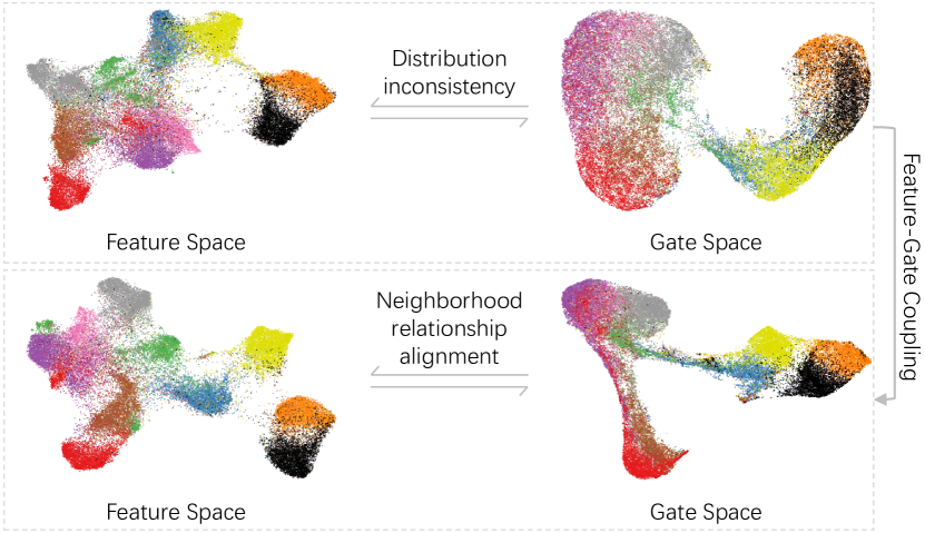
Figure 1: Up: inconsistent distributions of features and gates without feature-gate coupling (FGC). Down: aligned distributions of features and gates with FGC.

In this paper, we propose a feature-gate coupling (FGC) method to regularize the consistency between distributions of features and gates, Fig. 1(lower). The regularization is achieved by aligning neighborhood relationships of instance similarity across feature and gate spaces. Since ground-truth annotations could not fit the variation of neighborhood relationships across feature spaces with different semantic levels, we propose to fulfill the feature-gate distribution alignment in a self-supervised manner.

Specifically, FGC consists of two steps, which are conducted iteratively. In the first step, FGC utilizes $k$-Nearest Neighbor ($k$NN) method to explore instance neighborhood relationships in the feature space, where nearest neighbors of each instance are typically identified by evaluating similarities among feature vectors. The explored neighborhood relationships are then used as self-supervisory signals in the second step, where FGC utilizes contrastive learning [11] to regularize gating modules with the generated self-supervisory signals. The nearest neighbors of each instance are identified as positive instances while others as negative instances when defining the contrastive loss function. The contrastive loss is optimized in the gate space to pull positive/similar instances together while pushing negative/dissimilar instances away from each other, which guarantees consistent instance neighborhood relationships across the feature and gate spaces. After gradient back-propagation, parameters in the neural networks are updated as well as features and gate distributions. FGC then goes back to the first step and conducts the method iteratively until convergence. As been designed to perform in the feature and gate spaces, FGC is architecture agnostic and can be applied to various dynamic channel pruning methods in a plug-and-play fashion. The contributions of this study are summarized as follows:

• We propose the feature-gate coupling (FGC) method, providing a systematic way to align the distributions of features and corresponding gates of dynamic channel pruning methods.

• We propose a simple-yet-effect approach to implement FGC by iteratively performing neighborhood relationship exploration and feature-gate alignment, reducing the distortion of gated features to a maximum extent.

• We conduct experiments on public datasets and network architectures. Experimental results show that FGC improves the performance of dynamic channel pruning with significant margins.

2 Related Works

Network pruning methods can be coarsely classified into static and dynamic ones. Static pruning methods [4, 5, 12, 13, 14] reduce shared redundancy for all instances and derive the static compact networks. Dynamic pruning methods reduce network redundancy related to each input instance, which usually outperform static methods and have been the research focus of the community.

Dynamic network pruning [15] in recent years has exploited the instance-wise redundancy to accelerate deep networks. The instance-wise redundancy could be roughly categorized into spatial redundancy, complexity redundancy, and parallel representation redundancy.

Spatial redundancy commonly exists in feature maps of CNNs. For example, the objects may lay in limited regions of the images, while the large background regions contribute marginally to the prediction result. Recent methods [16, 17, 18] deal with spatial redundancy to reduce repetitive convolutional computation, or reduce spatial-wise computation in object detection task [19], where the spatial redundancy issue becomes more severe due to superfluous backgrounds.

The complexity redundancy has recently deserved attention. As CNNs are getting deeper for recognizing ‘harder’ instances, an intuitive way to reduce computational cost is executing fewer layers for ‘easier’ instances. Specifically, networks could stop at shallow layers [20, 21, 22] once classifiers are capable of recognizing input instances with high confidence. However, the continuous layer removal could be a sub-optimal scheme, especially for ResNet [23] where residual blocks could be safely skipped [24, 25, 7] without affecting the inference procedure.

Representation redundancy exists in the network because parallel components, $e.g.$, branches and channels, are trained to recognize specific patterns. To reduce such redundancy, previous methods [26, 27] divide channels into several groups and select them with policy networks. However, policy networks introduce additional overhead and require special training procedures, $i.e.$, reinforcement learning. Channel group is not a fine-grained component, where redundancy may be left behind. Therefore, researchers explore to prune channels with affiliated gating modules [8, 9, 10, 28], which are small networks with negligible computational overhead. The affiliated gating modules perform the channel-wise selection by gates, reducing more redundancy and improving more compactness. Despite the progress in the reviewed channel pruning methods, the correspondence between gates and features remains ignored, which is the research focus of this study.

Contrastive Learning [29] is once used to keep consistent embeddings across spaces, $i.e.$, when a set of high dimensional data points are mapped onto a low dimensional manifold, the ‘similar’ points in the original space are mapped to nearby points on the manifold. It achieves this goal by moving similar pairs together and separating dissimilar pairs in the low dimensional manifold, where ‘similar’ or ‘dissimilar’ points are deemed according to prior knowledge in the high dimensional space.

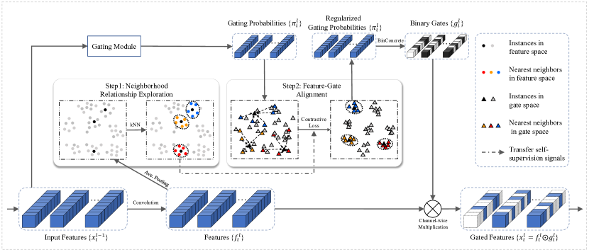
Figure 2: Flowchart of the proposed feature-gate coupling (FGC) method for dynamic network pruning. FGC consists of two iterative steps: neighborhood relationship exploration for instance-wise neighborhood relationship modeling and feature-gate alignment for gated module regularization.

Contrastive learning has been widely explored in unsupervised and self-supervised learning [30, 31, 32] to learn consistent representation. The key point is to identify similar/positive or dissimilar/negative instances. An intuitive method is taking each instance itself as positive [11]. However, its relationship with nearby instances is ignored, which is solved by exploring the neighborhood [33] or local aggregation [34]. Unsupervised clustering methods [35, 36, 37] further enlarge the positive sets by treating instances in the same cluster as positives. It is also noticed that positive instances could be gained from multiple views [38, 39] of a scene. Besides, recent methods [30, 40, 41, 42, 43] generate positive instances by siamese encoders, which process data-augmentation of original instances. The assumption is that the instance should stay close in the representation space after whatever augmentation is applied.

According to previous works, contrastive loss is an ideal tool to align distributions or learn consistent representation. Therefore, we adopt the contrastive learning method in our work, $i.e.$, the positives are deemed by neighborhood relationships, and the loss function is defined as a variant of InfoNCE [44, 45, 38].

3 Methodology

The objective of feature-gate coupling (FGC) is to align distributions of both features and gates to improve the performance of dynamic channel pruning with gating modules. To this end, we first explore instance neighborhood relationships within the feature space and transfer them to self-supervisory signals. We then propose the contrastive loss to regularize gating modules using the generated signals. In Fig. 2, we illustrate the two iterative steps, which are summarized as follows:

• Neighborhood relationship exploration: We present a $k$NN based method to explore instance neighborhood relationships in the feature space. Specifically, we adopt dot-product to evaluate similarities between feature vectors of instance pairs. The similarities are then leveraged to identify the closest instances in the feature space, denoted as nearest neighbors. Finally, indexes of those neighbors are memorized and delivered to the next step.

• Feature-gate alignment: We present a contrastive learning based method to regularize gating modules. Following indexes of neighbors in the previous step, we define these instances as positive instances in the contrastive loss function. The contrastive loss is then minimized to pull the positives together and push negatives away in the gate space.

The two steps are conducted iteratively until the optimal dynamic model is obtained. Note that FGC can be generalized to any form of gating module, although it is only tested on a popular gating module [9] in this study.

3.1 Preliminaries

We introduce the basic formulation of gated convolutional layers [9]. For an instance in the dataset $\{x_{i},y_{i}\}_{n=1}^{N}$, its feature in the $l$-th layer of CNNs is denoted as

$$x_{i}^{l}=F(x_{i}^{l-1})=ReLU(w^{l}\ast x_{i}^{l-1}).$$ (1)

where $x_{i}^{l-1}\in\mathbb{R}^{C^{l-1}\times W^{l-1}\times H^{l-1}}$ is the input of the $l$-th convolutional layer, and $x_{i}^{l}\in\mathbb{R}^{C^{l}\times W^{l}\times H^{l}}$ is the output, of which the channel number is $C^{l}$. $w^{l}$ denotes the convolutional weight matrix, $\ast$ is the convolutional operator and $ReLU$ the activation function. Batch normalization is applied after each convolution layer.

Dynamic channel pruning methods temporarily remove channels to reduce related computation in both preceding and succeeding layers, where a binary gate vector, generated from the preceding feature $x_{i}^{l-1}$, is used to turn on or turn off corresponding channels. The gated feature in the $l$-th layer is denoted as:

$$x_{i}^{l}=G(x_{i}^{l-1})\odot F(x_{i}^{l-1}),$$ (2)

where $G$ denotes the gating module and $\odot$ denotes the channel-wise multiplication.

For various basic gated modules ($G$), the basic function is uniform. Without loss of generality, we use the form of gating module [9], which is defined as

$$g_{i}^{l}=G(x_{i}^{l-1})=BinConcrete(Linear(p(x_{i}^{l-1}))).$$ (3)

The gating module first goes with the global average pooling layer $p$, which is used to generate the spatial descriptor of the input feature $x_{i}^{l-1}$. A lightweight network with two fully connected layers is then applied to generate the gating probability $\pi_{i}^{l}=Linear(p(x_{i}^{l-1}))$. Finally, activation function $BinConcrete$ [46, 47] is used to sample from $\pi_{i}^{l}$ to get the binary mask $g_{i}^{l}$.

Feature and gate of input instance are respectively denoted as $f_{i}^{l}=F(x_{i}^{l-1})$ and $g_{i}^{l}=G(x_{i}^{l-1})$ so that the gated feature is rewritten as $x_{i}^{l}=f_{i}^{l}\odot g_{i}^{l}$ (Eq. (2)).

3.2 Implementation

Neighborhood Relationship Exploration. Instance neighborhood relationships vary in different feature spaces with different semantic levels, $e.g$, in a low-level feature space, instances with similar colors or texture may be closer, while in a high-level feature space, instances in the same class may gather together. Thus, human annotations could not provide adaptive supervision of instance neighborhood relationships across different network stages. We propose to utilize the $k$NN method to adaptively explore instance neighborhood relationships in each feature space and extract self-supervisory signals accordingly for feature-gate distribution alignment.

Note that the exploration could be adopted in arbitrary layers, $e.g.$, the $l$-th layer of CNNs. In practice, in the $l$-th layer, the feature $f_{i}^{l}$ of the $i$-th instance is first flattened to a vector $\hat{f}_{i}^{l}=p(f_{i}^{l})$ using global average pooling. The dimension of pooled feature reduces from $C^{l}\times W^{l}\times H^{l}$ to $C^{l}\times 1\times 1$, which is more efficient for following processing. We then compute its similarities with other instances in the training dataset, which are measured by dot product, as

$$\mathcal{S}^{l}[i,j]=\hat{f}_{i}^{lT}\cdot\hat{f}_{j}^{l},$$ (4)

where $\mathcal{S}^{l}\in\mathbb{R}^{N\times N}$ denotes the similarity matrix and $\mathcal{S}^{l}[i,j]$ denotes similarity between the $i$-th instance and the $j$-th instance. $N$ denotes the number of total training instances. To identify nearest neighbors of $x_{i}$, we sort the $i$-th row of $\mathcal{S}_{l}$ and return the subscripts of the $k$ biggest elements, as

$$\mathcal{N}_{i}^{l}=\mathop{topk}(\mathcal{S}^{l}[i,:]).$$ (5)

The set of subscripts $\mathcal{N}_{i}^{l}$, $i.e.$, indexes of neighbor instances in the training dataset, are treated as self-supervisory signals to regularizing gating modules.

To compute the similarity matrix $\mathcal{S}^{l}$ in Eq. (4), $\hat{f}_{j}^{l}$ for all instances are required. Instead of exhaustively computing these pooled features at each iteration, we maintain a feature memory bank $\mathcal{V}_{f}^{l}\in\mathbb{R}^{N\times D}$ to store them [11]. $D$ is the dimension of the pooled feature, $i.e.$, the number of channels $C^{l}$. Now for the $i$-th pooled feature $\hat{f}_{i}^{l}$, we compute its similarities with vectors in $\mathcal{V}_{f}^{l}$. After that, the memory bank is updated in a momentum way, as

$$\mathcal{V}_{f}^{l}[i]\leftarrow m*\mathcal{V}_{f}^{l}[i]+(1-m)*\hat{f}_{i}^{l},$$ (6)

where the momentum coefficient is set to 0.5. All vectors in the memory bank are initialized as unit random vectors.

Feature-Gate Alignment. We identify the nearest neighbor set $\{x_{j},j\in\mathcal{N}_{i}^{l}\}$ of each instance $x_{i}$ in the feature space. Thereby, instances in each neighbor set are treated as positives to be pulled closer while others out of the set as negatives to be pushed away in the gate space. To this end, we utilize the contrastive loss in a self-supervised manner.

Specifically, by defining nearest neighbors of an instance as its positives, the probability of an input instance $x_{j}$ being recognized as nearest neighbors of $x_{i}$ in the gate space, as

$$p(j|\pi_{i}^{l})=\frac{exp(\pi_{j}^{lT}\cdot\pi_{i}^{l}/\tau)}{\sum_{k=1}^{N}(exp(\pi_{k}^{lT}\cdot\pi_{i}^{l})/\tau)},$$ (7)

where $\pi_{i}^{l}$ and $\pi_{j}^{l}$ are gating probabilities, the gating module outputs of $x_{i}$ and $x_{j}$ respectively. $\tau$ is a temperature hyper-parameter and set as 0.07 according to [11]. Then the loss function is derived after summing up $p(j|\pi_{i}^{l})$ of all $k$ neighbors, as

$$\mathcal{L}_{g}^{l}=-\sum_{j\in\mathcal{N}_{i}^{l}}{log(p(j|\pi_{i}^{l}))}.$$ (8)

As discussed before, the original contrastive loss [11] is minimized to gather positives and disperse negatives. Since nearest neighbors are defined as positives and others as negatives, Eq. (8) is minimized to draw previous nearest neighbors close, $i.e.$, reproducing the instance neighborhood relationships within the gate space.

Similarly, we maintain a gate memory bank $\mathcal{V}_{g}^{l}\in\mathbb{R}^{N\times D}$ to store gating probabilities. For each $\pi_{i}^{l}$, its positives are taken from $\mathcal{V}_{g}^{l}$ according to $\mathcal{N}_{i}^{l}$. After computing Eq. (8), $\mathcal{V}_{g}^{l}$ is updated in a similar momentum way as updating the feature memory bank. All vectors in $\mathcal{V}_{g}^{l}$ are initialized as unit random vectors.

Algorithm 1 Feature-Gate Coupling.

0:  Training instances $x_{i}$, labels $y_{i}$ of an imagery dataset;

0:  Dynamic network with parameters $\theta$;

1:  Initialize feature and gate memory banks $\mathcal{V}^{l}_{f}$ and $\mathcal{V}^{l}_{g}$ for layers in $\Omega$;

2:  for layer $l$ = 1 to $L$ do

3:     Generate feature $f_{i}$ and gating probability $\pi_{i}$ of instance $x_{i}$;

4:     if $l\in\Omega$ then

5:        Generate pooled feature $\hat{f}_{i}$ of instance $x_{i}$; Step 1. Neighborhood Relationship Exploration

6:        Calculate the similarities of $\hat{f}^{l}_{i}$ with $\mathcal{V}^{l}_{f}[j],(j\in(1,N),j\neq i$), (Eq.(4))

7:        Get indexes of nearest neighbors $\mathcal{N}^{l}_{i}$, (Eq.(5));

8:        Update the feature memory bank $\mathcal{V}^{l}_{f}$, (Eq.(6)); Step 2. Feature-Gate Alignment

9:        Draw positive instances w.r.t. $\mathcal{N}^{l}_{i}$ from the gate memory bank $\mathcal{V}^{l}_{g}$;

10:        Calculate the contrastive loss in the gate space $\mathcal{L}^{l}_{g}$, (Eq.(8));

11:        Update the gate memory bank $\mathcal{V}^{l}_{g}$;

12:     end if

13:     Calculate $\mathcal{L}^{l}_{0}$;

14:  end for

15:  Calculate the overall objective loss, (Eq.(9));

16:  Updating parameters $\theta$ by gradient back-propagation.

Overall Objective Loss Besides the proposed contrastive loss, we utilize the cross-entropy loss $\mathcal{L}_{ce}$ for the classification task and the l0 loss $\mathcal{L}_{0}$ to introduce sparsity. The overall loss function of our method is derived by summing these losses:

$$loss=\mathcal{L}_{ce}+\eta\cdot\sum_{l\in\Omega}\mathcal{L}_{g}^{l}+\rho\cdot\sum_{l}\mathcal{L}_{0}^{l},$$ (9)

where $\mathcal{L}_{g}^{l}$ denotes the contrastive loss adopted in the $l$-th layer and $\eta$ the corresponding coefficient. Note that $\mathcal{L}_{g}^{l}$ could be applied in arbitrary layers, e.g., a set of layers $\Omega$. $\mathcal{L}_{0}^{l}=\lVert\pi_{i}^{l}\rVert_{0}$ loss is used in each gated layer, where $\lVert\cdot\rVert_{0}$ is l0-norm. The coefficient $\rho$ controls the sparsity of pruned models, $i.e.$, a bigger $\rho$ leads to a sparser model with lower accuracy, while a lower $\rho$ derives less sparsity and higher accuracy.

The learning procedure of FGC is summarized as Algorithm 1.

3.3 Theoretical Analysis

We analyze the plausibility of the designed contrastive loss (Eq. (8)) from the perspective of mutual information maximization. According to [44], the InfoNCE loss is used to maximize the mutual information between learned representation and input signals. It is assumed that minimizing the contrastive loss leads to improved mutual information between features and corresponding gates.

Inspired by [44], we define the mutual information between gates and features as:

$$I(f^{l},g^{l})=\sum_{f^{l},g^{l}}p(f^{l},g^{l})log\frac{p(f^{l}|g^{l})}{p(f^{l})}.$$ (10)

The mutual information between $f_{j}^{l}$ and $g_{i}^{l}$ can be modeled by a density ratio $q(f_{j}^{l},g_{i}^{l})\propto p(f_{j}^{l}|g_{i}^{l})/p(f_{j}^{l})$, and in our case $q(f_{j}^{l},g_{i}^{l})=exp(\pi_{j}^{lT}\cdot\pi_{i}^{l}/\tau)$, as Eq. (7) shows. Note that $\pi_{i}^{l}$ is the gating probabilities for $g_{i}^{l}$ and $\pi_{j}^{l}$ belongs to its positives. The InfoNCE loss function is then rewritten as

$$\mathcal{L}_{g}^{l}=-\mathop{\mathbb{E}}_{X}[log\frac{q(f_{j}^{l},g_{i}^{l})}{\sum_{f_{k}^{l}\in f^{l}}q(f_{k}^{l},g_{i}^{l})}],$$ (11)

where $f_{j}^{l}$ denotes nearest neighbors in the feature space. The mutual information between $f_{j}^{l}$ and $g_{i}^{l}$ is evaluated as

$$I(f_{j}^{l},g_{i}^{l})\geq\mathop{log}(N)-\mathcal{L}_{g}^{l},$$ (12)

It indicates that minimizing the InfoNCE loss $\mathcal{L}_{g}^{l}$ maximizes a lower bound of mutual information. Accordingly, the improvement of mutual information between features and corresponding gates facilities distribution alignment. (Please refer to Fig. 10.)

4 Experiments

In this section, the experimental settings for dynamic channel pruning are first described. Ablation studies are then conducted to validate the effectiveness of FGC. The alignment of instance neighborhood relationships by the FGC is also quantitatively and qualitatively analyzed. Finally, we show the performance of learned dynamic networks on benchmark datasets and compare them with the state-of-the-art pruning methods.

4.1 Experimental Settings.

Datasets. Experiments are conducted on image classification benchmarks including CIFAR10/100 [48] and ImageNet [49]. CIFAR10 and CIFAR100 consist of 10 and 100 categories, respectively. Both datasets contain 60K colored images, 50K and 10K of which are used for training and testing. ImageNet is an important large-scale dataset composed of 1000 object categories, which has 1.28 million images for training and 50K images for validation.

Implementation Details. For CIFAR10 and CIFAR100, training images are applied with standard data augmentation schemes [50]. We use the ResNet of various depths, $i.e.$, ResNet–{20, 32, 56}, to fully demonstrate the effectiveness of our method. On CIFAR10, models are trained for 400 epochs with a mini-batch of 256. A Nesterov’s accelerated gradient descent optimizer is used, where the momentum is set to 0.9 and the weight decay is set to 5e-4. It is noticed that no weight decay is applied to parameters in gating modules. As for the learning rate, we adopt a multiple-step scheduler, where the initial value is set to 0.1 and decays by 0.1 at milestone epochs [200, 275, 350]. On CIFAR100, models are trained for 200 epochs with a mini-batch of 128. The same optimization settings as CIFAR10 are used. The initial learning rate is set to 0.1, then decays by 0.2 at epochs [60, 120, 160].

For ImageNet, the data augmentation scheme is adopted from [23]. We only use ResNet-18 to validate the effectiveness on the large-scale dataset due to time-consuming training procedures. We train models for 130 epochs with a mini-batch of 256. A similar optimizer is used except for the weight decay of 1e-4. The learning rate is initialized to 0.1 and decays by 0.1 at epochs [40, 70, 100].

FGC is employed in the last few residual blocks of ResNets, $i.e.$, last two blocks of ResNet-{20,32}, last four blocks of ResNet-56 and the last block of ResNet-18. Hyper-parameters $\eta$ and $k$ are set to 0.003 and 200 by default, respectively. We set the l0 loss coefficient $\rho$ as 0.4 to introduce considerable sparsity into gates. We conduct all experiments with PyTorch on NVIDIA RTX 3090 GPUs.

Table 1: Test errors and pruning ratios of the pruned ResNet-20 w.r.t the number of nearest neighbors $k$. ‘Error’ is the classification error, where ‘$\downarrow$’ denotes the lower the better. ‘Pruning’ is the pruning ratio of computation, where ‘$\uparrow$’ denotes the higher the better. (Ditto for other tables.)

$K$	5	20	100	200	512	1024	2048	4096
Error (%) $\downarrow$	8.47	8.01	8.00	7.91	8.16	8.04	8.09	8.39
Pruning (%) $\uparrow$	50.1	54.1	53.4	55.1	53.3	54.9	53.0	53.8

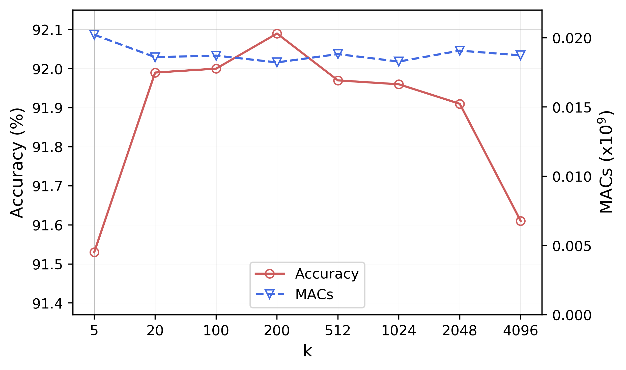
Figure 3: Test accuracies and computation of the pruned ResNet-20 w.r.t the number of nearest neighbors $k$.

4.2 Ablation study

We conduct ablation studies on CIFAR10 to validate the effectiveness of our method by exploring hyper-parameters, residual blocks, neighborhood relationships, and accuracy-computation trade-off.

Hyper-parameters of Contrastive Loss. In Table 1 and Fig. 3, we show the performance of pruned models given different $k$, $i.e.$, the number of nearest neighbors. For a fair comparison, the computation of each model is tuned to be roughly the same so that it could be evaluated by accuracy. As shown by Fig. 3, FGC is robust about $k$ in a wide range, $i.e.$, the accuracy reaches the highest value around $k=$200, and keeps stable when $k$ falls into the range (20, 1024). It is noticed that the accuracy is low when $k=5$ or $k=4096$, $i.e.$, either too few or too many neighbors involved. We argue that few neighbors fail to capture the local relationships while superfluous neighbors may bring global information that disturbs the local ones.

In Table 2 and Fig. 4, we show the performance of pruned models under different $\eta$, $i.e.$, the loss coefficient. Similarly, the computation of each model is also tuned to be almost the same. The contrastive loss brings a significant accuracy improvement compared with models without FGC. With the increase of $\eta$, the accuracy improves from 91.4% to 92.09%. The best performance is achieved when $\eta=0.003$. While accuracy slightly drops when $\eta$ is larger than 0.01, it remains better than that at $\eta=0$.

Table 2: Test errors and pruning ratios of the pruned ResNet-20 w.r.t coefficient $\eta$.

$\eta$	0	5e-4	0.001	0.002	0.003	0.005	0.01	0.02
Error (%) $\downarrow$	8.59	8.47	8.22	8.12	7.91	7.94	8.01	8.21
Pruning (%) $\uparrow$	54.0	54.8	53.2	55.3	55.1	53.1	53.0	52.4

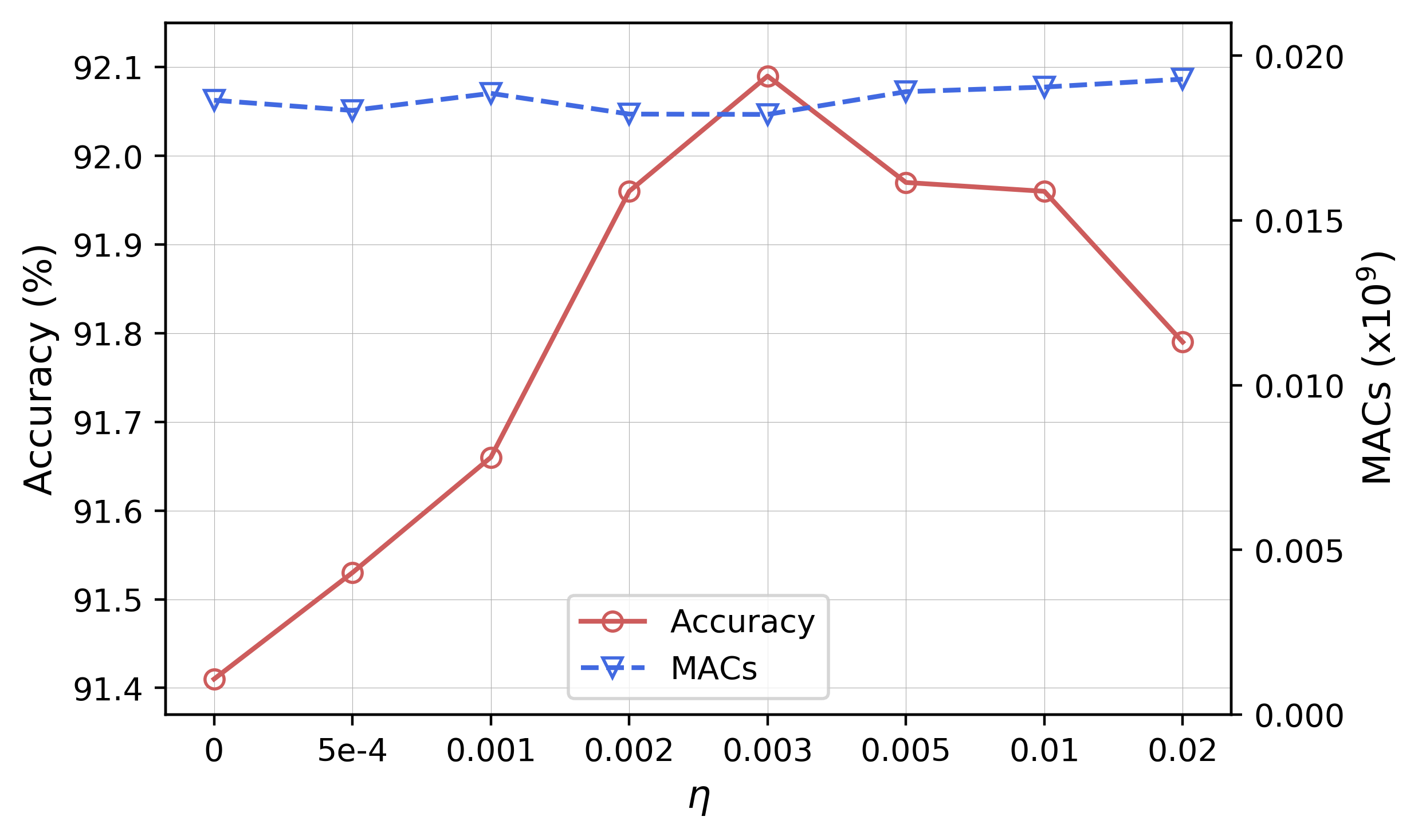
Figure 4: Test accuracies and computation of the pruned ResNet-20 w.r.t coefficient $\eta$.

Residual Blocks. In Table 3, we exploit whether FGC is more effective when employed in multiple residual blocks. The first row of Table 3 denotes models trained without FGC. After gradually removing shallow residual blocks from adopting FGC, experimental results show that FGC in shallow stages brings a limited performance gain despite more memory banks, $e.g.$, total $18$ memory banks used when employing FGC in all blocks. However, FGC in the last stage, especially from the $8$-$th$ to the $9$-$th$ blocks, contributes better to the final performance, $i.e.$, the lowest error (7.91%) with considerable computation reduction (55.1%). It is concluded that the residual blocks in deep stages benefit more from FGC, probably due to more discriminative features and more conditional gates. Therefore, taking both training efficiency and performance into consideration, we employ FGC in the deep stages of ResNets.

Table 3: Test errors and pruning ratios of pruned ResNet-20 when employing FGC in different blocks.

Stages	Blocks	Memory Banks	Error (%) $\downarrow$	Pruning (%) $\uparrow$
-	-	-	8.49	54.3
$1^{st}$ to $3^{rd}$	$1^{st}$ to $9^{th}$	18	8.08	53.4
$2^{nd}$ to $3^{rd}$	$4^{th}$ to $9^{th}$	12	8.36	56.0
$3^{rd}$	$7^{th}$ to $9^{th}$	6	8.21	56.0
	$8^{th}$ to $9^{th}$	4	7.91	55.1
	Only $9^{th}$	2	8.14	54.5

Neighborhood Relationship Sources. In Table 4, we validate the necessity of exploring instance neighborhood relationships in feature spaces by comparing the counterparts. Specifically, we randomly select $k$ instances with the same label as neighbors for each input instance, denoted as ‘Label’; we also utilize $k$NN in the gate space to generate nearest neighbors, denoted as ‘Gate’. Moreover, since FGC is applied in multiple layers separately, an alternative adopts neighborhood relationships from the same layer, $e.g.$, the last layer. We define this case as ‘Feature’ with ‘Shared’ instance neighborhood relationships.

Results in Table 4 demonstrate that our method, $i.e.$, ‘Feature’ with independent neighbors, prevails all the counterparts, which fail to explore proper instance neighborhood relationships for alignment. For example, labels are too coarse or discrete to describe instance neighborhood relationships. Exploring neighbors in the gate space enhances its misalignment with the feature space. Therefore the performance, either error or pruning ratio (8.50%, 51.6%), is even worse than the model without FGC. Moreover, ‘Shared’ neighbors from the same feature space could not deal with variants of intermediate features, thereby the improvement of which is limited.

We conclude that the proposed FGC method consistently outperforms the compared methods, which attributes to the alignment of instance neighborhood relationships between feature and gate spaces in multiple layers.

Table 4: Comparison of utilizing various methods to explore instance neighborhood relationships. (ResNet-20)

Neighbors Source	Shared	Error (%) $\downarrow$	Pruning (%) $\uparrow$
-	-	8.49	54.3
Label	✗	8.16	52.0
Gate	✗	8.50	51.6
Feature	✓	8.14	51.2
Feature	✗	7.91	55.1

Computation-Accuracy Trade-off. In Fig. 5, we show the computation-accuracy trade-off points of the proposed method and the baseline method by selecting $\mathcal{L}_{0}$ loss coefficient $\rho$ from values of {0.01, 0.02, 0.05, 0.1, 0.2, 0.4}. Experimental results on ResNet-{20, 32} show that the accuracy of pruning models increases as the total computational cost increases. Compared with pruned models without FGC, the pruned ResNet-32 with FGC obtains higher accuracy with lower computational cost, as shown in the top right of Fig. 5. At the left bottom of Fig. 5, the pruned ResNet-20 with FGC achieves  $0.5\%$ higher accuracy using the same computational cost. Note that an increased performance compared with the baseline models is observed at a lower ‘pruning ratio’, which is common in pruning methods due to extra regularization [51]. We conclude that the pruned models by our FGC method consistently outperform those by the baseline method.

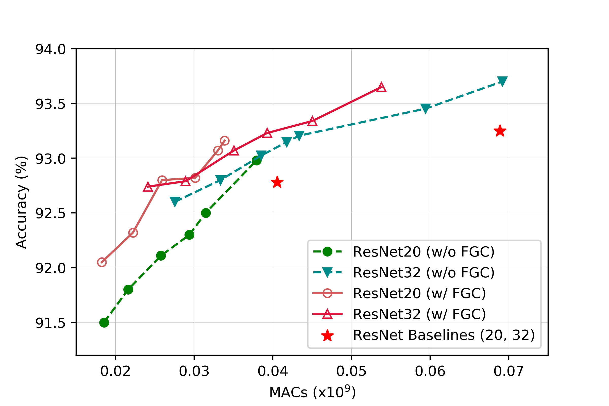
Figure 5: Computation-Accuracy trade-off of pruned ResNet-{20, 32} with or without FGC.

4.3 Analysis

Visualization Analysis. In Fig. 6, we use UMAP [52] to visualize the correspondence of features and gates during the training procedure. Specifically, we show features and gates from the last residual block (conv3-3) of ResNet-20, where features are trained to be discriminative, $i.e.$, easy to be distinguished in the embedding space. It’s seen that features and gates are simultaneously optimized and evolve together as the training epoch increases. In the last epoch, as instance neighborhood relationships been well reproduced in the gate space, we can observe gates with similar discrimination as features, $e.g.$, instances of same clusters in the feature space are also assembled in the gate space. Intuitively, the coupling of features and gates promises gated features with consistent discrimination, which justifies the better prediction of our pruned models with given pruning ratios.

In Fig. 7, we further compare feature and gate embeddings with pruned models in BAS [9]. Specifically, features and gates are drawn from the last residual block (conv3-3) of ResNet-20 and the second to last residual block (conv3-4) of ResNet-32. As shown, our method brings pruned models with coupled features and gates, compared with BAS. For example, ‘bird’ (green), ‘frog’ (grey) and ‘deer’ (brown) instances entangle together (left bottom of Fig. 7a), while they are clearly distinguished as corresponding features after adopting FGC (right bottom of Fig. 7a). Similar observations are seen in Fig. 7b, validating the effect of FGC.

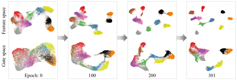
Figure 6: Embedding visualization of features and gates in ResNet-20 (conv3-3) trained with FGC at different training epochs. Each point denotes an instance in the dataset (CIFAR10). Each color denotes one category. (Best view in color).

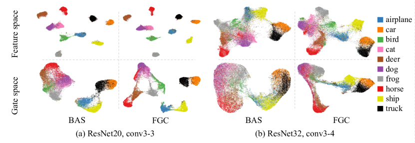
Figure 7: Embedding visualization of features and gates in pruned models trained with FGC, compared with pruned models in BAS [9]. (Best view in color).

In Fig. 8, we visualize the execution frequency of channels in pruned ResNet-20 for each category on CIFAR10. Especially in shallow layers ($e.g.$, conv1-3), gates are almost entirely turn on or off for arbitrary categories, indicating why FGC is unnecessary: a common channel compression scheme is enough. However, in deep layers ($e.g.$, conv3-3), dynamic pruning is performed according to the semantics of categories. It’s noticed that semantically similar categories, such as ‘dog’ and ‘cat’, also share similar gate execution patterns. We conclude that FGC utilizes and enhances the correlation between instance semantics and pruning patterns to pursue better representation.

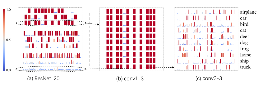
Figure 8: Execution frequency of channels in pruned models. The color and height of each bar denote the value of execution frequency. (a) Execution frequency in each layer listed from top to bottom. (b) Execution frequency of each category in conv1-3. (c) Execution frequency of each category in conv3-3.

In Fig. 9, we show images in the ordering of gate similarities with the target ones (leftmost). One can see that the semantic similarities and gate similarities of image instances decrease consistently from left to right.

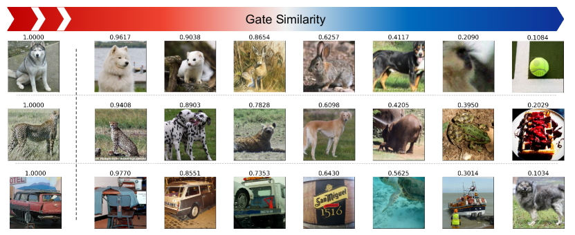
Figure 9: Sorted images w.r.t gates similarities on ImageNet validation set. In each row, we list example images according to their gate similarities (values above images) with the leftmost one. Gates are drawn from the $8$-$th$ gated block of ResNet-18.

Mutual Information Analysis. In Fig. 10, we validate that FGC improves the mutual information between features and gates to facility distribution alignment, as discussed in section 3.3. For comparison, only partial deep layers are employed with FGC in our pruned models, indicated by ‘$\ast$’. Specifically, for layers not employed with FGC, the normalized mutual information (NMI) between features and gates is roughly unchanged. However, for layers employed with FGC, we observe the consistent improvement of NMI between features and gates, compared with the pruned models in BAS [9].

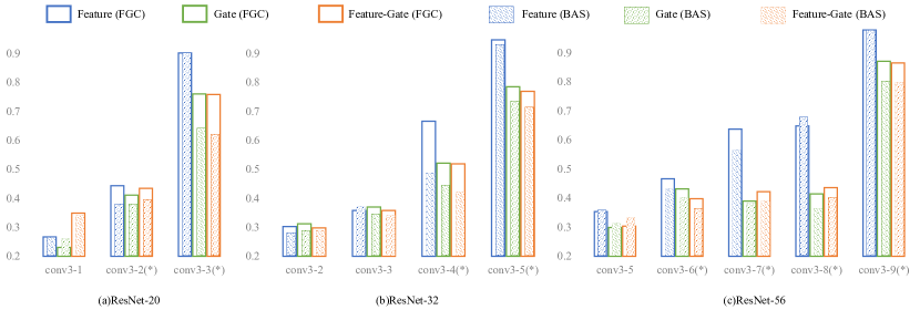
Figure 10: Normalized mutual information (NMI) in deep residual blocks of ResNet-{20, 32, 56}, compared with pruned models in BAS [9]. ‘Feature’ denotes NMI between features and labels; ‘Gate’ denotes NMI between gates and labels; ‘Feature-Gate’ denotes NMI between features and gates. ‘$\ast$’ denotes residual blocks employed with FGC.

4.4 Performance

We compare the proposed method with the state-of-the-art methods, including both static and dynamic methods. The performance is evaluated by two metrics, classification errors and average pruning ratios of computation. Higher pruning ratios and lower errors indicate better pruned models.

CIFAR10. In Table 5, comparison with SOTA methods to prune ResNet-{20, 32, 56} is shown. FGC significantly outperforms static pruning methods. For ResNet-20, models trained with FGC reduce $57.4\%$ computation, $11.9\%$ more than Hinge [13], given a rather similar accuracy ($8.13\%$ $vs$ $8.16\%$). It also prevails other dynamic pruning methods, $i.e.$, least classification error ($7.91\%$) with more reduction of computational cost ($55.1\%$). Our pruned ResNet-34 and ResNet-56 achieve the least classification errors ($7.26\%$ and $6.09\%$ respectively) with significant pruning ratios and the highest pruning ratios ($66.9\%$ and $66.2\%$ respectively) with limited accuracy degradation. We can conclude that FGC consistently outperforms other pruning methods despite various architectures.

Table 5: Comparison of the pruned ResNet with different methods on CIFAR-10.

Model	Method	Dynamic	Error (%) $\downarrow$	Pruning (%) $\uparrow$
ResNet-20	Baseline	-	7.22	0.0
	SFP [4]	✗	9.17	42.2
	FPGM [5]	✗	9.56	54.0
	DSA [12]	✗	8.62	50.3
	Hinge [13]	✗	8.16	45.5
	DHP [14]	✗	8.46	51.8
	FBS [8]	✓	9.03	53.1
	BAS [9]	✓	8.49	54.3
	FGC (Ours)	✓	7.91	55.1
	FGC (Ours)	✓	8.13	57.4
ResNet-32	Baseline	-	6.75	0.0
	SFP [4]	✗	7.92	41.5
	FPGM [5]	✗	8.07	53.2
	FBS [8]	✓	8.02	55.7
	BAS [9]	✓	7.79	64.2
	FGC (Ours)	✓	7.26	65.0
	FGC (Ours)	✓	7.43	66.9
ResNet-56	Baseline	-	5.86	0.0
	SFP [4]	✗	7.74	52.6
	FPGM [5]	✗	6.51	52.6
	HRank [53]	✗	6.83	50.0
	DSA [12]	✗	7.09	52.2
	Hinge [13]	✗	6.31	50.0
	DHP [14]	✗	6.42	50.9
	FBS [8]	✓	6.48	53.6
	BAS [9]	✓	6.43	62.9
	FGC (Ours)	✓	6.09	62.2
	FGC (Ours)	✓	6.41	66.2

Table 6: Comparison of the pruned ResNet with different methods on CIFAR100.

Model	Method	Dynamic	Error (%) $\downarrow$	Pruning (%) $\uparrow$
ResNet-20	Baseline	-	31.38	0.0
	BAS [9]	✓	31.98	26.2
	FGC (Ours)	✓	31.37	26.9
	FGC (Ours)	✓	31.69	31.9
ResNet-32	Baseline	-	29.85	0.0
	CAC [54]	✗	30.49	30.1
	BAS [9]	✓	30.03	39.7
	FGC (Ours)	✓	29.90	40.4
	FGC (Ours)	✓	30.09	45.1
ResNet-56	Baseline	-	28.44	0.0
	CAC [54]	✗	28.69	30.0
	BAS [9]	✓	28.37	37.1
	FGC (Ours)	✓	27.87	38.1
	FGC (Ours)	✓	28.00	40.7

CIFAR100. In Table 6, we present the pruning results of ResNet-{20, 32, 56}. For example, after pruning $26.9\%$ computational cost of ResNet-20, FGC even achieves $0.01\%$ less classification error. For ResNet-32 and ResNet-56, FGC outperforms SOTA methods CAC [54] and BAS [9] with significant margins, from perspectives of both test error and computation reduction. Specifically, FGC, compared with BAS, reduces $5.4\%$ and $3.6\%$ more computation of ResNet-32 and ResNet-56 without bringing more errors. Experimental results on CIFAR100 justify the generality of our method to various datasets.

Table 7: Comparison of the pruned ResNet with different methods on ImageNet.

Model	Method	Dynamic	Top-1 Error (%) $\downarrow$	Top-5 Error (%) $\downarrow$	Pruning (%) $\uparrow$
ResNet-18	Baseline	-	30.15	10.92	0.0
	SFP [4]	✗	32.90	12.22	41.8
	FPGM [5]	✗	31.59	11.52	41.8
	PFP [55]	✗	34.35	13.25	43.1
	DSA [12]	✗	31.39	11.65	40.0
	LCCN [17]	✓	33.67	13.06	34.6
	CGNet [18]	✓	31.70	-	50.7
	FBS [8]	✓	31.83	11.78	49.5
	BAS [9]	✓	31.66	-	47.1
	FGC (Ours)	✓	30.67	11.07	42.2
	FGC (Ours)	✓	31.49	11.62	48.1

ImageNet. In Table 7, we compare our method with various SOTA methods by pruning ResNet-18. One can see that FGC outperforms most static pruning methods. For example, FPGM [5] reduces $41.8\%$ computation with $31.59\%$ top-1 error, while FGC reduces $42.2\%$ computation with $30.67\%$ top-1 error. It’s also comparable with other dynamic pruning methods. For example, compared with BAS [9], FGC prunes more computation ($48.1\%$ $vs$ $47.1\%$) with less top-1 error ($31.49\%$ $vs$ $31.66\%$). Experimental results demonstrate the effectiveness of our FGC method on the large-scale image dataset.

5 Conclusions

We propose a feature-gate coupling (FGC) method to reduce the distortion of gated features by regularizing the consistency between distributions of features and gates. FGC takes the instance neighborhood relationships in the feature space as the objective while pursuing the instance distribution coupling of the gate space by aligning instance neighborhood relationships in the feature and gate spaces. FGC utilizes the $k$-Nearest Neighbor method to explore the instance neighborhood relationships in the feature space and utilizes contrastive learning to regularize gating modules with the generated self-supervisory signals. Experimental results validate that FGC improves the performance of dynamic network pruning with striking contrast with the state-of-the-arts. FGC provides fresh insight into the network pruning problem.

References

- [1] S. Han, H. Mao, W. J. Dally, Deep compression: Compressing deep neural network with pruning, trained quantization and huffman coding, in: Proceedings of International Conference on Learning Representations (ICLR), 2016.
- [2] Y. He, X. Zhang, J. Sun, Channel pruning for accelerating very deep neural networks, in: Proceedings of International Conference on Computer Vision (ICCV), 2017, pp. 1398–1406.
- [3] P. Molchanov, S. Tyree, T. Karras, T. Aila, J. Kautz, Pruning convolutional neural networks for resource efficient inference, in: Proceedings of International Conference on Learning Representations (ICLR), 2017.
- [4] Y. He, G. Kang, X. Dong, Y. Fu, Y. Yang, Soft filter pruning for accelerating deep convolutional neural networks, in: Proceedings of International Joint Conference on Artificial Intelligence (IJCAI), 2018, pp. 2234–2240.
- [5] Y. He, P. Liu, Z. Wang, Z. Hu, Y. Yang, Filter pruning via geometric median for deep convolutional neural networks acceleration, in: Proceedings of IEEE Conference on Computer Vision and Pattern Recognition (CVPR), 2019, pp. 4340–4349.
- [6] N. Shazeer, A. Mirhoseini, K. Maziarz, A. Davis, Q. V. Le, G. E. Hinton, J. Dean, Outrageously large neural networks: The sparsely-gated mixture-of-experts layer, in: Proceedings of International Conference on Learning Representations (ICLR), 2017.
- [7] Z. Wu, T. Nagarajan, A. Kumar, S. Rennie, L. S. Davis, K. Grauman, R. S. Feris, Blockdrop: Dynamic inference paths in residual networks, in: Proceedings of IEEE Conference on Computer Vision and Pattern Recognition (CVPR), 2018, pp. 8817–8826.
- [8] X. Gao, Y. Zhao, L. Dudziak, R. D. Mullins, C. Xu, Dynamic channel pruning: Feature boosting and suppression, in: Proceedings of International Conference on Learning Representations (ICLR), 2019.
- [9] B. Ehteshami Bejnordi, T. Blankevoort, M. Welling, Batch-shaping for learning conditional channel gated networks, in: Proceedings of International Conference on Learning Representations (ICLR), 2020.
- [10] Y. Wang, X. Zhang, X. Hu, B. Zhang, H. Su, Dynamic network pruning with interpretable layerwise channel selection, in: Proceedings of AAAI Conference on Artificial Intelligence (AAAI), 2020, pp. 6299–6306.
- [11] Z. Wu, Y. Xiong, S. X. Yu, D. Lin, Unsupervised feature learning via non-parametric instance discrimination, in: Proceedings of IEEE Conference on Computer Vision and Pattern Recognition (CVPR), 2018, pp. 3733–3742.
- [12] X. Ning, T. Zhao, W. Li, P. Lei, Y. Wang, H. Yang, DSA: more efficient budgeted pruning via differentiable sparsity allocation, in: Proceedings of European Conference on Computer Vision (ECCV), 2020, pp. 592–607.
- [13] Y. Li, S. Gu, C. Mayer, L. V. Gool, R. Timofte, Group sparsity: The hinge between filter pruning and decomposition for network compression, in: Proceedings of IEEE Conference on Computer Vision and Pattern Recognition (CVPR), 2020, pp. 8015–8024.
- [14] Y. Li, S. Gu, K. Zhang, L. V. Gool, R. Timofte, DHP: differentiable meta pruning via hypernetworks, in: Proceedings of European Conference on Computer Vision (ECCV), 2020, pp. 608–624.
- [15] Y. Han, G. Huang, S. Song, L. Yang, H. Wang, Y. Wang, Dynamic neural networks: A survey, arXiv preprint arXiv:2102.04906.
- [16] M. Figurnov, M. D. Collins, Y. Zhu, L. Zhang, J. Huang, D. P. Vetrov, R. Salakhutdinov, Spatially adaptive computation time for residual networks, in: Proceedings of IEEE Conference on Computer Vision and Pattern Recognition (CVPR), 2017, pp. 1790–1799.
- [17] X. Dong, J. Huang, Y. Yang, S. Yan, More is less: A more complicated network with less inference complexity, in: Proceedings of IEEE Conference on Computer Vision and Pattern Recognition (CVPR), 2017, pp. 1895–1903.
- [18] W. Hua, Y. Zhou, C. D. Sa, Z. Zhang, G. E. Suh, Channel gating neural networks, in: Proceedings of Advances in Neural Information Processing Systems (NeurIPS), 2019, pp. 1884–1894.
- [19] Z. Xie, Z. Zhang, X. Zhu, G. Huang, S. Lin, Spatially adaptive inference with stochastic feature sampling and interpolation, in: Proceedings of European Conference on Computer Vision (ECCV), 2020, pp. 531–548.
- [20] S. Teerapittayanon, B. McDanel, H. T. Kung, Branchynet: Fast inference via early exiting from deep neural networks, in: Proceedings of International Conference on Pattern Recognition (ICPR), 2016, pp. 2464–2469.
- [21] G. Huang, D. Chen, T. Li, F. Wu, L. van der Maaten, K. Q. Weinberger, Multi-scale dense networks for resource efficient image classification, in: Proceedings of International Conference on Learning Representations (ICLR), 2018.
- [22] T. Bolukbasi, J. Wang, O. Dekel, V. Saligrama, Adaptive neural networks for efficient inference, in: Proceedings of International Conference on Machine Learning (ICML), 2017, pp. 527–536.
- [23] K. He, X. Zhang, S. Ren, J. Sun, Deep residual learning for image recognition, in: Proceedings of IEEE Conference on Computer Vision and Pattern Recognition (CVPR), 2016, pp. 770–778.
- [24] X. Wang, F. Yu, Z. Dou, T. Darrell, J. E. Gonzalez, Skipnet: Learning dynamic routing in convolutional networks, in: Proceedings of European Conference on Computer Vision (ECCV), 2018, pp. 420–436.
- [25] A. Veit, S. J. Belongie, Convolutional networks with adaptive inference graphs, in: Proceedings of European Conference on Computer Vision (ECCV), 2018, pp. 3–18.
- [26] J. Lin, Y. Rao, J. Lu, J. Zhou, Runtime neural pruning, in: Proceedings of Advances in Neural Information Processing Systems (NeurIPS), 2017, pp. 2181–2191.
- [27] C. Ahn, E. Kim, S. Oh, Deep elastic networks with model selection for multi-task learning, in: Proceedings of International Conference on Computer Vision (ICCV), 2019, pp. 6528–6537.
- [28] A. E. Bejnordi, R. Krestel, Dynamic channel and layer gating in convolutional neural networks, in: (KI), 2020, pp. 33–45.
- [29] R. Hadsell, S. Chopra, Y. LeCun, Dimensionality reduction by learning an invariant mapping, in: Proceedings of IEEE Conference on Computer Vision and Pattern Recognition (CVPR), 2006, pp. 1735–1742.
- [30] J. Grill, F. Strub, F. Altché, C. Tallec, P. H. Richemond, E. Buchatskaya, C. Doersch, B. Á. Pires, Z. Guo, M. G. Azar, B. Piot, K. Kavukcuoglu, R. Munos, M. Valko, Bootstrap your own latent - A new approach to self-supervised learning, in: Proceedings of Advances in Neural Information Processing Systems (NeurIPS), 2020.
- [31] D. Luo, C. Liu, Y. Zhou, D. Yang, C. Ma, Q. Ye, W. Wang, Video cloze procedure for self-supervised spatio-temporal learning, in: Proceedings of AAAI Conference on Artificial Intelligence (AAAI), 2020, pp. 11701–11708.
- [32] Y. Yao, C. Liu, D. Luo, Y. Zhou, Q. Ye, Video playback rate perception for self-supervised spatio-temporal representation learning, in: Proceedings of IEEE Conference on Computer Vision and Pattern Recognition (CVPR), 2020, pp. 6547–6556.
- [33] J. Huang, Q. Dong, S. Gong, X. Zhu, Unsupervised deep learning by neighbourhood discovery, in: Proceedings of International Conference on Machine Learning (ICML), 2019, pp. 2849–2858.
- [34] C. Zhuang, A. L. Zhai, D. Yamins, Local aggregation for unsupervised learning of visual embeddings, in: Proceedings of International Conference on Computer Vision (ICCV), 2019, pp. 6001–6011.
- [35] Y. Zhang, C. Liu, Y. Zhou, W. Wang, W. Wang, Q. Ye, Progressive cluster purification for unsupervised feature learning, in: Proceedings of International Conference on Pattern Recognition (ICPR), 2020, pp. 8476–8483.
- [36] M. Caron, I. Misra, J. Mairal, P. Goyal, P. Bojanowski, A. Joulin, Unsupervised learning of visual features by contrasting cluster assignments, in: Proceedings of Advances in Neural Information Processing Systems (NeurIPS), 2020.
- [37] J. Huang, S. Gong, Deep clustering by semantic contrastive learning, arXiv preprint arXiv:2103.02662.
- [38] P. Bachman, R. D. Hjelm, W. Buchwalter, Learning representations by maximizing mutual information across views, in: Proceedings of Advances in Neural Information Processing Systems (NeurIPS), 2019, pp. 15509–15519.
- [39] Y. Tian, D. Krishnan, P. Isola, Contrastive multiview coding, in: Proceedings of European Conference on Computer Vision (ECCV), 2020, pp. 776–794.
- [40] X. Chen, K. He, Exploring simple siamese representation learning, arXiv preprint arXiv:2011.10566.
- [41] T. Chen, S. Kornblith, M. Norouzi, G. E. Hinton, A simple framework for contrastive learning of visual representations, in: Proceedings of International Conference on Machine Learning (ICML), 2020, pp. 1597–1607.
- [42] O. J. Hénaff, Data-efficient image recognition with contrastive predictive coding, in: Proceedings of International Conference on Machine Learning (ICML), 2020, pp. 4182–4192.
- [43] K. He, H. Fan, Y. Wu, S. Xie, R. B. Girshick, Momentum contrast for unsupervised visual representation learning, in: Proceedings of IEEE Conference on Computer Vision and Pattern Recognition (CVPR), 2020, pp. 9726–9735.
- [44] A. van den Oord, Y. Li, O. Vinyals, Representation learning with contrastive predictive coding, arXiv preprint arXiv:1807.03748.
- [45] R. D. Hjelm, A. Fedorov, S. Lavoie-Marchildon, K. Grewal, P. Bachman, A. Trischler, Y. Bengio, Learning deep representations by mutual information estimation and maximization, in: Proceedings of International Conference on Learning Representations (ICLR), 2019.
- [46] E. Jang, S. Gu, B. Poole, Categorical reparameterization with gumbel-softmax, in: Proceedings of International Conference on Learning Representations (ICLR), 2017.
- [47] C. J. Maddison, A. Mnih, Y. W. Teh, The concrete distribution: A continuous relaxation of discrete random variables, in: Proceedings of International Conference on Learning Representations (ICLR), 2017.
- [48] A. Krizhevsky, G. Hinton, Learning multiple layers of features from tiny images, 2009.
- [49] J. Deng, W. Dong, R. Socher, L. Li, K. Li, F. Li, Imagenet: A large-scale hierarchical image database, in: Proceedings of IEEE Conference on Computer Vision and Pattern Recognition (CVPR), 2009, pp. 248–255.
- [50] M. Lin, Q. Chen, S. Yan, Network in network, in: Proceedings of International Conference on Learning Representations (ICLR), 2014.
- [51] J. Frankle, M. Carbin, The lottery ticket hypothesis: Finding sparse, trainable neural networks, in: Proceedings of International Conference on Learning Representations (ICLR), 2019.
- [52] L. McInnes, J. Healy, UMAP: uniform manifold approximation and projection for dimension reduction, arXiv preprint arXiv:1802.03426.
- [53] M. Lin, R. Ji, Y. Wang, Y. Zhang, B. Zhang, Y. Tian, L. Shao, Hrank: Filter pruning using high-rank feature map, in: Proceedings of IEEE Conference on Computer Vision and Pattern Recognition (CVPR), 2020, pp. 1526–1535.
- [54] Z. Chen, T. Xu, C. Du, C. Liu, H. He, Dynamical channel pruning by conditional accuracy change for deep neural networks, IEEE Trans. Neural Networks Learn. Syst. (TNNLS) 32 (2) (2021) 799–813.
- [55] L. Liebenwein, C. Baykal, H. Lang, D. Feldman, D. Rus, Provable filter pruning for efficient neural networks, in: Proceedings of International Conference on Learning Representations (ICLR), 2020.