Localization of space-inhomogeneous
three-state quantum walks

Abstract

Mathematical analysis on the existence of eigenvalues is essential because it is equivalent to the occurrence of localization, which is an exceptionally crucial property of quantum walks. We construct the method for the eigenvalue problem via the transfer matrix for space-inhomogeneous $n$-state quantum walks in one dimension with $n-2$ self-loops, which is an extension of the technique in a previous study (Quantum Inf. Process 20(5), 2021). This method reveals the necessary and sufficient condition for the eigenvalue problem of a two-phase three-state quantum walk with one defect whose time evolution varies in the negative part, positive part, and at the origin.

1 Introduction

The research on quantum walks (QWs) began in the early 2000s [1, 2], and QWs play important roles in various fields, and a variety of QW models have been analyzed theoretically and numerically. This paper focuses on the mathematical analysis of discrete-time three-state QWs on the integer lattice, studied intensively by [3, 4, 5, 6, 7, 8, 9]. Three-state QWs have an interesting property called localization, where the probability of finding the particle around the initial position remains positive in the long-time limit. Localization on multi-state (three or more states) QWs is actively researched by previous studies [10, 11, 12, 13, 14, 15, 16]. In the research of multi-state QWs, the Grover walk, whose time evolution is defined by the Grover matrix as a coin matrix, often plays an essential role. The name comes from Grover’s search algorithm [17]. Two-phase two-state QWs with one defect whose time evolution varies in the negative part, positive part, and at the origin are also investigated intensively [18, 19, 20, 21, 22, 23, 24, 25]. This model contains one-defect QWs where the walker at the origin behaves differently and two-phase QWs where the walker behaves differently in each negative and non-negative part. Localization on one-defect Grover walk is applied for quantum search algorithms [26, 27, 28], which are expected to generalize Grover’s algorithm and speed up the search algorithms on general graphs. Also, localization on two-phase QW is related to the research of topological insulators [29, 20].

The QW model exhibits localization if and only if there exists an eigenvalue of the time evolution operator, and the amount of localization is deeply related to its corresponding eigenvector and the initial state of the model [30]. Solving the eigenvalue problem via the transfer matrix was constructed for two-phase two-state QWs with one defect in [25] and for more general space-inhomogeneous QWs in [31]. The transfer matrix is also used in [32, 33, 34]. In this paper, we extend the transfer matrix method to $n$-state QWs with $n-2$ self-loops. Furthermore, we apply the techniques to two-phase three-state QWs with one defect defined by the generalized Grover matrix.

The rest of this paper is organized as follows. In Section 2, we define $n$-state QWs with $n-2$ self-loops, which is an extension of three-state QWs on the integer lattice. Then, we give the transfer matrix in a general way and construct methods for the eigenvalue problem. Theorem 2.3 is the main theorem, which gives a necessary and sufficient condition for the eigenvalue problem. Section 3 focuses on the concrete calculation of eigenvalues on one-defect and two-phase three-state QWs with generalized Grover coin matrices. We also show some figures indicating eigenvalues of the time evolution operators and their corresponding probability distributions in this section.

2 Definitions and Method

2.1 Multi-state quantum walks on the integer lattice

Firstly, we introduce $n$-state QWs with $n-2$ self-loops on the integer lattice $\mathbb{Z}$. Let $\mathcal{H}$ be a Hilbert space defined by

$$\mathcal{H}=\ell^{2}(\mathbb{Z};\mathbb{C}^{n})=\left\{\Psi:\mathbb{Z}\to\mathbb{C}^{n}\ \middle|\ \sum_{x\in\mathbb{Z}}\|\Psi(x)\|_{\mathbb{C}^{n}}^{2}<\infty\right\},$$

where $n\geq 3$ and $\mathbb{C}$ denotes the set of complex numbers. We write $n$-state quantum state $\Psi:\mathbb{Z}\rightarrow\mathbb{C}^{n}$ as below:

$$\Psi(x)=\left[\begin{array}[]{ c }\Psi_{1}(x)\\ \Psi_{2}(x)\\ \vdots\\ \Psi_{n}(x)\end{array}\right].$$

Let $\{C_{x}\}_{x\in\mathbb{Z}}$ be a sequence of $n\times n$ unitary matrices, which is written as below:

$$C_{x}=e^{i\Delta_{x}}\left[\begin{array}[]{ c c c c }a_{x}^{(1,1)}&a_{x}^{(1,2)}&\dotsc&a_{x}^{(1,n)}\\ a_{x}^{(2,1)}&a_{x}^{(2,2)}&\dotsc&a_{x}^{(2,n)}\\ \vdots&\vdots&\ddots&\vdots\\ a_{x}^{(n,1)}&a_{x}^{(n,2)}&\dotsc&a_{x}^{(n,n)}\end{array}\right].$$

where $\Delta_{x}\in[0,2\pi),\ a^{(j,k)}_{x}\in\mathbb{C},(1\leq j,k\leq n)$ and $|a^{(k,k)}_{x}|\neq 1\ (2\leq k\leq n-1)$. Here we define $C_{x}$ with additional phases $\Delta_{x}$ for the simplification of the discussion in Subsection 2.2. Then the coin operator $C$ on $\mathcal{H}$ is given as

$$(C\Psi)=C_{x}\Psi(x).$$

The shift operator $S$ is also an operator on $\mathcal{H}$, which shifts $\Psi_{1}(x)$ and $\Psi_{n}(x)$ to $\Psi_{1}(x-1)$ and $\Psi_{n}(x+1)$, respectively and does not move $\Psi_{k}(x)$ for $2\leq k\leq n-1$.

$$(S\Psi)(x)=\left[\begin{array}[]{ c }\Psi_{1}(x+1)\\ \Psi_{2}(x)\\ \vdots\\ \Psi_{k}(x)\\ \vdots\\ \Psi_{n-1}(x)\\ \Psi_{n}(x-1)\end{array}\right],\qquad 2\leq k\leq n-1.\$$

Then the time evolution operator is given as

$$U=SC.$$

We treat the model whose coin matrices satisfy

$$C_{x}=\begin{cases}C_{\infty},\quad&x\in[x_{+},\infty),\\ C_{-\infty},\quad&x\in(-\infty,x_{-}].\end{cases}$$

where $x_{+}>0,\ x_{-}<0$. For initial state $\Psi_{0}\in\mathcal{H}\ (\|\Psi_{0}\|_{\mathcal{H}}^{2}=1)$, the finding probability of a walker in position $x$ at time $t\in\mathbb{Z}_{\geq 0}$ is defined by

$$\mu_{t}^{(\Psi_{0})}(x)=\|(U^{t}\Psi_{0})(x)\|_{\mathbb{C}^{n}}^{2},$$

where $\mathbb{Z}_{\geq 0}$ is the set of non-negative integers. We say that the QW exhibits localization if there exists a position $x_{0}\in\mathbb{Z}$ and an initial state $\Psi_{0}\in\mathcal{H}$ satisfying $\limsup_{t\to\infty}\mu^{(\Psi_{0})}_{t}(x_{0})>0$. It is known that the QW exhibits localization if and only if there exists an eigenvalue of $U$ [30], that is, there exists $\lambda\in[0,2\pi)$ and $\Psi\in\mathcal{H}\setminus\{\mathbf{0}\}$ such that

$$U\Psi=e^{i\lambda}\Psi.$$

Let $\sigma_{p}(U)$ denotes the set of eigenvalues of $U$, henceforward.

2.2 Eigenvalue problem and transfer matrix

The method to solve the eigenvalue problem of space-inhomogeneous two-state QWs with the transfer matrix was introduced in [25, 31]. This subsection shows that the transfer matrix method can also be applied to $n$-state QWs with $n-2$ self-loops. Firstly, $U\Psi=e^{i\lambda}\Psi$ is equivalent that $\Psi\in\mathcal{H}$ satisfies followings for all $x\in\mathbb{Z}$:

$$e^{i(\lambda-\Delta_{x})}\Psi_{1}(x-1)=\sum_{i=1}^{n}a_{x}^{(1,i)}\Psi_{i}(x),\quad e^{i(\lambda-\Delta_{x})}\Psi_{n}(x+1)=\sum_{i=1}^{n}a_{x}^{(n,i)}\Psi_{i}(x),$$

and for $2\leq k\leq n-1$

$$e^{i(\lambda-\Delta_{x})}\Psi_{k}(x)=\sum_{i=1}^{n}a_{x}^{(k,i)}\Psi_{i}(x)\Longleftrightarrow\Psi_{k}(x)=\frac{\sum_{i=1,i\neq k}^{n}a_{x}^{(k,i)}\Psi_{i}(x)}{e^{i(\lambda-\Delta_{x})}-a_{x}^{(k,k)}}.$$

where $\Longleftrightarrow$ denotes “if and only if”. By repetition of substitutions, we can eliminate $\Psi_{k}(x)\ (2\leq k\leq n-1)$ from this system of equations, and this can be converted to the following equivalent system of equations:

$$e^{i(\lambda-\Delta_{x})}\Psi_{1}(x-1)=A_{x}(\lambda)\Psi_{1}(x)+B_{x}(\lambda)\Psi_{n}(x),$$ (1)

$$e^{i(\lambda-\Delta_{x})}\Psi_{n}(x+1)=C_{x}(\lambda)\Psi_{1}(x)+D_{x}(\lambda)\Psi_{n}(x),$$ (2)

$$\Psi_{k}(x)=E_{k,x}(\lambda)\Psi_{1}(x)+F_{k,x}(\lambda)\Psi_{n}(x),$$ (3)

where $A_{x}(\lambda),B_{x}(\lambda),C_{x}(\lambda),D_{x}(\lambda),E_{k,x}(\lambda),F_{k,x}(\lambda)$ are $\mathbb{C}$-valued function and their absolute values are finite real numbers. When $\displaystyle n=3,$ these values become

$$A_{x}(\lambda)=a_{x}^{(1,1)}+\frac{a_{x}^{(1,2)}a_{x}^{(2,1)}}{e^{i(\lambda-\Delta_{x})}-a_{x}^{(2,2)}},\ B_{x}(\lambda)=a_{x}^{(1,3)}+\frac{a_{x}^{(1,2)}a_{x}^{(2,3)}}{e^{i(\lambda-\Delta_{x})}-a_{x}^{(2,2)}},$$

$$C_{x}(\lambda)=a_{x}^{(3,1)}+\frac{a_{x}^{(3,2)}a_{x}^{(2,1)}}{e^{i(\lambda-\Delta_{x})}-a_{x}^{(2,2)}},\ D_{x}(\lambda)=a_{x}^{(3,3)}+\frac{a_{x}^{(3,2)}a_{x}^{(2,3)}}{e^{i(\lambda-\Delta_{x})}-a_{x}^{(2,2)}},$$

$$E_{2,x}(\lambda)=\frac{a_{x}^{(2,1)}}{e^{i(\lambda-\Delta_{x})}-a_{x}^{(2,2)}},\ F_{2,x}(\lambda)=\frac{a_{x}^{(2,3)}}{e^{i(\lambda-\Delta_{x})}-a_{x}^{(2,2)}}.$$

Note that $\Psi:\mathbb{Z}\rightarrow\mathbb{C}^{n}$, where $\Psi$ does not necessarily satisfy $\|\sum_{x\in\mathbb{Z}}\Psi(x)\|_{\mathbb{C}^{n}}^{2}<\infty$ but satisfies (1), (2), (3) is a generalized eigenvector of $U$, which is the stationary measure of QWs studied in [7, 32, 33, 5]. Here, we define transfer matrices $T_{x}(\lambda)$ by

$$T_{x}(\lambda)=\frac{1}{A_{x}(\lambda)}\begin{bmatrix}e^{i(\lambda-\Delta_{x})}&-B_{x}(\lambda)\\ C_{x}(\lambda)&-e^{-i(\lambda-\Delta_{x})}(B_{x}(\lambda)C_{x}(\lambda)-A_{x}(\lambda)D_{x}(\lambda))\end{bmatrix},$$

then equations (1), (2) can be written as

$$\begin{bmatrix}\Psi_{1}(x)\\ \Psi_{n}(x+1)\end{bmatrix}=T_{x}(\lambda)\begin{bmatrix}\Psi_{1}(x-1)\\ \Psi_{n}(x)\end{bmatrix}.$$

Note that, when $A_{x}(\lambda)=0$, we cannot construct a transfer matrix. Therefore, we have to treat the case $A_{x}(\lambda)=0$ separately. For simplification, we write $T_{x}(\lambda)$ as $T_{x}$ henceforward. Let $\lambda\in[0,2\pi)$ satisfying $A_{x}(\lambda)\neq 0$ for all $x\in\mathbb{Z}$ and $\varphi\in\mathbb{C}^{2}$, we define $\tilde{\Psi}:\mathbb{Z}\rightarrow\mathbb{C}^{2}$ as follows:

$$\tilde{\Psi}(x) =\left\{\begin{array}[]{ l l }T_{x-1}T_{x-2}\cdots T_{1}T_{0}\varphi,&x>0,\\ \varphi,&x=0,\\ T^{-1}_{x}T^{-1}_{x+1}\cdots T^{-1}_{-2}T^{-1}_{-1}\varphi,&x<0.\end{array}\right.$$ (7)

$$=\begin{cases}T_{\infty}^{x-x_{+}}T_{+}\varphi,&x_{+}\leq x,\\ T_{x-1}\cdots T_{0}\varphi,&0<x<x_{+},\\ \varphi,&x=0,\\ T^{-1}_{x}\cdots T^{-1}_{-1}\varphi,&x_{-}<x<0,\\ T^{x-x_{-}}_{-\infty}T_{-}\varphi,&x\leq x_{-}.\end{cases}$$ (8)

where $T_{+}=T_{x_{+}-1}\cdots T_{0},\ T_{-}=T^{-1}_{x_{-}}\cdots T^{-1}_{-1}$ and $T_{\pm\infty}=T_{x_{\pm}}$. Let $V_{\lambda}$ be a set of generalized eigenvectors and $W_{\lambda}$ be a set of reduced vectors $\tilde{\Psi}$ defined by (7):

$$V_{\lambda} =\left\{\Psi:\mathbb{Z}\rightarrow\mathbb{C}^{n}\ \middle|\ \Psi\text{ satisfies }(\ref{eq1}),(\ref{eq2}),(\ref{eq3})\right\},$$

$$W_{\lambda} =\left\{\tilde{\Psi}:\mathbb{Z}\rightarrow\mathbb{C}^{2}\ \middle|\ \tilde{\Psi}(x)\text{ is given by }(\ref{cor:tilde_psi}),\ \varphi\in\mathbb{C}^{2}\right\},$$

for $\lambda\in[0,2\pi)$ satisfying $A_{x}(\lambda)\neq 0$ for all $x\in\mathbb{Z}$. We define bijective map $\iota:V_{\lambda}\rightarrow W_{\lambda}$ by

$$(\iota\Psi)(x)=\left[\begin{array}[]{c}\Psi_{1}(x-1)\\ \Psi_{n}(x)\end{array}\right].$$

Here, the inverse of $\iota$ is given as

$$\left(\iota^{-1}\tilde{\Psi}\right)(x)\begin{bmatrix}\tilde{\Psi}_{1}(x+1)\\ E_{2,x}(\lambda)\tilde{\Psi}_{1}(x+1)+F_{2,x}(\lambda)\tilde{\Psi}_{2}(x)\\ \vdots\\ E_{k,x}(\lambda)\tilde{\Psi}_{1}(x+1)+F_{k,x}(\lambda)\tilde{\Psi}_{2}(x)\\ \vdots\\ E_{n-1,x}(\lambda)\tilde{\Psi}_{1}(x+1)+F_{n-1,x}(\lambda)\tilde{\Psi}_{2}(x)\\ \tilde{\Psi}_{2}(x)\end{bmatrix}$$ (9)

for $\tilde{\Psi}\in W_{\lambda}$. Thus, $\Psi\in V_{\lambda}$ if and only if there exists $\tilde{\Psi}\in W_{\lambda}$ such that $\Psi=\iota^{-1}\tilde{\Psi}$. From the definition of $\iota$, we can also say that $\iota^{-1}\tilde{\Psi}\in\mathcal{H}\setminus\{\mathbf{0}\}$ if and only if $\tilde{\Psi}\in\ell^{2}(\mathbb{Z};\mathbb{C}^{2})\setminus\{\mathbf{0}\}$. Therefore, we get the following corollary.

Corollary 2.1.

Let $\lambda\in[0,2\pi)$ satisfying $A_{x}(\lambda)\neq 0$ for all $x$, $e^{i\lambda}\in\sigma_{p}(U)$ if and only if there exists $\tilde{\Psi}\in W_{\lambda}\setminus\{\mathbf{0}\}$ such that $\tilde{\Psi}\in\ell^{2}(\mathbb{Z};\mathbb{C}^{2})$, and associated eigenvector of $e^{i\lambda}$ becomes $\iota^{-1}\tilde{\Psi}$.

In this paper, since we focus on the eigenvalue problem for generalized three-state Grover walks defined by coin matrices (13) , we consider the following assumptions:

Assumption 2.2.

$\lambda\in[0,2\pi)$ satisfies following conditions:

$$1.\ A_{x}(\lambda)\neq 0,\ for\ all\ x\in\mathbb{Z},$$

$$2.\ \det(T_{\pm\infty})=\frac{D_{\pm\infty}(\lambda)}{A_{\pm\infty}(\lambda)}=1,$$

$$3.\ \mathrm{tr}(T_{\pm\infty})\in\mathbb{R},$$

We define sign function for real numbers $r$ as follows:

$$\operatorname{sgn}(r)=\begin{cases}1,&r>0,\\ 0,&r=0,\\ -1,&r<0.\end{cases}$$

The pair of eigenvalues of $T_{\pm\infty}$ can be written as $\zeta_{\pm\infty}^{>},\zeta_{\pm\infty}^{<}$ defined by

$$\zeta_{\pm\infty}^{>}=\frac{\mathrm{tr}(T_{\pm\infty})+\operatorname{sgn}(\mathrm{tr}(T_{\pm\infty}))\sqrt{\mathrm{tr}(T_{\pm\infty})^{2}-4}}{2},$$

$$\zeta_{\pm\infty}^{<}=\frac{\mathrm{tr}(T_{\pm\infty})-\operatorname{sgn}(\mathrm{tr}(T_{\pm\infty}))\sqrt{\mathrm{tr}(T_{\pm\infty})^{2}-4}}{2},$$

where $|\zeta_{\pm\infty}^{>}|\geq 1$ and $|\zeta_{\pm\infty}^{<}|\leq 1$ since $|\zeta^{>}_{\pm\infty}||\zeta^{<}_{\pm\infty}|=|\det(T_{\pm\infty})|=1$ holds. Hence, we have the main theorem.

Theorem 2.3.

Under the Assumption 2.2, $e^{i\lambda}\in\sigma_{p}(U)$ if and only if following two conditions hold:

$$1.\ \mathrm{tr}(T_{\pm\infty})^{2}-4>0,$$

$$2.\ \ker\left(\left(T_{\infty}-\zeta^{<}_{\infty}\right)T_{+}\right)\cap\ker\left(\left(T_{-\infty}-\zeta^{>}_{-\infty}\right)T_{-}\right)\neq\{\mathbf{0}\}.$$

Proof.

From Corollary 2.1, $e^{i\lambda}\in\sigma_{p}(U)$ if and only if there exists $\tilde{\Psi}\in W_{\lambda}\setminus\{\mathbf{0}\}$ such that $\sum_{x\in\mathbb{Z}}\|\tilde{\Psi}(x)\|_{\mathbb{C}^{2}}^{2}<\infty$. Firstly, when $\mathrm{tr}(T_{\pm\infty})^{2}-4\leq 0$, both $|\zeta^{<}_{\pm\infty}|$ and $|\zeta^{>}_{\pm\infty}|$ become 1. Since $\tilde{\Psi}(x)$ is given as (7), $\sum_{x\in\mathbb{Z}}\|\tilde{\Psi}(x)\|_{\mathbb{C}^{2}}^{2}=\infty$ for all $\tilde{\Psi}\in W_{\lambda}\setminus\{\mathbf{0}\}$. Therefore, $\mathrm{tr}(T_{\pm\infty})^{2}-4>0$ is a necessary condition for $e^{i\lambda}\in\sigma_{p}(U)$. Secondly, if $\mathrm{tr}(T_{\pm\infty})^{2}-4>0$, then $|\zeta^{>}_{\pm\infty}|>1$ and $|\zeta^{<}_{\pm\infty}|<1$ hold. Since $\tilde{\Psi}\in W_{\lambda}\setminus\{\mathbf{0}\}$ is expressed by $\varphi\in\mathbb{C}^{2}\setminus\{\mathbf{0}\}$ and transfer matrices, there exists $\tilde{\Psi}\in W_{\lambda}\setminus\{\mathbf{0}\}$ such that $\sum_{x\in\mathbb{Z}}\|\tilde{\Psi}(x)\|_{\mathbb{C}^{2}}^{2}<\infty$ if and only if there exists $\varphi\in\mathbb{C}^{2}\setminus\{\mathbf{0}\}$ such that $T_{+}\varphi\in\ker\left(T_{\infty}-\zeta^{<}_{\infty}\right),\ T_{-}\varphi\in\ker\left(T_{-\infty}-\zeta^{>}_{-\infty}\right)$, that is, $\varphi\in\ker\left(\left(T_{\infty}-\zeta^{<}_{\infty}\right)T_{+}\right)\cap\ker\left(\left(T_{-\infty}-\zeta^{>}_{-\infty}\right)T_{-}\right).$ From these discussions, we have proved the statement. ∎

From Theorem 2.3, when $e^{i\lambda}\in\sigma_{p}(U)$, $\Psi\in\ker(U-e^{i\lambda})\setminus\{\mathbf{0}\}$ is given as $\Psi=\iota^{-1}\tilde{\Psi}$ where $\tilde{\Psi}\in W_{\lambda}\setminus\{\mathbf{0}\}$ is expressed as

$$\tilde{\Psi}(x)=\begin{cases}(\zeta^{<}_{\infty})^{x-x_{+}}T_{+}\varphi,&x_{+}\leq x,\\ T_{x-1}\cdots T_{0}\varphi,&0<x<x_{+},\\ \varphi,&x=0,\\ T^{-1}_{x}\cdots T^{-1}_{-1}\varphi,&x_{-}<x<0,\\ (\zeta^{>}_{-\infty})^{x-x_{-}}T_{-}\varphi,&x\leq x_{-}.\end{cases}$$

with $\varphi\in\ker\left(\left(T_{\infty}-\zeta^{<}_{\infty}\right)T_{+}\right)\cap\ker\left(\left(T_{-\infty}-\zeta^{>}_{-\infty}\right)T_{-}\right)\setminus\{\mathbf{0}\}.$ From [25, 31], we can also say that $\dim\ker(U-e^{i\lambda})=1$ under the Assumption 2.2.

3 Eigenvalues of three-state Grover walks

In this section, we focus on the following generalized Grover matrices as the coin matrix, which is the coin matrix studied in [14] with an additional phase $\Delta_{x}$.

$$C_{x}=e^{i\Delta_{x}}\left[\begin{array}[]{ c c c }-\dfrac{1+c_{x}}{2}&\dfrac{s_{x}}{\sqrt{2}}&\dfrac{1-c_{x}}{2}\\ \dfrac{s_{x}}{\sqrt{2}}&c_{x}&\dfrac{s_{x}}{\sqrt{2}}\\ \dfrac{1-c_{x}}{2}&\dfrac{s_{x}}{\sqrt{2}}&-\dfrac{1+c_{x}}{2}\end{array}\right],$$ (13)

where $\displaystyle c_{x}=\cos\theta_{x},s_{x}=\sin\theta_{x}$ with $\displaystyle\theta_{x}\in[0,2\pi)$ and $\displaystyle\theta_{x}\neq 0,\pi$. Then,

$$A_{x}(\lambda)=D_{x}(\lambda)=\frac{(1+c_{x})\left(1-e^{i(\lambda-\Delta_{x})}\right)}{2\left(e^{i(\lambda-\Delta_{x})}-c_{x}\right)},\ B_{x}(\lambda)=C_{x}(\lambda)=\frac{(1-c_{x})\left(1+e^{i(\lambda-\Delta_{x})}\right)}{2\left(e^{i(\lambda-\Delta_{x})}-c_{x}\right)}.$$

Transfer matrices become

$$T_{x}=\frac{1}{(1+c_{x})\left(1-e^{i(\lambda-\Delta_{x})}\right)}\begin{bmatrix}2e^{i(\lambda-\Delta_{x})}\left(e^{i(\lambda-\Delta_{x})}-c_{x}\right)&-(1-c_{x})\left(1+e^{i(\lambda-\Delta_{x})}\right)\\[5.0pt] (1-c_{x})\left(1+e^{i(\lambda-\Delta_{x})}\right)&-2e^{-i(\lambda-\Delta_{x})}\left(1-c_{x}e^{i(\lambda-\Delta_{x})}\right)\end{bmatrix}$$

where

$$\det(T_{x})=\frac{D_{x}(\lambda)}{A_{x}(\lambda)}=1,$$

$$\ \mathrm{tr}(T_{x})=-\frac{2(2\cos(\lambda-\Delta_{x})+1-c_{x})}{(1+c_{x})}\in\mathbb{R}.$$

Thus, we can say that $\lambda\in(0,2\pi]$ where $\lambda\neq\Delta_{x}$ for all $x\in\mathbb{Z}$ satisfies Assumption 2.2.

Lemma 3.1.

$e^{i\Delta_{\pm\infty}}\in\sigma_{p}(U).$

Proof.

When $e^{i\lambda}=e^{i\Delta_{\pm\infty}}$, $\lambda$ does not satisfies Assumption 2.2, thus we consider these cases separately. From the discussion in Section 2, $e^{i\lambda}\in\sigma_{p}(U)$ is equivalent that there exists $\Psi\in\mathcal{H}\setminus\{\mathbf{0}\}$ satisfying (1), (2) and (3). Considering the case $A_{\infty}(\lambda)=0$, i.e., $e^{i\lambda}=e^{i\Delta_{\infty}}$, $\Psi:\mathbb{Z}\rightarrow\mathbb{C}^{3}$ satisfies (1) and (2) if and only if $\Psi$ satisfies

$$\Psi_{1}(x-1)=\Psi_{3}(x),\ \Psi_{1}(x)=\Psi_{3}(x+1)\ (\text{if }\Delta_{x}=\Delta_{\infty}),$$ (14)

$$\left[\begin{array}[]{c}\Psi_{1}(x)\\ \Psi_{3}(x+1)\end{array}\right]=T_{x}(\lambda)\left[\begin{array}[]{c}\Psi_{1}(x-1)\\ \Psi_{3}(x)\end{array}\right]\ (\text{if }\Delta_{x}\neq\Delta_{\infty}).$$ (19)

Let $k\in\mathbb{C}\setminus\{0\}$ and $x_{\infty}\in(x_{+},\infty)$. We consider $\Psi:\mathbb{Z}\rightarrow\mathbb{C}^{3}$ defined by

$$\Psi(x)=\begin{cases}\begin{bmatrix}k&E_{2,x}(\lambda)k&0\end{bmatrix}^{t},&x=x_{\infty},\\ \begin{bmatrix}0&F_{2,x}(\lambda)k&k\end{bmatrix}^{t},&x=x_{\infty}+1,\\ \mathbf{0},&otherwise,\end{cases}$$

where $t$ is a transpose operator. Then, ${\Psi}\in\mathcal{H}\setminus\{\mathbf{0}\}$ holds, and $\Psi$ satisfies condition (14) (19) and (3). Therefore, $e^{i\Delta_{\infty}}\in\sigma_{p}(U)$. Considering the case of $A_{-\infty}(\lambda)=0$ in the same way, we have $e^{i\Delta_{-\infty}}\in\sigma_{p}(U)$. ∎

3.1 Two-phase quantum walks with one defect

Henceforward, we consider two-phase QWs with one defect ($x_{+}=1,\ x_{-}=-1$).

$$C_{x}=\begin{cases}C_{m},\quad&x<0,\\ C_{o},\quad&x=0,\\ C_{p},\quad&x>0.\end{cases}$$

We write $T_{x}=T_{j},\ \zeta_{x}^{<}=\zeta_{j}^{<},\ \zeta_{x}^{>}=\zeta_{j}^{>},\ A_{x}(\lambda)=A_{j}(\lambda),$ where $j=p\ (x>0)$, $=o\ (x=0)$, $=m\ (x<0)$. In this case, $T_{+}$ and $T_{-}$ equal $T_{o}$ and $T_{m}^{-1}$, respectively. We now apply Theorem 2.3 to two-phase QWs with one defect case. Under Assumption 2.2, $e^{i\lambda}\in\sigma_{p}(U)$ if and only if there exists $\varphi\in\mathbb{C}^{2}\setminus\{\mathbf{0}\}$ such that

$$1.\ \cos(\lambda-\Delta_{m})-c_{m}>0,\ \cos(\lambda-\Delta_{p})-c_{p}>0,$$

$$2.\ T_{o}\varphi\in\ker\left(T_{p}-\zeta^{<}_{p}\right),\ \varphi\in\ker\left(T_{m}-\zeta^{>}_{m}\right).$$

Here, for $e^{i\lambda}\neq\pm e^{i\Delta_{j}}$,

$$\ker\left(T_{j}-\zeta_{j}^{>}\right)=\left\{k\begin{bmatrix}t_{1}+t_{2}\\ t_{2}-t_{1}-i\operatorname{sgn}(\sin(\lambda-\Delta_{j}))\sqrt{4t_{1}t_{2}}\end{bmatrix}\ \middle|\ k\in\mathbb{C}\right\},$$ (20)

$$\ker\left(T_{j}-\zeta_{j}^{<}\right)=\left\{k\begin{bmatrix}t_{1}+t_{2}\\ t_{2}-t_{1}+i\operatorname{sgn}(\sin(\lambda-\Delta_{j}))\sqrt{4t_{1}t_{2}}\end{bmatrix}\ \middle|\ k\in\mathbb{C}\right\}.$$ (21)

where $t_{1}=1-\cos(\lambda-\Delta_{j}),\ t_{2}=\cos(\lambda-\Delta_{j})-c_{j}\ (j=m,p).$ Also, $\Psi\in\ker(U-e^{i\lambda})\setminus\{\mathbf{0}\}$ becomes $\Psi=\iota^{-1}\tilde{\Psi}$ where

$$\tilde{\Psi}(x)=\begin{cases}T^{x-1}_{p}T_{o}\varphi,&x>0,\\ T^{x}_{m}\varphi,&x\leq 0.\end{cases}\ =\ \begin{cases}\left(\zeta_{p}^{<}\right)^{x-1}T_{o}\varphi,&x>0,\\ \left(\zeta_{m}^{>}\right)^{x}\varphi,&x\leq 0.\end{cases}$$

3.2 One-defect model

Here, we consider the one-defect model, where $\Delta_{m}=\Delta_{p}=\Delta,\ c_{m}=c_{p}=c,\ \zeta_{m}^{>}=\zeta^{>},\ \zeta_{p}^{<}=\zeta^{<},\ T_{m}=T_{p}=T$. First, we consider $\lambda$ which does not satisfy Assumption 2.2, i.e, $e^{i\lambda}=e^{i\Delta},e^{i\Delta_{o}}$. From Lemma 3.1, we know that $e^{i\Delta}\in\sigma_{p}(U)$. Although, in the case $e^{i\lambda}=e^{i\Delta_{o}}\ (\Delta_{o}\neq\Delta)$, (1), (2) become

$$\begin{bmatrix}\Psi_{1}(x-1)\\ \Psi_{3}(x)\end{bmatrix}=\begin{cases}T^{x-1}\begin{bmatrix}k_{2}\\ k_{2}\end{bmatrix},&x>0,\\[15.0pt] T^{x}\begin{bmatrix}k_{1}\\ k_{1}\end{bmatrix},&x\leq 0,\end{cases}$$

where $k_{1},k_{2}\in\mathbb{C}$. By the similar discussion as Theorem 2.3, $e^{i\Delta_{o}}\in\sigma_{p}(U)$ if and only if followings hold:

$$1.\ \cos(\Delta_{o}-\Delta)-c>0,$$

$$2.\ \begin{bmatrix}1\\ 1\end{bmatrix}\in\ker\left(T-\zeta^{<}\right)\ or\ \begin{bmatrix}1\\ 1\end{bmatrix}\in\ker\left(T-\zeta^{>}\right).$$

However, from (20), (21), we know $\begin{bmatrix}1&1\end{bmatrix}^{t}\notin\ker\left(T-\zeta^{<}\right),\ \begin{bmatrix}1&1\end{bmatrix}^{t}\notin\ker\left(T-\zeta^{>}\right)$ if $\cos(\Delta_{o}-\Delta)-c>0$, thus $\Psi\notin\mathcal{H}\setminus\{\mathbf{0}\}$ for all $k_{1},k_{2}\in\mathbb{C}$ and $e^{i\Delta_{o}}\notin\sigma_{p}(U).$ Under the Assumption 2.2, i.e, $e^{i\lambda}\neq e^{i\Delta},e^{i\Delta_{o}}$, Theorem 2.3 shows that $e^{i\lambda}\in\sigma_{p}(U)$ if and only if $\cos(\lambda-\Delta)-c>0$ and one of the followings hold:

$$1. \ \sin^{2}(\lambda-\Delta_{o})(\cos(\lambda-\Delta)-c)=(1-\cos(\lambda-\Delta))(\cos(\lambda-\Delta_{o})-c_{o})^{2},$$

$$and \ \sin(\lambda-\Delta)\sin(\lambda-\Delta_{o})(\cos(\lambda-\Delta_{o})-c_{o})<0.$$

$$2. \ (1-\cos(\lambda-\Delta_{o}))(\cos(\lambda-\Delta)-c)=(1-\cos(\lambda-\Delta))(1+\cos(\lambda-\Delta_{o})),\$$

$$and \ \sin(\lambda-\Delta)\sin(\lambda-\Delta_{o})(2\cos(\lambda-\Delta_{o})+1-c_{o})<0.$$

From these discussions, we have the following proposition:

Proposition 3.2.

When $\Delta_{o}=\Delta$

$$\sigma_{p}(U)=\begin{cases}\left\{e^{i\Delta},e^{i\lambda_{+}},e^{i\lambda_{-}}\right\},\ &c<c_{o},\\ \left\{e^{i\Delta}\right\},\ &c\geq c_{o},\end{cases}$$

where

$$e^{i\lambda_{\pm}}=\dfrac{c+c_{o}^{2}\pm i(1+c_{o})\sqrt{1-c+2c_{o}-\left(c+c_{o}^{2}\right)}}{1-c+2c_{o}}e^{i\Delta}.$$

The examples of Proposition 3.2 are shown in Figures 1, 2.

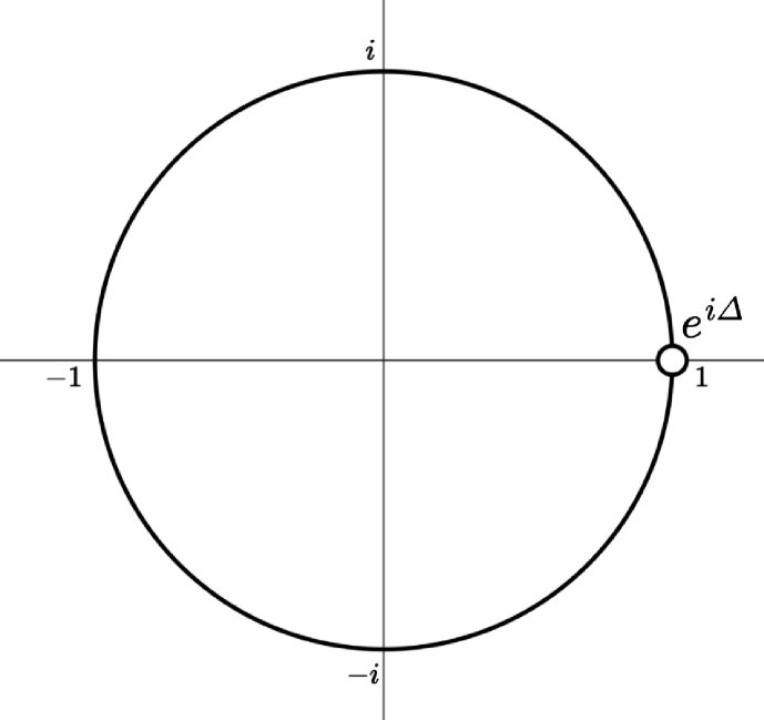
(a) Eigenvalue of $U$

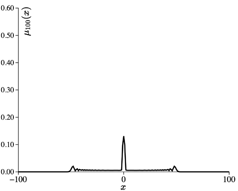
(b) Probability distribution

Figure 1: Example of Proposition 3.2 with parameters $\displaystyle\Delta_{o}=\Delta=0,\ \theta_{o}=\frac{8}{12},\ \theta=-\frac{8}{12}\pi$. (a) illustrates the eigenvalue, and (b) shows the probability distribution at time $100$ with initial state $\Psi_{0}(0)=[\frac{1}{\sqrt{3}},\frac{i}{\sqrt{3}},\frac{1}{\sqrt{3}}]^{t}$ and $\Psi_{0}(x)=\mathbf{0}$ for $x\neq 0$.

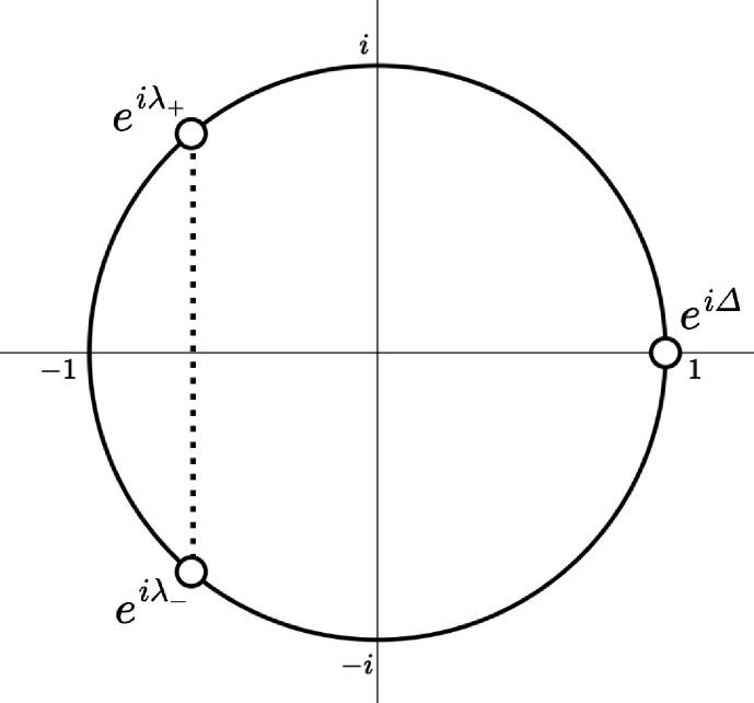
(a) Eigenvalues of $U$

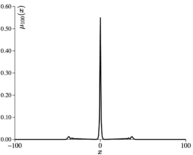
(b) Probability distribution

Figure 2: Example of Proposition 3.2 with parameters $\displaystyle\Delta_{o}=\Delta=0,\ \theta_{o}=\frac{8}{12}\pi,\ \theta=-\frac{9}{12}\pi$. (a) illustrates the eigenvalues, and (b) shows the probability distribution at time $100$ with initial state $\Psi_{0}(0)=[\frac{1}{\sqrt{3}},\frac{i}{\sqrt{3}},\frac{1}{\sqrt{3}}]^{t}$ and $\Psi_{0}(x)=\mathbf{0}$ for $x\neq 0$

3.3 Two-phase model

Here, we consider the two-phase model, where $C_{o}=C_{p}$. In the case which $\lambda$ does not satisfy Assumption 2.2, i.e, $e^{i\lambda}=e^{i\Delta_{m}},e^{i\Delta_{p}}$, Lemma 3.1 shows $e^{i\Delta_{m}},e^{i\Delta_{p}}\in\sigma_{p}(U)$. Next, under the Assumption 2.2, i.e., $e^{i\lambda}\neq e^{i\Delta_{m}},e^{i\Delta_{p}}$, Theorem 2.3 shows that $e^{i\lambda}\in\sigma_{p}(U)$ if and only if followings hold:

$$1. \ e^{i\lambda}=\frac{(c_{p}-c_{m})\pm i\sqrt{2(1-c_{m})(1-c_{p})(1-\cos(\Delta_{m}-\Delta_{p}))}}{\left((1-c_{m})e^{-i\Delta_{p}}-(1-c_{p})e^{-i\Delta_{m}}\right)},$$

$$2. \ \sin(\lambda-\Delta_{p})\sin(\lambda-\Delta_{m})<0,$$

$$3. \ \cos(\lambda-\Delta_{m})>c_{m}.$$

Note that $\cos(\lambda-\Delta_{m})>c_{m}$ is equivalent to $\cos(\lambda-\Delta_{p})>c_{p}$ in this model.

Proposition 3.3.

When $\Delta_{m}=\Delta_{p}=\Delta$

$$\sigma_{p}(U)=\left\{e^{i\Delta}\right\}.$$

Proposition 3.4.

When $c_{m}=c_{p}=c$ and $\Delta_{m}\neq\Delta_{p}$, let

$$condition\ 1: \ \frac{\sin(\Delta_{m}-\Delta_{p})}{\sqrt{2(1-\cos(\Delta_{m}-\Delta_{p}))}}>-c,$$

$$condition\ 2: \frac{\sin(\Delta_{m}-\Delta_{p})}{\sqrt{2(1-\cos(\Delta_{m}-\Delta_{p}))}}<c.$$

Then

$$\sigma_{p}(U)=\begin{cases}\left\{e^{i\Delta_{m}},e^{i\Delta_{p}}\right\},&if\ neither\ condition\ 1\ nor\ condition\ 2\ holds,\\ \left\{e^{i\Delta_{m}},e^{i\Delta_{p}},e^{i\lambda}\right\},&if\ condition\ 1\ holds\ and\ condition\ 2\ does\ not,\\ \left\{e^{i\Delta_{m}},e^{i\Delta_{p}},-e^{i\lambda}\right\},&if\ condition\ 2\ holds\ and\ condition\ 1\ does\ not,\\ \left\{e^{i\Delta_{m}},e^{i\Delta_{p}},e^{i\lambda},-e^{i\lambda}\right\},&if\ both\ conditions\ 1\ and\ 2\ hold,\end{cases}$$

where

$$e^{i\lambda}=\frac{i\left(e^{i\Delta_{p}}-e^{i\Delta_{m}}\right)}{\sqrt{2(1-\cos(\Delta_{m}-\Delta_{p}))}}.$$

The examples of proposition 3.4 are shown in Figures 3, 4.

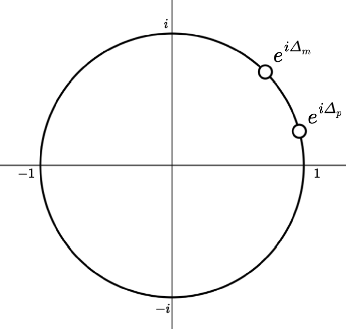
(a) Eigenvalues of $U$

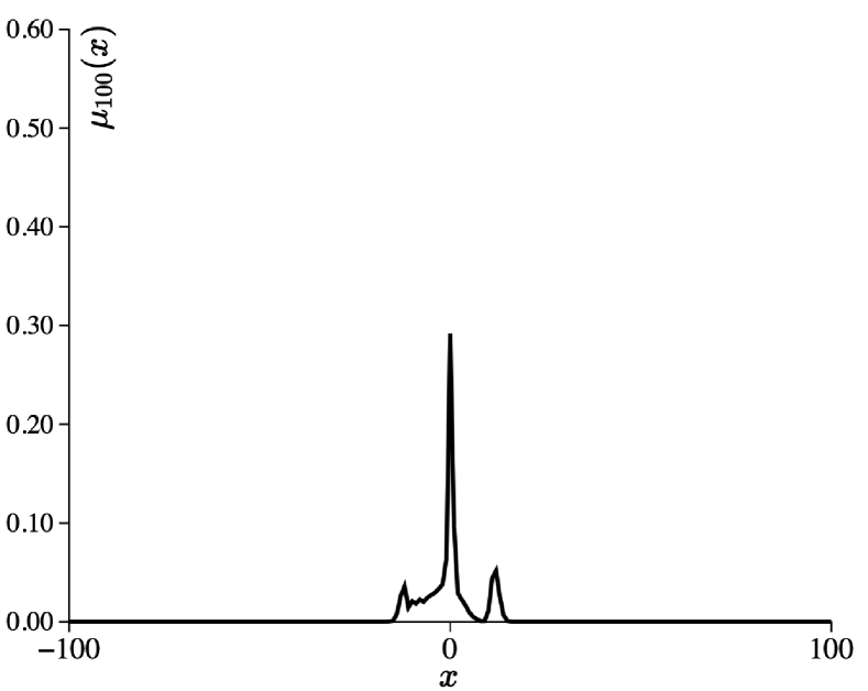
(b) Probability distribution

Figure 3: Example of Proposition 3.4 with parameters $\displaystyle\Delta_{m}=\frac{3}{12}\pi,\ \Delta_{p}=\frac{1}{12}\pi,\ \theta=\frac{11}{12}\pi$. (a) illustrates the eigenvalues, and (b) shows the probability distribution at time $100$ with initial state $\Psi_{0}(0)=[\frac{1}{\sqrt{3}},\frac{i}{\sqrt{3}},\frac{1}{\sqrt{3}}]^{t}$ and $\Psi_{0}(x)=\mathbf{0}$ for $x\neq 0$

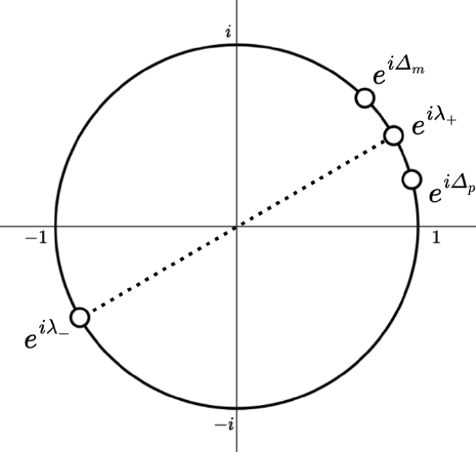
(a) Eigenvalues of $U$

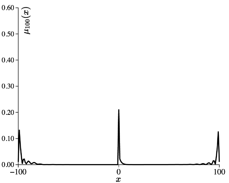
(b) Probability distribution

Figure 4: Example of Proposition 3.4 with parameters $\displaystyle\Delta_{m}=\frac{3}{12}\pi,\ \Delta_{p}=\frac{1}{12}\pi,\ \theta=\frac{1}{12}\pi$. (a) illustrates the eigenvalues, and (b) shows the probability distribution at time $100$ with initial state $\Psi_{0}(0)=[\frac{1}{\sqrt{3}},\frac{i}{\sqrt{3}},\frac{1}{\sqrt{3}}]^{t}$ and $\Psi_{0}(x)=\mathbf{0}$ for $x\neq 0$

4 Summary

In this paper, we analyzed eigenvalues of two-phase three-state generalized Grover walks with one defect in one dimension. In Section 2, we successfully derived Theorem 2.3 via transfer matrices, which is the necessary and sufficient condition for the eigenvalue problem for $n$-state QWs with $n-2$ self-loops under the Assumption 2.2. Next, we focused on the eigenvalue problem for three-state generalized Grover walks in Section 3. Lemma 3.1 revealed that $e^{i\Delta_{\pm\infty}}$ are eigenvalues of $U$, which also indicates that these models always exhibit localization. Subsequently, by applying Theorem 2.3, we got the necessary and sufficient condition for the eigenvalue problem and successfully calculated concrete eigenvalues for one-defect model in Propositions 3.2, and two-phase models in Propositions 3.3 and 3.4.

References

- [1] Andris Ambainis et al. “One-dimensional quantum walks” In Proceedings of the thirty-third annual ACM symposium on Theory of computing, STOC ’01 Hersonissos, Greece: Association for Computing Machinery, 2001, pp. 37–49
- [2] Norio Konno “Quantum Random Walks in One Dimension” In Quantum Inf. Process. 1.5, 2002, pp. 345–354
- [3] Norio Inui, Norio Konno and Etsuo Segawa “One-dimensional three-state quantum walk” In Phys. Rev. E Stat. Nonlin. Soft Matter Phys. 72.5 Pt 2, 2005, pp. 056112
- [4] Caishi Wang, Wenling Wang and d Xiangying Lu “Limit Theorem for a Time-Inhomogeneous Three-State Quantum Walk on the Line” In J. Comput. Theor. Nanosci. 12.12, 2015, pp. 5164–5170
- [5] Takako Endo, Takashi Komatsu, Norio Konno and Tomoyuki Terada “Stationary measure for three-state quantum walk” In Quantum Inf. Comput. 19.11&12 Rinton Press, 2019, pp. 901–912
- [6] Jishnu Rajendran and Colin Benjamin “Playing a true Parrondo’s game with a three-state coin on a quantum walk” In EPL 122.4 IOP Publishing, 2018, pp. 40004
- [7] Caishi Wang, Xiangying Lu and Wenling Wang “The stationary measure of a space-inhomogeneous three-state quantum walk on the line” In Quantum Inf. Process. 14.3 Springer ScienceBusiness Media LLC, 2015, pp. 867–880
- [8] P R N Falcão et al. “Universal dynamical scaling laws in three-state quantum walks”, 2021 arXiv:2108.10275 [quant-ph]
- [9] Amit Saha, Sudhindu Bikash Mandal, Debasri Saha and Amlan Chakrabarti “One-Dimensional Lazy Quantum Walk in Ternary System” In IEEE Trans. Quant. Eng. 2, 2021, pp. 1–12
- [10] Norio Inui and Norio Konno “Localization of multi-state quantum walk in one dimension” In Phys. A: Stat. Mech. Appl. 353, 2005, pp. 133–144
- [11] M Štefaňák, I Bezděková and I Jex “Limit distributions of three-state quantum walks: The role of coin eigenstates” In Phys. Rev. A 90.1 American Physical Society, 2014, pp. 012342
- [12] Stefan Falkner and Stefan Boettcher “Weak limit of the three-state quantum walk on the line” In Phys. Rev. A 90.1 American Physical Society, 2014, pp. 012307
- [13] Dan Li, Michael Mc Gettrick, Wei-Wei Zhang and Ke-Jia Zhang “One-dimensional lazy quantum walks and occupancy rate” In Chin. Phys. B 24.5, 2015, pp. 050305
- [14] Takuya Machida “Limit theorems of a 3-state quantum walk and its application for discrete uniform measures” In Quantum Inf. Comput., 2015, pp. 406–418
- [15] Yong-Zhen Xu, Gong-De Guo and Song Lin “One-Dimensional Three-State Quantum Walk with Single-Point Phase Defects” In Int. J. Theor. Phys. 55.9, 2016, pp. 4060–4074
- [16] Chusei Kiumi “A new type of quantum walks based on decomposing quantum states” In Quantum Inf. Comput. 21.7&8 Rinton Press, 2021, pp. 541–556
- [17] Lov K Grover “A fast quantum mechanical algorithm for database search” In Proceedings of the twenty-eighth annual ACM symposium on Theory of Computing, STOC ’96 Philadelphia, Pennsylvania, USA: Association for Computing Machinery, 1996, pp. 212–219
- [18] Norio Konno “Localization of an inhomogeneous discrete-time quantum walk on the line” In Quantum Inf. Process. 9.3, 2010, pp. 405–418
- [19] M J Cantero, F A Grünbaum, L Moral and L Velázquez “The CGMV method for quantum walks” In Quantum Inf. Process. 11.5 Springer ScienceBusiness Media LLC, 2012, pp. 1149–1192
- [20] Takako Endo, Norio Konno and Hideaki Obuse “Relation between two-phase quantum walks and the topological invariant” In Yokohama Math. J. 64, 2020
- [21] Takako Endo, Norio Konno, Etsuo Segawa and Masato Takei “A one-dimensional Hadamard walk with one defect” In Yokohama Math. J. 60, 2014, pp. 49–90
- [22] Shimpei Endo et al. “Limit theorems of a two-phase quantum walk with one defect” In Quantum Inf. Comput. 15.15&16 Rinton Press, 2015, pp. 1373–1396
- [23] Antoni Wójcik et al. “Trapping a particle of a quantum walk on the line” In Phys. Rev. A 85.1 American Physical Society, 2012, pp. 012329
- [24] Shimpei Endo, Takako Endo, Takashi Komatsu and Norio Konno “Eigenvalues of Two-State Quantum Walks Induced by the Hadamard Walk” In Entropy 22.1, 2020
- [25] Chusei Kiumi and Kei Saito “Eigenvalues of two-phase quantum walks with one defect in one dimension” In Quantum Inf. Process. 20.5 Springer ScienceBusiness Media LLC, 2021
- [26] Andris Ambainis, Julia Kempe and Alexander Rivosh “Coins make quantum walks faster” In Proceedings of the sixteenth annual ACM-SIAM symposium on Discrete algorithms, SODA ’05 Vancouver, British Columbia: Society for IndustrialApplied Mathematics, 2005, pp. 1099–1108
- [27] Andrew M Childs and Jeffrey Goldstone “Spatial search by quantum walk” In Phys. Rev. A 70.2 American Physical Society, 2004, pp. 022314
- [28] Neil Shenvi, Julia Kempe and K Birgitta Whaley “Quantum random-walk search algorithm” In Phys. Rev. A 67.5 American Physical Society, 2003, pp. 052307
- [29] Takuya Kitagawa, Mark S Rudner, Erez Berg and Eugene Demler “Exploring topological phases with quantum walks” In Phys. Rev. A 82.3 American Physical Society, 2010, pp. 033429
- [30] Etsuo Segawa and Akito Suzuki “Generator of an abstract quantum walk” In Quantum Studies: Mathematics and Foundations 3.1, 2016, pp. 11–30
- [31] Chusei Kiumi and Kei Saito “Strongly trapped space-inhomogeneous quantum walks in one dimension”, 2021 arXiv:2105.10962 [math-ph]
- [32] Hikar Kawai, Takashi Komatsu and Noriko Konno “Stationary measures of three-state quantum walks on the one-dimensional lattice” In Yokohama Math. J. 63, 2017, pp. 59–74
- [33] Hikari Kawai, Takashi Komatsu and Norio Konno “Stationary measure for two-state space-inhomogeneous quantum walk in one dimension” In Yokohama Math. J. 64, 2018, pp. 111–130
- [34] B Danacı, G Karpat, İ Yalçınkaya and A L Subaşı “Non-Markovianity and bound states in quantum walks with a phase impurity” In J. Phys. A: Math. Theor. 52.22 IOP Publishing, 2019, pp. 225302