Enhanced sensitivity of an all-dielectric refractive index sensor with optical bound state in the continuum

Abstract

The sensitivity of a refractive index sensor based on an optical bound state in the continuum is considered. Applying Zel’dovich perturbation theory we derived an analytic expression for bulk sensitivity of an all-dielectic sensor utilizing symmetry protected in-$\Gamma$ optical bound states in a dielectric grating. The upper sensitivity limit is obtained. A recipe is proposed for obtaining the upper sensitivity limit by optimizing the design of the grating. The results are confirmed through direct numerical simulations.

Introduction

Recently, we have witnessed a surge of interest to bound states in the continuum (BICs) Hsu et al. (2016); Koshelev et al. (2019a); Sadreev (2021) that have revolutionized nanophotonics by paving a way to high throughput optical sensing devices with enhanced light-matter interaction at the nanoscale Molina et al. (2012); Romano et al. (2018a); Bulgakov and Sadreev (2008); Penzo et al. (2017); Zhen et al. (2014); Mocella and Romano (2015); Koshelev et al. (2019b); Zito et al. (2019). The most remarkable feature of BICs is the occurrence of high-quality Fano resonances in the transmittance spectrum Shipman and Venakides (2005); Sadreev et al. (2006); Blanchard et al. (2016); Bulgakov and Maksimov (2018a). The Fano resonances emerge when the system’s symmetry is broken, so the otherwise localized BIC mode can couple with impinging light Koshelev et al. (2018); Maksimov et al. (2020). The spectral position of these extremely narrow Fano resonances is affected by the refractive index of the surrounding medium allowing to design optical sensors with an excellent figure of merit (FOM) Liu et al. (2017); Romano et al. (2018b, c); Yesilkoy et al. (2019); Mukherjee et al. (2019); Vyas and Hegde (2020) as the narrow Fano feature can be easily resolved in the spectral measurements. Despite the unsurpassed FOM, the major drawback of the dielectric sensors in comparison against the plasmonic ones is a noticeably (approximately five times) less sensitivity Bosio et al. (2019). Nowadays, comparative analysis of dielectric sensors performance is already available in the existing literature Pitruzzello and Krauss (2018); Wang et al. (2021). Yet, to the best of our knowledge, there is no exhaustive theory providing a clear optimization procedure that would lead to the maximal sensitivity of a BIC sensor. In our previous paper Maksimov et al. (2020) we argued that the maximal sensitivity of a BIC sensor is given by $S_{\mathrm{max}}=\lambda_{\mathrm{BIC}}/n_{c}$, where $\lambda_{\mathrm{BIC}}$ is the vacuum wavelength of the BIC, and $n_{c}$ is the the cladding fluid refractive index, i.e. the physical quantity whose variation is measured by the sensor. In this paper we provide a rout for achieving the above limit by considering an optical BICs whose spectral position approach the frequency cut-offs of the first order diffraction channels. An analytic expression for a BIC vacuum wavelength shift is derived by applying the Zel’dovich perturbation theory Zel’dovich (1961). The primary advantage of the Zel’dovich approach is that it can be applied to optical delocalized eigenmodesLai et al. (1990) to have already been proved useful in theory of plasmonic sensors Zalyubovskiy et al. (2012). The onset of diffraction usually has a negative impact on high-Q resonances, particularly on BICs which are typically destroyed by the radiation losses Sadrieva et al. (2017). However, in the situation when the first order diffraction cut-off frequency is not yet exceeded the evanescent field are demonstrated to provide the largest overlap with the cladding fluid leading to enhanced sensitivity Romano et al. (2019).

The system

One of the most important platforms for implementing optical BICs is subwavelength dielectric gratings Marinica et al. (2008); Sadrieva et al. (2017); Monticone and Alù (2017); Bulgakov et al. (2018); Bulgakov and Maksimov (2018b); Lee and Magnusson (2019); Bykov et al. (2019); Gao et al. (2019); Hemmati and Magnusson (2019) which have been extensively studied for sensing applications with both dielectric Maksimov et al. (2020); Zhang et al. (2021); Finco et al. (2021); Park and Park (2021); Mesli et al. (2021) and plasmonic structures Jia et al. (2021). The system under consideration is a subwavelength dielectric grating of period $h=300{\rm nm}$ made of ${\rm TiO}_{2}$. In our numerical simulations we use $n_{g}=2.485$ as the refractive index of the grating while the material losses are ignored so the absorption coefficient is set to zero. The ${\rm TiO}_{2}$ grating is placed on top of a glass substrate with refractive index $n_{s}=1.5$ as shown in Fig. 1 (a). The geometric parameters of the grating are specified in the caption to Fig. 1.

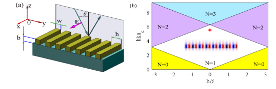
Figure 1: BIC in dielectric grating. (a) ${\rm TiO}_{2}$ dielectric grating on a glass substrate, $h=300nm$, $b=0.5h$, $w=0.5h$, $n_{g}=2.485$, and $n_{s}=1.5$. The magenta arrow is the electric vector of an incident $s$-wave; (b) Number of scattering channels allowed for diffraction. The red star indicates the position of a symmetry protected BIC with $k_{{\rm BIC}}=3.262$, $n_{c}=1.7$. The BIC mode profile is depicted below its spectral position in procedure defined units with red areas corresponding to positive $E_{x}$ whereas in the blue areas $E_{x}$ is negative.

Propagation of TE modes is controlled by the Helmholtz equation

$$\nabla^{2}E_{x}(y,z)+k^{2}\epsilon(y,z)E_{x}(y,z)=0,$$ (1)

where $E_{x}$ is the $x$-component of the electric field, $\epsilon=f(y,z)$ — the coordinate dependant dielectric function, $\nabla^{2}$ — the 2D Laplacian operator, and $k=\omega/c$ is the vacuum wave-number. The spectrum of far-field diffraction channels available for scattering is given by

$$n_{c}k^{2}=\left(\beta+\frac{2\pi m}{h}\right)^{2}+k_{z}^{2},\ m=-\infty,\ldots,-1,0,1,\ldots,\infty,$$ (2)

where $k_{z}$ is the $z$ component of the outgoing wave vector, $\beta$ is the propagation constant with respect to the $y$-axis, and $n_{c}$ is the refractive index of the cladding fluid. All simulation results referenced throughout the paper have been obtained with application of FDTD Lumerical photonics simulation software solution.

Following our previous work Maksimov et al. (2020) we consider a symmetry protected in-$\Gamma$ BIC which does not radiate to the far field because it is symmetrically mismatched with the zeroth-order diffraction channel at strict normal incidence. In engineering a symmetry protected BIC it is of key importance to ensure that the higher diffraction orders are not allowed at the BIC wavelength. Once diffraction is allowed either in the substrate or in the superstrate (cladding fluid) the BIC is destroyed being transformed into a leaky mode radiating into the diffraction channels Sadrieva et al. (2017). The onset of diffraction is typically detected by occurrence of Wood-Rayleigh anomaly in the scattering spectra Wood (1902); Rayleigh (1907). The positions of Wood’s anomalies are given by the following equations

$$n_{c}k=|\beta|,$$

$$n_{c}k=\beta+\frac{2\pi m}{h}\ \mathrm{if}\ m>0,$$

$$n_{c}k=-\beta-\frac{2\pi m}{h}\ \mathrm{if}\ m<0.$$ (3)

In Fig. 1 (b) we demonstrate the number of diffraction channels $N$ allowed in the cladding depending on the spectral parameters of the incident wave, namely its vacuum wavelength, $k$ and the propagation constant in the $y$-direction, $\beta$. Each colored domain in Fig. 1 (b) corresponds to the specified value of $N$. Wood’s anomalies occur when the boundaries between the domains with $N>1$ are crossed under variation of the spectral parameters of the incident wave. The symmetry protected BICs can be found in the domain of specular reflection $N=1$. The spectral position of such a BIC with $n_{c}=1.7$ is shown in 1 (b) by a red plus sign. The BIC mode profile is set in the middle. It is important for our future purpose to point out that the BIC mode profile has the following asymptotic far-field expression

$$E_{x}\propto e^{-\varkappa z}\sin\left(\frac{2\pi y}{h}\right),$$ (4)

where

$$\varkappa=\sqrt{\left(\frac{2\pi}{h}\right)^{2}-\epsilon^{\scriptscriptstyle{(0)}}_{\infty}k^{2}}$$ (5)

with $\epsilon^{\scriptscriptstyle{(0)}}_{\infty}=n_{c}^{2}$ and $y=0$ corresponding to the geometric center of the unit cell. Notice that in Equation (4) we only retained the contribution of the first order evanescent diffraction channels, since the higher order channels decay much faster with the increase of $z$.

Perturbation theory

The Zel’dovich Zel’dovich (1961) perturbation approach is introduced by writing a series expansion in the increment of the dielectric function $\Delta\epsilon$

$$\epsilon=\epsilon^{\scriptscriptstyle{(0)}}+\Delta\epsilon,$$

$$k=k^{\scriptscriptstyle{(0)}}+\Delta k,$$

$$E_{x}=E_{x}^{\scriptscriptstyle{(0)}}+E_{x}^{\scriptscriptstyle{(1)}}.$$ (6)

By definition the function $\epsilon^{\scriptscriptstyle{(0)}}$ is the total coordinate dependent dielectric function with the reference value of the cladding fluid refractive index, whereas $\Delta\epsilon$ is the increment of the dielectric constant of the cladding fluid. Substituting the above into Equation (1) we have up to the first perturbation order

$$\nabla^{2}E_{x}^{\scriptscriptstyle{(0)}}+\epsilon^{\scriptscriptstyle{(0)}}(k^{\scriptscriptstyle{(0)}})^{2}E_{x}^{\scriptscriptstyle{(0)}}=0,$$ (7)

$$\nabla^{2}E_{x}^{\scriptscriptstyle{(1)}}+\epsilon^{\scriptscriptstyle{(0)}}(k^{\scriptscriptstyle{(0)}})^{2}E_{x}^{\scriptscriptstyle{(1)}}=-\Delta\epsilon(k^{\scriptscriptstyle{(0)}})^{2}E_{x}^{\scriptscriptstyle{(0)}}-2\epsilon^{\scriptscriptstyle{(0)}}\Delta kk^{\scriptscriptstyle{(0)}}E_{x}^{\scriptscriptstyle{(0)}}.$$ (8)

Following Zel’dovich we multiply Equation (8) by $E_{x}^{\scriptscriptstyle{(0)}}$ and integrate within the limits specified below

$$\int\limits_{-{h}/{2}}^{{h}/{2}}dy\int\limits_{-d}^{d}dzE_{x}^{\scriptscriptstyle{(0)}}[\nabla^{2}E_{x}^{\scriptscriptstyle{(1)}}+\epsilon^{\scriptscriptstyle{(0)}}(k^{\scriptscriptstyle{(0)}})^{2}E_{x}^{\scriptscriptstyle{(1)}}]=-\int\limits_{-{h}/{2}}^{{h}/{2}}dy\int\limits_{-d}^{d}dz[\Delta\epsilon(k^{\scriptscriptstyle{(0)}})^{2}+2\epsilon^{\scriptscriptstyle{(0)}}\Delta kk^{\scriptscriptstyle{(0)}}](E_{x}^{\scriptscriptstyle{(0)}})^{2},$$ (9)

where $d>b$ is an arbitrary distance from the grating. By applying Green’s theorem together with Equation (7) one rewrites the L.H.P. of Equation (9) in the following manner

$$\int\limits_{-{h}/{2}}^{{h}/{2}}dy\int\limits_{-d}^{d}dzE_{x}^{\scriptscriptstyle{(0)}}[\nabla^{2}E_{x}^{\scriptscriptstyle{(1)}}+\epsilon^{\scriptscriptstyle{(0)}}(k^{\scriptscriptstyle{(0)}})^{2}E_{x}^{\scriptscriptstyle{(1)}}]=\int\limits_{\ell}d\ell\left(E_{x}^{\scriptscriptstyle{(0)}}\frac{\partial E_{x}^{\scriptscriptstyle{(1)}}}{\partial n}-E_{x}^{\scriptscriptstyle{(1)}}\frac{\partial E_{x}^{\scriptscriptstyle{(0)}}}{\partial n}\right),$$ (10)

where $\ell$ is a path encircling the integration domain of the L.H.P. in the clockwise direction. The integrals along the lines $y=-h/2$ and $y=h/2$ cancel each other due to periodicity while the integral along $z=-d$ can be neglected as we assume that the BIC field decays faster in the substrate because of a lesser refractive index. This leads us to

$$\int\limits_{-{h}/{2}}^{{h}/{2}}dy\int\limits_{-d}^{d}dzE_{x}^{\scriptscriptstyle{(0)}}[\nabla^{2}E_{x}^{\scriptscriptstyle{(1)}}+\epsilon^{\scriptscriptstyle{(0)}}(k^{\scriptscriptstyle{(0)}})^{2}E_{x}^{\scriptscriptstyle{(1)}}]=\int\limits_{-h/2}^{h/2}dy\left(E_{x}^{\scriptscriptstyle{(0)}}(y,d)\frac{\partial E_{x}^{\scriptscriptstyle{(1)}}(y,d)}{\partial z}-E_{x}^{\scriptscriptstyle{(1)}}(y,d)\frac{\partial E_{x}^{\scriptscriptstyle{(0)}}(y,d)}{\partial z}\right).$$ (11)

Equating the R.H.P. of Equation (11) to that of Equation (9) and inserting the following asymptotic expressions

$$\frac{\partial E_{x}^{\scriptscriptstyle{(0)}}}{\partial z}=-\varkappa^{\scriptscriptstyle{(0)}}E_{x}^{\scriptscriptstyle{(0)}},$$

$$\frac{\partial E_{x}^{\scriptscriptstyle{(1)}}}{\partial z}=\frac{1}{2\varkappa^{\scriptscriptstyle{(0)}}}[\Delta\epsilon(k^{\scriptscriptstyle{(0)}})^{2}+2\epsilon^{\scriptscriptstyle{(0)}}_{\infty}k^{\scriptscriptstyle{(0)}}\Delta k]E_{x}^{\scriptscriptstyle{(0)}}-\varkappa^{\scriptscriptstyle{(0)}}E_{x}^{\scriptscriptstyle{(1)}},$$ (12)

one has

$$\frac{\Delta k}{\Delta\epsilon}=-\frac{k^{\scriptscriptstyle{(0)}}}{2}I,$$ (13)

where

$$I=\frac{\displaystyle\int\limits_{S_{\rm c}}dS\left(E_{x}^{\scriptscriptstyle{(0)}}\right)^{2}+\frac{1}{2\varkappa^{\scriptscriptstyle{(0)}}}\displaystyle\int\limits_{-h/2}^{h/2}dy\left[E_{x}^{\scriptscriptstyle{(0)}}(y,d)\right]^{2}}{\displaystyle\int\limits_{S_{\rm tot}}dS\epsilon^{\scriptscriptstyle{(0)}}\left(E_{x}^{\scriptscriptstyle{(0)}}\right)^{2}+\frac{\epsilon^{\scriptscriptstyle{(0)}}_{\infty}}{2\varkappa^{\scriptscriptstyle{(0)}}}\int\limits_{-h/2}^{h/2}dy\left[E_{x}^{\scriptscriptstyle{(0)}}(y,d)\right]^{2}}.$$ (14)

Thus, for the differential sensitivity $S=\Delta\lambda_{\scriptscriptstyle{\mathrm{BIC}}}/\Delta n_{c}$ we have

$$S=\lambda n_{c}I.$$ (15)

On approach to the cut-off of the first order diffraction channels $\varkappa\rightarrow 0$ we have

$$S=\frac{\lambda_{\scriptscriptstyle{\mathrm{BIC}}}}{n_{c}}$$ (16)

which coincides with the upper sensitivity limit predicted in Maksimov et al. (2020). Before proceeding to numerical validation of the newfound results some comments are due on the choice of $d$. It is obvious that $d$ should be taken large enough to guarantee that the far-field asymptotic behaviour be given by Equation (4). In the domain of specular reflection at the normal incidence the evanescent fields of the second order diffraction channels decay faster than $e^{-2\pi z/h}$. Therefore, for a practical choice it is sufficient to take $d>\lambda_{\scriptscriptstyle{\rm BIC}}$. At the save time, from the computation viewpoint the choice of $d$ determines the size of the computational domain. Technically, $d$ is the distance at which the PML absorbers are placed to set-up reflectionless boundary conditions. Thus, application of Equations (14, 15) allows us to predict the sensitivity of BICs with the evanescent fields extended beyond the computational domain.

Numerical validation

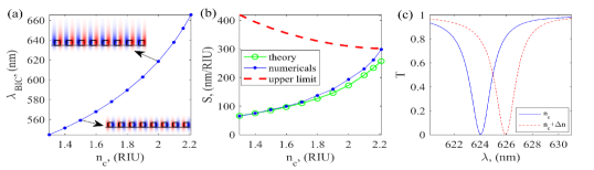
Figure 2: Fano resonance shift and differential sensitivity. (a) The vacuum wavelength of the symmetry protected BIC as a function of the cladding fluid refractive index. (b) Differential sensitivity obtained from Equation (15) — green circles, and through the shift of the Fano resonance — blue dots at $\theta=2(\mathrm{deg})$. (c) Shift of the Fano resonance obtained at $\theta=2(\mathrm{deg})$, $n_{c}=2.0$ with $\Delta n=0.01$.

In Fig. 2 (a) we plotted the vacuum wavelength of the symmetry protected BIC at different values of $n_{c}$. One can see from Fig. 2 (a) that $\lambda_{\mathrm{\scriptscriptstyle{BIC}}}$ decreases with the increase of $n_{c}$ especially at larger values of $n_{c}$. In Fig. 2 (b) we plotted the values of differential sensitivity obtained by two different methods. The "theoretical" result is obtained by directly applying Equation (15) meanwhile the "numerical" values are obtained finding the shift of a BIC-induced Fano resonance under illumination by a plane wave at the incidence angle $\theta=2(\mathrm{deg})$. To keep the approach consistent while changing $n_{c}$, the incidence angle $\theta$ is defined in reference to the wave vectors in the outer space (air), so the incident angle within the cladding fluid $\theta_{c}$ is found through the formula

$$n_{c}\sin(\theta_{c})=\sin(\theta).$$ (17)

The typical picture of the shift in the resonance position is shown in Fig. 2 (c). In Fig. 2 (b) we also plotted the maximal value of the sensitivity according to Equation (16). One can see from Fig. 2 (b) that with the increase of $n_{c}$ the sensitivity approach the upper limit given by Equation (16). Notice that at larger $n_{c}$ the numerically observed sensitivity deviates from the theoretical expressions (14, 15). This is because the first order frequency cut-offs are lower at $\theta\neq 0$ according to Equation (The system), see also Fig. 2 (b). In our case the onset of diffraction at $n_{c}=2.21$ destroys the high-Q resonance with the chosen angle of incidence $\theta=2\mathrm{(deg)}$ although the BIC proper is not yet destroyed. Finally, notice that the observed sensitivity enhancement can be easily understood from Fig. 2 (a) which is complemented with subplots of two BIC mode profiles. One can see that at larger $n_{c}$ the BIC fields are further extended into the upper half-space providing a better overlap with the cladding fluid.

Conclusion

In this paper we have demonstrated an approach allowing to achieve the upper sensitivity limit for an all-dielectric sensor based on an optical bound state in the continuum (BIC). The analytic expressions for computing the bulk sensitivity from the BIC vacuum wavelength and mode profile have been derived as Equations (14, 15). The most remarkable feature of the obtained expressions is that the maximal sensitivity is independent of the material and geometric parameters of the grating allowing for freedom in choosing of the constituent dielectric. All that is necessary for achieving the maximal sensitivity is to vary the geometric parameters for the BIC eigenfrequency approaching the cut-offs of the first order diffraction channels. The BICs are topologically protected objects Zhen et al. (2014); Bulgakov and Maksimov (2017a, b) and therefore are bit destroyed under variation of geometric parameters complying with the structure point group symmetry as far as the BIC eigenfrequency remains in the spectral domain of the specular reflection Bulgakov et al. (2018). In the regime of maximal sensitivity the vacuum wavelength of the in-$\Gamma$ BIC is always given by

$$\lambda_{\scriptscriptstyle{\mathrm{BIC}}}=n_{c}h,$$ (18)

while the maximal sensitivity is simply $S_{\scriptscriptstyle{\mathrm{max}}}=\lambda_{\scriptscriptstyle{\mathrm{BIC}}}/n_{c}$. Notice that due to the scaling invariance of Maxwell’s equations, $\lambda_{\scriptscriptstyle{\mathrm{BIC}}}$ can be tuned to any desired wavelength by isometric transformation of the grating.

In the numerical example proposed the maximal sensitivity has been achieved with a relatively large value of the cladding fluid refractive index $n_{c}=2.21$. This, of course, out of the range required in practical applications which are stuck around the refractive index of water. Importantly, achieving the maximal sensitivity requires the refractive index of the cladding larger than that of substrate. If the situation is the opposite, the first order diffraction channels will first open in the substrate Sadrieva et al. (2017) destroying the BIC before the maximal overlap with the cladding has been achieved. There are two possible solutions to this problem. The first is, obviously, applying a low index substrate Schubert et al. (2007). The second is using a substrate of a properly chosen Bragg reflector Bikbaev et al. (2021) which would isolate the lower half-space by a photonic band gap for the outgoing waves of the first order of diffraction. This problem will be addressed in the future studies.

Author contributions statement

D.N.M. and A.A.B conceived the idea presented. D.N.M. derived the analytic results. V.S.G. ran numerical simulations. S.P.P. supervised the project. All authors have equally contributed to writing the paper.

Additional information

Competing interests: The authors declare no competing interests.

Data availability: The data that support the findings of this study are available from the corresponding author, D.N.M., upon reasonable request.

References

- Hsu et al. (2016) Chia Wei Hsu, Bo Zhen, A. Douglas Stone, John D. Joannopoulos, and Marin Soljačić, “Bound states in the continuum,” Nature Reviews Materials 1, 16048 (2016).
- Koshelev et al. (2019a) Kirill Koshelev, Gael Favraud, Andrey Bogdanov, Yuri Kivshar, and Andrea Fratalocchi, “Nonradiating photonics with resonant dielectric nanostructures,” Nanophotonics 8, 725–745 (2019a).
- Sadreev (2021) Almas F Sadreev, “Interference traps waves in open system: Bound states in the continuum,” Reports on Progress in Physics (2021).
- Molina et al. (2012) Mario I Molina, Andrey E Miroshnichenko, and Yuri S Kivshar, “Surface bound states in the continuum,” Physical review letters 108, 070401 (2012).
- Romano et al. (2018a) Silvia Romano, Gianluigi Zito, Stefano Managò, Giuseppe Calafiore, Erika Penzo, Stefano Cabrini, Anna Chiara De Luca, and Vito Mocella, “Surface-enhanced raman and fluorescence spectroscopy with an all-dielectric metasurface,” The Journal of Physical Chemistry C 122, 19738–19745 (2018a).
- Bulgakov and Sadreev (2008) Evgeny N Bulgakov and Almas F Sadreev, “Bound states in the continuum in photonic waveguides inspired by defects,” Physical Review B 78, 075105 (2008).
- Penzo et al. (2017) Erika Penzo, Silvia Romano, Yu Wang, Scott Dhuey, Luca Dal Negro, Vito Mocella, and Stefano Cabrini, “Patterning of electrically tunable light-emitting photonic structures demonstrating bound states in the continuum,” J. Vac. Sc.& Tech. B 35, 06G401 (2017).
- Zhen et al. (2014) Bo Zhen, Chia Wei Hsu, Ling Lu, A. Douglas Stone, and Marin Soljačić, “Topological nature of optical bound states in the continuum,” Physical Review Letters 113, 257401 (2014).
- Mocella and Romano (2015) V. Mocella and S. Romano, “Giant field enhancement in photonic resonant lattices,” Physical Review B 92, 155117 (2015).
- Koshelev et al. (2019b) Kirill Koshelev, Andrey Bogdanov, and Yuri Kivshar, “Meta-optics and bound states in the continuum,” Science Bulletin 64, 836–842 (2019b).
- Zito et al. (2019) Gianluigi Zito, Silvia Romano, Stefano Cabrini, Giuseppe Calafiore, Anna Chiara De Luca, Erika Penzo, and Vito Mocella, “Observation of spin-polarized directive coupling of light at bound states in the continuum,” Optica 6, 1305–1312 (2019).
- Shipman and Venakides (2005) Stephen P Shipman and Stephanos Venakides, “Resonant transmission near nonrobust periodic slab modes,” Physical Review E 71, 026611 (2005).
- Sadreev et al. (2006) Almas F Sadreev, Evgeny N Bulgakov, and Ingrid Rotter, “Bound states in the continuum in open quantum billiards with a variable shape,” Physical Review B 73, 235342 (2006).
- Blanchard et al. (2016) Cédric Blanchard, Jean-Paul Hugonin, and Christophe Sauvan, “Fano resonances in photonic crystal slabs near optical bound states in the continuum,” Physical Review B 94, 155303 (2016).
- Bulgakov and Maksimov (2018a) E. N. Bulgakov and D. N. Maksimov, “Optical response induced by bound states in the continuum in arrays of dielectric spheres,” Journal of the Optical Society of America B 35, 2443 (2018a).
- Koshelev et al. (2018) Kirill Koshelev, Sergey Lepeshov, Mingkai Liu, Andrey Bogdanov, and Yuri Kivshar, “Asymmetric metasurfaces with high-q resonances governed by bound states in the continuum,” Physical review letters 121, 193903 (2018).
- Maksimov et al. (2020) Dmitrii N. Maksimov, Valeriy S. Gerasimov, Silvia Romano, and Sergey P. Polyutov, “Refractive index sensing with optical bound states in the continuum,” Optics Express 28, 38907 (2020).
- Liu et al. (2017) Yonghao Liu, Weidong Zhou, and Yuze Sun, “Optical refractive index sensing based on high-Q bound states in the continuum in free-space coupled photonic crystal slabs,” Sensors 17, 1861 (2017).
- Romano et al. (2018b) Silvia Romano, Gianluigi Zito, Stefania Torino, Giuseppe Calafiore, Erika Penzo, Giuseppe Coppola, Stefano Cabrini, Ivo Rendina, and Vito Mocella, “Label-free sensing of ultralow-weight molecules with all-dielectric metasurfaces supporting bound states in the continuum,” Photonics Research 6, 726 (2018b).
- Romano et al. (2018c) Silvia Romano, Annalisa Lamberti, Mariorosario Masullo, Erika Penzo, Stefano Cabrini, Ivo Rendina, and Vito Mocella, “Optical biosensors based on photonic crystals supporting bound states in the continuum,” Materials 11, 526 (2018c).
- Yesilkoy et al. (2019) Filiz Yesilkoy, Eduardo R. Arvelo, Yasaman Jahani, Mingkai Liu, Andreas Tittl, Volkan Cevher, Yuri Kivshar, and Hatice Altug, “Ultrasensitive hyperspectral imaging and biodetection enabled by dielectric metasurfaces,” Nature Photonics 13, 390–396 (2019).
- Mukherjee et al. (2019) Samyobrata Mukherjee, Jordi Gomis-Bresco, Pilar Pujol-Closa, David Artigas, and Lluis Torner, “Angular control of anisotropy-induced bound states in the continuum,” Optics Letters 44, 5362 (2019).
- Vyas and Hegde (2020) Hardik Vyas and Ravi S. Hegde, “Improved refractive-index sensing performance in medium contrast gratings by asymmetry engineering,” Optical Materials Express 10, 1616 (2020).
- Bosio et al. (2019) Noemi Bosio, Hana Šípová-Jungová, Nils Odebo Länk, Tomasz J. Antosiewicz, Ruggero Verre, and Mikael Käll, “Plasmonic versus all-dielectric nanoantennas for refractometric sensing: A direct comparison,” ACS Photonics 6, 1556–1564 (2019).
- Pitruzzello and Krauss (2018) Giampaolo Pitruzzello and Thomas F Krauss, “Photonic crystal resonances for sensing and imaging,” Journal of Optics 20, 073004 (2018).
- Wang et al. (2021) Jie Wang, Jinzhe Yang, Hongwei Zhao, and Min Chen, “Quasi-BIC-governed light absorption of monolayer transition-metal dichalcogenide-based absorber and its sensing performance,” Journal of Physics D: Applied Physics 54, 485106 (2021).
- Zel’dovich (1961) Ya B Zel’dovich, “On the theory of unstable states,” Sov. Phys. JETP 12, 542–548 (1961).
- Lai et al. (1990) H. M. Lai, P. T. Leung, K. Young, P. W. Barber, and S. C. Hill, “Time-independent perturbation for leaking electromagnetic modes in open systems with application to resonances in microdroplets,” Physical Review A 41, 5187–5198 (1990).
- Zalyubovskiy et al. (2012) Sergiy J. Zalyubovskiy, Maria Bogdanova, Alexei Deinega, Yurii Lozovik, Andrew D. Pris, Kwang Hyup An, W. Paige Hall, and Radislav A. Potyrailo, “Theoretical limit of localized surface plasmon resonance sensitivity to local refractive index change and its comparison to conventional surface plasmon resonance sensor,” Journal of the Optical Society of America A 29, 994 (2012).
- Sadrieva et al. (2017) Zarina F. Sadrieva, Ivan S. Sinev, Kirill L. Koshelev, Anton Samusev, Ivan V. Iorsh, Osamu Takayama, Radu Malureanu, Andrey A. Bogdanov, and Andrei V. Lavrinenko, “Transition from optical bound states in the continuum to leaky resonances: Role of substrate and roughness,” ACS Photonics 4, 723–727 (2017).
- Romano et al. (2019) Silvia Romano, Gianluigi Zito, Sofía N. Lara Yépez, Stefano Cabrini, Erika Penzo, Giuseppe Coppola, Ivo Rendina, and Vito Mocellaa, “Tuning the exponential sensitivity of a bound-state-in-continuum optical sensor,” Optics Express 27, 18776 (2019).
- Marinica et al. (2008) D. C. Marinica, A. G. Borisov, and S. V. Shabanov, “Bound states in the continuum in photonics,” Physical Review Letters 100, 183902 (2008).
- Monticone and Alù (2017) Francesco Monticone and Andrea Alù, “Bound states within the radiation continuum in diffraction gratings and the role of leaky modes,” New Journal of Physics 19, 093011 (2017).
- Bulgakov et al. (2018) E. N. Bulgakov, D. N. Maksimov, P. N. Semina, and S. A. Skorobogatov, “Propagating bound states in the continuum in dielectric gratings,” Journal of the Optical Society of America B 35, 1218–1222 (2018).
- Bulgakov and Maksimov (2018b) Evgeny N. Bulgakov and Dmitrii N. Maksimov, “Avoided crossings and bound states in the continuum in low-contrast dielectric gratings,” Physical Review A 98, 053840 (2018b).
- Lee and Magnusson (2019) Sun-Goo Lee and Robert Magnusson, “Band dynamics of leaky-mode photonic lattices,” Optics Express 27, 18180 (2019).
- Bykov et al. (2019) Dmitry A. Bykov, Evgeni A. Bezus, and Leonid L. Doskolovich, “Coupled-wave formalism for bound states in the continuum in guided-mode resonant gratings,” Physical Review A 99, 063805 (2019).
- Gao et al. (2019) Xingwei Gao, Bo Zhen, Marin Soljačić, Hongsheng Chen, and Chia Wei Hsu, “Bound states in the continuum in fiber bragg gratings,” ACS Photonics 6, 2996–3002 (2019).
- Hemmati and Magnusson (2019) Hafez Hemmati and Robert Magnusson, “Resonant dual-grating metamembranes supporting spectrally narrow bound states in the continuum,” Advanced Optical Materials 7, 1900754 (2019).
- Zhang et al. (2021) Haoran Zhang, Tao Wang, Jiacheng Sun, Shaoxian Li, Israel De Leon, Remo Proietti Zaccaria, Liang Peng, Fei Gao, Xiao Lin, Hongsheng Chen, et al., “High-contrast grating resonator supported quasi-bic lasing and gas sensing,” arXiv preprint arXiv:2105.08885 (2021).
- Finco et al. (2021) Giovanni Finco, Mehri Ziaee Bideskan, Larissa Vertchenko, Leonid Y. Beliaev, Radu Malureanu, Lars René Lindvold, Osamu Takayama, Peter E. Andersen, and Andrei V. Lavrinenko, “Guided-mode resonance on pedestal and half-buried high-contrast gratings for biosensing applications,” Nanophotonics 0 (2021), 10.1515/nanoph-2021-0347.
- Park and Park (2021) Gyeong Cheol Park and Kwangwook Park, “Critically coupled Fabry-Perot cavity with high signal contrast for refractive index sensing,” Scientific reports 11 (2021), 10.1038/s41598-021-98654-w.
- Mesli et al. (2021) Sabrina Mesli, Hakim Yala, Mahdi Hamidi, Abderrahmane BelKhir, and Fadi Issam Baida, “High performance for refractive index sensors via symmetry-protected guided mode resonance,” Optics Express 29, 21199 (2021).
- Jia et al. (2021) Shangtong Jia, Zhi Li, and Jianjun Chen, “High-sensitivity plasmonic sensor by narrowing fano resonances in a tilted metallic nano-groove array,” Optics Express 29, 21358 (2021).
- Wood (1902) R W Wood, “On a Remarkable Case of Uneven Distribution of Light in a Diffraction Grating Spectrum,” Proceedings of the Physical Society of London 18, 269–275 (1902).
- Rayleigh (1907) L. Rayleigh, “On the Dynamical Theory of Gratings,” Proceedings of the Royal Society A: Mathematical, Physical and Engineering Sciences 79, 399–416 (1907).
- Bulgakov and Maksimov (2017a) Evgeny N. Bulgakov and Dmitrii N. Maksimov, “Topological bound states in the continuum in arrays of dielectric spheres,” Physical Review Letters 118, 267401 (2017a).
- Bulgakov and Maksimov (2017b) Evgeny N. Bulgakov and Dmitrii N. Maksimov, “Bound states in the continuum and polarization singularities in periodic arrays of dielectric rods,” Physical Review A 96, 063833 (2017b).
- Schubert et al. (2007) E. F. Schubert, J. K. Kim, and J.-Q. Xi, “Low-refractive-index materials: A new class of optical thin-film materials,” Physica Status Solidi (b) 244, 3002–3008 (2007).
- Bikbaev et al. (2021) Rashid G. Bikbaev, Dmitrii N. Maksimov, Pavel S. Pankin, Kuo-Ping Chen, and Ivan V. Timofeev, “Critical coupling vortex with grating-induced high q-factor optical tamm states,” Optics Express 29, 4672 (2021).