\DeclareCaptionType

[fileext=ext]supfigure[Supplemental Figure] \DeclareCaptionType[fileext=ext]supcaption[Supplemental Figure] \DeclareCaptionType[fileext=ext]figcaption[Figure]

Dimensionality Reduction of Longitudinal ’Omics Data using Modern Tensor Factorization

Uria Mor^1,2
Yotam Cohen¹
Rafael Valdés-Mas¹
Denise Kviatcovsky¹
Eran Elinav^1,3,#
Haim Avron^2,#

¹Immunology Department, Weizmann Institute of Science, Rehovot, 7610001, Israel.
²School of Mathematical Sciences, Tel Aviv University, Tel Aviv 6997801, Israel.
³Division of Cancer-Microbiome Research, DKFZ, Heidelberg, Germany.
^#Equal last contributors.

All correspondence to:
Haim Avron, Ph.D.
School of Mathematical Sciences, Tel Aviv University
Ramat Aviv,
Tel Aviv, Israel, 6997801
(03) 640-8893 (phone)
haimav@tauex.tau.ac.il
&
Eran Elinav, M.D., Ph.D.
Immunology Department,
Weizmann Institute of Science,
234 Herzl Street,
Rehovot, Israel, 7610001
(08) 934-4014 (phone)
eran.elinav@weizmann.ac.il

Keywords
Longitudinal samples, omics data, dimensionality reduction, tensor factorization

Abstract

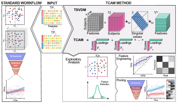
Precision medicine is a clinical approach for disease prevention, detection and treatment, which considers each individual’s genetic background, environment and lifestyle. The development of this tailored avenue has been driven by the increased availability of omics methods, large cohorts of temporal samples, and their integration with clinical data. Despite the immense progression, existing computational methods for data analysis fail to provide appropriate solutions for this complex, high-dimensional and longitudinal data. In this work we have developed a new method termed TCAM, a dimensionality reduction technique for multi-way data, that overcomes major limitations when doing trajectory analysis of longitudinal omics data. Using real-world data, we show that TCAM outperforms traditional methods, as well as state-of-the-art tensor-based approaches for longitudinal microbiome data analysis. Moreover, we demonstrate the versatility of TCAM by applying it to several different omics datasets, and the applicability of it as a drop-in replacement within straightforward ML tasks.

Introduction

Precision health and medicine aim to provide disease treatment, pre-clinical detection and prevention, while taking into consideration the individual genetic variability, environment and lifestyle. Recent developments in high-throughput methodologies enable the assessment of molecular entities from biological samples on a global scale at steadily decreasing costs, allowing to conduct biological and clinical studies at previously unfeasible magnitude, including the number of biological repetitions and molecules quantified [1]. A consequence of the increased availability of omics methods, is the possibility to conduct large-scale longitudinal studies prospectively following up the participants. In particular, longitudinal omics profiling, combined with clinical measurements, enable us to detect and understand individual changes from baseline, improving personalized health and medicine by using tailored therapies [17].

Yet, despite the surge of longitudinal multi-omics studies, the tool-set for such analyses remains limited to date, with only a handful of applicable software suitable for specific tasks [15, 20, 16]. Recently, an impressive advancement in the use of tensor factorization methods for time series analysis emerged, allowing trajectory analysis for microbiome data [14, 6] as well as neural dynamics [23]. Generally referred to as tensor component analysis (TCA) [23], these multiway dimensionality reduction methods for omics data are based on CANDECOMP/PARAFAC (CP) factorization [9, 8], which dramatically limits the ability to apply machine learning (ML) algorithms, as it does not allow for straightforward mapping of unseen data points to the reduced space. In addition, CP-based TCA requires choosing the number of components (dimensions) to be considered, since different choices may result in significantly different transformations of the data, additional uncertainties in analyzing complex information are introduced.

Here we present tcam, a new method for dimensionality reduction which provides answers the unmet need of trajectory analysis of longitudinal omics data. Our novel method is based on a cutting-edge mathematical framework (the M-product between tensor), which allows for a natural generalization of the notion of singular value decomposition (SVD) for matrices ( $2^{nd}$ order tensors) to higher order tensors [11]. We show that tcam outperforms traditional methods, as well as recent - microbiome specific - tensor factorization methods for longitudinal microbiome data analysis, both in identifying distinct trajectories between different phenotypic groups, and in highlighting significant temporal variation in bacterial entities. Furthermore, we demonstrate the versatility of tcam by applying it to a proteomics dataset, uncovering new insights that were not disclosed in the original paper, showing that our method works not only for microbiome datasets but is also applicable for a wide array of longitudinal omics data. Finally, we show that in contrast to CP-based TCA methods, our methodology can also be applied for straightforward ML tasks on omics data.

Refer to caption — Figure 1: Illustration of settings and workflow. Center rhombus describes the typical data produced in a longitudinal experiment, where $p$ dimensional samples are collected from $m$ subjects across $n$ timepoints. Fig.1a shows our new method for obtaining tensor component analysis factors from an explicit rank truncated tsvdm of the data. Figures.1b-f illustration of some prominent outcomes of tcam application, including Fig.1b ordination plot for temporal trajectories where each point approximate the complete $p$ -dimensional $n$ -timepoints long time series course of each subject in the study. Fig.1c Illustration of factor loadings distribution (top) and a summarised view for the highest magnitude contributors (bottom). The right-pointing arrow represents the applicability of factor loadings information to feature pruning, prior to univariate time-series analysis Fig.1d (Left) Pruning funnel, describing the tcam based feature selection, from the initial number of features, through the selection of features corresponding to highest magnitude loadings of factors of interest, followed by application of hypothesis testing and false discovery rate correction. (Right) Illustration of an expected outcome of the strategy - discovery of feature exhibiting significantly different temporal trends between two (or more) experimental groups. Fig.1e,f Illustration of ROC curve e and confusion matrix f, exemplifying tcam as a feature engineering step that seamlessly integrates in any standard ML workflow. Fig.1g,h Illustrates the traditional, matrix-based longitudinal ’omics data analysis workflow. Fig.1g Illustration of a collection of ordination scatterplots (such as PCA), corresponding to one possible marginalization of the data. Fig.1h Demonstration of features funnel when no pruning strategy is applied (top), and expected outcome of univariate time-series analysis when applied to all features (bottom).

Results

For the purpose of this study we utilized four different longitudinal datasets [21, 19, 18, 5], which include 16S rDNA microbiome analysis, shotgun metagenomics and proteomics data. The first study [21] investigated the reconstitution of the gut microbiome in healthy individuals following antibiotic administration, by comparing a 21 day-long probiotics supplementation (PBX), autologous fecal microbiome transplantation (aFMT) derived from a pre-antibiotics treated sample, or spontaneous recovery (CTR), using longitudinal sampling from baseline until reconstitution (n=17). The second study [5] is an interventional experiment, testing the impact of different resistant starch4 (RS4) structures on microbiome composition, in which stool samples were collected each week during a five weeks long trial (n=40). The four arms of this experiment were defined by the source of fibers: tapioca and maize groups represent sources of fermentable fibers, while potato and corn groups mostly contain fibers that are inaccessible for microbiome degradation thus, considered control groups. The third study [19] evaluated three different treatments for pediatric ulcerative colitis (UC) during a one-year follow-up, in which the stool microbiome was examined in four specific time-points (n=87). Finally, the fourth study [18] constituted a unique longitudinal experimental setting of 105 healthy volunteers to explore the influence of seasons in biological processes. To this aim, the authors performed immune profiling, proteomics, metabolomics, transcriptomics and metagenomics, collecting approximately 12 samples from each participant during the time course of four years.

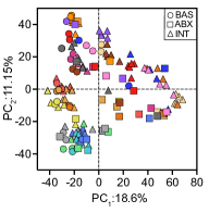
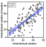
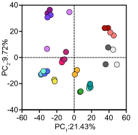
First, we sought to demonstrate the advantages of tcam over the traditional methods for microbiome analysis by applying tcam on the data from the antibiotic reconstitution project [21]. According to the original study, participants were split into three study arms (PBX, aFMT and CTR) and stool samples were collected at baseline (days 0 to 6), antibiotics treatment (days 7 to 13) and the intervention phase (days 14 to 42). We used Principal Component Analysis (PCA) as a comparison reference for our tcam method, as it constitutes a traditional gold-standard for microbiome analysis. Indeed, when we applied PCA to all of the time points, it resulted in a reduced representation that was highly affected by inter-individual differences (LABEL:fig:postabx.pca.all), while temporal intra-individual information in longitudinal data analysis is masked the inter-individual variability. The truncated representation following PCA brings little addition to the information obtained from baseline samples, as the distances between the samples across all samples are tightly correlated with the baseline distances between samples. (LABEL:fig:postabx.distance.reg and LABEL:sfig:postabx.pca.baseline). Similarly, the per-phase perspective of the data did not capture the trend of composition changes, but a mere snapshot of temporal trends (LABEL:sfig:postabx.pca.group.BAS, LABEL:sfig:postabx.pca.group.INT and LABEL:sfig:postabx.pca.group.ABX).

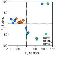
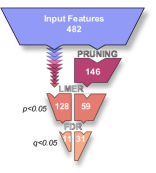
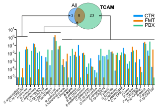
In contrast, analysis by tcam generated a temporally coherent representation of the data (LABEL:fig:postabx.tcam.factors), with only one single point representing the full trajectory of a subject throughout the entire experiment. Additionally, the tcam factor scores approximate the true distances between trajectories (Supplementary Discussion) providing an easy interpretation, which is amenable for multivariate hypothesis testing methods. We performed a PERMANOVA test to reveal significant differences between trajectories in the FMT and PBX groups (LABEL:fig:postabx.tcam.factors; p<0.05), in agreement with the original findings in the study. In addition, we highlighted the bacterial features contributing for this distinct separation between the groups, which the original study could not detect (LABEL:fig:postabx.tcam.loadings), with five of the most contributing bacteria for the significant separation between the groups were the actual probiotic species consumed by the PBX group [21]. Furthermore, we harnessed the power of tcam as part of a pruning strategy, by considering only top tcam loadings for a univariate linear mixed effect model (lmer, methods). Using our pruning strategy, we managed to discover twenty-three new bacterial features that significantly differ between the groups (two of these are probiotic species, LABEL:fig:postabx.timeser.tcam), with an overlap of eight species discovered with and without pruning (LABEL:fig:postabx.timeser.mutual). The pruning strategy failed in detection of three species, that otherwise were discovered (LABEL:fig:postabx.timeser.all and LABEL:fig:postabx.bars).

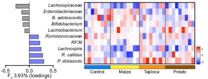
Next, we evaluated the tcam’s performance against the new state-of-the-art tensor factorization method Gemelli [14]. Unlike tcam, Gemelli is designed specifically for 16S amplicon sequencing data, as it utilizes mathematical properties that are unique to such data. For this reason, we used the RS4 interventional dataset, comparing the effect of four different types of RS4 fiber administration, tapioca, maize, corn and potato, on the microbiome composition [5]. In the original paper, the authors noticed significant changes in specific time-points in the tapioca and maize groups, but no apparent trends of changes in the microbiome composition were reported.

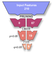
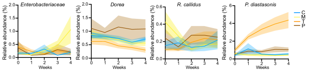
Initial analysis with Gemelli, failed to identify any significant differences between trajectories of the groups (PERMANOVA; p>0.05 LABEL:fig:fibers.gemelli.factors), however, using tcam, we were able to detect a significant trajectory for the maize group compared to all other groups, but not for the tapioca group (PERMANOVA; p<0.05, LABEL:fig:fibers.tcam). We then applied our pruning strategy, as previously described, and managed to identify four distinct bacteria featuring a statistically significant trend throughout time, not detected in the traditional methods or by Gemelli (LABEL:fig:fibers.gemelli.funnel and LABEL:fig:fibers.timeseries). Moreover, using the top loadings of $F_{3}$ (see methods), we highlighted additional features that did not pass the FDR-correction significance threshold in the previous strategy, demonstrating patterns of increasing bacteria in the form of Lachnospiraceae (p<0.05) in the maize group and P. distasonis (p<0.05) in the tapioca group (LABEL:fig:fibers.heatmap).

Taken all together, we can determine that tcam outperformed both traditional and the up-to-date longitudinal analysis workflow for time-series longitudinal trajectory analysis, identifying signals in temporal multivariate complex data that the aforementioned methods could not. Additionally, tcam performed exceptionally well as a feature pruning strategy, which reduces the features of interest and enables a sensitive detection of significant features.

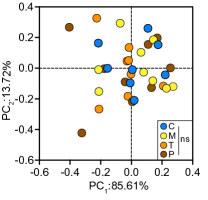
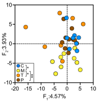
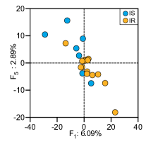
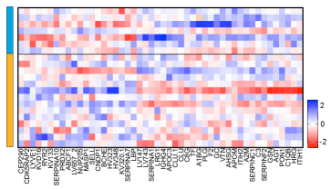
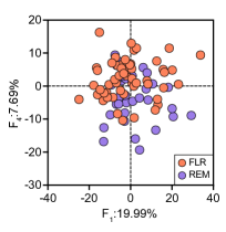
We turned to assess tcam’s applicability to general omics data, distinct from metagenomics, by applying our method to the proteomics data set [18]. In this study, twelve samples were collected from 105 healthy participants during three-years follow-up (collection of one sample every three months), and tested the seasonal trends of the microbiome, transcriptome, metabolome and proteome. We utilized a subset of this study’s data, focusing only on proteomics of individuals featuring information related to their insulin sensitivity (IS) or insulin resistance (IR). Instead of addressing seasonal patterns, which were the main focus of the original work, we addressed the differences between proteome trajectories of the IR and IS groups throughout the three-years follow-up. Using tcam, we detected a significant separation between the two groups based on $F_{1}$ (t-test; p<0.05), indicating a different trajectory of these two population across time (LABEL:fig:iris.tcam). Similar to our analysis framework above, we turned to the top loadings contributing to this signature (LABEL:fig:iris.heatmap). Among the top ranked proteins, we could easily notice angiotensinogen (AGT), which levels are associated with IS [22], paraoxonase-1 (PON1) which was found to reduce IR in mice [13], apolipoprotein-3 (APOC3), highly associated with IR [4], highlighting different trajectories for these proteins among the two groups and increasing levels of AHSG in the IS which indeed tightly associated with IS (DOI: 10.2337/diacare.29.04.06.dc05-1938)

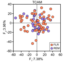
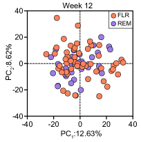
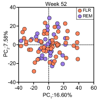
Finally, we demonstrated the predictive power unleashed by tcam from longitudinal sampling in the context of supervised ML tasks such as classification. To this aim, we utilized a 16S rDNA microbiome dataset from a study by Schirmer et. al., which includes stool samples derived from pediatric UC patients monitored for 52 weeks under three different treatments, and characterized for microbial dynamics along disease course in light of host response to each of the applied treatments [19]. When considering the complete time course, as well as, single timepoint snapshots, we found no clear separation based on the remission status of the UC patients (PERMANOVA, p>0.05; LABEL:fig:ibd.remission.projections.tcam, LABEL:fig:ibd.remission.projections.w12 and LABEL:fig:ibd.remission.projections.w52), making the task of predicting the remission status using temporal microbiome data highly challenging.

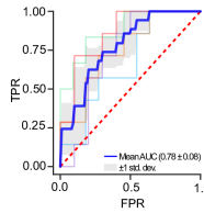
To overcome this challenge, we used tcam as a feature engineering tool in the generation of a machine learning classifier. In short, we executed five cross-validation Multi Layer Perceptron (MLP) classifier using the tcam transformed training set data, the same transformation was used in an out-of-sample extension manner to transform the validation set. The MLP had shown an impressive mean Area Under The Receiver Operating Characteristic (AUROC) of (AUROC = 0.78, LABEL:fig:ibd.tcam.roc ) for the classification of remission status. Moreover, we were able to preserve the original feature importance contribution prior to tcam, thus highlighting key bacteria that differs between remission status; Using standard variable-importance API, we were able to pin-point specific taxa like Anaerococcus and B.fragilis whose trajectories data made the highest contribution to the decision making process (LABEL:fig:ibd.tcam.important), that could not have been identified using a per time-point comparison as done in the original paper. To validate the tcam-based feature importance results, we then applied tcam on the same dataset, while taking into account only the top %5 ranked features discovered for the MLP classifier pipeline. From this reduced view, we were able to identify clustering according to remission states (LABEL:fig:ibd.pruned.tcam), validating the power of tcam classification and the preservation of feature importance scores(LABEL:fig:abundances.important.features).

We next compared the performances of the MLP tcam pipeline with those of an MLP pipeline with PCA on single time points of week 12 and week 52 (see Methods), changing only the feature engineering step while using a fixed MLP architecture. Indeed, as we expected, tcam outperformed PCA as a feature engineering technique, with both weeks 12 and 52, displaying a lower mean AUROC than tcam based workflow (W12=0.61,W52=0.68, LABEL:fig:ibd.roc.w12 and LABEL:fig:ibd.roc.w52).

Overall, in this section, we demonstrated the utility of tcam across multi-omics data and as an integral part of ML pipelines. In both scenarios we were able to show that the application of tcam had a unique added value over the traditional methods for longitudinal analysis. Moreover, we displayed the ability of tcam to exploit the full power of ML tools in longitudinal datasets, as feature engineering tool, with the preservation of the original features contributions.

Discussion

In this work, we presented tcam, a novel dimensionality reduction method for longitudinal ’omics data analysis, constructed on top of solid tensor-tensor algebra innovations. We demonstrated that tcam outperforms traditional and state-of-the-art methods for longitudinal analysis dimensionality reduction, both in terms of signature detection and by pruning for meaningful features. In addition, we showed that tcam is applicable to diverse omics types, including amplicon and shotgun sequencing as well as proteomics. Furthermore, unlike other tensor factorization methods, tcam entertains a natural out-of-sample extension formula, making it suitable for prediction tasks in complex experimental designs as a drop-in feature engineering utility within ML workflows. We have showed that we can preserve the feature importance contribution of the original features, even when tcam is applied.

To our knowledge tcam is the first tensor component analysis framework that is guarantied, within the specific choice of domain transformation, to maximize the variance of the latent representation while keeping the distortion minimal. Thus, tcam is amenable for traditional downstream applications often used in biological data analysis, such as multivariate hypothesis testing and ML workflows.

While tcam proves to be an extremely useful tool for all longitudinal analysis experimental designs, it relies on a fully sampled cohorts, where all participants provide a comparable number of samples and at similar time points in order to extract insightful biological signatures. Prior to usage of tcam, a user will have to complete the missing time points by any method he chooses, as we have done throughout this study (see methods).

Looking forward, the mathematical properties of tcam are supposed to enable us not only to perform a trajectory analysis across time, but also in a spatial manner across a geographical landscape. Moreover, it is possible to employ a tcam decomposition on higher order tensors, allowing for better understanding of even more complex experimental designs, such as incorporation of space and time together.

Overall, this novel approach answers the important unmet need of longitudinal ’omics data analysis tool-kits that enable trajectory analysis, and is available ¹¹1https://github.com/UriaMorP/mprod_package to the wide community as a simple, one-stop-shop Python implementation, that is compatible with the highly popular scikit-learn package. We hope that the application of tcam could help derive deep insights from large-scale, longitudinal and multi-omics data thus promoting personalized medicine, leading to the development of tailored treatments and preventive strategies for human diseases.

Acknowledgments

E.E. is supported by the Leona M. and Harry B. Helmsley Charitable Trust, Adelis Foundation, Pearl Welinsky Merlo Scientific Progress Research Fund, Park Avenue Charitable Fund, Hanna and Dr. Ludwik Wallach Cancer Research Fund, Daniel Morris Trust, Wolfson Family Charitable Trust and Wolfson Foundation, Ben B. and Joyce E. Eisenberg Foundation, White Rose International Foundation, Estate of Malka Moskowitz, Estate of Myron H. Ackerman, Estate of Bernard Bishin for the WIS-Clalit Program, Else Kröener-Fresenius Foundation, Jeanne and Joseph Nissim Center for Life Sciences Research, A. Moussaieff, M. de Botton, Vainboim family, A. Davidoff, the V. R. Schwartz Research Fellow Chair and by grants funded by the European Research Council, Israel Science Foundation, Israel Ministry of Science and Technology, Israel Ministry of Health, Helmholtz Foundation, Garvan Institute of Medical Research, European Crohn’s and Colitis Organization, Deutsch-Israelische Projektkooperation, IDSA Foundation and Wellcome Trust. E.E. is the incumbent of the Sir Marc and Lady Tania Feldmann Professorial Chair, a senior fellow of the Canadian Institute of Advanced Research and an international scholar of the Bill & Melinda Gates Foundation and Howard Hughes Medical Institute. H.A. is supported by the Israel Science Foundation, US-Israel Binational Science Foundation, and IBM Faculty Award. This research was partially supported by the Israeli Council for Higher Education (CHE) via the Weizmann Data Science Research Center.

Author contribution

U.M. conceived the study, established theoretical results, wrote the software package, analyzed the data, generated the figures and wrote the manuscript; Y.C. and R.V.-M. analyzed the data, gave biologically and clinically meaningful interpretation for the results, generated the figures and wrote the manuscript; D.K. assisted with data analysis and biological interpretation, wrote the manuscript; E.E. conceived the study, mentored the participants and wrote the manuscript; H.A. conceived the study, supervised the theoretical aspects, mentored the participants and wrote the manuscript.

Competing interest statement

E.E. is a scientific founder of DayTwo and BiomX, and a payed consultant to Roots GmbH. H.A. is an inventor of U.S. patent US10771088B1 which discloses the TSVDM decomposition which is the basis for tcam. U.S. patent US10771088B1 is assigned to Tel Aviv Yafo University, International Business Machines Corp and Tufts University. Inventors are Lior Horesh, Misha E. Kilmer, H.A., and Elizabeth Newman. The remaining authors declare no competing interests. U.M., Y.C., R.V.-M. and D.K. do not have any financial or non-financial competing interest.

Code and data availability

The code for the analysis presented in the paper can be found in the Github repository ²²2https://github.com/UriaMorP/tcam_analysis_notebooks. No new data was generated in this study.

Methods

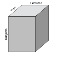
A real tensor of order- $N$ , denoted by $\boldsymbol{\mathscr{A}}\in\mathbb{R}^{d_{1}\times d_{2}\times\cdots\times d_{N}}$ , is a multi-dimensional array with real entries indexed by $N$ -tuples. For example, the $i_{1},i_{2},\dots,i_{N}$ entry of $\boldsymbol{\mathscr{A}}$ is denoted by $\boldsymbol{\mathscr{A}}_{i_{1},i_{2},\dots,i_{N}}$ . In this paper, we consider $3^{rd}$ order tensors $\boldsymbol{\mathscr{A}}\in\mathbb{R}^{m\times p\times n}$ holding data from $p$ -dimensional samples, collected from $m$ subjects across $n$ time-points. The size of $p$ is determined by the number of features measured in the ’omics method being used, it can be the number of observed bacterial species in metagenomics sequencing or the number of genes in transcriptomics etc. We use Matlab notations for slicing and indexing of tensors, e.g., $\boldsymbol{\mathscr{A}}_{i,:,:}\in\mathbb{R}^{1\times p\times n}$ denotes the $i^{th}$ horizontal slice of $\boldsymbol{\mathscr{A}}$ , which may be considered as a $p\times n$ matrix.

The mean sample of a tensor $\boldsymbol{\mathscr{A}}$ , is defined as $\bar{\boldsymbol{\mathscr{A}}}=1/m\sum_{i=1}^{m}\boldsymbol{\mathscr{A}}_{i,:,:}\in\mathbb{R}^{1\times p\times n}$ . A tensor $\boldsymbol{\mathscr{A}}$ is in mean-deviation form (MDF), if $\|\bar{\boldsymbol{\mathscr{A}}}\|_{F}^{2}=0$ , where $\|\cdot\|_{F}$ denotes the Frobenius norm: $\|\boldsymbol{\mathscr{A}}\|_{F}^{2}=\sum_{k,j,i}\boldsymbol{\mathscr{A}}_{k,j,i}$ . Any tensor $\boldsymbol{\mathscr{A}}$ can be centered to MDF by subtracting its mean sample from each horizontal slice.

Given a non-singular $n\times n$ matrix $\mathbf{M}$ , the tubal singular value decomposition with respect to the the $\star_{{\scriptscriptstyle{\mathbf{M}}}}$ -product (tsvdm) of $\boldsymbol{\mathscr{A}}$ is written as $\boldsymbol{\mathscr{A}}=\boldsymbol{\mathscr{U}}\star_{{\scriptscriptstyle{\mathbf{M}}}}\boldsymbol{\mathscr{S}}\star_{{\scriptscriptstyle{\mathbf{M}}}}\boldsymbol{\mathscr{V}}^{\mathbf{T}}$ where $\star_{{\scriptscriptstyle{\mathbf{M}}}}$ denotes the tensor-tensor product (Refer to [11] for original definitions, and Supplementary Discussion for details). Throughout this study, we considered $\mathbf{M}$ defined by the discrete cosine transform (DCT).

Given a tensor $\boldsymbol{\mathscr{A}}$ in MDF, the tcam of $\boldsymbol{\mathscr{A}}$ is defined by a scores matrix $\mathbf{Z}\in\mathbb{R}^{m\times pn}$ whose $(\ell,h)$ entry is $(\widehat{\boldsymbol{\mathscr{A}}\star_{{\scriptscriptstyle{\mathbf{M}}}}\boldsymbol{\mathscr{V}}})_{\ell,\mathbf{r}_{h,1},\mathbf{r}_{h,2}}$ , and a $np\times p$ loadings matrix $\mathbf{V}$ with entries $\mathbf{V}_{h,j}=\widehat{\boldsymbol{\mathscr{V}}}_{\mathbf{r}_{h,1},j,\mathbf{r}_{h,2}}$ . The notation $\widehat{\boldsymbol{\mathscr{X}}}$ denotes the domain transform of a tensor $\boldsymbol{\mathscr{X}}$ and $\mathbf{r}=\{(\mathbf{r}_{h,1},\mathbf{r}_{h,2})\}_{h=1}^{pn}$ is an ordered collection of tuples such that $\widehat{\boldsymbol{\mathscr{S}}}_{\mathbf{r}_{1,1},\mathbf{r}_{1,1},\mathbf{r}_{1,2}}\geq\widehat{\boldsymbol{\mathscr{S}}}_{\mathbf{r}_{2,1},\mathbf{r}_{2,1},\mathbf{r}_{2,2}}\geq\cdots\geq\widehat{\boldsymbol{\mathscr{S}}}_{\mathbf{r}_{np,1},\mathbf{r}_{np,1},\mathbf{r}_{np,2}}$ . Each row of the factors matrix represents the $p$ -dimensional time-series (trajectory) of each subject, while the loadings matrix measures the contribution - magnitude and direction - of each of the $p$ ’omics features to each of the tcam factors across samples. Refer to Supplementary Discussion for formal definitions, construction and mathematical optimality guarantees.

Excluding MDF, the tcam makes no assumptions on the data, making it suitable for any choice of normalization method. Unless stated otherwise, data were normalized to form log2 folds from baseline (LFB ); for experiment with timepoints $t_{1},\dots,t_{n}$ , where $t_{1}...t_{j}$ are considered the baseline samples. Let $s_{\ell 1},...,s_{\ell n}$ denote the samples collected from subject $\ell$ . The LFB transformed data $\hat{s}_{\ell 1},...,\hat{s}_{\ell n}$ is defined by $\hat{s}_{\ell k}\coloneqq\log_{2}(s_{\ell k}/\bar{s_{\ell}})$ where $\bar{s_{\ell}}$ is the mean of subject $\ell$ ’s baseline samples: $s_{\ell 1},...,s_{\ell j}$ .

Data processing

All tcam were computed on MDF of the data. The pre-processing and analysis steps taken vary between datasets and are listed below. Fine details are described in the provided code ³³3https://github.com/UriaMorP/tcam_analysis_notebooks.

Post antibiotics reconstitution

Shotgun metagenomics sequencing data of stool samples was downloaded from ENA (project accession number: PRJEB28097). QC filtration and read trimming was done using fastp, followed by removal of reads mapped to human genome by bowtie2 mapper. MetaPhlan3 was used for taxonomic assignment of the reads. For the analysis, we included the timepoints with missing samples of no more than 2 subjects, allowing for single day deviation in any direction. Subjects without at least one sample in each phase of the experiment (baseline, antibiotics, intervention) were excluded. Relative abundance values were capped at $10^{-6}$ and features with maximal values less then $10^{-6}$ were omitted. For the analysis using tcam, data from each participant were LFB transformed. PERMANOVA was computed using truncated distance matrices reconstructed using the minimal number of components (either tcam or PCA) such that the truncation accounts for at least 20% of the total variation in the data. Feature selection for univariate time-series analysis was done by taking the 0.75 quantile of loadings norm computed for the factors demonstrating significant univariate difference (ANOVA). Univariate time-series analysis was performed using lmer.

Dietary fiber intervention

16S rDNA sequencing data and metadata from this study [5] were downloaded from ENA (project accession number: PRJNA560950). Overlapping paired-end FASTQ files of 16S amplicon sequencing data were matched and analyzed using the Qiime2 pipeline (q2cli version 2021.4.0) [2]. Poor quality bases were trimmed, sequences were denoised and binned to amplicon sequence variants (ASVs) using the dada2 plugin for Qiime2 [3]. Taxonomic assignment was performed using naive Bayes feature classifier and Greengenes 13_8 database. Gemelli method [14] was run using raw counts and default parameters. For the analysis using tcam method, relative abundance values were capped at $10^{-3}$ , features with maximal values less then $10^{-3}$ were omitted and data from each participant were LFB transformed. PERMANOVA was computed using distance matrices reconstructed with all components (either tcam or PCA). Feature selection for univariate time-series analysis was done by taking the 0.75 quantile of loadings norm computed for the factors demonstrating significant univariate difference (ANOVA). Univariate time-series analysis was performed using lmer.

Pediatric ulcerative colitis

Sample-specific metadata and final microbial OTU relative abundances were acquired from [19]. Subjects without at least one sample in each timepoint of the experiment (0, 4, 12, 52) were excluded. Relative abundance values were capped at $10^{-4}$ , features with maximal values less then $10^{-4}$ were omitted and data from each participant were LFB transformed. To study differences in temporal microbiome composition between the three treatment groups, PERMANOVA was computed using distance matrices reconstructed with all components. A multilayer perceptron (MLP) with single 1000 neuron wide hidden layer was trained to predict treatment groups (5ASA, CS-Oral and CS-IV) using the minimal number of tcam factors such that at least 90% of the variation in the data is explained by the factors. On the other hand,a similar MLP architecture was trained to predict the combined treatment groups (5ASA, CS), using the minimal number of tcam factors such that at least 80% of the variation in the data is explained by the factors. Similarly, an MLP with single 1000 neuron wide hidden layer was trained to predict remission state using the minimal number of tcam factors such that at least 80% of the variation in the data is explained by the factors. The same MLP architecture was trained using log2 fold changes of weeks 12 and 52 to the baseline.

Identification of insulin resistance using longitudinal proteomics

Proteomics data and metadata were downloaded from https://figshare.com/articles/dataset/Multi_Omics_Seasonal_RData/12376508. Three years duration was stratified to trimesters, and repeated samples of the same participant within a trimester were median aggregated. Subjects lacking measurements in more than a single trimester were omitted from the analysis. Missing timepoints filled via linear interpolation or forward/backward filled in case of missing last/first trimester. The first year was considered as “baseline". Since proteomics data contain negative values, the data for each subject was shifted by the median baseline measurements for that subject.

1 Supplementary Figures

{supfigure}

[ph!]

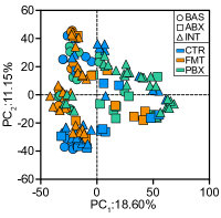
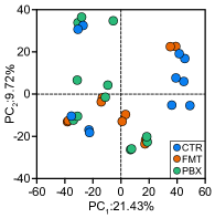
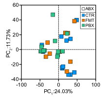
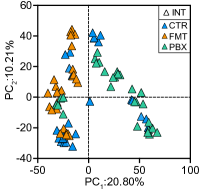
Comparison of tcam with existing matrix based methods for exploratory analysis LABEL:sfig:postabx.pca.baseline PCA plot of baseline timepoints, 1-2 samples per each subjects. Points are colored according to participant. LABEL:sfig:postabx.pca.group PCA plot of all timepoints. Points are colored according to group. LABEL:sfig:postabx.pca.group.BAS, LABEL:sfig:postabx.pca.group.ABX and LABEL:sfig:postabx.pca.group.INT PCA plot of baseline, antibiotics, and intervention phases respectively. Points are colored according to group

{supfigure}

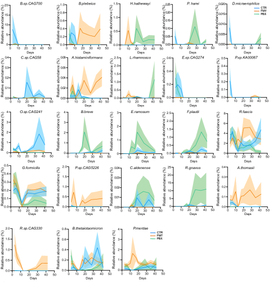
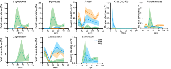
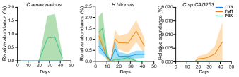
Comparison of discovery rates between naive time-series analysis and tcam based pruning LABEL:fig:postabx.timeser.tcam Time series of relative abundance levels for features discovered only when pruning the features. LABEL:fig:postabx.timeser.all and LABEL:fig:postabx.timeser.mutual Time series of relative abundance levels for features discovered when no pruning scheme is used (top) and by both methods (bottom). {supfigure}[ph!]

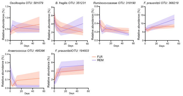
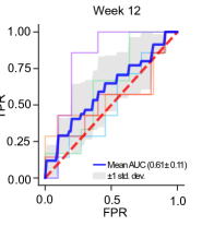
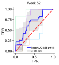
tcam analysis on pediatric UC patients. LABEL:fig:ibd.remission.projections.tcam, LABEL:fig:ibd.remission.projections.w12 and LABEL:fig:ibd.remission.projections.w52 Scatter plots for 2 leading factors of tcam for the whole dataset (LABEL:fig:ibd.remission.projections.tcam); PCA computed for log2 ratio of week 12 and baseline (LABEL:fig:ibd.remission.projections.w12); PCA computed for log2 ratio of week 52 and baseline (LABEL:fig:ibd.remission.projections.w52). Points are colored according to remission (REM) and flare (FLR) status. LABEL:fig:abundances.important.features Time series of relative abundance levels, highlighting the differences in trajectories of the features contributing to the remission status classification model. LABEL:fig:ibd.roc.w12 and LABEL:fig:ibd.roc.w52 ROC curve for MLP model trained to classify remission/flare based on PCA transformed log fold change between week 12 and baseline ( LABEL:fig:ibd.roc.w12) and log fold change between week 52 and baseline ( LABEL:fig:ibd.roc.w52). ( back to text)

Supplementary Discussion

A real order- $N$ tensor $\boldsymbol{\mathscr{A}}\in\mathbb{R}^{d_{1}\times d_{2}\times...\times d_{N}}$ is an multi-dimensional array of entries⁴⁴4In pure mathematics this is actually the definition of a hypermatrix, while a tensor is an algebraic object that describes a multilinear relationship. However, in data science often the term ‘tensor’ is abused to mean a hypermatrix, and we adopt this terminology here as well.. Each of the entries of $\boldsymbol{\mathscr{A}}$ can be referred to by specifying an $N$ -tuple of numbers $(i_{1},...,i_{N})$ where $i_{k}\in\{1,2,\dots,d_{k}\}$ .

A third-order tensor $\boldsymbol{\mathscr{A}}\in\mathbb{R}^{m\times p\times n}$ can also be viewed as an $m$ elements long list of $p\times n$ matrices, each an horizontal slice of the tensor (LABEL:sfig:cartoon.horizontal.slices.full and LABEL:sfig:cartoon.horizontal.slices). This mathematical construct is appealing in the context of longitudinal studies as it enables storing the data in a way that is consistent with the data collection. One might think of $\boldsymbol{\mathscr{A}}$ as a data-structure for holding the results of an experiment during which $n$ samples were collected from $m$ participants, and each sample is characterized by $p$ features. These features may be genes in the case of RNA-seq samples, taxonomic composition of shotgun metagenomics sequencing, etc. The tensor data structure reflects not only the data points but also key relationships between them. For example, let $1\leq i\leq p$ an integer denoting the index of a certain feature, then variations of this feature across the whole cohort are obtained by fixing the second coordinate of the tensor to $i$ : $\boldsymbol{\mathscr{A}}_{:,i,:}$ ⁵⁵5Here, we are using Matlab notation, in which ‘:’ denotes the entire range of a mode, and ‘ $l:k$ ’ denotes $\{l,l+1,\dots,k\}$ .. Similarly, tracking this feature in a single timepoint $t$ is done by restriction of the last two coordinates $\boldsymbol{\mathscr{A}}_{:,i,t}$ . {supfigure}[ph!]

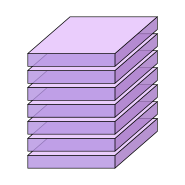
Subject centered view of $3^{rd}$ order tensor . LABEL:sfig:cartoon.horizontal.slices.full An illustration of the data structure. LABEL:sfig:cartoon.horizontal.slices The right panel presents a breakdown of the left tensor into $m$ horizontal slices that are $p\times n$ matrices. The arrangement of the same data in the form of a matrix, which has only two dimensions, would require us to make a somewhat arbitrary choice about which of the two dimensions are to be coalesced into a single dimension. For example, one might consider each individual subject as a single sample, and as such each individual will have a designated row in the data matrix, while repeated measurements of the same feature at several timepoints are treated as entirely different features, resulting in an $m\times np$ matrix. Note that by concatenating the repeated samples of each individual, we form a new feature space in which the temporal context is lost. Another option is to define samples as $p$ dimensional entities measured for each subject at all timepoints, resulting in an $nm\times p$ matrix. This formulation breaks the correspondence between data of the same individual across timepoints, as well as the data of all individuals at a single timepoint.

Continuing with the above example, if in addition we were to sample each subject at $k$ body sites (instead of one), then the number of possible ways of rearranging data in the form of a matrix would have increased to four different choices, each of which captures a different aspect of the experimental design. On the other hand, having the data in a format of tensor would only require an addition of a single mode for describing the $k$ different body sites, resulting in a fourth-order tensor in $\mathbb{R}^{m\times p\times n\times k}$ . The advantage of representing data in native tensor format as opposed to matricizing it is not unique to longitudinal studies and appears in many domains. See [11] for discussion.

In this work, we are concerned with tensor-based dimensionality reduction methods. It was previously shown, e.g. [23] and more recently [14, 6], that tensor-based dimensionality reduction methods have a potential to provide more meaningful output compared to analogous matrix-based methods. Most of these works consider the low-rank approximation in the form of a CP factorization [9]

\boldsymbol{\mathscr{A}}\approx\boldsymbol{\mathscr{A}}_{r}=\sum_{i=1}^{r}\sigma_{i}\mathbf{u}_{i}^{(1)}\circ\mathbf{u}_{i}^{(2)}\circ...\circ\mathbf{u}_{i}^{(N)}\in\mathbb{R}^{d_{1}\times...\times d_{N}},

(1)

where $\sigma_{i}$ are positive scalers, the components $\mathbf{u}_{i}^{(j)}$ are $d_{j}$ dimensional unit vectors and $\circ$ denotes the outer-product operation ( $\mathbf{u}_{i}^{(j)}\circ\mathbf{u}_{i}^{(k)}$ is a $d_{j}\times d_{k}$ matrix, while $\mathbf{u}_{i}^{(j)}\circ\mathbf{u}_{i}^{(k)}\circ\mathbf{u}_{i}^{(l)}$ is a tensor in $\mathbb{R}^{d_{j}\times d_{k}\times d_{l}}$ ). The number of terms $r$ in the above factorization denotes the maximal rank of the sought approximate $\boldsymbol{\mathscr{A}}_{r}$ of the original tensor $\boldsymbol{\mathscr{A}}$ . For brevity, we denote a CP factorization by $\boldsymbol{\mathscr{A}}_{r}=[\bf{\Sigma};\mathbf{U}_{1},...,\mathbf{U}_{N}]$ where $\bf{\Sigma}=\text{diag}(\sigma_{1},...,\sigma_{r})$ , and $\mathbf{U}_{j}$ are $d_{j}\times r$ matrices of columns that are the unit vectors $\mathbf{u}_{1}^{(j)},...\mathbf{u}_{r}^{(j)}$ . As a convention, each of the $r$ summands ( $\sigma_{i}\mathbf{u}_{i}^{(1)}\circ...\circ\mathbf{u}_{i}^{(N)}$ ) is a rank-1 tensor (for alternative definitions of tensor rank see [12]). This factorization provides an intuitive breakdown of the data which is somewhat analogous to that of a PCA for matrix data: the overall contribution of each component $\mathbf{u}_{i}^{(j)}$ to the approximation is determined by the magnitude of the corresponding scaler $\sigma_{i}$ (larger scaler implies greater contribution), and the components themselves may reflect the different modalities of the data (in the above example, $\mathbf{u}_{i}^{(1)}$ are associated with the different subjects, while $\mathbf{u}_{i}^{(2)},\mathbf{u}_{i}^{(3)}$ components are associated with features and timepoints respectively).

Computing an approximationin n the form of a CP decomposition of a given tensor $\boldsymbol{\mathscr{A}}$ is usually accomplished by solving the following optimization problem:

\displaystyle[\bf{\Sigma};\mathbf{U}_{1},...,\mathbf{U}_{N}]

\displaystyle=\text{$\arg\min$}_{\tilde{\bf{\Sigma}},\tilde{\mathbf{U}}_{1},...,\tilde{\mathbf{U}}_{N}}\|\boldsymbol{\mathscr{A}}-\sum_{i=1}^{r}\tilde{\sigma}_{i}\tilde{\mathbf{u}}_{i}^{(1)}\circ...\circ\tilde{\mathbf{u}}_{i}^{(N)}\|_{F}^{2}

(2)

where $\|\boldsymbol{\mathscr{X}}\|_{F}$ denotes the Frobenius norm of the tensor $\boldsymbol{\mathscr{X}}$ :

\|\boldsymbol{\mathscr{X}}\|_{F}^{2}=\sum_{i_{1}=1}^{d_{1}}\cdots\sum_{i_{N}=1}^{d_{N}}\boldsymbol{\mathscr{X}}_{i_{1},i_{2},\dots i_{N}}^{2}

The current gold-standard method for solving this problem is Alternating Least Squares (ALS) [12].

As discussed in the main text, it is generally hard to solve Problem (2) as it is non-convex, thus potentially having many local minimizers which are not global minima. Indeed, even the gold-standard method (ALS) is not guaranteed to find a global minimum. Moreover, given a data tensor $\boldsymbol{\mathscr{A}}$ (subjects, features and time), and its CP form approximate $\boldsymbol{\mathscr{A}}_{r}=[\bf{\Sigma};\mathbf{U}_{1},\mathbf{U}_{2},\mathbf{U}_{3}]$ , suppose that we are provided with data for a new participant $\boldsymbol{\mathscr{X}}\in\mathbb{R}^{1\times p\times n}$ , then the task of extending the current factorization to the new data tensor, which is $\boldsymbol{\mathscr{A}}$ augmented with the new sample $\boldsymbol{\mathscr{X}}$ , is far from a trivial one. Such out-of-sample extension capability is a fundamental requirement from any embedding algorithm that we wish to use as a step in a ML pipeline.

The aim of tcam is to provide a tensor-based PCA-like tool that is better than CP, in terms of ease of interpretation of the model’s outcomes and mathematical properties that ensure safe application to downstream statistical analysis and ML workflows.

Appendix A PCA

Since we strive to have to claim that tcam is ‘PCA-like’, it is useful to first present a brief definition of PCA, and discuss it characteristics. All constructions, definitions and properties presented in this section are taken from [10].

Let $\mathbf{A}\in\mathbb{R}^{m\times p}$ be a data matrix with rows $\mathbf{a}_{1},\dots,\mathbf{a}_{m}$ corresponding to $m$ samples, and assume that $\mathbf{A}$ has been centered (so the column means are zero). PCA is defined by an orthogonal linear transformation $\mathbf{W}$ transforming the rows of $\mathbf{A}$ to a new coordinates system, in which, the largest portion of variation in the data lies on the first axis (called the first principal component of $\mathbf{A}$ ), i.e. $\mathbf{z}_{1}=\mathbf{A}\mathbf{w}_{1}$ where $\mathbf{w}_{1}\in\mathbb{R}^{p}$ is the maximizer of $\mathbf{w}^{\mathbf{T}}\mathbf{A}^{\mathbf{T}}\mathbf{A}\mathbf{w}$ subjected to $\|\mathbf{w}\|_{2}^{2}=1$ . The $k^{th}$ largest portion of variation lies on the $k^{th}$ principal component of $\mathbf{A}$ , i.e.

\displaystyle\mathbf{z}_{k}=\mathbf{A}\mathbf{w}_{k},

\displaystyle\mathbf{w}_{k}=\text{argmax}_{\|\mathbf{w}\|_{2}=1}\mathbf{w}^{\mathbf{T}}{\mathbf{A}^{(k)}}^{\mathbf{T}}\mathbf{A}^{(k)}\mathbf{w}

where given the first $k-1$ principal components of $\mathbf{A}$ we define $\mathbf{A}^{(k)}=\mathbf{A}(\mathbf{I}-\sum_{i=1}^{k-1}\mathbf{w}_{i}\mathbf{w}_{i}^{\mathbf{T}})$ . The complete factorization yields the expression $\mathbf{Z}=\mathbf{A}\mathbf{W}$ , where rows of the matrix $\mathbf{Z}\in\mathbb{R}^{m\times p}$ are called the sample PC scores (the $i^{th}$ row of $\mathbf{Z}$ contains the sample PC scores of the $i^{th}$ sample $\mathbf{a}_{i}$ ). The orthogonal $p\times p$ matrix $\mathbf{W}$ is called the weight or coefficients matrix. The rank $k$ -truncated PCA of a $m\times p$ matrix $\mathbf{A}$ is defined by

\mathbf{Z}_{k}=\mathbf{A}\mathbf{W}_{k}\in\mathbb{R}^{m\times k}

(3)

where $\mathbf{W}_{k}\coloneqq[\mathbf{w}_{1},...,\mathbf{w}_{k}]$ is an $p\times k$ matrix with orthonormal rows; $\mathbf{W}_{k}^{\mathbf{T}}\mathbf{W}_{k}=\mathbf{I}_{k}$ . The $k$ -truncated PCA $\mathbf{Z}_{k}$ consists of only the first $k$ principal components.

The sample variance-covariance matrix of the collection $\{\mathbf{a}_{i}\}_{i=1}^{m}$ of $m$ , (centered) $p$ -dimensional samples $\mathbf{S}$ is given by $\mathbf{S}=(m-1)^{-1}\mathbf{A}^{\mathbf{T}}\mathbf{A}\leavevmode\nobreak\ .\leavevmode\nobreak\$

Property A.1 ([10, Chapter 2, Properties A1 and A2]).

For any integer $q=1,\dots,p$ , consider the transformation $\mathbf{y}_{i}=\mathbf{B}^{\mathbf{T}}\mathbf{a}_{i}$ , where $\mathbf{y}\in\mathbb{R}^{q}$ and $\mathbf{B}$ is a ${p\times q}$ matrix with $q$ orthonormal columns. Define $\mathbf{S}_{\mathbf{y}}=\mathbf{B}^{\mathbf{T}}\mathbf{S}\mathbf{B}\in\mathbb{R}^{q\times q}$ the variance-covariance matrix for $\mathbf{y}$ . The variance component of $\mathbf{S}_{\mathbf{y}}$ , quantified by $\operatorname{Tr}(\mathbf{S}_{\mathbf{y}})$ , is maximized when taking $\mathbf{B}=\mathbf{W}_{q}$ and minimized when $\mathbf{B}=[\mathbf{w}_{p-q},\mathbf{w}_{p-q+1},...\mathbf{w}_{p}]$

Property A.2 ([10, Chapter 3, Eq. 3.1.4, Property A3]).

$\mathbf{S}=\sum_{i=1}^{p}\lambda_{i}\mathbf{w}_{i}\mathbf{w}^{\mathbf{T}}_{i}$

Property A.3 ([10, Chapter 3, Property G4]).

Let $\tilde{\mathbf{A}}=[\mathbf{a}_{1};...;\mathbf{a}_{m}]$ be a $m\times p$ matrix of $m$ , $p$ -dimensional observations. Define $\mathbf{A}$ to be the $m\times p$ matrix whose $i^{th}$ row is $\mathbf{a}_{i}-\bar{\mathbf{a}}$ where $\bar{\mathbf{a}}=\frac{1}{m}\sum_{j=1}^{m}\mathbf{a}_{j}$ and consider the matrix $\mathbf{A}\mathbf{A}^{\mathbf{T}}\in\mathbb{R}^{m\times m}$ . The $i^{th}$ diagonal element of $\mathbf{A}\mathbf{A}^{\mathbf{T}}$ is the squared Euclidean distance of the sample $\mathbf{a}_{i}$ from the point $\bar{\mathbf{a}}$ that is the center of gravity of the points $\mathbf{a}_{1}...\mathbf{a}_{m}$ . Also, the $i,j$ entry of $\mathbf{A}\mathbf{A}^{\mathbf{T}}$ , given by $\langle\mathbf{a}_{i}-\bar{\mathbf{a}},\mathbf{a}_{j}-\bar{\mathbf{a}}\rangle$ , is the cosine of the angle between the lines joining the points $\mathbf{a}_{j}$ and $\mathbf{a}_{i}$ to $\bar{\mathbf{a}}$ , scaled by the distances of $\mathbf{a}_{j}$ and $\mathbf{a}_{i}$ from $\bar{\mathbf{a}}$ . Suppose that $\mathbf{a}_{1}...\mathbf{a}_{m}$ are projected to a $q$ -dimensional subspace using a linear orthogonal transformation $\mathbf{y}_{i}=\mathbf{B}^{\mathbf{T}}\mathbf{a}_{i}$ , and let $\mathbf{Y}\coloneqq[\mathbf{y}_{1}-\bar{\mathbf{y}};...;\mathbf{y}_{m}-\bar{\mathbf{y}}]\in\mathbb{R}^{m\times q}$ for $\bar{\mathbf{y}}=m^{-1}\sum_{j=1}^{m}\mathbf{y}_{j}\in\mathbb{R}^{q}$ . Then the choice $\mathbf{B}=\mathbf{W}_{q}$ minimizes the distortion $\|\mathbf{Y}\mathbf{Y}^{\mathbf{T}}-\mathbf{A}\mathbf{A}^{\mathbf{T}}\|_{F}^{2}$

Singular Value Decomposition.

One practical way of describing and computing PCA for a matrix $\tilde{\mathbf{A}}\in\mathbb{R}^{m\times p}$ , is using the singular value decomposition of its column centered form. Let again $\mathbf{A}$ denote the column centered form of $\tilde{\mathbf{A}}$ ,. and let $\mathbf{A}=\mathbf{U}\Sigma\mathbf{V}^{\mathbf{T}}$ be its Singular Value Decomposition (SVD). That is, $\mathbf{U}\in\mathbb{R}^{m\times m}$ and $\mathbf{V}\in\mathbb{R}^{p\times p}$ are orthonormal matrices, and $\Sigma\in\mathbb{R}^{m\times p}$ is a matrix with non-negative elements $\sigma_{1}\geq\sigma_{2}\geq...$ on its main diagonal and zeros elsewhere. The sample variance-covariance matrix $\mathbf{S}$ can rewritten as $\mathbf{S}=(m-1)^{-1}\mathbf{V}\Sigma^{\mathbf{T}}\Sigma\mathbf{V}^{\mathbf{T}}$ , thus the columns of $\mathbf{V}$ are the eigenvectors of $\mathbf{S}$ and, according to Property A.2, the coefficients in the PCA decomposition of $\tilde{\mathbf{A}}$ .

Let us denote the rank- $r$ truncated SVD of $\mathbf{A}$ by $\mathbf{A}_{r}=\mathbf{U}_{r}\Sigma_{r}\mathbf{V}^{\mathbf{T}}_{r}$ where $\mathbf{U}$ and $\mathbf{V}$ are the matrices obtained be taking the first $r$ columns of $\mathbf{U}$ and $\mathbf{V}$ respectively, and $\Sigma_{r}=\textnormal{diag}(\sigma_{1},...,\sigma_{r})$ . Suppose that the rank of $\mathbf{A}$ is greater or equal to $r$ , then the rank of $\mathbf{A}_{r}$ is exactly $r$ . This truncation of the SVD enjoys many algebraic properties, one such major result is the following Eckart-Young-Mirsky Theorem, stating that the $r$ -rank truncated SVD of a matrix is in a sense the best approximate of rank lower or equal to $r$ :

\mathbf{A}_{r}=\text{$\arg\min$}_{\tilde{\mathbf{A}},\textnormal{rank}(\tilde{\mathbf{A}})\leq r}\|\mathbf{A}-\tilde{\mathbf{A}}\|_{F}^{2}

This result directly implies Properties A.1 and A.3 of the PCA that are concerned with the maximization of the variance and minimizing the distortion of the projected configuration. Thus, we see that the SVD can be used not only as an alternative construction algorithm for the PCA, but also, due to Eckart-Young Theorem, can serve as the mathematical justification to some of the PCA’s key properties.

Appendix B Tensors component analysis

A recent work by Kilmer et. al. introduced a tensor version of the Eckart-Young Theorem [11], stating that the truncated tensor SVD is the best low rank approximate within a specified tensor-tensor product framework based on the $\star_{{\scriptscriptstyle{\mathbf{M}}}}$ -product. The $\star_{{\scriptscriptstyle{\mathbf{M}}}}$ -product operation is defined by an invertible matrix $\mathbf{M}$ , and the best low rank approximation results from [11] were established for matrices $\mathbf{M}$ that are nonzero multiple of a unitary matrix ( $\mathbf{M}^{\mathbf{T}}\mathbf{M}=\mathbf{M}\mathbf{M}^{\mathbf{T}}=c^{2}\mathbf{I}_{n}$ for some constant $c\neq 0$ ). In this work, we only consider $\mathbf{M}$ that are unitary matrices.

We construct the tcam on top the tensor SVD introduced by Kilmer et. al., and utilize Kilmer’s Eckart-Young-like result to establish tensor analogs of Properties A.1 and A.3, in the same way that matrix SVD can be used for deriving the same properties for matrices. As a prelude to our discussion, we present some key notions and operations necessary for our derivation. Elaborated introduction and discussion can be found in [11].

B.1 Tensor-tensor $\star_{{\scriptscriptstyle{\mathbf{M}}}}$ -product framework

We begin with some definitions. Let $\mathbf{M}$ be an $n\times n$ orthogonal matrix ( $\mathbf{M}\mathbf{M}^{\mathbf{T}}=\mathbf{I}_{n}=\mathbf{M}^{\mathbf{T}}\mathbf{M}$ ), and a tensor $\boldsymbol{\mathscr{A}}\in\mathbb{R}^{m\times p\times n}$ . We define the domain transform specified by $\mathbf{M}$ as $\widehat{\boldsymbol{\mathscr{A}}}\coloneqq\boldsymbol{\mathscr{A}}\times_{3}\mathbf{M}$ , where $\times_{3}\mathbf{M}$ denotes the tensor-matrix multiplication of applying $\mathbf{M}$ to each of the tensor $n$ dimensional tubal fibers ( $\boldsymbol{\mathscr{A}}_{i,j,:}$ ). The transpose of a real $m\times p\times n$ tensor $\boldsymbol{\mathscr{A}}$ with respect to $\mathbf{M}$ , denoted by $\boldsymbol{\mathscr{A}}^{\mathbf{T}}$ , is a $p\times m\times n$ tensor for which $[\widehat{\boldsymbol{\mathscr{A}}^{\mathbf{T}}}]_{:,:,i}=[\widehat{\boldsymbol{\mathscr{A}}}^{\mathbf{T}}]_{:,:,i}={[\widehat{\boldsymbol{\mathscr{A}}}]_{:,:,i}}^{\mathbf{T}}$ . Given two tensors $\boldsymbol{\mathscr{A}}\in\mathbb{R}^{m\times p\times n}$ and $\boldsymbol{\mathscr{B}}\in\mathbb{R}^{p\times l\times n}$ , the facewise tensor-tensor product of $\boldsymbol{\mathscr{A}}$ and $\boldsymbol{\mathscr{B}}$ , denoted by $\boldsymbol{\mathscr{A}}\vartriangle\boldsymbol{\mathscr{B}}$ , is the $m\times l\times n$ tensor for which $[\boldsymbol{\mathscr{A}}\vartriangle\boldsymbol{\mathscr{B}}]_{:,:,i}=\boldsymbol{\mathscr{A}}_{:,:,i}\boldsymbol{\mathscr{B}}_{:,:,i}$ .

We can now define the product The tensor-tensor $\star_{{\scriptscriptstyle{\mathbf{M}}}}$ -product of $\boldsymbol{\mathscr{A}}\in\mathbb{R}^{m\times p\times n}$ and $\boldsymbol{\mathscr{B}}\in\mathbb{R}^{p\times l\times n}$ is defined by $\boldsymbol{\mathscr{A}}\star_{{\scriptscriptstyle{\mathbf{M}}}}\boldsymbol{\mathscr{B}}\coloneqq(\widehat{\boldsymbol{\mathscr{A}}}\vartriangle\widehat{\boldsymbol{\mathscr{B}}})\times_{3}\mathbf{M}^{-1}\in\mathbb{R}^{m\times l\times n}$ . A few definitions now naturally follow. The $p\times p\times n$ identity tensor with respect to $\star_{{\scriptscriptstyle{\mathbf{M}}}}$ , is the tensor $\boldsymbol{\mathscr{I}}$ such that for any tensor $\boldsymbol{\mathscr{E}}\in\mathbb{R}^{p\times p\times n}$ it holds that $\boldsymbol{\mathscr{I}}\star_{{\scriptscriptstyle{\mathbf{M}}}}\boldsymbol{\mathscr{E}}=\boldsymbol{\mathscr{E}}=\boldsymbol{\mathscr{E}}\star_{{\scriptscriptstyle{\mathbf{M}}}}\boldsymbol{\mathscr{I}}$ . In situations where the dimensions are unclear from context, we use $\boldsymbol{\mathscr{I}}_{m}$ to denote the $m\times m\times n$ identity tensor. Two tensors $\boldsymbol{\mathscr{A}},\boldsymbol{\mathscr{B}}\in\mathbb{R}^{1\times m\times n}$ are called $\star_{{\scriptscriptstyle{\mathbf{M}}}}$ -orthogonal slices if $\boldsymbol{\mathscr{A}}^{\mathbf{T}}\star_{{\scriptscriptstyle{\mathbf{M}}}}\boldsymbol{\mathscr{B}}=\mathbf{0}$ , where $\mathbf{0}\in\mathbb{R}^{1\times 1\times n}$ is the zero tube fiber, while $\boldsymbol{\mathscr{Q}}\in\mathbb{R}^{m\times m\times n}$ is called $\star_{{\scriptscriptstyle{\mathbf{M}}}}$ -unitary if $\boldsymbol{\mathscr{Q}}^{\mathbf{T}}\star_{{\scriptscriptstyle{\mathbf{M}}}}\boldsymbol{\mathscr{Q}}=\boldsymbol{\mathscr{I}}=\boldsymbol{\mathscr{Q}}\star_{{\scriptscriptstyle{\mathbf{M}}}}\boldsymbol{\mathscr{Q}}^{\mathbf{T}}$ .

The following definition is new, and is important for stating the PCA-like properties of tcam.

Definition B.1.

A tensor $\boldsymbol{\mathscr{B}}\in\mathbb{R}^{p\times k\times n}$ is said to be a pseudo $\star_{{\scriptscriptstyle{\mathbf{M}}}}$ -unitary tensor (or pseudo $\star_{{\scriptscriptstyle{\mathbf{M}}}}$ -orthogonal) if $\boldsymbol{\mathscr{B}}^{\mathbf{T}}\star_{{\scriptscriptstyle{\mathbf{M}}}}\boldsymbol{\mathscr{B}}$ is f-diagonal (i.e., all frontal slices are diagonal), and all frontal slices of $(\boldsymbol{\mathscr{B}}^{\mathbf{T}}\star_{{\scriptscriptstyle{\mathbf{M}}}}\boldsymbol{\mathscr{B}})\times_{3}\mathbf{M}$ are diagonal matrices with entries that are either ones or zeros.

B.2 The tsvdm

With the $\star_{{\scriptscriptstyle{\mathbf{M}}}}$ -product framework set-up, it is now possible to introduce the tensor singular value decomposition (tsvdm). Let $\boldsymbol{\mathscr{A}}\in\mathbb{R}^{m\times p\times n}$ be a real tensor, then is possible to write the full tubal singular value decomposition of $\boldsymbol{\mathscr{A}}$ as $\boldsymbol{\mathscr{A}}=\boldsymbol{\mathscr{U}}\star_{{\scriptscriptstyle{\mathbf{M}}}}\boldsymbol{\mathscr{S}}\star_{{\scriptscriptstyle{\mathbf{M}}}}\boldsymbol{\mathscr{V}}^{\mathbf{T}}$ , where $\boldsymbol{\mathscr{U}},\boldsymbol{\mathscr{V}}$ are $m\times m\times n$ and $p\times p\times n$ $\star_{{\scriptscriptstyle{\mathbf{M}}}}{\textnormal{-unitary}}$ tensors respectively, and $\boldsymbol{\mathscr{S}}\in\mathbb{R}^{m\times p\times n}$ is an f-diagonal tensor, that is, a tensor whose frontal slices ( $\boldsymbol{\mathscr{S}}_{:,:,i}$ ) are matrices with zeros outside their main diagonal (see [11] for additional details). We use the notation $\hat{\sigma}_{j}^{(i)}$ do denote the $j^{th}$ largest singular value on the $i^{th}$ lateral face of $\widehat{\boldsymbol{\mathscr{S}}}$ : $\hat{\sigma}_{j}^{(i)}\coloneqq\widehat{\boldsymbol{\mathscr{S}}}_{j,j,i}$ .

The tsvdm construction makes it possible to expand the concept of tensor-rank discussed earlier. The t-rank of $\boldsymbol{\mathscr{A}}$ is the number of nonezero tubes of $\boldsymbol{\mathscr{S}}$ : $r=|\left\{i=1,\dots,n\leavevmode\nobreak\ ;\leavevmode\nobreak\ \|\boldsymbol{\mathscr{S}}_{i,i,:}\|_{F}^{2}>0\right\}|$ . Additionally, the multi-rank of $\boldsymbol{\mathscr{A}}$ under $\star_{{\scriptscriptstyle{\mathbf{M}}}}$ , denoted by the vector $\boldsymbol{\rho}\in\mathbb{N}^{n}$ whose $i^{th}$ entry is $\boldsymbol{\rho}_{i}=\operatorname{rank}(\widehat{\boldsymbol{\mathscr{A}}}_{:,:,i})$ , and the implicit rank under $\star_{{\scriptscriptstyle{\mathbf{M}}}}$ of a tensor $\boldsymbol{\mathscr{A}}$ with multi-rank $\boldsymbol{\rho}$ under $\star_{{\scriptscriptstyle{\mathbf{M}}}}$ is $r=\sum_{i=1}^{n}\boldsymbol{\rho}_{i}$ .

The definitions of tensor t-rank and multi-rank under $\star_{{\scriptscriptstyle{\mathbf{M}}}}$ also make it possible to define tsvdm rank truncation with respect to these ranks. The tensor $\boldsymbol{\mathscr{A}}^{(q)}=\boldsymbol{\mathscr{U}}_{:,1:q,:}\star_{{\scriptscriptstyle{\mathbf{M}}}}\boldsymbol{\mathscr{S}}_{1:q,1:q,:}\star_{{\scriptscriptstyle{\mathbf{M}}}}{\boldsymbol{\mathscr{V}}_{:,1:q,:}}^{\mathbf{T}}$ denotes the t-rank $q$ truncation of $\boldsymbol{\mathscr{A}}$ under $\star_{{\scriptscriptstyle{\mathbf{M}}}}$ , while multi-rank $\boldsymbol{\rho}$ truncation of $\boldsymbol{\mathscr{A}}$ under $\star_{{\scriptscriptstyle{\mathbf{M}}}}$ is given by the tensor $\boldsymbol{\mathscr{A}}_{\boldsymbol{\rho}}$ for which $\widehat{\boldsymbol{\mathscr{A}}_{\boldsymbol{\rho}}}_{:,:,i}=\widehat{\boldsymbol{\mathscr{U}}}_{:,1:\boldsymbol{\rho}_{i},i}\widehat{\boldsymbol{\mathscr{S}}}_{1:\boldsymbol{\rho}_{i},1:\boldsymbol{\rho}_{i},i}{\widehat{\boldsymbol{\mathscr{V}}}_{:,1:\boldsymbol{\rho}_{i},i}}^{\mathbf{T}}$ . Note that for t-rank truncation the $\boldsymbol{\mathscr{U}}$ and $\boldsymbol{\mathscr{V}}$ factors are $\star_{{\scriptscriptstyle{\mathbf{M}}}}$ -orthogonal, while for multi-rank truncation they are only pseudo $\star_{{\scriptscriptstyle{\mathbf{M}}}}$ -orthogonal.

The Eckart-Young-like result obtained by Kilmer et. al. states that $\boldsymbol{\mathscr{A}}^{(q)}$ and $\boldsymbol{\mathscr{A}}_{\boldsymbol{\rho}}$ are the ‘best t/multi-rank $q,\boldsymbol{\rho}$ ’ approximations of $\boldsymbol{\mathscr{A}}$ respectively, where ‘best’ refers to entrywise squared error, i.e. the Frobenius norm of the error. In other words, $\boldsymbol{\mathscr{A}}^{(qk)}$ and $\boldsymbol{\mathscr{A}}_{\boldsymbol{\rho}}$ are the global minimizers of $\|\boldsymbol{\mathscr{A}}-\boldsymbol{\mathscr{B}}\|_{F}^{2}$ for $\boldsymbol{\mathscr{B}}$ with t-rank $q$ (respectively, multi-rank $\boldsymbol{\rho}$ ) under $\star_{{\scriptscriptstyle{\mathbf{M}}}}$ of the same dimensions as $\boldsymbol{\mathscr{A}}$ .

Let $\boldsymbol{\mathscr{A}}=\boldsymbol{\mathscr{U}}\star_{{\scriptscriptstyle{\mathbf{M}}}}\boldsymbol{\mathscr{S}}\star_{{\scriptscriptstyle{\mathbf{M}}}}\boldsymbol{\mathscr{V}}^{\mathbf{T}}\in\mathbb{R}^{m\times p\times n}$ , we will use $j_{1},\dots,j_{np}$ and $i_{1},\dots,i_{np}$ to denote the indexes of the non-zeros of $\widehat{\boldsymbol{\mathscr{S}}}$ ordered in decreasing order. That is

\hat{\sigma}_{\ell}\coloneqq\hat{\sigma}_{j_{\ell}}^{(i_{\ell})}

(4)

where $\hat{\sigma}_{1}\geq\hat{\sigma}_{2}\geq\dots\geq\hat{\sigma}_{np}$ .

In this work, we consider truncation with respect to the explicitly given implicit rank under $\star_{{\scriptscriptstyle{\mathbf{M}}}}$ . For $q=1,\dots,pn$ , the explicit rank- $q$ truncation under $\star_{{\scriptscriptstyle{\mathbf{M}}}}$ of $\boldsymbol{\mathscr{A}}$ is the tensor $\boldsymbol{\mathscr{A}}_{\boldsymbol{\rho}}$ of multi-rank $\boldsymbol{\rho}$ under $\star_{{\scriptscriptstyle{\mathbf{M}}}}$ where

\boldsymbol{\rho}_{i}=\max\{j=1,\dots,p\leavevmode\nobreak\ |\leavevmode\nobreak\ (j,i)\in\{(j_{1},j_{1}),\dots,(j_{q},i_{q})\}\}\leavevmode\nobreak\ \leavevmode\nobreak\ .

(5)

In words, we keep the $q$ top singular values of any frontal slice of $\widehat{\boldsymbol{\mathscr{S}}}$ , and zero out the rest. Note that the explicit rank- $q$ truncation is not always uniquely defined by $q$ since ties between singular values result in multiple possible choices for the multi-rank $\boldsymbol{\rho}$ . However, all explicit-rank $q$ truncations are equivalent in that they produce identical reconstruction errors. Indeed, let $\boldsymbol{\mathscr{A}}_{\boldsymbol{\rho}}$ be a multi-rank $\boldsymbol{\rho}$ truncation of $\boldsymbol{\mathscr{A}}$ , implied by target explicit rank $q$ , then $\|\boldsymbol{\mathscr{A}}-\boldsymbol{\mathscr{A}}_{\boldsymbol{\rho}}\|_{F}^{2}=\sum_{{\ell=q+1}}^{p\cdot n}\hat{\sigma}_{\ell}^{2}$ , meaning that the reconstruction error remains the same for any choice of multi-rank $\boldsymbol{\rho}$ in eq. 5. Furthermore, given the definition of explicit rank truncation, we get the following.

Claim B.1.

Suppose that $\mathbf{M}$ is a unitary matrix. Let $\boldsymbol{\mathscr{A}}\in\mathbb{R}^{m\times p\times n}$ , with a full tsvdm $\boldsymbol{\mathscr{A}}=\boldsymbol{\mathscr{U}}\star_{{\scriptscriptstyle{\mathbf{M}}}}\boldsymbol{\mathscr{S}}\star_{{\scriptscriptstyle{\mathbf{M}}}}\boldsymbol{\mathscr{V}}^{\mathbf{T}}$ , and $\boldsymbol{\rho}=[\boldsymbol{\rho}_{1},\dots,\boldsymbol{\rho}_{n}]$ be the multi rank defined by explicit rank- $q$ truncation of $\boldsymbol{\mathscr{A}}$ in eq. 5. Let $\boldsymbol{\mathscr{A}}_{\boldsymbol{\rho}}=\boldsymbol{\mathscr{U}}_{\boldsymbol{\rho}}\star_{{\scriptscriptstyle{\mathbf{M}}}}\boldsymbol{\mathscr{S}}_{\boldsymbol{\rho}}\star_{{\scriptscriptstyle{\mathbf{M}}}}\boldsymbol{\mathscr{V}}^{\mathbf{T}}_{\boldsymbol{\rho}}\in\mathbb{R}^{m\times p\times n}$ , the multi-rank $\boldsymbol{\rho}$ truncation of $\boldsymbol{\mathscr{A}}$ , then $\boldsymbol{\mathscr{A}}_{\boldsymbol{\rho}}$ is the best implicit rank- $q$ approximation of $\boldsymbol{\mathscr{A}}$ .

Proof.

Let $\boldsymbol{\varphi}=[\boldsymbol{\varphi}_{1},\dots,\boldsymbol{\varphi}_{n}]$ be a multi-rank such that $\sum_{i=1}^{n}\boldsymbol{\varphi}_{i}=q$ . Then $\boldsymbol{\mathscr{A}}_{\boldsymbol{\varphi}}=\boldsymbol{\mathscr{U}}_{\boldsymbol{\varphi}}\star_{{\scriptscriptstyle{\mathbf{M}}}}\boldsymbol{\mathscr{S}}_{\boldsymbol{\varphi}}\star_{{\scriptscriptstyle{\mathbf{M}}}}\boldsymbol{\mathscr{V}}^{\mathbf{T}}_{\boldsymbol{\varphi}}\in\mathbb{R}^{m\times p\times n}$ is the best multi-rank $\boldsymbol{\varphi}$ approximation of $\boldsymbol{\mathscr{A}}$ . Let the tuples $(\tilde{j}_{1},\tilde{i}_{1}),\dots,(\tilde{j}_{q},\tilde{i}_{q})$ denote an ordering of the singular values $\{\hat{\sigma}_{j}^{(i)}\}$ for $i=1,\dots,n$ and $j=1,\dots,\boldsymbol{\varphi}_{i}$ , such that $\hat{\sigma}_{\tilde{1}}\geq\hat{\sigma}_{\tilde{2}}\geq\dots\geq\hat{\sigma}_{\tilde{q}}$ where $\hat{\sigma}_{\tilde{\ell}}=\hat{\sigma}_{\tilde{j}_{\ell}}^{(\tilde{i}_{\ell})}$ . Then, by construction of $\hat{\sigma}_{\ell}$ in eq. 4, we have that $\hat{\sigma}_{\ell}\geq\hat{\sigma}_{\tilde{\ell}}$ for all $\ell=1,\dots,q$ , hence $\sum_{h=1}^{q}\hat{\sigma}_{\tilde{h}}^{2}\leq\sum_{h=1}^{q}\hat{\sigma}_{h}^{2}$ .

Now, we have that

	$\displaystyle\\|\boldsymbol{\mathscr{A}}-\boldsymbol{\mathscr{A}}_{\boldsymbol{\varphi}}\\|_{F}^{2}$	$\displaystyle=\sum_{i=1}^{n}\sum_{j=1}^{p}(\hat{\sigma}_{j}^{(i)})^{2}-\sum_{i=1}^{n}\sum_{j=1}^{\boldsymbol{\varphi}_{i}}(\hat{\sigma}_{j}^{(i)})^{2}$
		$\displaystyle=\sum_{h=1}^{pn}\hat{\sigma}_{h}^{2}-\sum_{h=1}^{q}\hat{\sigma}_{\tilde{h}}^{2}$
		$\displaystyle\geq\sum_{h=1}^{pn}\hat{\sigma}_{h}^{2}-\sum_{h=1}^{q}\hat{\sigma}_{h}^{2}$
		$\displaystyle=\\|\boldsymbol{\mathscr{A}}-\boldsymbol{\mathscr{A}}_{\boldsymbol{\rho}}\\|_{F}^{2}$

Thus, we established that the best implicit rank $q$ approximation of $\boldsymbol{\mathscr{A}}$ , is the tensor $\boldsymbol{\mathscr{A}}_{\boldsymbol{\rho}}$ with multi-rank $\boldsymbol{\rho}$ implied by explicit rank $q$ truncation of $\boldsymbol{\mathscr{A}}$ . ∎

We also note that for the explicit rank- $q$ truncation of $\boldsymbol{\mathscr{A}}$ , it holds that

\|\boldsymbol{\mathscr{A}}_{\boldsymbol{\rho}}\|_{F}^{2}=\sum_{h=1}^{q}\hat{\sigma}_{h}^{2}

(6)

where $\hat{\sigma}_{h}$ is defined by eq. 4.

B.3 A PCA-like tensor decomposition

The following construction was first presented in [7]. Short presentation of the objects we are concerned with are be followed by novel results regarding their algebraic and geometric properties. For extended discussion, see [7, 11]

Let $\boldsymbol{\mathscr{A}}=\boldsymbol{\mathscr{U}}\star_{{\scriptscriptstyle{\mathbf{M}}}}\boldsymbol{\mathscr{S}}\star_{{\scriptscriptstyle{\mathbf{M}}}}\boldsymbol{\mathscr{V}}^{\mathbf{T}}\in\mathbb{R}^{m\times p\times n}$ in mean deviation form (see Methods section), and consider the following expressions [7]:

\boldsymbol{\mathscr{Z}}=\boldsymbol{\mathscr{A}}\star_{{\scriptscriptstyle{\mathbf{M}}}}\boldsymbol{\mathscr{V}}

(7)

and

\boldsymbol{\mathscr{Z}}_{\boldsymbol{\rho}}\coloneqq\boldsymbol{\mathscr{A}}\star_{{\scriptscriptstyle{\mathbf{M}}}}\boldsymbol{\mathscr{V}}_{\boldsymbol{\rho}}

(8)

where the tensor $\boldsymbol{\mathscr{V}}_{\boldsymbol{\rho}}\in\mathbb{R}^{p\times p\times n}$ is obtained from explicit rank $q$ truncated tsvdm of $\boldsymbol{\mathscr{A}}$ . The expressions in eq. 8 makes use in the tsvdm to form a construction of high resemblance to the truncated PCA shown in eq. 3. We also point that $\boldsymbol{\mathscr{V}}_{\boldsymbol{\rho}}$ is a member of particular family - it is a $\textnormal{pseudo }\star_{{\scriptscriptstyle{\mathbf{M}}}}{\textnormal{-orthogonal}}$ tensor of implicit rank $q$ .

Let $\boldsymbol{\mathscr{B}}\in\mathbb{R}^{p\times p\times n}$ be a $\textnormal{pseudo }\star_{{\scriptscriptstyle{\mathbf{M}}}}{\textnormal{-orthogonal}}$ tensor of implicit rank $q$ , and notice that $(\boldsymbol{\mathscr{B}}^{\mathbf{T}}\star_{{\scriptscriptstyle{\mathbf{M}}}}\boldsymbol{\mathscr{B}})\times_{3}\mathbf{M}$ is an f-diagonal tensor with diagonals consists of zeros and ones, and for which the number of non-zero entries is $q$ . Define

\boldsymbol{\mathscr{Y}}=\boldsymbol{\mathscr{A}}\star_{{\scriptscriptstyle{\mathbf{M}}}}\boldsymbol{\mathscr{B}}

(9)

In Property A.1 the formulation is concerned with maximizing (or minimizing) the variance component of a random variable $\mathbf{y}$ , that is quantified using the trace of the variance-covariance matrix of that random variable. The objective of maximizing (minimizing) the sample variance of $\mathbf{Y}$ , that is proportional to $\operatorname{Tr}(\mathbf{B}^{\mathbf{T}}\mathbf{A}^{\mathbf{T}}\mathbf{A}\mathbf{B})$ , which, by definition of the Frobenius norm, results in $\|\mathbf{A}\mathbf{B}\|_{F}^{2}$ . In absence of analog definitions for variance of a tensor valued random variable and the trace of a tensor, we resort to discuss an algebraically similar trait.

Define the sample variance-covariance tensor [7] for $\boldsymbol{\mathscr{Y}}$ as

\displaystyle\boldsymbol{\mathscr{E}}_{\boldsymbol{\mathscr{Y}}}\coloneqq\boldsymbol{\mathscr{B}}^{\mathbf{T}}\star_{{\scriptscriptstyle{\mathbf{M}}}}\boldsymbol{\mathscr{E}}\star_{{\scriptscriptstyle{\mathbf{M}}}}\boldsymbol{\mathscr{B}}

(10)

where $\boldsymbol{\mathscr{E}}=(m-1)^{-1}\boldsymbol{\mathscr{A}}^{\mathbf{T}}\star_{{\scriptscriptstyle{\mathbf{M}}}}\boldsymbol{\mathscr{A}}\in\mathbb{R}^{p\times p\times n}$ is the sample variance-covariance tensor for $\boldsymbol{\mathscr{A}}$ (and $\boldsymbol{\mathscr{Z}}$ ).

Property B.2.

Suppose that $\mathbf{M}$ is a unitary matrix. Let $\boldsymbol{\mathscr{B}}\in\mathbb{R}^{p\times p\times n}$ a $\textnormal{pseudo }\star_{{\scriptscriptstyle{\mathbf{M}}}}{\textnormal{-orthogonal}}$ tensor of implicit rank $q$ . Then the quantity $\|\boldsymbol{\mathscr{A}}\star_{{\scriptscriptstyle{\mathbf{M}}}}\boldsymbol{\mathscr{B}}\|_{F}^{2}$ is maximized when $\boldsymbol{\mathscr{B}}=\boldsymbol{\mathscr{V}}_{\boldsymbol{\rho}}$ , where $\boldsymbol{\mathscr{A}}_{\boldsymbol{\rho}}=\boldsymbol{\mathscr{U}}_{\boldsymbol{\rho}}\star_{{\scriptscriptstyle{\mathbf{M}}}}\boldsymbol{\mathscr{S}}_{\boldsymbol{\rho}}\star_{{\scriptscriptstyle{\mathbf{M}}}}\boldsymbol{\mathscr{V}}^{\mathbf{T}}_{\boldsymbol{\rho}}$ is the explicit rank $q$ truncation of $\boldsymbol{\mathscr{A}}$ .

Proof of Property B.2.

We have that $\|\boldsymbol{\mathscr{A}}\star_{{\scriptscriptstyle{\mathbf{M}}}}\boldsymbol{\mathscr{B}}\|_{F}^{2}=\|\widehat{\boldsymbol{\mathscr{A}}}\vartriangle\widehat{\boldsymbol{\mathscr{B}}}\|_{F}^{2}=\sum_{i=1}^{n}\operatorname{Tr}(\widehat{\boldsymbol{\mathscr{B}}}^{\mathbf{T}}_{:,:,i}\widehat{\boldsymbol{\mathscr{A}}}^{\mathbf{T}}_{:,:,i}\widehat{\boldsymbol{\mathscr{A}}}_{:,:,i}\widehat{\boldsymbol{\mathscr{B}}}_{:,:,i})$ . Recall that $\boldsymbol{\mathscr{A}}=\boldsymbol{\mathscr{U}}\star_{{\scriptscriptstyle{\mathbf{M}}}}\boldsymbol{\mathscr{S}}\star_{{\scriptscriptstyle{\mathbf{M}}}}\boldsymbol{\mathscr{V}}^{\mathbf{T}}$ , and write $\boldsymbol{\mathscr{B}}=\boldsymbol{\mathscr{V}}\star_{{\scriptscriptstyle{\mathbf{M}}}}\boldsymbol{\mathscr{C}}$ where $\boldsymbol{\mathscr{C}}=\boldsymbol{\mathscr{V}}^{\mathbf{T}}\star_{{\scriptscriptstyle{\mathbf{M}}}}\boldsymbol{\mathscr{B}}$ . Note that $\boldsymbol{\mathscr{C}}$ is also an implicit rank $q$ $\textnormal{pseudo }\star_{{\scriptscriptstyle{\mathbf{M}}}}{\textnormal{-orthogonal}}$ tensor.So, $\|\boldsymbol{\mathscr{A}}\star_{{\scriptscriptstyle{\mathbf{M}}}}\boldsymbol{\mathscr{B}}\|_{F}^{2}=\sum_{i=1}^{n}\operatorname{Tr}(\widehat{\boldsymbol{\mathscr{C}}}^{\mathbf{T}}_{:,:,i}\widehat{\boldsymbol{\mathscr{S}}}^{\mathbf{T}}_{:,:,i}\widehat{\boldsymbol{\mathscr{S}}}_{:,:,i}\widehat{\boldsymbol{\mathscr{C}}}_{:,:,i})=\|\boldsymbol{\mathscr{S}}\star_{{\scriptscriptstyle{\mathbf{M}}}}\boldsymbol{\mathscr{C}}\|_{F}^{2}$ . Thus $\|\boldsymbol{\mathscr{A}}\star_{{\scriptscriptstyle{\mathbf{M}}}}\boldsymbol{\mathscr{B}}\|_{F}^{2}=\sum_{i=1}^{n}\sum_{j=1}^{p}(\hat{\sigma}_{j}^{(i)})^{2}{c}_{j,i}$ where ${c}_{j,i}=\widehat{\boldsymbol{\mathscr{C}}}_{j,:,i}\widehat{\boldsymbol{\mathscr{C}}}^{\mathbf{T}}_{j,:,i}$ , which may be re-ordered according to eq. 4 to obtain

\|\boldsymbol{\mathscr{A}}\star_{{\scriptscriptstyle{\mathbf{M}}}}\boldsymbol{\mathscr{B}}\|_{F}^{2}=\sum_{h=1}^{pn}\hat{\sigma}_{h}^{2}c_{j_{h},i_{h}}

Since $0\leq c_{j_{h},i_{h}}\leq 1$ and $\|\boldsymbol{\mathscr{C}}\|_{F}^{2}=\sum_{j=1}^{p}{c}_{j,i}=q$ , we have that $\sum_{h=1}^{pn}\hat{\sigma}_{h}^{2}c_{j_{h},i_{h}}\leq\sum_{h=1}^{q}\hat{\sigma}_{h}^{2}$ . Hence, $\|\boldsymbol{\mathscr{A}}\star_{{\scriptscriptstyle{\mathbf{M}}}}\boldsymbol{\mathscr{B}}\|_{F}^{2}\leq\sum_{h=1}^{q}\hat{\sigma}_{h}^{2}$ , which according to eq. 6, equals to $\|\boldsymbol{\mathscr{A}}_{\boldsymbol{\rho}}\|_{F}^{2}$ where $\boldsymbol{\rho}$ is the multi-rank implied by explicit rank $q$ truncation of $\boldsymbol{\mathscr{A}}$ (See eq. 5).

Note that taking $\boldsymbol{\mathscr{B}}=\boldsymbol{\mathscr{V}}_{\boldsymbol{\rho}}$ yield ${c}_{j,i}=((\widehat{\boldsymbol{\mathscr{V}}}_{:,j,i})^{\mathbf{T}}(\widehat{\boldsymbol{\mathscr{V}}}_{\boldsymbol{\rho}})_{:,:,i})((\widehat{\boldsymbol{\mathscr{V}}}_{:,j,i})^{\mathbf{T}}(\widehat{\boldsymbol{\mathscr{V}}}_{\boldsymbol{\rho}})_{:,:,i})^{\mathbf{T}}$ , that in turn results in

{c}_{j,i}=\begin{cases}1&\exists h\leq q\,\,\,\text{s.t.}\,\,\,(j_{h},i_{h})=(j,i)\\ 0&\text{otherwise}\end{cases}

thus, the upper bound is achieved for $\|\boldsymbol{\mathscr{A}}\star_{{\scriptscriptstyle{\mathbf{M}}}}\boldsymbol{\mathscr{V}}_{\boldsymbol{\rho}}\|_{F}^{2}=\sum_{h=1}^{q}\hat{\sigma}_{h}^{2}$ .

∎

The tensor equivalent result for Property A.3 says the minimizer of the distortion under pseudo-orthogonality constraints is again $\boldsymbol{\mathscr{V}}_{\boldsymbol{\rho}}$ .

Property B.3.

Suppose that $\mathbf{M}$ is a unitary matrix. Let $\boldsymbol{\mathscr{A}}\in\mathbb{R}^{m\times p\times n}$ in mean deviation form and define $\boldsymbol{\mathscr{Y}}=\boldsymbol{\mathscr{A}}\star_{{\scriptscriptstyle{\mathbf{M}}}}\boldsymbol{\mathscr{B}}\in\mathbb{R}^{m\times p\times n}$ where $\boldsymbol{\mathscr{B}}\in\mathbb{R}^{p\times p\times n}$ is a $\textnormal{pseudo }\star_{{\scriptscriptstyle{\mathbf{M}}}}{\textnormal{-orthogonal}}$ tensor of implicit rank $q$ . Then the distortion formed by $\boldsymbol{\mathscr{B}}$ , measured as $\|\boldsymbol{\mathscr{Y}}\star_{{\scriptscriptstyle{\mathbf{M}}}}\boldsymbol{\mathscr{Y}}^{\mathbf{T}}-\boldsymbol{\mathscr{A}}\star_{{\scriptscriptstyle{\mathbf{M}}}}\boldsymbol{\mathscr{A}}^{\mathbf{T}}\|_{F}^{2}$ , is minimized when $\boldsymbol{\mathscr{B}}=\boldsymbol{\mathscr{V}}_{\boldsymbol{\rho}}$ .

Proof of Property B.3.

Note that $\widehat{\boldsymbol{\mathscr{A}}}_{:,:,i}\widehat{\boldsymbol{\mathscr{A}}}_{:,:,i}^{\mathbf{T}}$ is symmetric positive semidefinite, thus, $\widehat{\boldsymbol{\mathscr{A}}}_{:,:,i}\widehat{\boldsymbol{\mathscr{A}}}_{:,:,i}^{\mathbf{T}}=\sum_{j=1}^{\boldsymbol{\theta}_{i}}(\hat{\sigma}_{j}^{(i)})^{2}\mathbf{u}_{j}^{i}(\mathbf{u}_{j}^{i})^{\mathbf{T}}$ where $\{\mathbf{u}_{j}^{i}\}_{j=1}^{\boldsymbol{\theta}_{i}}$ are unit normalized orthogonal vectors, $(\hat{\sigma}_{1}^{(i)})^{2}\geq(\hat{\sigma}_{2}^{(i)})^{2}\geq\dots\geq(\hat{\sigma}_{\boldsymbol{\theta}_{i}}^{(i)})^{2}$ are the eigenvalues of $\widehat{\boldsymbol{\mathscr{A}}}_{:,:,i}\widehat{\boldsymbol{\mathscr{A}}}_{:,:,i}^{\mathbf{T}}$ , and $\boldsymbol{\theta}\coloneqq[\boldsymbol{\theta}_{1},\dots,\boldsymbol{\theta}_{n}]$ is the multi-rank of $\boldsymbol{\mathscr{A}}$ under $\star_{{\scriptscriptstyle{\mathbf{M}}}}$ . Similarly, we have that $\widehat{\boldsymbol{\mathscr{Y}}}_{:,:,i}\widehat{\boldsymbol{\mathscr{Y}}}_{:,:,i}^{\mathbf{T}}=\sum_{j=1}^{\boldsymbol{\varphi}_{i}}\mu_{j}^{i}\mathbf{p}_{j}^{i}(\mathbf{p}_{j}^{i})^{\mathbf{T}}$ where $\{\mathbf{p}_{j}^{i}\}_{j=1}^{\boldsymbol{\varphi}_{i}}$ are unit normalized orthogonal vectors, $\mu_{1}^{i}\geq\mu_{2}^{i}\geq\dots\geq\mu_{\boldsymbol{\varphi}_{i}}^{i}$ are the eigenvalues of $\widehat{\boldsymbol{\mathscr{Y}}}_{:,:,i}\widehat{\boldsymbol{\mathscr{Y}}}_{:,:,i}^{\mathbf{T}}$ , and $\boldsymbol{\varphi}_{i}$ denote the rank of $\widehat{\boldsymbol{\mathscr{Y}}}_{:,:,i}\widehat{\boldsymbol{\mathscr{Y}}}_{:,:,i}^{\mathbf{T}}$ .

Note that $\widehat{\boldsymbol{\mathscr{Y}}}_{:,:,i}\widehat{\boldsymbol{\mathscr{Y}}}_{:,:,i}^{\mathbf{T}}=\sum_{j=1}^{\boldsymbol{\theta}_{i}}\mu_{j}^{i}\mathbf{u}_{j}^{i}\widehat{\boldsymbol{\mathscr{B}}}_{:,:,i}\widehat{\boldsymbol{\mathscr{B}}}^{\mathbf{T}}_{:,:,i}(\mathbf{u}_{j}^{i})^{\mathbf{T}}$ , therefore, it must hold that $\boldsymbol{\varphi}_{i}\leq\boldsymbol{\theta}_{i}$ for all $i=1,\dots,n$ , meaning that $\sum_{j=1}^{\boldsymbol{\varphi}_{i}}(\hat{\sigma}_{j}^{(i)})^{2}\mathbf{u}_{j}^{i}(\mathbf{u}_{j}^{i})^{\mathbf{T}}$ is the best rank $\boldsymbol{\varphi}_{i}$ approximation of $\widehat{\boldsymbol{\mathscr{A}}}_{:,:,i}\widehat{\boldsymbol{\mathscr{A}}}_{:,:,i}^{\mathbf{T}}$ . As a result, we have $\|\widehat{\boldsymbol{\mathscr{Y}}}_{:,:,i}\widehat{\boldsymbol{\mathscr{Y}}}_{:,:,i}^{\mathbf{T}}-\widehat{\boldsymbol{\mathscr{A}}}_{:,:,i}\widehat{\boldsymbol{\mathscr{A}}}_{:,:,i}^{\mathbf{T}}\|_{F}^{2}\geq\sum_{j=\boldsymbol{\varphi}_{i}+1}^{\boldsymbol{\theta}_{i}}(\hat{\sigma}_{j}^{(i)})^{4}$ for all $i$ . Moreover, since $\boldsymbol{\mathscr{B}}$ is of implicit rank $q$ , it holds that $\sum_{i=1}^{n}\boldsymbol{\varphi}_{i}\leq q$ . Combining the last two, we have

	$\displaystyle\\|\boldsymbol{\mathscr{Y}}\star_{{\scriptscriptstyle{\mathbf{M}}}}\boldsymbol{\mathscr{Y}}^{\mathbf{T}}-\boldsymbol{\mathscr{A}}\star_{{\scriptscriptstyle{\mathbf{M}}}}\boldsymbol{\mathscr{A}}^{\mathbf{T}}\\|_{F}^{2}$	$\displaystyle\geq\sum_{i=1}^{n}\sum_{j=1}^{\boldsymbol{\theta}_{i}}(\hat{\sigma}_{j}^{(i)})^{4}-\sum_{i=1}^{n}\sum_{j=1}^{\boldsymbol{\varphi}_{i}}(\hat{\sigma}_{j}^{(i)})^{4}$
		$\displaystyle\geq\sum_{h=1}^{np}(\hat{\sigma}_{h})^{4}-\sum_{h=1}^{q}(\hat{\sigma}_{h})^{4}$

where $\hat{\sigma}_{h}\coloneqq\hat{\sigma}_{j_{h},i_{h}}$ (See eq. 4). Simple calculations reveals that setting $\boldsymbol{\mathscr{B}}=\boldsymbol{\mathscr{V}}_{\boldsymbol{\rho}}$ results in exactly

\|\boldsymbol{\mathscr{A}}\star_{{\scriptscriptstyle{\mathbf{M}}}}\boldsymbol{\mathscr{V}}_{\boldsymbol{\rho}}\star_{{\scriptscriptstyle{\mathbf{M}}}}\boldsymbol{\mathscr{V}}_{\boldsymbol{\rho}}^{\mathbf{T}}\star_{{\scriptscriptstyle{\mathbf{M}}}}\boldsymbol{\mathscr{A}}^{\mathbf{T}}-\boldsymbol{\mathscr{A}}\star_{{\scriptscriptstyle{\mathbf{M}}}}\boldsymbol{\mathscr{A}}^{\mathbf{T}}\|_{F}^{2}=\sum_{h=1}^{np}(\hat{\sigma}_{h})^{4}-\sum_{h=1}^{q}(\hat{\sigma}_{h})^{4}

so we conclude that $\boldsymbol{\mathscr{V}}_{\boldsymbol{\rho}}$ is a global minimizer of the distortion as it reaches the global lower bound. ∎

B.4 Explicit rank truncated tensors in vector representation

Having established optimality properties with respect to variance and distortion for explicit rank truncated tensors (Properties B.2 and B.3), we turn to do the same for vector representation of these truncations. The vector form of truncated tensors is obtained by mode-1 unfolding. Let $\boldsymbol{\mathscr{X}}\in\mathbb{R}^{1\times p\times n}$ , we define $\operatorname{vec}(\boldsymbol{\mathscr{X}})\in\mathbb{R}^{pn}$ as

\operatorname{vec}(\boldsymbol{\mathscr{X}})=[\boldsymbol{\mathscr{X}}_{1,1,1},\boldsymbol{\mathscr{X}}_{1,2,1},\dots,\boldsymbol{\mathscr{X}}_{1,p,1},\boldsymbol{\mathscr{X}}_{1,1,2},\boldsymbol{\mathscr{X}}_{1,2,2},\dots,\boldsymbol{\mathscr{X}}_{1,p,n}]\leavevmode\nobreak\ \leavevmode\nobreak\ .

For tensors $\boldsymbol{\mathscr{X}}\in\mathbb{R}^{m\times p\times n}$ , we slightly abuse the above notation by letting $\operatorname{vec}(\boldsymbol{\mathscr{X}})\in\mathbb{R}^{m\times np}$ denote the matrix whose $\ell^{th}$ row is $\operatorname{vec}(\boldsymbol{\mathscr{X}}_{\ell,:,:})$ (so, even if $m=1$ we will view $\operatorname{vec}(\boldsymbol{\mathscr{X}})$ as a row vector).

Consider the family ${\cal Q}$ of tensor-vector mappings $\mathbb{R}^{m\times p\times n}$ to $\mathbb{R}^{m\times pn}$ whose members are of the form

Q_{\boldsymbol{\mathscr{B}}}(\boldsymbol{\mathscr{X}})=\operatorname{vec}((\boldsymbol{\mathscr{X}}\star_{{\scriptscriptstyle{\mathbf{M}}}}\boldsymbol{\mathscr{B}})\times_{3}\mathbf{M})

where $\boldsymbol{\mathscr{B}}\in\mathbb{R}^{p\times p\times n}$ is a $\textnormal{pseudo }\star_{{\scriptscriptstyle{\mathbf{M}}}}{\textnormal{-orthogonal}}$ tensor. We define the rank of a member $Q_{\boldsymbol{\mathscr{B}}}$ in ${\cal Q}$ as the implicit rank of $\boldsymbol{\mathscr{B}}$ .

In analogy to Sections B.3 and A we present the following properties.

Property B.4.

Suppose that $\mathbf{M}$ is a unitary matrix. Let $\boldsymbol{\mathscr{A}}\in\mathbb{R}^{m\times p\times n}$ be in mean deviation form and $\mathbf{Y}\coloneqq Q_{\boldsymbol{\mathscr{B}}}(\boldsymbol{\mathscr{A}})\in\mathbb{R}^{m\times np}$ for some $\textnormal{pseudo }\star_{{\scriptscriptstyle{\mathbf{M}}}}{\textnormal{-orthogonal}}$ $\boldsymbol{\mathscr{B}}$ . As in Appendix A, we define $\mathbf{S}_{\mathbf{Y}}\coloneqq(m-1)^{-1}\mathbf{Y}^{\mathbf{T}}\mathbf{Y}$ the sample variance-covariance matrix of $\mathbf{Y}$ . Then, the rank $q$ member of ${\cal Q}$ for which the variance component $(m-1)^{-1}\operatorname{Tr}(\mathbf{Y}^{\mathbf{T}}\mathbf{Y})$ is maximized, is given by $Q_{\boldsymbol{\mathscr{V}}_{\boldsymbol{\rho}}}$ where $\boldsymbol{\mathscr{A}}_{\boldsymbol{\rho}}=\boldsymbol{\mathscr{U}}_{\boldsymbol{\rho}}\star_{{\scriptscriptstyle{\mathbf{M}}}}\boldsymbol{\mathscr{S}}_{\boldsymbol{\rho}}\star_{{\scriptscriptstyle{\mathbf{M}}}}\boldsymbol{\mathscr{V}}^{\mathbf{T}}_{\boldsymbol{\rho}}$ is the multi-rank $\boldsymbol{\rho}$ truncation $\boldsymbol{\mathscr{A}}$ under $\star_{{\scriptscriptstyle{\mathbf{M}}}}$ implied by explicit rank $q$ truncation of $\boldsymbol{\mathscr{A}}$ .

Proof of Property B.4.

Note that

	$\displaystyle\operatorname{Tr}(\mathbf{S}_{\mathbf{Y}})$	$\displaystyle\propto\operatorname{Tr}(\mathbf{Y}\mathbf{Y}^{\mathbf{T}})$
		$\displaystyle=\operatorname{Tr}(\sum_{h=1}^{np}\mathbf{Y}_{:,h}(\mathbf{Y}_{:,h})^{\mathbf{T}})$
		$\displaystyle=\sum_{h=1}^{np}\operatorname{Tr}(\mathbf{Y}_{:,h}(\mathbf{Y}_{:,h})^{\mathbf{T}})$
		$\displaystyle=\sum_{i=1}^{n}\sum_{j=1}^{p}\operatorname{Tr}(\widehat{\boldsymbol{\mathscr{Y}}}_{:,j,i}(\widehat{\boldsymbol{\mathscr{Y}}}_{:,j,i})^{\mathbf{T}})$
		$\displaystyle=\sum_{i=1}^{n}\sum_{j=1}^{p}(\widehat{\boldsymbol{\mathscr{Y}}}_{:,j,i})^{\mathbf{T}}\widehat{\boldsymbol{\mathscr{Y}}}_{:,j,i}$
		$\displaystyle=\sum_{i=1}^{n}\\|\widehat{\boldsymbol{\mathscr{Y}}}_{:,:,i}\\|_{F}^{2}=\\|\boldsymbol{\mathscr{Y}}\\|_{F}^{2}$

where $\boldsymbol{\mathscr{Y}}=\boldsymbol{\mathscr{A}}\star_{{\scriptscriptstyle{\mathbf{M}}}}\boldsymbol{\mathscr{B}}$ . So we conclude that $\operatorname{Tr}(\mathbf{S}_{\mathbf{Y}})=(m-1)^{-1}\|\boldsymbol{\mathscr{A}}\star_{{\scriptscriptstyle{\mathbf{M}}}}\boldsymbol{\mathscr{B}}\|_{F}^{2}$ Now, by Property B.2, we have that the implicit rank $q$ for which this quantity is maximal is $\boldsymbol{\mathscr{V}}_{\boldsymbol{\rho}}$ . ∎

Property B.4 provides a variance maximization result for flattened explicit rank $q$ truncations that is similar to Properties A.1 and B.2 which state variance maximization for traditional rank $q$ truncations of matrices (PCA) and explicit rank- $q$ truncations of tensors respectively.

We proceed with presenting a slightly modified version of Properties B.3 and A.3. Recall that Properties B.3 and A.3 discuss the minimization of the Frobenius norm of the difference between configuration matrices (or tensors) of the truncated and of the complete representation ;

\displaystyle\|\mathbf{Y}\mathbf{Y}^{\mathbf{T}}-\mathbf{A}\mathbf{A}^{\mathbf{T}}\|_{F}^{2}

\displaystyle\|\boldsymbol{\mathscr{Y}}\star_{{\scriptscriptstyle{\mathbf{M}}}}\boldsymbol{\mathscr{Y}}^{\mathbf{T}}-\boldsymbol{\mathscr{A}}\star_{{\scriptscriptstyle{\mathbf{M}}}}\boldsymbol{\mathscr{A}}^{\mathbf{T}}\|_{F}^{2}

Formulating analog property for flattened rank $q$ truncated representations, requires a definition of the complete flattened representation of a tensor. Given $\boldsymbol{\mathscr{A}}\in\mathbb{R}^{m\times p\times n}$ in mean deviation form, we let

\mathbf{A}\coloneqq Q_{\boldsymbol{\mathscr{V}}}(\boldsymbol{\mathscr{A}})=\operatorname{vec}(\widehat{\boldsymbol{\mathscr{Z}}})

(11)

denote the complete flattened representation of $\boldsymbol{\mathscr{A}}$ , where $\boldsymbol{\mathscr{A}}=\boldsymbol{\mathscr{U}}\star_{{\scriptscriptstyle{\mathbf{M}}}}\boldsymbol{\mathscr{S}}\star_{{\scriptscriptstyle{\mathbf{M}}}}\boldsymbol{\mathscr{V}}^{\mathbf{T}}=\boldsymbol{\mathscr{Z}}\star_{{\scriptscriptstyle{\mathbf{M}}}}\boldsymbol{\mathscr{V}}^{\mathbf{T}}$ . We argue that the definition of the complete flattened representation stated above is rather natural since it holds all information regarding the original tensor $\boldsymbol{\mathscr{A}}$ , and reconstructing $\boldsymbol{\mathscr{A}}$ from $\mathbf{A}$ is possible by applying an inverse $\operatorname{vec}$ operation to $\mathbf{A}$ , followed by a $\times_{3}\mathbf{M}^{-1}$ tensor-matrix product, and a right $\star_{{\scriptscriptstyle{\mathbf{M}}}}$ product with $\boldsymbol{\mathscr{V}}^{\mathbf{T}}$ . Additional argument in favor of the choice in eq. 11, is that the sample variance component in $\mathbf{S}_{\mathbf{A}}$ is identical to that of the original tensor, as could be deduced from the proof of Property B.4.

Therefore, we will use $\mathbf{A}$ (eq. 11) as the reference point for quantifying the distortion in configuration of flattened truncated rank representations of $\boldsymbol{\mathscr{A}}$ . Note that in contrast to the fact that the expressions $\|\boldsymbol{\mathscr{Y}}\|_{F}^{2}$ and $\|\mathbf{Y}\|_{F}^{2}$ are identical (a fact that was used to show Property B.4), the quantities $\|\boldsymbol{\mathscr{Y}}\star_{{\scriptscriptstyle{\mathbf{M}}}}\boldsymbol{\mathscr{Y}}^{\mathbf{T}}\|_{F}^{2}$ and $\|\mathbf{Y}\mathbf{Y}^{\mathbf{T}}\|_{F}^{2}$ are not equal in general. This forces a slight modification in the definition of the concept of distortion itself. Instead of using the traditional formulation $\|\mathbf{Y}\mathbf{Y}^{\mathbf{T}}-\mathbf{A}\mathbf{A}^{\mathbf{T}}\|_{F}^{2}$ as in [10], we replace the Frobenius norm with the in nuclear norm. Given a matrix $\mathbf{X}$ , the nuclear norm of $\mathbf{X}$ , denoted by $\|\mathbf{X}\|_{*}$ , is defined as the sum of $\mathbf{X}$ ’s singular values. In the special case where $\mathbf{X}$ as a positive semi-definite matrix (a case which we briefly describe as $\mathbf{X}\succeq 0$ ), we have that $\|\mathbf{X}\|_{*}=\operatorname{Tr}(\mathbf{X})$ . We now show the following.

Property B.5.

Suppose that $\mathbf{M}$ is a unitary matrix. Let $\boldsymbol{\mathscr{A}}\in\mathbb{R}^{m\times p\times n}$ be in mean deviation form, $\mathbf{Y}\coloneqq Q_{\boldsymbol{\mathscr{B}}}(\boldsymbol{\mathscr{A}})\in\mathbb{R}^{m\times np}$ and $\mathbf{A}\in\mathbb{R}^{m\times pn}$ defined by eq. 11. Then, the rank $q$ member of ${\cal Q}$ for which the distortion $\|\mathbf{Y}\mathbf{Y}^{\mathbf{T}}-\mathbf{A}\mathbf{A}^{\mathbf{T}}\|_{*}$ is minimized, is given by $Q_{\boldsymbol{\mathscr{V}}_{\boldsymbol{\rho}}}$ where $\boldsymbol{\mathscr{A}}_{\boldsymbol{\rho}}=\boldsymbol{\mathscr{U}}_{\boldsymbol{\rho}}\star_{{\scriptscriptstyle{\mathbf{M}}}}\boldsymbol{\mathscr{S}}_{\boldsymbol{\rho}}\star_{{\scriptscriptstyle{\mathbf{M}}}}\boldsymbol{\mathscr{V}}^{\mathbf{T}}_{\boldsymbol{\rho}}$ is the multi-rank $\boldsymbol{\rho}$ truncation $\boldsymbol{\mathscr{A}}$ under $\star_{{\scriptscriptstyle{\mathbf{M}}}}$ implied by explicit rank $q$ truncation of $\boldsymbol{\mathscr{A}}$ .

Proof of Property B.5.

Begin by noting that for any $\ell$ and $k$ between $1$ and $m$ , we have

	$\displaystyle[\mathbf{Y}\mathbf{Y}^{\mathbf{T}}]_{\ell,k}$	$\displaystyle=\operatorname{vec}(\widehat{\boldsymbol{\mathscr{Y}}}_{\ell,:,:})\operatorname{vec}(\widehat{\boldsymbol{\mathscr{Y}}}_{k,:,:})^{\mathbf{T}}$
		$\displaystyle=\sum_{i=1}^{n}\widehat{\boldsymbol{\mathscr{Y}}}_{\ell,:,i}\widehat{\boldsymbol{\mathscr{Y}}}_{k,:,i}^{\mathbf{T}}$
		$\displaystyle=(\sum_{i=1}^{n}\widehat{\boldsymbol{\mathscr{Y}}}_{:,:,i}\widehat{\boldsymbol{\mathscr{Y}}}_{:,:,i}^{\mathbf{T}})_{\ell,k}$

and similarly, we get $[\mathbf{A}\mathbf{A}^{\mathbf{T}}]_{\ell,k}=(\sum_{i=1}^{n}\widehat{\boldsymbol{\mathscr{Z}}}_{:,:,i}\widehat{\boldsymbol{\mathscr{Z}}}_{:,:,i}^{\mathbf{T}})_{\ell,k}$ , thus, $\mathbf{Y}\mathbf{Y}^{\mathbf{T}}-\mathbf{A}\mathbf{A}^{\mathbf{T}}=\sum_{i=1}^{n}\widehat{\boldsymbol{\mathscr{Y}}}_{:,:,i}\widehat{\boldsymbol{\mathscr{Y}}}_{:,:,i}^{\mathbf{T}}-\widehat{\boldsymbol{\mathscr{Z}}}_{:,:,i}\widehat{\boldsymbol{\mathscr{Z}}}_{:,:,i}^{\mathbf{T}}$ . We write $\boldsymbol{\mathscr{Q}}=\boldsymbol{\mathscr{V}}^{\mathbf{T}}\star_{{\scriptscriptstyle{\mathbf{M}}}}\boldsymbol{\mathscr{B}}$ , and note that $\boldsymbol{\mathscr{Q}}$ is a $\textnormal{pseudo }\star_{{\scriptscriptstyle{\mathbf{M}}}}{\textnormal{-orthogonal}}$ tensor of implicit rank $q$ , then

\displaystyle\widehat{\boldsymbol{\mathscr{Y}}}_{:,:,i}\widehat{\boldsymbol{\mathscr{Y}}}_{:,:,i}^{\mathbf{T}}-\widehat{\boldsymbol{\mathscr{Z}}}_{:,:,i}\widehat{\boldsymbol{\mathscr{Z}}}_{:,:,i}^{\mathbf{T}}

\displaystyle=\widehat{\boldsymbol{\mathscr{Z}}}_{:,:,i}(\widehat{\boldsymbol{\mathscr{Q}}}_{:,:,i}\widehat{\boldsymbol{\mathscr{Q}}}^{\mathbf{T}}_{:,:,i}-\mathbf{I})\widehat{\boldsymbol{\mathscr{Z}}}_{:,:,i}^{\mathbf{T}}

where $\widehat{\boldsymbol{\mathscr{Q}}}_{:,:,i}\widehat{\boldsymbol{\mathscr{Q}}}^{\mathbf{T}}_{:,:,i}-\mathbf{I}$ is a $p\times p$ symmetric matrix. Since $\mathbf{I}-\widehat{\boldsymbol{\mathscr{Q}}}_{:,:,i}\widehat{\boldsymbol{\mathscr{Q}}}^{\mathbf{T}}_{:,:,i}\succeq 0$ (it is a projection matrix), we have that $\mathbf{A}\mathbf{A}^{\mathbf{T}}-\mathbf{Y}\mathbf{Y}^{\mathbf{T}}\succeq 0$ , and hence

\|\mathbf{A}\mathbf{A}^{\mathbf{T}}-\mathbf{Y}\mathbf{Y}^{\mathbf{T}}\|_{*}=\operatorname{Tr}(\mathbf{A}\mathbf{A}^{\mathbf{T}}-\mathbf{Y}\mathbf{Y}^{\mathbf{T}})\leavevmode\nobreak\ .

Note that

	$\displaystyle\operatorname{Tr}(\mathbf{A}\mathbf{A}^{\mathbf{T}}-\mathbf{Y}\mathbf{Y}^{\mathbf{T}})$	$\displaystyle=\operatorname{Tr}(\sum_{i=1}^{n}\widehat{\boldsymbol{\mathscr{Z}}}_{:,:,i}\widehat{\boldsymbol{\mathscr{Z}}}_{:,:,i}^{\mathbf{T}}-\widehat{\boldsymbol{\mathscr{Y}}}_{:,:,i}\widehat{\boldsymbol{\mathscr{Y}}}_{:,:,i}^{\mathbf{T}})$
		$\displaystyle=\\|\boldsymbol{\mathscr{Z}}\\|_{F}^{2}-\\|\boldsymbol{\mathscr{Y}}\\|_{F}^{2}$

a quantity that that is minimized when $\|\boldsymbol{\mathscr{Y}}\|_{F}^{2}$ is maximized. Since $\|\boldsymbol{\mathscr{Y}}\|_{F}^{2}$ is proportional to the sample variance component of $\boldsymbol{\mathscr{Y}}$ , according to the proof of Property B.2, $\|\mathbf{A}\mathbf{A}^{\mathbf{T}}-\mathbf{Y}\mathbf{Y}^{\mathbf{T}}\|_{*}^{2}$ is minimized when $\mathbf{Y}=Q_{\boldsymbol{\mathscr{V}}_{\boldsymbol{\rho}}}(\boldsymbol{\mathscr{A}})$ , that is, $\boldsymbol{\mathscr{B}}=\boldsymbol{\mathscr{V}}_{\boldsymbol{\rho}}$ .

∎

Appendix C tcam

A closer inspection of $\boldsymbol{\mathscr{V}}_{\boldsymbol{\rho}}$ reveals that the flattened rank $q$ truncated representation $Q_{\boldsymbol{\mathscr{V}}_{\boldsymbol{\rho}}}$ , which was shown in Section B.4 to have optimality guarantees with respect to distortion and variance, can be considerably compressed. Consider the $i^{th}$ frontal face of $\widehat{\boldsymbol{\mathscr{V}}}_{\boldsymbol{\rho}}$ , then we have that

\|(\widehat{\boldsymbol{\mathscr{V}}}_{\boldsymbol{\rho}})_{:,j,i}\|_{F}^{2}=\begin{cases}1&\exists h\leq q\,\,\,\text{s.t.}\,\,\,(j_{h},i_{h})=(j,i)\\ 0&\text{otherwise}\end{cases}

where we used the ordering of frontal and lateral indices defined in eq. 4. Thus, for any tensor $\boldsymbol{\mathscr{X}}\in\mathbb{R}^{1\times p\times n}$ we have that $\widehat{\boldsymbol{\mathscr{X}}}_{:,:,i}(\widehat{\boldsymbol{\mathscr{V}}}_{\boldsymbol{\rho}})_{:,:,i}$ can obtain nonzero values only for indices $j=1,\dots,p$ such that $(j,i)=(j_{h},i_{h})$ for some $h\leq q$ , essentially making $Q_{\boldsymbol{\mathscr{V}}_{\boldsymbol{\rho}}}$ a mapping from $\mathbb{R}^{1\times p\times n}$ to $\mathbb{R}^{q}$ .

Given $\boldsymbol{\mathscr{A}}\in\mathbb{R}^{m\times p\times n}$ with explicit rank $q$ truncation $\boldsymbol{\mathscr{A}}_{\boldsymbol{\rho}}=\boldsymbol{\mathscr{U}}_{\boldsymbol{\rho}}\star_{{\scriptscriptstyle{\mathbf{M}}}}\boldsymbol{\mathscr{S}}_{\boldsymbol{\rho}}\star_{{\scriptscriptstyle{\mathbf{M}}}}\boldsymbol{\mathscr{V}}^{\mathbf{T}}_{\boldsymbol{\rho}}$ , we let $Q:\mathbb{R}^{1\times p\times n}\to\mathbb{R}^{q}$ denote the compact representation of $Q_{\boldsymbol{\mathscr{V}}_{\boldsymbol{\rho}}}$ ;

Q(\boldsymbol{\mathscr{X}})=[x_{1},x_{2},...,x_{q}]

where $x_{h}=[(\boldsymbol{\mathscr{X}}\star_{{\scriptscriptstyle{\mathbf{M}}}}\boldsymbol{\mathscr{V}}_{\boldsymbol{\rho}})\times_{3}\mathbf{M}]_{:,j_{h},i_{h}}$ .

For any $\boldsymbol{\mathscr{X}}\in\mathbb{R}^{k\times p\times n}$ , let $\mathbf{X}\coloneqq Q_{\boldsymbol{\mathscr{V}}_{\boldsymbol{\rho}}}(\boldsymbol{\mathscr{X}})$ and $\tilde{\mathbf{X}}\coloneqq Q(\boldsymbol{\mathscr{X}})$ . Clearly, $\operatorname{Tr}(\tilde{\mathbf{X}}^{\mathbf{T}}\tilde{\mathbf{X}})=\operatorname{Tr}(\mathbf{X}^{\mathbf{T}}\mathbf{X})$ and also $\tilde{\mathbf{X}}\tilde{\mathbf{X}}^{\mathbf{T}}=\mathbf{X}\mathbf{X}^{\mathbf{T}}$ . This gives rise to the following:

Definition C.1 (tcam).

Let $\boldsymbol{\mathscr{A}}\in\mathbb{R}^{m\times p\times n}$ in mean deviation form. The tcam of $\boldsymbol{\mathscr{A}}$ consists of the following

1.

The tcam scores, given by the tensor-to-vector mapping $Q$ specified above. Note that given a new sample $\boldsymbol{\mathscr{X}}\in\mathbb{R}^{1\times p\times n}$ , the tcam scores of $\boldsymbol{\mathscr{X}}$ may be easily obtained by applying $Q$ to $\boldsymbol{\mathscr{X}}$ .
2.

The tcam loadings (or coefficients) matrix $\mathbf{V}\in\mathbb{R}^{np\times p}$ with entries $\mathbf{V}_{h,j}=\widehat{\boldsymbol{\mathscr{V}}}_{j_{h},j,i_{h}}$ , where the index $h$ corresponds to the ordering of the singular values in eq. 4.

The tcam may be truncated at any target number of factors $q$ by taking the first $q$ rows for the scores matrix, and the first $q$ rows in the coefficients matrix.

The scores of the $q$ truncated tcam enjoy the same properties as $Q_{\boldsymbol{\mathscr{V}}_{\boldsymbol{\rho}}}(\boldsymbol{\mathscr{A}})$ , hence, these scores make variance maximizing vector representation of samples in $\boldsymbol{\mathscr{A}}$ (Property B.4) while minimizing the distortion with respect to the nuclear norm (Property B.5).

References

[1] Lorenz Adlung, Yotam Cohen, Uria Mor, and Eran Elinav. Machine learning in clinical decision making. Med, 0(0), apr 2021.
[2] Evan Bolyen, Jai Ram Rideout, Matthew R Dillon, Nicholas A Bokulich, Christian Abnet, Gabriel A Al-Ghalith, Harriet Alexander, Eric J Alm, Manimozhiyan Arumugam, Francesco Asnicar, Yang Bai, Jordan E Bisanz, Kyle Bittinger, Asker Brejnrod, Colin J Brislawn, C Titus Brown, Benjamin J Callahan, Andrés Mauricio Caraballo-Rodríguez, John Chase, Emily Cope, Ricardo Da Silva, Pieter C Dorrestein, Gavin M Douglas, Daniel M Durall, Claire Duvallet, Christian F Edwardson, Madeleine Ernst, Mehrbod Estaki, Jennifer Fouquier, Julia M Gauglitz, Deanna L Gibson, Antonio Gonzalez, Kestrel Gorlick, Jiarong Guo, Benjamin Hillmann, Susan Holmes, Hannes Holste, Curtis Huttenhower, Gavin Huttley, Stefan Janssen, Alan K Jarmusch, Lingjing Jiang, Benjamin Kaehler, Kyo Bin Kang, Christopher R Keefe, Paul Keim, Scott T Kelley, Dan Knights, Irina Koester, Tomasz Kosciolek, Jorden Kreps, Morgan GI Langille, Joslynn Lee, Ruth Ley, Yong-Xin Liu, Erikka Loftfield, Catherine Lozupone, Massoud Maher, Clarisse Marotz, Bryan Martin, Daniel McDonald, Lauren J McIver, Alexey V Melnik, Jessica L Metcalf, Sydney C Morgan, Jamie Morton, Ahmad Turan Naimey, Jose A Navas-Molina, Louis Felix Nothias, Stephanie B Orchanian, Talima Pearson, Samuel L Peoples, Daniel Petras, Mary Lai Preuss, Elmar Pruesse, Lasse Buur Rasmussen, Adam Rivers, Michael S Robeson, II, Patrick Rosenthal, Nicola Segata, Michael Shaffer, Arron Shiffer, Rashmi Sinha, Se Jin Song, John R Spear, Austin D Swafford, Luke R Thompson, Pedro J Torres, Pauline Trinh, Anupriya Tripathi, Peter J Turnbaugh, Sabah Ul-Hasan, Justin JJ van der Hooft, Fernando Vargas, Yoshiki Vázquez-Baeza, Emily Vogtmann, Max von Hippel, William Walters, Yunhu Wan, Mingxun Wang, Jonathan Warren, Kyle C Weber, Chase HD Williamson, Amy D Willis, Zhenjiang Zech Xu, Jesse R Zaneveld, Yilong Zhang, Rob Knight, and J Gregory Caporaso. Qiime 2: Reproducible, interactive, scalable, and extensible microbiome data science. PeerJ Preprints, 6:e27295v1, oct 2018.
[3] Benjamin J Callahan, Paul J McMurdie, Michael J Rosen, Andrew W Han, Amy Jo A Johnson, and Susan P Holmes. DADA2: High-resolution sample inference from illumina amplicon data. Nature Methods, 13(7):581–583, May 2016.
[4] Tsung-Ju Chung, Kai-Yuen Hsu, Jui-Hung Chen, Jhih-Syuan Liu, Hsiao-Wen Chang, Peng-Fei Li, Chia-Luen Huang, Yi-Shing Shieh, and Chien-Hsing Lee. Association of salivary alpha 2-macroglobulin levels and clinical characteristics in type 2 diabetes. Journal of Diabetes Investigation, 7(2):190–196, July 2015.
[5] Edward C. Deehan, Chen Yang, Maria Elisa Perez-Muñoz, Nguyen K. Nguyen, Christopher C. Cheng, Lucila Triador, Zhengxiao Zhang, Jeffrey A. Bakal, and Jens Walter. Precision Microbiome Modulation with Discrete Dietary Fiber Structures Directs Short-Chain Fatty Acid Production. Cell Host and Microbe, 27(3):389–404.e6, mar 2020.
[6] Omar Delannoy-Bruno, Chandani Desai, Arjun S. Raman, Robert Y. Chen, Matthew C. Hibberd, Jiye Cheng, Nathan Han, Juan J. Castillo, Garret Couture, Carlito B. Lebrilla, Ruteja A. Barve, Vincent Lombard, Bernard Henrissat, Semen A. Leyn, Dmitry A. Rodionov, Andrei L. Osterman, David K. Hayashi, Alexandra Meynier, Sophie Vinoy, Kyleigh Kirbach, Tara Wilmot, Andrew C. Heath, Samuel Klein, Michael J. Barratt, and Jeffrey I. Gordon. Evaluating microbiome-directed fibre snacks in gnotobiotic mice and humans. Nature, 595(7865):91–95, jul 2021.
[7] Ning Hao, Misha E Kilmer, Karen Braman, and Randy C Hoover. Facial Recognition Using Tensor-Tensor Decompositions *. Society for Industrial and Applied Mathematics, 6(1):437–463, 2013.
[8] Richard a Harshman. Foundations of the PARAFAC procedure: Models and conditions for an “explanatory” multimodal factor analysis. UCLA Working Papers in Phonetics, 16(10), 1970.
[9] Frank L. Hitchcock. The Expression of a Tensor or a Polyadic as a Sum of Products. Journal of Mathematics and Physics, 6(1-4), 1927.
[10] Ian T Jolliffe. Principal components in regression analysis. In Principal component analysis, pages 129–155. Springer, 1986.
[11] Misha E. Kilmer, Lior Horesh, Haim Avron, and Elizabeth Newman. Tensor-tensor algebra for optimal representation and compression of multiway data. Proceedings of the National Academy of Sciences, 118(28):e2015851118, jul 2021.
[12] Tamara G Kolda and Brett W Bader. Tensor Decompositions and Applications *. Society for Industrial and Applied Mathematics, 51(3):455–500, 2009.
[13] Marie Koren-Gluzer, Michael Aviram, and Tony Hayek. Paraoxonase1 (PON1) reduces insulin resistance in mice fed a high-fat diet, and promotes GLUT4 overexpression in myocytes, via the IRS-1/akt pathway. Atherosclerosis, 229(1):71–78, July 2013.
[14] Cameron Martino, Liat Shenhav, Clarisse A. Marotz, George Armstrong, Daniel McDonald, Yoshiki Vázquez-Baeza, James T. Morton, Lingjing Jiang, Maria Gloria Dominguez-Bello, Austin D. Swafford, Eran Halperin, and Rob Knight. Context-aware dimensionality reduction deconvolutes gut microbial community dynamics. Nature Biotechnology, pages 1–4, aug 2020.
[15] Ahmed A. Metwally, Jie Yang, Christian Ascoli, Yang Dai, Patricia W. Finn, and David L. Perkins. MetaLonDA: a flexible R package for identifying time intervals of differentially abundant features in metagenomic longitudinal studies. Microbiome 2018 6:1, 6(1):1–12, feb 2018.
[16] Anna Plantinga, Xiang Zhan, Ni Zhao, Jun Chen, Robert R. Jenq, and Michael C. Wu. MiRKAT-S: a community-level test of association between the microbiota and survival times. Microbiome 2017 5:1, 5(1):1–13, feb 2017.
[17] Sophia Miryam Schüssler-Fiorenza Rose, Kévin Contrepois, Kegan J. Moneghetti, Wenyu Zhou, Tejaswini Mishra, Samson Mataraso, Orit Dagan-Rosenfeld, Ariel B. Ganz, Jessilyn Dunn, Daniel Hornburg, Shannon Rego, Dalia Perelman, Sara Ahadi, M. Reza Sailani, Yanjiao Zhou, Shana R. Leopold, Jieming Chen, Melanie Ashland, Jeffrey W. Christle, Monika Avina, Patricia Limcaoco, Camilo Ruiz, Marilyn Tan, Atul J. Butte, George M. Weinstock, George M. Slavich, Erica Sodergren, Tracey L. McLaughlin, Francois Haddad, and Michael P. Snyder. A longitudinal big data approach for precision health. Nature Medicine, 25(5):792–804, May 2019.
[18] M. Reza Sailani, Ahmed A. Metwally, Wenyu Zhou, Sophia Miryam Schüssler Fiorenza Rose, Sara Ahadi, Kevin Contrepois, Tejaswini Mishra, Martin Jinye Zhang, Łukasz Kidziński, Theodore J. Chu, and Michael P. Snyder. Deep longitudinal multiomics profiling reveals two biological seasonal patterns in California. Nature Communications, 11(1):1–12, dec 2020.
[19] Melanie Schirmer, Lee Denson, Hera Vlamakis, Eric A. Franzosa, Sonia Thomas, Nathan M. Gotman, Paul Rufo, Susan S. Baker, Cary Sauer, James Markowitz, Marian Pfefferkorn, Maria Oliva-Hemker, Joel Rosh, Anthony Otley, Brendan Boyle, David Mack, Robert Baldassano, David Keljo, Neal LeLeiko, Melvin Heyman, Anne Griffiths, Ashish S. Patel, Joshua Noe, Subra Kugathasan, Thomas Walters, Curtis Huttenhower, Jeffrey Hyams, and Ramnik J. Xavier. Compositional and Temporal Changes in the Gut Microbiome of Pediatric Ulcerative Colitis Patients Are Linked to Disease Course. Cell Host & Microbe, 24(4):600–610.e4, oct 2018.
[20] Robin R. Shields-Cutler, Gabe A. Al-Ghalith, Moran Yassour, and Dan Knights. SplinectomeR Enables Group Comparisons in Longitudinal Microbiome Studies. Frontiers in Microbiology, 0(APR):785, apr 2018.
[21] J. Suez, N. Zmora, G. Zilberman-Schapira, U. Mor, M. Dori-Bachash, S. Bashiardes, M. Zur, D. Regev-Lehavi, R. Ben-Zeev Brik, S. Federici, M. Horn, Y. Cohen, A.E. Moor, D. Zeevi, T. Korem, E. Kotler, A. Harmelin, S. Itzkovitz, N. Maharshak, O. Shibolet, M. Pevsner-Fischer, H. Shapiro, I. Sharon, Z. Halpern, E. Segal, and E. Elinav. Post-Antibiotic Gut Mucosal Microbiome Reconstitution Is Impaired by Probiotics and Improved by Autologous FMT. Cell, 174(6), 2018.
[22] Patricia C. Underwood, Bei Sun, Jonathan S. Williams, Luminita H. Pojoga, Benjamin Raby, Jessica Lasky-Su, Steven Hunt, Paul N. Hopkins, Xavier Jeunemaitre, Gail K. Adler, and Gordon H. Williams. The association of the angiotensinogen gene with insulin sensitivity in humans: a tagging single nucleotide polymorphism and haplotype approach. Metabolism, 60(8):1150–1157, August 2011.
[23] Alex H. Williams, Tony Hyun Kim, Forea Wang, Saurabh Vyas, Stephen I. Ryu, Krishna V. Shenoy, Mark Schnitzer, Tamara G. Kolda, and Surya Ganguli. Unsupervised Discovery of Demixed, Low-Dimensional Neural Dynamics across Multiple Timescales through Tensor Component Analysis. Neuron, 98(6):1099–1115.e8, jun 2018.

Dimensionality Reduction of Longitudinal ’Omics Data using Modern Tensor Factorization

Abstract

Introduction

Results

Discussion

Acknowledgments

Author contribution

Competing interest statement

Code and data availability

Methods

Data processing

Post antibiotics reconstitution

Dietary fiber intervention

Pediatric ulcerative colitis

Identification of insulin resistance using longitudinal proteomics

1 Supplementary Figures

Supplementary Discussion

Appendix A PCA

Property A.1 ([10, Chapter 2, Properties A1 and A2]).

Property A.2 ([10, Chapter 3, Eq. 3.1.4, Property A3]).

Property A.3 ([10, Chapter 3, Property G4]).

Singular Value Decomposition.

Appendix B Tensors component analysis

B.1 Tensor-tensor ⋆𝐌subscript⋆𝐌\star_{{\scriptscriptstyle{\mathbf{M}}}}-product framework

Definition B.1.

B.2 The tsvdm

Claim B.1.

Proof.

B.3 A PCA-like tensor decomposition

Property B.2.

Proof of Property B.2.

Property B.3.

Proof of Property B.3.

B.4 Explicit rank truncated tensors in vector representation

Property B.4.

Proof of Property B.4.

Property B.5.

Proof of Property B.5.

Appendix C tcam

Definition C.1 (tcam).

References

B.1 Tensor-tensor $\star_{{\scriptscriptstyle{\mathbf{M}}}}$ -product framework