Waveforms and fluxes: Towards a self-consistent effective one body waveform model for nonprecessing, coalescing black-hole binaries for third generation detectors

Abstract

We present a comprehensive comparison between numerical relativity (NR) angular momentum fluxes at infinity and the corresponding quantity entering the radiation reaction in TEOBResumS, an Effective-One-Body (EOB) waveform model for nonprecessing coalescing black hole binaries on quasi-circular orbits. This comparison prompted us to implement two changes in the model: (i) including Next-to-Quasi-Circular corrections in the $\ell=m$, $\ell\leq 5$ multipoles entering the radiation reaction and (ii) consequently updating the NR-informed spin-orbital sector of the model. This yields a new waveform model that presents a higher self-consistency between waveform and dynamics and an improved agreement with NR simulations. We test the model computing the EOB/NR unfaithfulness $\bar{F}_{\rm EOB/NR}$ over all 534 spin-aligned configurations available through the Simulating eXtreme Spacetime catalog, notably using the noise spectral density of Advanced LIGO, Einstein Telescope and Cosmic Explorer, for total mass up to $500M_{\odot}$. We find that the maximum unfaithfulness $\bar{F}^{\rm max}_{\rm EOB/NR}$ is mostly between $10^{-4}$ and $10^{-3}$, and the performance progressively worsens up to $\sim 5\times 10^{-3}$ as the effective spin of the system is increased. We perform similar analyses on the SEOBNRv4HM model, that delivers $\bar{F}^{\rm max}_{\rm EOB/NR}$ values uniformly distributed versus effective spin and mostly between $10^{-3}$ and $10^{-2}$. We conclude that the improved TEOBResumS model already represents a reliable and robust first step towards the development of highly accurate waveform templates for third generation detectors.

I Introduction

The increasing sensitivity of gravitational-wave (GW) detectors Acernese et al. (2015); Aasi et al. (2015) and the associated compact binaries detections Abbott et al. (2021) motivate work towards physically complete, precise and efficient gravitational-wave models. The effective-one-body (EOB) approach Buonanno and Damour (1999, 2000); Damour et al. (2000); Damour (2001); Damour et al. (2015) is a way to deal with the general-relativistic two-body problem that, by construction, allows the inclusion of perturbative (post-Newtonian, black hole perturbations) and full numerical relativity (NR) results within a single theoretical framework. It currently represents a state-of-art approach for modeling waveforms from binary black holes, conceptually designed to describe the entire inspiral-merger-ringdown phenomenology of quasicircular binaries Nagar and Rettegno (2019); Nagar et al. (2018); Cotesta et al. (2018); Nagar et al. (2019a, 2020); Ossokine et al. (2020); Schmidt et al. (2021) or even eccentric inspirals Chiaramello and Nagar (2020); Nagar et al. (2021a); Nagar and Rettegno (2021) and dynamical captures along hyperbolic orbits Damour et al. (2014); Nagar et al. (2021b, a); Gamba et al. (2021a). An alternative, though less flexible, approach to generate waveforms for detection and parameter estimation relies on phenomenological models, whose latest avatar is IMRPhenomX Pratten et al. (2020); García-Quirós et al. (2020); Pratten et al. (2021). Note however that this kind of waveform models does rely on the EOB approach to accurately describe the waveform during the long inspiral, until it is matched to (short) NR simulations.

Currently, there are two families of NR-informed EOB waveform models: the SEOBNR family Cotesta et al. (2018); Ossokine et al. (2020) and the TEOBResumS Akcay et al. (2021); Gamba et al. (2021b) family. Both models incorporate precession and tidal effects in some form, but TEOBResumS also has spin-aligned versions that can deal with eccentric inspirals and hyperbolic encounters Nagar et al. (2021b, a). Although they are both EOB models, their building blocks are very different, starting from the choice of the underlying Hamiltonians and resummation strategies (see e.g. Rettegno et al. (2019)). The quality of any waveform model (specifically, an EOB or a phenomenological one in the current context), is assessed by computing the unfaithfulness (or mismatch) between the waveforms generated by the model and the corresponding NR waveforms over the NR-covered portion of the binary parameter space. This is an obvious procedure since the waveform is the crucial observable that is needed for data analysis. If this is the only viable procedure for phenomenological models, for EOB models there are other quantities that might be worth considering. In particular, one has to remember that within the EOB one has access to the full relative dynamics of the binary and thus one can complement the waveform comparison with other, gauge-invariant, dynamical quantities. For example, one has access to the gauge-invariant relation between energy and angular momentum Damour et al. (2012); Nagar et al. (2016); Ossokine et al. (2018), to the periastron advance Le Tiec et al. (2011, 2013); Hinderer et al. (2013) or, for hyperbolic encounters, to the scattering angle Damour et al. (2014).

Together with the Hamiltonian and the waveform, the third building block of any EOB model is the radiation reaction, i.e. the flux of angular momentum and energy radiated via gravitational waves. Surprisingly, the only direct comparison between EOB and NR fluxes, namely Ref. Boyle et al. (2008), dates back to more than a decade ago. The purpose of this paper is to update Ref. Boyle et al. (2008) focusing on spin-aligned BBHs. More specifically, it aims at presenting: (i) new calculations of the fluxes from (some of) the spin-aligned NR datasets of the Simulating eXtreme Spacetimes (SXS) catalog Boyle et al. (2019) and (ii) new EOB/NR comparisons between the fluxes that involve both the most recent version of TEOBResumS Nagar et al. (2019a, 2020) and SEOBNRv4HM Cotesta et al. (2018); Ossokine et al. (2020). From the EOB/NR flux comparisons with TEOBResumS, we learn the importance of including next-to-quasi-circular (NQC) corrections also in the flux modes beyond the $\ell=m=2$ dominant one in order to achieve a rather high level of consistency ($\lesssim 1\%$) between the EOB ad NR fluxes up to merger. By contrast, the EOB/NR flux comparisons with SEOBNRv4HM show deficits of this model over the NR-covered portion of the parameter space.

While including NQC factors in the radiation reaction in TEOBResumS, we eventually build an improved model, called TEOBResumS_NQC_lm, that aims at being more self-consistent and that differs from the standard TEOBResumS also for a more precise determination of the NR-informed spin-orbit dynamical parameter. By computing the unfaithfulness for the $\ell=m=2$ mode over the sample of 534 nonprecessing, quasicircular simulations of the SXS catalog already considered in Ref. Riemenschneider et al. (2021), we find that both the standard model and the updated one are promising foundations in view of the requirements for third generation detectors Reitze et al. (2021); Couvares et al. (2021); Punturo et al. (2021); Katsanevas et al. (2021); Kalogera et al. (2021); McClelland et al. (2021).

The paper is organized as follows. In Sec. II we remind the structure of the radiation reaction within the TEOBResumS model, provide a novel computation of the angular momentum flux from (a sample of) NR simulations and compare it with the TEOBResumS one. The outcome of this comparisons points to the fact that an improved EOB model would benefit of the inclusion in the flux of NQC corrections beyond the $\ell=m=2$ ones. This improved model is constructed in Sec. III, notably by providing a new NR-informed fit of the next-to-next-to-next-to-leading-order (NNNLO) effective spin-orbit parameter $c_{3}$ previously introduced in Damour and Nagar (2014); Nagar et al. (2016). In Sec. IV we assess the accuracy of this NQC-improved model by computing the EOB/NR unfaithfulness using the PSD of advanced LIGO aLI , of Einstein Telescope Hild et al. (2010, 2011) and of Cosmic Explorer Evans et al. (2021). Finally, Sec. V provides a comprehensive comparison between NR, SEOBNRv4HM Bohé et al. (2017); Cotesta et al. (2020); Ossokine et al. (2020) and TEOBResumS in its native (i.e. non-NQC-improved) form. We gather our concluding remarks in Sec. VI.

Unless otherwise specified, we use natural units with $c=G=1$. Our notations are as follows: we denote with $(m_{1},m_{2})$ the individual masses, while the mass ratio is $q\equiv m_{1}/m_{2}\geq 1$. The total mass and symmetric mass ratio are then $M\equiv m_{1}+m_{2}$ and $\nu=m_{1}m_{2}/M^{2}$. We also use the mass fractions $X_{1,2}\equiv m_{1,2}/M$ and $X_{12}\equiv X_{1}-X_{2}=\sqrt{1-4\nu}$. We address with $(S_{1},S_{2})$ the individual, dimensionful, spin components along the direction of the orbital angular momentum. The dimensionless spin variables are denoted as $\chi_{1,2}\equiv S_{1,2}/(m_{1,2})^{2}$. We also use $\tilde{a}_{1,2}\equiv X_{1,2}\chi_{1,2}$, the effective spin $\tilde{a}_{0}=\tilde{a}_{1}+\tilde{a}_{2}$ and $\tilde{a}_{12}\equiv\tilde{a}_{1}-\tilde{a}_{2}$.

II Gravitational wave fluxes

II.1 Angular momentum fluxes from Numerical Relativity simulations

In the systematic analysis of fluxes of Ref. Boyle et al. (2008), performed using NR data from the SXS collaboration, a lot of effort was devoted at the time to remove the spurious oscillations that are present when the flux is expressed in terms of some, gauge-invariant, frequency parameter. The quality of SXS simulations has hugely improved from Ref. Boyle et al. (2008). Although SXS data has been used recently in the computation of the fluxes to obtain energy versus angular momentum curves (see e.g. Refs. Damour et al. (2012); Nagar et al. (2016)), an explicit calculation of the flux analogous to the one presented in Ref. Boyle et al. (2008) has not been attempted again. This is the purpose of this section. Let us start by fixing our notations and conventions. The strain waveform is decomposed in spin-weighted spherical harmonics as

$$h_{+}-ih_{\times}=\dfrac{1}{D_{L}}\sum_{\ell}\sum_{m=-\ell}^{\ell}h_{\ell m}{}_{-2}Y_{\ell m}(\iota,\phi)$$ (1)

where $D_{L}$ indicates the luminosity distance. The angular momentum flux radiated at infinity reads

$$\dot{J}_{\infty}=-\frac{1}{8\pi}\sum_{\ell=2}^{\ell_{\rm max}}\sum_{m=-\ell}^{\ell}m\Im(\dot{h}_{\ell m}h_{\ell m}^{*}).$$ (2)

Here we will consider $\ell_{\rm max}=8$. For clarity, we work with the Newton-normalized angular momentum flux

$$\frac{\dot{J}_{\infty}}{\dot{J}^{\rm circ}_{\rm Newt}},$$ (3)

where the circularized Newtonian flux formally reads

$$\dot{J}^{\rm circ}_{\rm Newt}=\frac{32}{5}\nu^{2}\left(\Omega_{\rm NR}\right)^{7/3}.$$ (4)

Here we define the NR orbital frequency $\Omega_{\rm NR}$ simply as

$$\Omega_{\rm NR}\equiv\frac{\omega_{22}^{\rm NR}}{2},$$ (5)

where $\omega_{22}^{\rm NR}\equiv\dot{\phi}_{22}^{\rm NR}$ is the NR quadrupolar GW frequency and $\phi_{22}^{\rm NR}$ the phase defined from $h_{22}=A_{22}^{\rm NR}e^{-{\rm i}\phi_{22}^{\rm NR}}$. We compute the NR fluxes out of a certain sample of SXS datasets, and choose extrapolation order $N=4$ to avoid systematics during the inspiral.

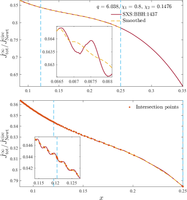
Figure 1: Intermediate steps of the cleaning procedure. The $x$-domain is separated into three different parts, delimited by the vertical lines (top panel). No smoothing is applied on the third region, while the span of the moving average changes between the first and second region. The bottom panel focuses on the intersection points between the raw function and the smoothed one, that are finally fitted with a polynomial. The inset highlights the behavior around the interface between the first and second region.

When the so-computed fluxes are depicted in terms of the gauge-invariant frequency parameter

$$x_{\rm NR}\equiv\left(\Omega_{\rm NR}\right)^{2/3}$$ (6)

one finds spurious oscillations. These oscillations are due to residual eccentricity (or other effects related to the BMS symmetry being violated Mitman et al. (2021)), and are additionally amplified when taking the derivatives. The amplification might be large and make the raw flux totally useless for any meaningful comparison with the analogous, fully nonoscillatory, EOB quantity. We have developed an efficient method to completely remove this oscillating behavior, and produce a rather clean and smooth representation of the flux versus $x$. The procedure is applied to the sample of SXS simulations reported in Table 1, that is chosen so that the datasets distribution is approximately uniform over the NR-covered portion of the parameter space. We cut each flux at the NR merger, defined as the peak of $|h_{22}|$. The procedure uses a MATLAB function called smooth, i.e. a moving average whose span can be selected by the user. The $x$-domain on which the flux function is defined is separated into three parts: the first and the second ones get smoothed with different spans, as the frequency of the oscillations progressively lowers; the third part, that is already essentially nonoscillatory, is left untouched. The three regions are optimized manually for each dataset in Table 1.

Table 1: Sample of SXS spin-aligned datasets for which we compute the angular momentum flux. From left to right the columns display: the SXS ID; the binary parameters; the highest and second-highest level of resolution; the average of the difference between the raw flux and the cleaned one.

ID	$(q,\chi_{1},\chi_{2})$	$\text{Lev}_{h}$	$\text{Lev}_{l}$	$\langle\Delta\dot{J}^{\infty}_{\rm NR-NR_{\rm clean}}\rangle$
BBH:1155	$(1,0,0)$	3	2	$1\cdot 10^{-6}$
BBH:1222	$(2,0,0)$	4	3	$5.4\cdot 10^{-5}$
BBH:1179	$(3,0,0)$	5	4	$1.8\cdot 10^{-5}$
BBH:0190	$(4.499,0,0)$	3	2	$1.5\cdot 10^{-5}$
BBH:0192	$(6.58,0,0)$	3	2	$1.3\cdot 10^{-5}$
BBH:1107	$(10,0,0)$	4	3	$7.2\cdot 10^{-5}$
BBH:1137	$(1,-0.97,-0.97)$	4	2	$6.3\cdot 10^{-5}$
BBH:2084	$(1,-0.90,0)$	4	3	$-2\cdot 10^{-6}$
BBH:2097	$(1,+0.30,0)$	4	3	$2.4\cdot 10^{-5}$
BBH:2105	$(1,+0.90,0)$	4	3	$2.3\cdot 10^{-5}$
BBH:1124	$(1,+0.99,+0.99)$	3	-	$2.6\cdot 10^{-5}$
BBH:1146	$(1.5,+0.95,+0.95)$	2	0	$1.2\cdot 10^{-5}$
BBH:2111	$(2,-0.60,+0.60)$	4	3	$-9\cdot 10^{-6}$
BBH:2124	$(2,+0.30,0)$	4	3	$9\cdot 10^{-6}$
BBH:2131	$(2,+0.85,+0.85)$	4	3	$2\cdot 10^{-5}$
BBH:2132	$(2,+0.87,0)$	4	3	$1.3\cdot 10^{-5}$
BBH:2133	$(3,-0.73,+0.85)$	4	3	$2.2\cdot 10^{-5}$
BBH:2153	$(3,+0.30,0)$	4	3	$3.6\cdot 10^{-5}$
BBH:2162	$(3,+0.60,+0.40)$	4	3	$1.7\cdot 10^{-5}$
BBH:1446	$(3.154,-0.80,+0.78)$	3	2	$9\cdot 10^{-6}$
BBH:1936	$(4,-0.80,-0.80)$	3	2	$-1.8\cdot 10^{-5}$
BBH:2040	$(4,-0.80,-0.40)$	3	2	$7\cdot 10^{-6}$
BBH:1911	$(4,0,-0.80)$	3	2	$7\cdot 10^{-6}$
BBH:2014	$(4,+0.80,+0.40)$	3	-	$-1\cdot 10^{-6}$
BBH:1434	$(4.368,+0.80,+0.80)$	3	-	$2.5\cdot 10^{-5}$
BBH:1463	$(4.978,+0.61,+0.24)$	3	2	$1.5\cdot 10^{-5}$
BBH:0208	$(5,-0.90,0)$	3	2	$9.2\cdot 10^{-5}$
BBH:1428	$(5.518,-0.80,-0.70)$	3	2	$-2\cdot 10^{-6}$
BBH:1437	$(6.038,+0.80,+0.15)$	3	2	$5\cdot 10^{-6}$
BBH:1436	$(6.281,+0.009,-0.80)$	3	2	$1\cdot 10^{-6}$
BBH:1435	$(6.588,-0.79,+0.7)$	3	2	$2\cdot 10^{-6}$
BBH:1448	$(6.944,-0.48,+0.52)$	3	-	$2.1\cdot 10^{-5}$
BBH:1375	$(8,-0.90,0)$	3	-	$2.6\cdot 10^{-5}$
BBH:1419	$(8,-0.80,-0.80)$	3	-	$-1.3\cdot 10^{-5}$
BBH:1420	$(8,-0.80,+0.80)$	3	2	$2.2\cdot 10^{-5}$
BBH:1455	$(8,-0.40,0)$	3	2	$-3\cdot 10^{-6}$

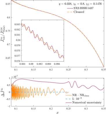
Figure 2: The cleaned numerical angular momentum flux for the simulation SXS:BBH:1437 (dashed orange) is plotted against the original one (red). The inset in the upper panel shows how the final flux follows the original curve, averaging the oscillations. In the lower panel we display the difference between the cleaned and the raw flux, whose mean (dashed light blue line) is of order $10^{-5}$, hence proving the effectiveness of the procedure. Our cleaning method also allows to estimate numerical accuracy (red curve), that is evaluated by subtracting to the cleaned flux its equivalent coming from the second-highest available resolution.

The cleaning procedure can be summarized in three steps: (i) we first apply the moving average to reduce the amplitude of the oscillations (see inset in the upper panel of Fig. 1); (ii) then we find the intersection points between the raw flux and the smoothed one, (see markers in the inset of Fig. 1); (iii) as a third step, the intersection points between the raw and the smoothed flux are fitted by a polynomial in $x$. For the datasets SXS:BBH:1155, SXS:BBH:1222, SXS:BBH:0190, SXS:BBH:0192 this is accomplished via a seventh order polynomial, while it suffices a fifth order one for the others. The outcome of the fit is finally joined to the third part that was left unmodified. The final result, after some additional smoothing at the junction point, is shown in Fig. 2. Its reliability can be verified by computing the difference with the raw data and checking that it averages zero. This is shown in the bottom panel of Fig. 2, where the residual does not show any evident global trend, actually averaging at $\sim 5\times 10^{-6}$. To obtain a conservative estimate of the NR uncertainty on the final fluxes, we apply the cleaning procedure to both the highest and second highest available resolution and then take the difference. This is also shown in the bottom panel of Fig. 2. The procedure is found to be efficient and reliable for all configurations of Table 1, where the quality of the cleaning procedure is indicated by the average of the difference between the raw flux and the cleaned one (last column of the table). The final result is displayed in Fig. 3. The figure highlights how both the value of the flux at merger and its global behavior have a clear dependence on the mass ratio and the effective Kerr parameter. This testifies how equal-mass binaries have a more adiabatic evolution, corresponding to slower plunges and a lower angular momentum loss. If the BHs have positive spins the plunge is even slower, owing to the well known effect of spin-orbit coupling (or hang-up effect) Damour (2001); Campanelli et al. (2006). Conversely for high mass ratio binaries (nearer to the test-mass limit) and negative spins, the fact that the system is progressively more and more nonadiabatic implies larger angular momentum losses, and the evolution ends at lower frequencies.

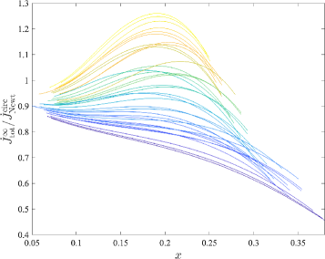
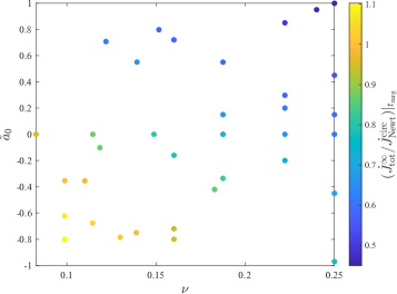
Figure 3: The top panel shows the final outcome of the Newton-normalized angular momentum flux calculation for the NR datasets of Table 1, with $x$ given by Eq. (6), shown up to merger. The color code is chosen depending on the final value of the flux, displayed in the lower panel. The merger values show a clear dependence on $\nu$ and $\tilde{a}_{0}$, mirroring whether the dynamics is more or less adiabatic: larger emissions correspond to faster plunges (with $\tilde{a}_{0}<0$).

II.2 Angular momentum flux and radiation reaction within EOB

Let us now turn to discuss EOB fluxes within TEOBResumS. To do so, we start by reviewing the analytical elements of TEOBResumS that will be useful for our discussion. We use mass-reduced phase-space variables $(r,\varphi,p_{\varphi},p_{r_{*}})$, related to the physical ones by $r=R/M$ (relative separation), $p_{r_{*}}=P_{R_{*}}/\mu$ (radial momentum), $\varphi$ (orbital phase), $p_{\varphi}=P_{\varphi}/(\mu M)$ (angular momentum) and $t=T/M$ (time). The “tortoise” radial momentum is $p_{r_{*}}\equiv(A/B)^{1/2}p_{r}$, where $A$ and $B$ are the EOB potentials (with included spin-spin interactions Damour and Nagar (2014)). The Hamilton’s equations for the relative dynamics read

$$\dot{\varphi} =\Omega=\partial_{p_{\varphi}}\hat{H}_{\rm EOB},$$ (7)

$$\dot{r} =\left(\frac{A}{B}\right)^{1/2}\partial_{p_{r_{*}}}\hat{H}_{\rm EOB},$$ (8)

$$\dot{p}_{\varphi} =\hat{{\cal F}}_{\varphi},$$

$$\dot{p}_{r_{*}} =-\left(\frac{A}{B}\right)^{1/2}\partial_{r}\hat{H}_{\rm EOB},$$ (9)

where $\hat{H}_{\rm EOB}$ is the EOB Hamiltonian Nagar et al. (2018), $\Omega$ is the orbital frequency and $\hat{{\cal F}}_{\varphi}$ is the radiation reaction force accounting for mechanical angular momentum losses due to GW emission. Note that within this context we are assuming that the radial force $\hat{{\cal F}}_{r}=0$, that is equivalent to a gauge choice for circular orbits Buonanno and Damour (2000). For a balance argument, the system angular momentum loss should be equal to the sum of the GW flux emitted at infinity, $\dot{J}_{\infty}$, and absorbed by the event horizons of the two black holes, $\dot{J}_{\rm H_{1,2}}$, that is

$$\dot{J}_{\rm system}=\hat{{\cal F}}_{\varphi}=-\dot{J}_{\infty}-\dot{J}_{\rm H_{1}}-\dot{J}_{\rm H_{2}}.$$ (10)

In general, within this equation there should be an additional term accounting for Schott contributions, that are due to the interactions between the radiation and the field. However, it is always possible to choose a gauge such that there is no Schott contribution to the angular momentum Bini and Damour (2012) and this is the choice made here (on top of neglecting $\hat{\cal{F}}_{r}$). The azimuthal radiation reaction force is hence written as

$$\hat{{\cal F}}_{\varphi}=\hat{{\cal F}}_{\varphi}^{\infty}+\hat{{\cal F}}_{\varphi}^{\rm H},$$ (11)

where $\hat{{\cal F}}_{\varphi}^{\rm H}$ is the horizon flux contribution Damour and Nagar (2014). The asymptotic term reads

$$\hat{{\cal F}}_{\varphi}^{\infty}=-\frac{32}{5}\nu r_{\omega}^{4}\Omega^{5}\hat{f}^{\infty}(v_{\varphi}^{2};\nu),$$ (12)

where $\hat{f}^{\infty}(v_{\varphi}^{2};\nu)$ is the reduced (i.e., Newton-normalized) flux function, $v_{\varphi}^{2}\equiv(r_{\omega}\Omega)^{2}$ and $r_{\omega}$ is a modified radial separation defined in such a way that $1=\Omega^{2}r_{\omega}^{3}$ is valid during the plunge, fulfilling a modified Kepler’s law that accounts for non-circularity Damour and Gopakumar (2006); Damour and Nagar (2007). The reduced flux function is defined by normalizing the resummed circularized energy flux as $\hat{f}\equiv({\cal F}_{22}^{\rm Newt})^{-1}\sum{\cal F}_{\ell m}$, with all multipoles (except $m=0$ modes) up to $\ell=8$. The Newtonian term reads ${\cal F}_{22}^{\rm Newt}=(32/5)\nu^{2}x^{5}$ and the multipolar terms ${\cal F}_{\ell m}$ are factorized and resummed analogously to what is done for the waveform Damour et al. (2013). Explicitly, building upon Ref. Damour et al. (2009), the structure of each flux multipole is

$${\cal F}_{\ell m}={\cal F}_{\ell m}^{\rm Newt}|\hat{h}_{\ell m}|^{2}{\cal F}_{\ell m}^{\rm NQC}.$$ (13)

This is related to the correction entering the factorization of the waveform multipoles

$$h_{\ell m}=h_{\ell m}^{\rm Newt}\,\hat{h}_{\ell m}\,\hat{h}_{\ell m}^{\rm NQC}$$ (14)

where $h_{\ell m}^{\rm Newt}$ is the Newtonian prefactor, $\hat{h}_{\ell m}$ is the resummed PN correction and $\hat{h}_{\ell m}^{\rm NQC}$ is the next-to-quasi-circular factor. The latter is described in more detail in Refs. Damour and Nagar (2014); Nagar et al. (2017, 2019a); Riemenschneider et al. (2021) (see in particular Sec. IIID of Nagar et al. (2019a)). For each flux mode we have

$${\cal F}_{\ell m}^{\rm NQC}=\left|\hat{h}_{\ell m}^{\rm NQC}\right|^{2}=\left(1+a_{1}^{\ell m}n_{1}^{\ell m}+a_{2}^{\ell m}n_{2}^{\ell m}\right)^{2}$$ (15)

where $(n_{1}^{\ell m},n_{2}^{\ell m})$ are functions of the radial momentum and of the radial acceleration (and a priori depend on the mode); $(a_{1}^{\ell m},a_{2}^{\ell m})$ are numerical coefficients that are informed by NR simulations Damour and Nagar (2014); Nagar et al. (2017) via an iterative procedure Damour and Nagar (2009). NQC corrections can, and actually should, be applied to each waveform (and thus flux) mode since they complete the analytical waveform, that is quasicircular by construction. In practice, within TEOBResumS we add NQC corrections only in the $(2,2)$ flux mode, while the waveform is NQC-completed up to $\ell=m=5$ Nagar et al. (2019a).

Finally, we remind that TEOBResumS is NR-informed via two different parameters, $a_{6}^{c}(\nu)$ and $c_{3}(\nu,\tilde{a}_{1},\tilde{a}_{2})$, respectively tuning the $A$ potential and the spin-orbit sector of the model. Details on these functions can be found in Sec. IIC of Ref. Nagar et al. (2020).

For most of the analyses carried out in the following, we make use of the private MATLAB version of TEOBResumS, in which we implement the changes for TEOBResumS_NQC_lm. The publicly available $C$ version is used in the unfaithfulness calculation for the standard TEOBResumS.

II.3 Comparing NR and EOB fluxes

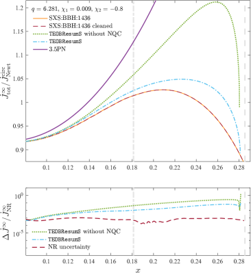
Figure 4: Comparing Newton normalized total angular momentum fluxes summed up to $\ell_{\rm max}=8$. The upper panel shows: (i) the raw numerical flux (orange) and as its cleaned version (dashed red); (ii) the EOB flux with $\ell=m=2$ NQC corrections (dash-dotted light blue) and without (dotted green); (iii) the 3.5PN flux (purple). From left to right, the vertical lines indicate the EOB LSO and the NR merger respectively. Fractional differences are shown in the bottom panel, together with the NR uncertainty. NQC corrections are essential to reduce the gap between the EOB and NR curves.

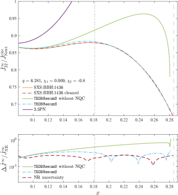
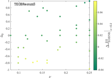
Figure 5: Top: Comparing Newton-normalized $\ell=m=2$ angular momentum fluxes, including again NR, the EOB fluxes with and without NQC corrections, and the 3.5PN result. Remarkably, the fractional difference with NR for the NQC-corrected EOB curve is of order $10^{-3}$ up to merger. The vertical lines indicate the LSO and the merger point. The $\ell=m=2$ numerical flux has been cleaned separately from the total one, and the difference between the raw flux and the final fit averages to $-2\cdot 10^{-5}$. Bottom: Fractional differences for the EOB/NR $\ell=m=2$ fluxes at $x=0.2$ for all configurations of Table 1. The largest differences occur when $\tilde{a}_{0}<0$, where $x=0.2$ approximately corresponds to the plunge regime.

Let us now move to compare EOB and NR fluxes. The Newton-normalized EOB flux is expressed versus $x_{\rm EOB}=\Omega^{2/3}$, while the NR curve is expressed versus $x_{\rm NR}=\Omega_{\rm NR}^{2/3}$ as defined above. To simplify the notation, in the figure we will simply use $x$ for the horizontal axis, but it is intended that $x=x_{\rm NR}$ when dealing with the NR curve and $x=x_{\rm EOB}$ for the EOB curve. As an illustrative configuration we choose SXS:BBH:1436, corresponding to parameters $(q,\chi_{1},\chi_{2})=(6.281,0.009,-0.8)$. The Newton-normalized, total, angular momentum flux, summed up to $\ell_{\rm max}=8$ is displayed in Fig. 4. In particular, the figure shows: (i) the raw and cleaned NR fluxes, that are effectively indistinguishable on this scale; (ii) two EOB fluxes, one with the $\ell=m=2$ NQC correction in the flux and another without it; (iii) the 3.5PN flux. The EOB fluxes prove both the power of resummation techniques and the effectiveness of NQC corrections in achieving a good agreement with the NR quantities. The upper panel in Figure 5 is analogous to Fig. 4, but only focuses on the $\ell=m=2$ contribution. The most interesting fact inferred by the plot is that the NQC factor is crucial to yield a fractional difference $\sim 10^{-3}$ up to merger. The lower panel of the same figure shows the distribution of the EOB/NR fractional difference at $x=0.2$ over the parameter space. This seems to point out to a decreased agreement for configurations having a negative $\tilde{a}_{0}$, but one has to note however that, as can be seen in Fig. 3, the fluxes for these datasets end at lower frequencies and hence $x=0.2$ corresponds to the late plunge.

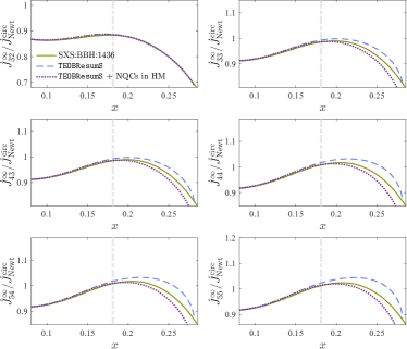
Figure 6: Exploring the importance of higher modes using the SXS:BBH:1436 dataset. In each panel the flux is summed up to the indicated $(\ell,m)$ mode. NQC corrections are included either in the $\ell=m=2$ EOB mode only (dashed blue line) or in all $\ell=m$ modes up to $\ell=5$ (dotted purple line). The NR-informed NQC corrections in higher modes are essential to improve the EOB/NR agreement beyond plunge (the vertical line indicates the LSO frequency) and up to merger.

Table 2: Binary configurations, first-guess values of $c_{3}$ used to inform the global interpolating fit given in Eq. (III), and the corresponding $c_{3}^{\rm fit}$ values.

$\#$	ID	$(q,\chi_{1},\chi_{2})$	$\tilde{a}_{0}$	$c_{3}^{\rm first\;guess}$	$c_{3}^{\rm fit}$
1	BBH:1137	$(1,-0.97,-0.97)$	$-0.97$	89.7	89.33
2	BBH:0156	$(1,-0.9498,-0.9498)$	$-0.95$	88.5	88.33
3	BBH:0159	$(1,-0.90,-0.90)$	$-0.90$	84.5	85.86
4	BBH:2086	$(1,-0.80,-0.80)$	$-0.80$	82	80.93
5	BBH:2089	$(1,-0.60,-0.60)$	$-0.60$	71	71.19
6	BBH:0150	$(1,+0.20,+0.20)$	$+0.20$	35.5	35.73
7	BBH:2102	$(1,+0.60,+0.60)$	$+0.60$	22.2	21.67
8	BBH:2104	$(1,+0.80,+0.80)$	$+0.80$	15.9	16.31
9	BBH:0153	$(1,+0.85,+0.85)$	$+0.85$	15.05	15.29
10	BBH:0160	$(1,+0.90,+0.90)$	$+0.90$	14.7	14.5
11	BBH:0157	$(1,+0.95,+0.95)$	$+0.95$	14.3	14.1
12	BBH:0177	$(1,+0.99,+0.99)$	$+0.99$	14.2	14.29
13	BBH:0004	$(1,-0.50,0.0)$	$-0.25$	55.5	54.44
14	BBH:0005	$(1,+0.50,0.0)$	$+0.25$	35	34.17
15	BBH:2105	$(1,+0.90,0.0)$	$+0.45$	27.7	27.21
16	BBH:2106	$(1,+0.90,+0.50)$	$+0.70$	19.1	19.09
17	BBH:0016	$(1.5,-0.50,0.0)$	$-0.30$	56.2	56.14
18	BBH:1146	$(1.5,+0.95,+0.95)$	$+0.95$	14.35	13.98
19	BBH:2129	$(2,+0.60,0.0)$	$+0.40$	29.5	29.31
20	BBH:2130	$(2,+0.60,+0.60)$	$+0.60$	23	22.41
21	BBH:2131	$(2,+0.85,+0.85)$	$+0.85$	16.2	15.73
22	BBH:2139	$(3,-0.50,-0.50)$	$-0.50$	65.3	62.45
23	BBH:0036	$(3,-0.50,0.0)$	$-0.38$	58.3	57.62
24	BBH:0174	$(3,+0.50,0.0)$	$+0.37$	28.5	30.87
25	BBH:2158	$(3,+0.50,+0.50)$	$+0.50$	27.1	26.64
26	BBH:2163	$(3,+0.60,+0.60)$	$+0.60$	24.3	23.56
27	BBH:0293	$(3,+0.85,+0.85)$	$+0.85$	17.1	17.05
28	BBH:1447	$(3.16,+0.7398,+0.80)$	$+0.75$	19.2	19.46
29	BBH:2014	$(4,+0.80,+0.40)$	$+0.72$	21.5	21.52
30	BBH:1434	$(4.37,+0.7977,+0.7959)$	$+0.80$	19.8	20.05
31	BBH:0111	$(5,-0.50,0.0)$	$-0.42$	54	57.18
32	BBH:0110	$(5,+0.50,0.0)$	$+0.42$	32	30.98
33	BBH:1432	$(5.84,+0.6577,+0.793)$	$+0.68$	25	24.42
34	BBH:1375	$(8,-0.90,0.0)$	$-0.80$	64.5	65.12
35	BBH:0114	$(8,-0.50,0.0)$	$-0.44$	57	56.07
36	BBH:0065	$(8,+0.50,0.0)$	$+0.44$	29.5	31.78
37	BBH:1426	$(8,+0.4838,+0.7484)$	$+0.51$	30.3	29.98

The cumulative importance of higher modes with respect to the $\ell=m=2$ one is studied in Fig. 6 for the same SXS:BBH:1436 configuration. The figure contrasts the EOB flux with the NR one, where both functions incorporate modes summed up to the indicated $(\ell,m)$ value. The plot shows that for the standard TEOBResumS the EOB/NR agreement progressively worsens during the late inspiral up to merger, due to the lack of the NR-informed NQC corrections beyond the $\ell=m=2$ ones. Including NQC corrections in the flux in all the $\ell=m$ modes up to $\ell=5$ yields a closer agreement between the analytical and numerical fluxes up to merger. The NQC parameters are determined with the usual iteration procedure, although we maintain the same values of the NR-informed parameters $(a_{6}^{5},c_{3})$ determined with the standard $\ell=m=2$ NQC correction. The effect is very evident for this specific dataset, but it is a feature that is always present, also for other configurations. This exercise indicates that to increase the physical completeness and NR-consistency of TEOBResumS it would be needed to include NQC corrections at least in the $\ell=m$ multipoles in the flux. Evidently, this operation will eventually imply the need of constructing new NR-informed $(a_{6}^{c},c_{3})$ functions that are consistent with the new choice of radiation reaction.

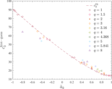
Figure 7: The first-guess $c_{3}$ values of Table 2 versus the spin variable $\tilde{a}_{0}$. The unequal-spin and unequal-mass points can be essentially seen as a correction to the equal-mass, equal-spin values. The latter are fitted to obtain the first part of the fit, $c_{3}^{\rm eq}$ (dashed red).

III Improving the consistency between waveform and flux of TEOBResumS

Let us construct a modified TEOBResumS model that incorporates iterated NQC corrections in all $\ell=m$ modes in the flux up to $\ell=5$. Since we are modifying the radiation reaction, this choice in principle calls for a new determination of both the $a_{6}^{c}$ and $c_{3}$ functions. However, we have verified that the improvements brought by a newly tuned $a_{6}^{c}(\nu)$ are marginal, so that, for the sake of simplicity, we keep its standard expression that we quote here for completeness as

$$a_{6}^{c}=n_{0}\dfrac{1+n_{1}\nu+n_{2}\nu^{2}+n_{3}\nu^{3}}{1+d_{1}\nu},$$ (16)

where

$$n_{0} =\;\;\;5.9951,$$ (17)

$$n_{1} =-34.4844,$$ (18)

$$n_{2} =-79.2997,$$ (19)

$$n_{3} =\;\;\;713.4451,$$ (20)

$$d_{1} =-3.167.$$ (21)

By contrast, we look for a new NR-informed representation of $c_{3}$. We follow our usual procedure, that is described for example in Sec. IIB.2 of Ref. Nagar et al. (2018). Typically, for each NR dataset one determines a value of $c_{3}$ so that the EOB/NR accumulated phase difference up to merger is within (or compatible with) the NR phase uncertainty at NR merger. This leaves a certain flexibility and arbitrariness in the choice of $c_{3}$ and, in previous attempts, we were typically accepting EOB/NR phase differences of the order of 0.1-0.2 rad at merger. Here, on the understanding that the NR phase uncertainty might be overestimated by taking the difference between the two highest resolutions, we attempt to ask more, requiring that the EOB/NR phase difference is as flat as possible through inspiral, merger and ringdown when the two waveforms are aligned during the early inspiral. As a cross check, we also align the two waveforms during the late plunge, just before merger, to verify that the phase difference keeps remaining flat. This further proves that the $c_{3}$ determination, that mostly affects the plunge phase, is done robustly. To exploit at best current NR information, we consider a sample of 37 SXS configurations, most of which were already taken into account in the previous determinations of $c_{3}$. Here we replaced some datasets used in Ref. Nagar et al. (2018) with newer ones with improved accuracy and included a few more simulations so as to cover the parameter space more efficiently. Table 2 reports the SXS configurations, the corresponding values of $\tilde{a}_{0}$ , the first-guess values of $c_{3}$ obtained with the procedure explained above as well as the corresponding ones obtained after a global fit. Specifically, the $c_{3}^{\rm first-guess}$ data of Table 2 are fitted with a global function as $c_{3}(\nu,\tilde{a}_{0},\tilde{a}_{12})$ that reads

$$c_{3}(\nu,\tilde{a}_{0},\tilde{a}_{12})=\, p_{0}\dfrac{1+n_{1}\tilde{a}_{0}+n_{2}\tilde{a}_{0}^{2}+n_{3}\tilde{a}_{0}^{3}+n_{4}\tilde{a}_{0}^{4}}{1+d_{1}\tilde{a}_{0}}$$

$$+ p_{1}\tilde{a}_{0}\sqrt{1-4\nu}+p_{2}\tilde{a}_{0}^{2}\sqrt{1-4\nu}$$

$$+ p_{3}\tilde{a}_{0}\nu\sqrt{1-4\nu}+p_{4}\tilde{a}_{12}\nu^{2},$$ (22)

where the fitted parameters are

$$p_{0} =\;\;\;43.872788,$$ (23)

$$n_{1} =-1.849495,$$ (24)

$$n_{2} =\;\;\;1.011208,$$ (25)

$$n_{3} =-0.086453,$$ (26)

$$n_{4} =-0.038378,$$ (27)

$$d_{1} =-0.888154,$$ (28)

$$p_{1} =\;\;\;26.553,$$ (29)

$$p_{2} =-8.65836,$$ (30)

$$p_{3} =-84.7473,$$ (31)

$$p_{4} =\;\;\;24.0418\ .$$ (32)

Figure 7 highlights that the span of the “best” (first-guess) values of $c_{3}$ is rather limited (especially for spins aligned with the orbital angular momentum) around the equal-mass, equal-spin case. As in previous work, the fitting procedure consists of two steps. First, one fits the equal-mass, equal-spin data with a quasi-linear function of $\tilde{a}_{0}=\tilde{a}_{1}+\tilde{a}_{2}$ with $\tilde{a}_{1}=\tilde{a}_{2}$. This delivers the six parameters $(p_{0},n_{1},n_{2},n_{3},n_{4},d_{1})$. The corresponding fit $c_{3}^{\rm eq}$ is shown as a dashed red curve in Fig. 7. Note that the analytical structure of the fitting function was chosen in order to accurately capture the nonlinear behavior of $c_{3}$ for $\tilde{a}_{0}\to 1$. In the second step one subtracts this fit from the corresponding $c_{3}^{\rm first-guess}$ values and fits the residual. This determines the parameters $(p_{1},p_{2},p_{3},p_{4})$. The novelty with respect to previous work is that the functional form chosen for the unequal-mass, unequal-spin fit is more effective in capturing the first-guess values all over the SXS sample considered.

To give a flavor of the improved EOB/NR agreement that can be obtained with the new $c_{3}$ and with the new radiation reaction, let us report a few examples. From now on we will refer to the improved model as TEOBResumS_NQC_lm, to easily distinguish it from TEOBResumS. Figure 8 shows the updated flux comparison for SXS:BBH:1436, and also includes the dataset SXS:BBH:1437 with $(q,\chi_{1},\chi_{2})=(6.038,0.8,0.1476)$. The addition of NQC corrections to $\ell=m$ modes up to $\ell=5$ of the radiation reaction is essential to improve the behavior of the analytic flux towards merger. For TEOBResumS_NQC_lm the fractional difference between EOB/NR total fluxes for the configuration SXS:BBH:1436 remains below $10^{-2}$ until $x\sim 0.26$. By contrast, in Fig. 4, the fractional difference for TEOBResumS already reached $10^{-2}$ at the LSO and kept growing until merger.

We finally test the performance of the model over all datasets of Table 1, by computing the fractional difference between EOB and NR (total) fluxes at $x=0.2$ for both TEOBResumS and TEOBResumS_NQC_lm, as shown respectively in the top and bottom panel of Fig. 9. Here one can see an evident improvement for larger mass ratios and negative values of the effective Kerr parameter.

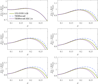
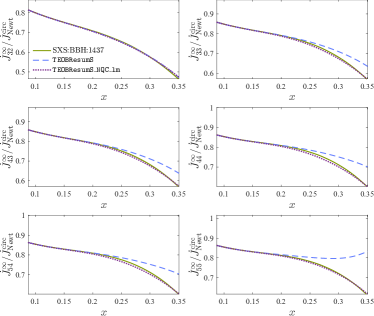
Figure 8: Left: Analogous of Fig. 6 obtained using the new model, showing that the change in $c_{3}$ does not affect the behavior of the flux. When summing up to $\ell=8$ as done in Fig. 4, the EOB/NR fractional difference for TEOBResumS_NQC_lm remains below $10^{-2}$ for most of the evolution, even beyond the LSO. Right: Contrasting the performance of TEOBResumS and TEOBResumS_NQC_lm for the dataset SXS:BBH:1437 with $(q,\chi_{1},\chi_{2})=(6.038,0.8,0.1476)$. The behavior of the flux up to $\ell=8$ progressively gets less robust and is discussed in Appendix A.

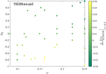
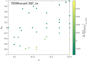
Figure 9: Fractional EOB/NR flux differences at $x=0.2$ for TEOBResumS (top) and TEOBResumS_NQC_lm (bottom) evaluated for the sample of SXS data of Table 1. For TEOBResumS_NQC_lm we are excluding from the points two configurations, corresponding to datasets SXS:BBH:1419 and SXS:BBH:1375, where the contribution of modes with $\ell_{\rm max}>5$ becomes important towards merger. These will be discussed in Appendix A.

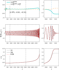
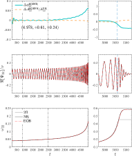
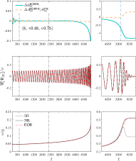
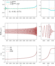
Figure 10: EOB/NR time-domain phasing for two illustrative datasets: SXS:BBH:1463 with $(q,\chi_{1},\chi_{2})=(4.978,+0.61,+0.24)$ (top panels) and SXS:BBH:1426 with $(q,\chi_{1},\chi_{2})=(8,+0.48,+0.75)$ (bottom panels), using TEOBResumS (left) and TEOBResumS_NQC_lm (right). Each plot shows: (i) the phase difference and the relative amplitude difference; (ii) the real parts of the EOB and NR waveforms; (iii) the instantaneous GW frequency together with twice the orbital frequency $\Omega$. Vertical dash-dotted lines indicate the alignment interval. The phase differences $\Delta\phi^{\rm EOBNR}_{22}$ at merger (vertical dashed blue line) are respectively $(-0.34,-0.70)$ rad for TEOBResumS and become $(-0.14,-0.11)$ for TEOBResumS_NQC_lm. Note that only SXS:BBH:1426 was used to inform $c_{3}$.

Another example is shown in Fig. 10, that focuses on time-domain phasings. We use here the Regge-Wheeler-Zerilli normalized waveform, defined as $\Psi_{\ell m}=h_{\ell m}/\sqrt{(\ell-1)\ell(\ell+1)(\ell+2)}$. The EOB waveforms have been obtained by setting the spin values with 6 digits precision, considering the initial $\chi_{1},\chi_{2}$ given in the metadata file for each simulation. The figure contrasts EOB/NR waveform phasings for the $\ell=m=2$ multipole, considering datasets SXS:BBH:1463 (first row) and SXS:BBH:1426 (second row) using TEOBResumS (left) and TEOBResumS_NQC_lm (right). As usually done, in this case we are using $N=3$ extrapolation order for the SXS waveforms. In each figure, the top panels show the phase and amplitude difference, where $\Delta\phi^{\rm EOBNR}_{22}\equiv\phi^{\rm EOB}_{22}-\phi^{\rm NR}_{22}$. The EOB/NR phasing agreement is better for TEOBResumS_NQC_lm than for TEOBResumS, although the SXS:BBH:1426 dataset is among those used to inform the new expression of $c_{3}$.

IV EOB/NR $\ell=m=2$ unfaithfulness

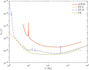
Figure 11: Sensitivity curves for the three detectors we take into consideration in computing the unfaithfulness for the two versions of our model: Advanced LIGO, Einstein Telescope (ET) and Cosmic Explorer (CE). Here ET-C is the sensitivity model described in Ref. Hild et al. (2010), while ET-D is the latest version Hild et al. (2011).

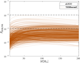
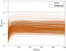
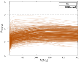
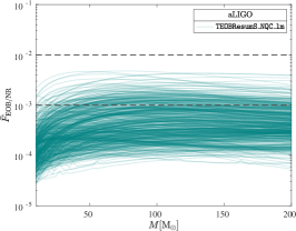
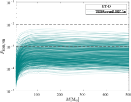
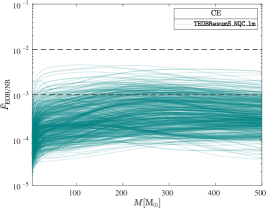
Figure 12: EOB/NR unfaithfulness for TEOBResumS (top panels) and TEOBResumS_NQC_lm (bottom panels) evaluated over the sample of 534 nonprecessing quasicircular datasets of the SXS catalog already considered in Ref. Riemenschneider et al. (2021), using: (i) the zero-detuned, high-power noise spectral density of Advanced LIGO (first column), (ii) the latest version of the expected noise for the Einstein Telescope (second column), (iii) the expected noise for Cosmic Explorer (third column). We observe here how the changes implemented in the new version of our model ensure a slight decrease in $\bar{F}_{\rm EOB/NR}$, whose average is between $10^{-3}$ and $10^{-4}$.

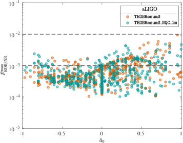
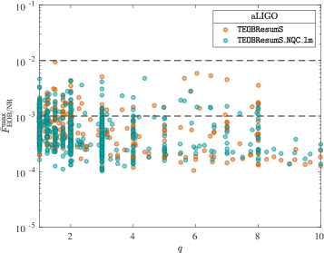
Figure 13: Contrasting $\bar{F}^{\rm max}_{\rm EOB/NR}$ for TEOBResumS and TEOBResumS_NQC_lm versus $\tilde{a}_{0}$ and $q$, using the PSD of Advanced LIGO. This complements the top panels of Fig. 12.

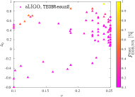
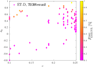
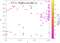
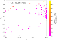
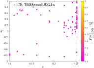
Figure 14: Distribution over the parameter space $(\nu,\tilde{a}_{0})$ of those configurations whose $\bar{F}^{\rm max}_{\rm EOB/NR}$ exceeds $10^{-3}$, for aLIGO (first row), ET-D (second row), CE (third row), both for TEOBResumS (left column) and its updated version (right column). Notably, the changes implemented in TEOBResumS_NQC_lm lower the maximum unfaithfulness, although we see that higher values of the spin remain the most challenging ones to be modeled, along with the comparable-mass case.

A global view of the EOB/NR agreement is given by the computation of the EOB/NR unfaithfulness as a function of the total mass of the system. As done for the time-domain phasing, for the EOB spin values we take the initial $(\chi_{1},\chi_{2})$ given in the metadata file for each simulation with 6 digits precision. For simplicity, here we focus only on the $\ell=m=2$ mode. Considering two waveforms $(h_{1},h_{2})$ with same fixed mass ratio and spins, the unfaithfulness is a function of the total mass $M$ of the binary and is defined as

$$\bar{F}(M)\equiv 1-F=1-\max_{t_{0},\phi_{0}}\dfrac{\langle h_{1},h_{2}\rangle}{||h_{1}||||h_{2}||},$$ (33)

where $(t_{0},\phi_{0})$ are the initial time and phase, $||h||\equiv\sqrt{\langle h,h\rangle}$, and the inner product between two waveforms is defined as $\langle h_{1},h_{2}\rangle\equiv 4\Re\int_{f_{\rm min}^{\rm NR}(M)}^{\infty}\tilde{h}_{1}(f)\tilde{h}_{2}^{*}(f)/S_{n}(f)\,df$, where $\tilde{h}(f)$ denotes the Fourier transform of $h(t)$, $S_{n}(f)$ is the detector’s power spectral density (PSD) and $f_{\rm min}^{\rm NR}(M)=\hat{f}^{\rm NR}_{\rm min}/M$ is the initial frequency of the NR waveform. In practice, the integral is done up to a maximal NR frequency $f_{\rm max}^{\rm NR}$ that is chosen as the frequency where the amplitude of $\tilde{h}_{\rm NR}$ is $10^{-3}$. Waveforms are tapered in the time-domain at the beginning of the inspiral so as to reduce the presence of high-frequency oscillations in the corresponding Fourier transforms. As a step forward to previous work, we here consider for this calculation not only the standard zero-detuned, high-power noise spectral density of Advanced LIGO aLI , but also the anticipated PSD of Einstein Telescope, considering its latest sensitivity model ET-D Hild et al. (2011), and of Cosmic Explorer Evans et al. (2021). The corresponding PSDs are shown in Fig. 11, together with the less recent ET-C version of the PSD of Einstein Telescope Hild et al. (2010). As a complementary analysis we perform the unfaithfulness computation for this PSD in Appendix C.

The outcome of the $\bar{F}(M)$ computation is shown in Fig. 12, where we used Eq. (33) with $h_{1}=h_{\rm EOB}$ and $h_{2}=h_{\rm NR}$. For each detector choice, the top panels of the figure displays the results obtained with TEOBResumS, while the bottom ones those pertaining to TEOBResumS_NQC_lm. For what concerns the aLIGO PSD, the first column of Fig. 12 highlights that $\bar{F}^{\rm max}_{\rm EOB/NR}$ comfortably stays well below the $10^{-2}$ threshold, all over the parameter space. More precisely, one finds that for TEOBResumS_NQC_lm the datasets in the range $10^{-3}<\bar{F}^{\rm max}_{\rm EOB/NR}<10^{-2}$ are 18.4% (see Table 3), out of which 1.7% have a maximum $\bar{F}_{\rm EOB/NR}$ value above $3\times 10^{-3}$, where the latter percentage value is lower than the one related to TEOBResumS. The largest unfaithfulness values obtained with TEOBResumS_NQC_lm, $\bar{F}^{\rm max}_{\rm EOB/NR}=(0.47,0.49)\%$, correspond respectively to the extremely spinning configuration SXS:BBH:1124 with $(1,+0.998,+0.998)$ and to the configuration SXS:BBH:1434 with $(4.367,+0.798,+0.795)$. In general, as deducible from Fig. 14, the largest values of $\bar{F}^{\rm max}_{\rm EOB/NR}$ are obtained for the datasets with individual spins large and positive, i.e. in a regime where we a priori expect the largest uncertainties in both the NR waveforms and in the model. Our result already represents nonnegligible quantitative progress with respect to Refs. Nagar et al. (2020); Riemenschneider et al. (2021). Still, there exists room for improvement, since the NR error is estimated between $10^{-6}$ and $10^{-4}$, as shown in the right panel of Fig. 2 of Ref. Nagar et al. (2020).

For what concerns ET-D, the second column of Fig. 12 and Table 3 highlight that $\bar{F}^{\rm max}_{\rm EOB/NR}$ mostly stays below $10^{-3}$. For TEOBResumS_NQC_lm, there are only 11 configurations with $\bar{F}^{\rm max}_{\rm EOB/NR}>3\times 10^{-3}$, and again the highest values correspond to SXS:BBH:1124 and SXS:BBH:1434. Moreover, 79.9% of the total number of mismatches for TEOBResumS_NQC_lm are in the range $10^{-4}<\bar{F}_{\rm EOB/NR}<10^{-3}$ and 3.9% of the total mismatches are below $10^{-4}$ (see Table 3).

Finally, regarding CE, only 1.3% of the configurations have $\bar{F}^{\rm max}_{\rm EOB/NR}>3\cdot 10^{-3}$, and the percentage of those below $10^{-3}$ reaches 84.1%. It is quite remarkable that for this detector $6.4\%$ of the total mismatches using TEOBResumS_NQC_lm are below $10^{-4}$.

Table 3: Quantifying the EOB/NR agreement. The central columns of the table contain the fraction of datasets whose maximum unfaithfulness $\bar{F}^{\rm max}_{\rm EOB/NR}$ is within the indicated limits for either TEOBResumS or TEOBResumS_NQC_lm. The last two columns display percentage numbers out of all the mismatch values. These are found independently of the single simulations, by considering how many points pertaining to the curves of Fig. 12 fall into a certain range of $\bar{F}$. The range in $M$ is $2.5M_{\odot}$.

		$\bar{F}^{\rm max}<10^{-3}$	$10^{-3}<\bar{F}^{\rm max}<10^{-2}$	$\bar{F}^{\rm max}>3\times 10^{-3}$	$10^{-4}<\bar{F}<10^{-3}$	$\bar{F}<10^{-4}$
aLIGO	TEOBResumS	83.1%	16.9%	2.1%	83.9%	3.1%
	TEOBResumS_NQC_lm	82.0%	18.4%	1.7%	81.5%	3.8%
ET-D	TEOBResumS	83.5%	15.9%	2.6%	82.9%	3.2%
	TEOBResumS_NQC_lm	81.5%	18.5%	2.1%	79.9%	3.9%
CE	TEOBResumS	85.6%	14.8%	1.7%	84.7%	5.2%
	TEOBResumS_NQC_lm	84.1%	16.7%	1.3%	82.8%	6.4%

Concerning the two configurations displayed in Fig. 10, the lowered phase difference at merger for TEOBResumS_NQC_lm reflects in a slightly lower value of $\bar{F}^{\rm max}_{\rm EOB/NR}$. Namely, for the dataset SXS:BBH:1463, the [%] unfaithfulness switches from $(0.1437,0.1736,0.1323)$ respectively for aLIGO, ET-D and CE to $(0.1434,0.1703,0.1323)$, while for the dataset SXS:BBH:1426, the values lower from $(0.1671,0.1985,0.1546)$ to $(0.0675,0.0731,0.0613)$.

Figures 12, 13 and 14 represent, to our knowledge, the first systematic assessment of the quality of a state-of-the-art waveform model in view of the 3G detector effort Reitze et al. (2021); Couvares et al. (2021); Punturo et al. (2021); Katsanevas et al. (2021); Kalogera et al. (2021); McClelland et al. (2021). Our plots look a bit more optimistic than the conclusions of Ref. Pürrer and Haster (2020), that assessed the quality of the phenomenological waveform model IMRPhenomPv2 for specific configurations, and concluded that the accuracy of current waveform models needs to be improved by at least three orders of magnitude. If this is certainly true of IMRPhenomPv2, it doesn’t seem to be the case for the spin-aligned model that we are discussing here, as it already grazes the expected detector calibration uncertainty, $\sim 10^{-5}$, for masses up to $20M_{\odot}$. For larger values of $M$, where the detector is mostly sensitive to the ringdown, $\bar{F}_{\rm EOB/NR}$ goes up to $10^{-3}$ for several configurations. This however should be carefully interpreted, since it is related to two physical facts: (i) on the one hand, the quality of the late part of the NR ringdown might be more or less noisy depending on the configuration, thus affecting the unfaithfulness calculation; (ii) on the other hand, even if there was no relevant numerical noise, there are differences between the EOB modeled ringdown and the actual one. In particular, the absence of mode mixing between positive and negative frequency QNMs (a phenomenon that is present especially for spins anti-aligned with the angular momentum) can play a role in this context. In addition, one should also be aware of the fact that the NR-informed postmerger was constructed using SXS data extrapolated with $N=2$ Nagar et al. (2020), since this reduces the amount of NR noise during this specific part of the waveform. However, the EOB/NR comparison is done using $(N=3)$-extrapolated waveform data, that gives a good compromise between the inspiral and the merger-ringdown part of the signal. This means that the differences that we see in Fig. 12 for large masses are partly coming from the NR simulations and not from the model. We thus expect that our EOB/NR comparisons will benefit of improved NR simulations that use Cauchy Characteristic Extraction Moxon et al. (2021); Fischer et al. (2021); Zertuche et al. (2021).

On a more general ground, a precise assessment of the accuracy of the current version(s) of TEOBResumS for ET will require dedicated injection/recovery campaigns. Nonetheless our analysis seems to indicate that both versions of TEOBResumS, either the standard or the NQC-improved one, already offer a reliable starting point to investigate PE having in mind 3G detectors. To obtain such result it was crucial to improve the self-consistency of the model and to provide a new analytical representation of the $c_{3}$ function carefully selecting a new sample of useful NR datasets.

V Contrasting TEOBResumS and SEOBNRv4HM waveform models

Now that we have explored the performance of TEOBResumS under a different point of view and shown how to improve it further, let us shift to compare it with SEOBNRv4HM Bohé et al. (2017); Cotesta et al. (2020); Ossokine et al. (2020). This model is another state-of-the-art EOB model informed by NR simulations and differs from TEOBResumS for several structural choices, that involve the structure of the Hamiltonian, the gauge, the analytic content and the resummation strategies. A comprehensive analysis of what distinguishes the Hamiltonians of TEOBResumS and of SEOBNRv4HM is presented in Ref. Rettegno et al. (2019). The SEOBNRv4 model was presented in 2016 and never structurally updated since, except for the addition of higher modes Cotesta et al. (2020), without any change to the dynamics, and precession Ossokine et al. (2020). The purpose of this section is to discuss more specific comparisons between the two models, especially focusing on frequencies and angular momentum fluxes. Moreover, even if TEOBResumS has been publicly available for many years Nagar et al. (2018), direct comparisons involving both EOB models and the full NR catalog do not seem to exist in the literature. Note however that SEOBNRv4HM was compared to the most recent generation of phenomenological models (see in particular Fig.17 of Ref. Pratten et al. (2020)). We aim at filling this gap by providing one-to-one comparisons between SEOBNRv4HM and TEOBResumS that involve the important observables discussed so far: (i) angular momentum fluxes; (ii) waveform amplitude and frequency and the consistency of this latter with the dynamics; (iii) EOB/NR unfaithfulness computations taking into account also 3G detectors. In this section we will use only the standard version of TEOBResumS. In addition, for the unfaithfulness calculation we will use the publicly available $C$ implementation, that employs fits for the $\ell=m=2$ NQC parameters entering the flux as well as the (iterated) post-adiabatic approximation Nagar and Rettegno (2019) to efficiently describe the inspiral, as detailed in Ref. Riemenschneider et al. (2021).

V.1 Angular momentum fluxes

Let us firstly discuss the flux of angular momentum. To begin with, one has to be aware that – to the best of our knowledge – the dynamical phase-space variables are not among the standard outputs of the SEOBNRv4HM implementation within LALSimulation, so that some modifications of the code are needed. This was done and explicitly described already in Ref. Nagar et al. (2019a). The simplest way to compute the angular momentum flux for SEOBNRv4HM is by taking the time derivative of the angular momentum $p_{\varphi}$, i.e. using the relation

$$\dot{J}_{\tt SEOB}=-\dot{p}_{\varphi}^{\tt SEOB}=-\hat{\cal F}_{\varphi}^{\tt SEOB}.$$ (34)

Figure 15 displays the related fluxes for the configurations $(1.5,0.95,0.95)$, $(2,0.85,0.85)$, $(2,-0.6,0.6)$ and $(5.52,-0.8,-0.7)$, corresponding to SXS datasets SXS:BBH:1146, SXS:BBH:2131, SXS:BBH:2111 and SXS:BBH:1428. Each panel compares five curves: (i) the NR flux (red); (ii) the standard TEOBResumS flux; (iii) the flux from TEOBResumS without the $\ell=m=2$ NQC corrections; (iv) the SEOBNRv4HM flux. Let us firstly focus on the two cases with the largest spins, top row of Fig. 15: the figure highlights the differences between the SEOBNRv4HM and NR fluxes. We believe this is related to the SEOBNRv4HM dynamics for these two configurations, as we will further point out in Sec. V.2 below. By contrast, the TEOBResumS fluxes look consistent with the NR one. In particular, the agreement that can be reached between TEOBResumS and NR without the NQC correction factor is remarkable. However, this also shows that the NQC implementation should be revised for large spins, since it introduces nonnegligible differences already during the inspiral (see also Appendix A).

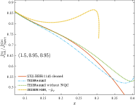
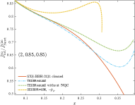
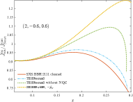
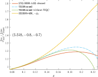
Figure 15: For the configurations corresponding to simulations SXS:BBH:1146, SXS:BBH:2131, SXS:BBH:2111, SXS:BBH:1428 we show several angular momentum fluxes: (i) the NR one (orange), (ii) the TEOBResumS one (dash-dotted light blue), (iii) the TEOBResumS one without the NQC correction in the $\ell=m=2$ mode (dash-dotted green), (iii) the corresponding flux from SEOBNRv4HM computed as $-\dot{p}_{\varphi}$ (dotted yellow).

The differences between the SEOBNRv4HM and NR fluxes remain large also in the other two cases (bottom row of Fig. 15). Given the many structural differences between the SEOBNRv4HM and TEOBResumS models, it is difficult to precisely track what are the elements within SEOBNRv4HM that are responsible of the flux behavior. The lack of the NQC factor in the SEOBNRv4HM flux is seemingly not enough to explain the differences that appear in the bottom panels of Fig. 15, since the SEOBNRv4HM curve differs even from the NQC-free flux of TEOBResumS. Let us mention at least two other differences that may be relevant in strong field. First of all, although the SEOBNRv4HM flux shares the same formal functional form of the TEOBResumS one, the definition of $r_{\omega}$ is different (see e.g. Cotesta et al. (2018)). In addition, the PN truncation and the resummation of each waveform multipole, including the quadrupole one, differs between one model and the other.

V.2 Waveform amplitude and frequency

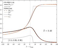
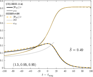
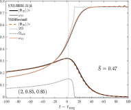
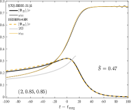
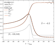
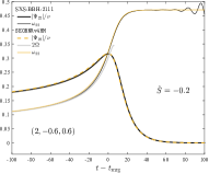
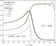
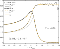
Figure 16: Contrasting TEOBResumS (left) and SEOBNRv4HM (right). For each configuration we show: (i) the waveform amplitude, (ii) the instantaneous gravitational wave frequency, (iii) twice the orbital frequency $\Omega$ and (iv) the pure orbital frequency $\Omega_{\rm orb}$ (i.e., without the spin-orbit contribution). Each binary is also labeled by its effective spin $\hat{S}\equiv(S_{1}+S_{2})/M^{2}$. For any configuration TEOBResumS maintains an excellent consistency between (twice) the orbital frequency and the gravitational wave frequency. This is especially true, as a priori expected, in the highly adiabatic cases with large positive spins where NQC corrections have a very limited effect. By contrast, for SEOBNRv4HM this holds only for the configuration $(2,-0.6,0.6)$. In the other cases, $\omega_{22}\neq 2\Omega$ and the correct behavior of the waveform frequency is guaranteed only by the action of NQC corrections.

Let us now provide a direct comparison between TEOBResumS, SEOBNRv4HM and NR waveforms for the configurations considered above. We focus on the $\ell=m=2$ waveform amplitude and frequency. Figure 15 contrasts the EOB/NR performance for TEOBResumS (left panels) and SEOBNRv4HM (right panels). The figure focuses around merger time and the waveforms are aligned in the late inspiral, just before merger. We recall that among the configurations presented in the figure, only the $(2,+0.85,+0.85)$ was used to inform $c_{3}$ for TEOBResumS and similarly only this was used to calibrate the spin sector of SEOBNRv4HM Bohé et al. (2017). Both models deliver an excellent agreement with the NR waveform amplitude and frequency. However, there are relevant differences in the underlying dynamics, as suggested by the behavior of twice the orbital frequency, $2\Omega$, that is also displayed on the figure. In particular one sees that while for TEOBResumS $\omega_{22^{\rm EOB}}\simeq 2\Omega$ is always true up to the merger point, for SEOBNRv4HM this is approximately true only for the $(2,-0.6,+0.6)$ configuration. For the other cases, the dynamics seems to point to a delayed plunge, but the NR calibration of the SEOBNRv4HM model managesto have the analytical waveform on top of the NR one. Let us remember in fact that Ref. Bohé et al. (2017) also calibrates the time shift between the EOB orbital frequency and the peak of the EOB waveform where NQC corrections are determined and the ringdown attached. This feature is not needed in the TEOBResumS model, that uses as natural anchor point to determine NQC corrections the peak of the pure orbital frequency $\Omega_{\rm orb}$ (also shown in the figure), a quantity that is obtained subtracting the spin-orbit contribution from the total frequency. This structure is the effective generalization to the comparable-mass case of what is found in the test-mass limit Damour and Nagar (2014), where the maximum of $\Omega_{\rm orb}$ is always very close to the peak of the $\ell=m=2$ waveform amplitude, as we also remind in Fig. 17 below.

V.2.1 The large-mass-ratio limit

Let us now consider the case of binary black hole coalescences in the large mass ratio limit and highlight the qualitative and quantitative features that are shared by TEOBResumS. Figure 17 shows amplitude and frequencies for a nonspinning test-particle (used to model the smaller black hole) inspiralling and plunging in the equatorial plane of a Kerr black hole. The analytical waveforms are generated using the test-mass limit version of TEOBResumS presented in Ref. Albanesi et al. (2021), while the numerical waveforms are computed using the 2+1 time-domain code Teukode Harms et al. (2014) that solves the Teukolsky equation (see also Ref. Barausse et al. (2012); Taracchini et al. (2013) for an earlier EOB model in the test-particle limit). Note that, as usual, the dynamics generating the EOB and Teukolsky waveforms is the same. The analytical/numerical comparisons show that the condition $\omega_{22}\simeq 2\Omega$ is satisfied throughout the full evolution of the binary up to merger . Figure 17 collects a few, non extremal, values of the dimensionless Kerr parameter $\hat{a}$ so to have a global view of the waveform phenomenology. It is useful to drive a qualitative and semi-quantitative comparison with Fig. 16. First, one notices the qualitative similarities between TEOBResumS and Teukolsky waveforms and dynamics, in particular the location of the peak of $\Omega_{\rm orb}$. This is a feature that was included within TEOBResumS by construction and seems to be one of the key points that allows one to have robust and consistent waveforms all over the parameter space. It is suggestive that the agreement is also semi quantitative for those cases that have $\hat{a}\simeq\hat{S}$. For example, the configuration with $\hat{S}=-0.2$ in Fig. 16 shows a behavior of $\Omega$ and $\Omega_{\rm orb}$ that is qualitatively and quantitatively consistent with the $\hat{a}=-0.2$ case. Similarly, the $\hat{a}=0.5$ configuration shows a behavior close to the ones with $\hat{S}=0.47$ and $\hat{S}=0.49$ (although the EOB frequency $\Omega$ does not deliver a local maximum), while the $\hat{a}=-0.6$ configuration is consistent with the $\hat{S}=-0.59$ one, with $\Omega$ becoming negative after merger. This similarity between test-mass and comparable-mass frequencies can be traced back to the quasi-universal behavior of $\omega_{22}$ at merger when plotted versus $\hat{S}$, already shown for NR data in Fig. 33 of Ref. Nagar et al. (2018). Although at the moment this is nothing more than a suggestive semi-quantitative analogy, if taken seriously it could be helpful to further improve the dynamics of TEOBResumS and increase its consistency with the test-mass one, especially for high spins. The most obvious thing that needs to be improved is the frequency behavior for the shown high-spin configurations, $(1.5,0.95,0.95)$ and $(2,+0.85,+0.85)$, where $\Omega$ keeps growing (until the evolution is stopped well after merger), which is in contrast with the local maximum present in the test-mass case for $\hat{a}=0.5$ (and $\hat{a}=0.7$ as well). This is related to the well known problem of the absence of a LSO in TEOBResumS for large, positive, spins and it might be solved using a different factorization and gauge for the spin-orbit sector Rettegno et al. (2019). Still, the current coherence between frequencies that is proper of TEOBResumS looks like an encouraging starting point for any future development.

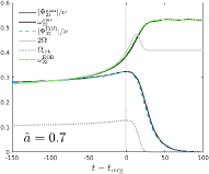
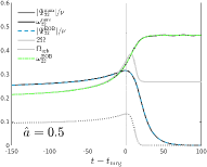
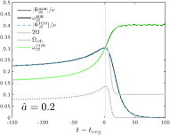
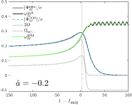
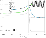
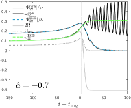
Figure 17: Comparing EOB and numerical amplitude and frequencies in the large-mass-ratio limit ($\nu=10^{-3}$) for different values of the Kerr dimensionless spin parameter $\hat{a}$. As can be seen, $\omega_{22}\simeq 2\Omega$ throughout the whole evolution up to merger. This behavior is also qualitatively shared by TEOBResumS, as shown in Fig. 16. We also show the reliability of the analytical prescription overlapping the EOB amplitudes and frequencies to numerical results.

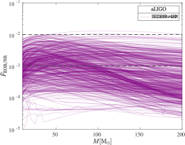
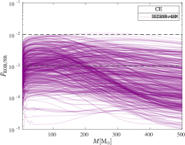
Figure 18: Direct EOB/NR unfaithfulness comparison using the standard implementation of TEOBResumS (top panels) and SEOBNRv4HM (bottom panels). Again, the unfaithfulness is evaluated for the sample of 534 nonprecessing quasicircular NR simulations of the SXS catalog (likewise Fig. 12) using: (i) the zero-detuned, high-power noise spectral density of Advanced LIGO (first column), (ii) the expected PSD for Einstein Telescope (second column), (iii) the expected PSD for Cosmic Explorer (third column).

V.3 Unfaithfulness

Let us finally move to the calculation of the EOB/NR unfaithfulness using the SEOBNRv4HM model. This calculation is not new, since it was done for the first time in Ref. Bohé et al. (2017) as test of the SEOBNRv4 model. However, from Ref. Bohé et al. (2017) several new NR simulations offering a better covering of the parameter space became available and the original $\bar{F}$ calculation was not updated since. In particular, updated comparisons don’t seem to exist in Refs. Cotesta et al. (2018); Ossokine et al. (2020), nor in Ref. Mihaylov et al. (2021), that presents a faster version of the SEOBNRv4HM model based on the application of the post-adiabatic approximation developed in Ref. Nagar and Rettegno (2019) (and notably already applied to the SEOBNRv4HM Hamiltonian in Ref. Rettegno et al. (2019)). To our knowledge, it seems that $\bar{F}_{\rm EOB/NR}$ has never been directly computed all over the 534 spin-aligned datasets currently available. It should be mentioned, though, that there exists a comparison between SEOBNRv4HM and the NR surrogate Pratten et al. (2020). The purpose of this section is to complement the results of Ref. Pratten et al. (2020) via a direct comparison with the SXS datasets. To put this analysis into the right context, we present these results by contrasting them with the corresponding ones obtained using the standard, publicly available, $C$ implementation of TEOBResumS already presented in Ref. Riemenschneider et al. (2021). Since this model relies on fits for the NQC corrections, as detailed in Ref. Riemenschneider et al. (2021), its performance is slightly less good than the one we would obtain by using the (iterated) MATLAB implementation and similarly less good than what is theoretically achievable using TEOBResumS_NQC_lm. Figure 18 directly compares $\bar{F}_{\rm EOB/NR}(M)$ from TEOBResumS (top panels) with the one from SEOBNRv4HM (bottom panels). The calculation is done for Advanced LIGO (first column), ET-D (second column) and CE (third column). The bottom-left panel of Fig. 18 is the analogous of Fig. 2 of Ref. Bohé et al. (2017), but with the additional SXS data that were not available at the time, and highlights the very different behavior of the two models for low masses, where SEOBNRv4HM grazes the $10^{-2}$ level for many configurations. This mirrors intrinsic structural differences, probably connected to the completely different way of deforming the Hamiltonian of a point-particle around a Kerr black hole implemented in the two models Rettegno et al. (2019). If this is acceptable for Advanced LIGO (although it evidences that the SEOBNRv4HM implementation is not accurate enough), it is not acceptable for ET-D or CE1, where SEOBNRv4HM grazes the $10^{-2}$ level for many configurations. Concerning the requirements for third generation detectors, Ref. Pürrer and Haster (2020) concluded that current EOB models are not yet sufficiently accurate. Our analysis shows that things look better by at least one order of magnitude for TEOBResumS or TEOBResumS_NQC_lm, that thus represent more encouraging starting points for developing highly faithful waveform models. Coming back to the Advanced LIGO design sensitivity curve, the results of the two left panels of Fig. 18 are further summarized in Fig. 19, that shows the corresponding $\bar{F}^{\rm max}_{\rm EOB/NR}$ either versus $\tilde{a}_{0}$ or versus $q$. Again, TEOBResumS is quite robust all over the parameter space, although its performance worsens when the effective spin is increased. This clearly indicates where the model needs to be improved further, coherently with the discussion made in the sections above. By contrast, this structure is absent for SEOBNRv4HM points, that look randomly distributed all over the parameter space.

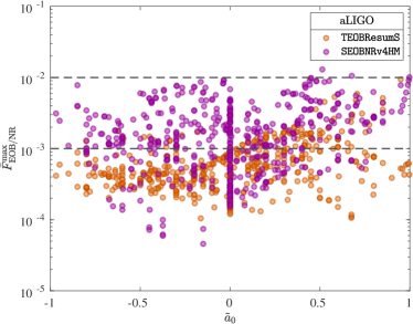
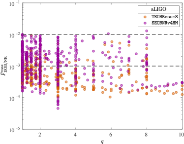
Figure 19: Contrasting $\bar{F}^{\rm max}_{\rm EOB/NR}$ for TEOBResumS and SEOBNRv4HM versus $\tilde{a}_{0}$ and $\nu$. The values for TEOBResumS are smaller than those of SEOBNRv4HM, and also show a clear dependence on the effective spin, indicating where the model may need further improvements.

VI Conclusions

We have presented an updated version of the spin-aligned waveform model TEOBResumS that differs from the previous ones for (i) a more careful procedure to inform the spin sector of the model, including new choices for NR simulations and a different functional form for the fit of the effective spin-orbit parameter $c_{3}$, (ii) a specific effort to improve the behavior of the radiation reaction up to merger. In particular, our main achievement is to show that a careful inclusion of NQC corrections in the flux typically allows to achieve a EOB/NR flux consistency below $1\%$ during the plunge. The consequent recalibration of the spin-orbit sector eventually grants a model that shows a higher NR-faithfulness all over the NR-covered parameter space. In addition we have provided the first ever detailed comparison between TEOBResumS and SEOBNRv4HM. Our results can be summarized as follows.

1. We have presented a novel computation of the angular momentum flux from a selected sample of 36 SXS datasets chosen so as to give a meaningful coverage of the full NR parameter space. Apparently, ours is the first computation of this kind from the early exploration of Ref. Boyle et al. (2008). We have introduced an efficient procedure to remove low-frequency oscillations that are present in the raw fluxes obtained directly from the data. Such oscillations, if kept, would prevent us to perform quantitatively accurate EOB/NR comparisons when the fluxes are represented as functions of the frequency.

2. We have shown that the radiation reaction included in the standard implementation of TEOBResumS Nagar et al. (2020); Riemenschneider et al. (2021) already exhibits an excellent consistency with the NR fluxes. However, this can be further improved by including NQC flux corrections in all $\ell=m$ modes up to $\ell=5$.

3. This modification to the radiation reaction effectively defined a new model, called TEOBResumS_NQC_lm, that also required us to update the determination of the NR-informed effective spin-orbit parameter $c_{3}$. We did so by choosing a new sample of SXS NR datasets, many of which have improved accuracy with respect to the ones used in previous work. We evaluated the performance of this model all over the 534 spin-aligned SXS simulations available, using the Advanced LIGO PSD as well as the ones of ET and CE. To our knowledge, this is the first time an EOB model is being extensively tested for 3G detectors. We found that $\bar{F}_{\rm EOB/NR}$ is within $10^{-4}$ and $10^{-3}$ for more than $80\%$ of the considered binaries. The outliers always occur for configurations with large, positive, spins, that are the most difficult to simulate numerically and to model analytically. Although we are still far from the expected 3G detector calibration error, between $\sim 10^{-4}$ and $\sim 10^{-5}$, our analysis shows that (any version of) TEOBResumS can already be used for 3G-related studies provided the spin parameters are not too extreme. In our opinion, it might be possible that the increase in accuracy needed for 3G detectors advocated in Ref. Pürrer and Haster (2020) will be less dramatic than suggested.

4. By contrast, when the same analyses are performed on the SEOBNRv4HM EOB waveform model, we find large differences between the analytical and numerical fluxes for a restricted sample of dataset for which, however, TEOBResumS is NR-consistent already in its native form. For the same configurations we also considered waveform and frequencies comparisons, underlining how the dynamics of TEOBResumS is qualitatively consistent with the expectations coming from test-particle limit calculations. Similarly, we show that for the same configurations the dynamics of SEOBNRv4HM, differently from the one of TEOBResumS, is qualitatively inconsistent with the expectations coming from test-particle limit calculations. We finally fill the apparent gap in the literature of the calculation of the EOB/NR unfaithfulness for the $\ell=m=2$ mode over all the 534 spin-aligned SXS NR simulations available, for Advanced LIGO, ET-D and CE detectors. The outcome of this calculation is directly contrasted with the corresponding one from the standard version of TEOBResumS, highlighting the different performance of the two models, especially during the inspiral. This is worth noticing because TEOBResumS and SEOBNRv4HM were built using similar strategies and the same original PN information.

The most important take-away message of our work is that TEOBResumS can be improved (especially in the large-spin sector) only by means of minimal modifications to its structure and a more careful choice of the NR simulations used to inform the model. In this respect, it is worth mentioning that the available NR simulations could be better exploited to inform both $a_{6}^{c}$ and $c_{3}$. To maintain continuity with previous work, we did not change the function describing $a_{6}^{c}$ and we anchored the fit of $c_{3}$ to the equal-mass case, using 16 equal-mass SXS dataset, while only additional 20 are used to determine the function up to $q=8$. This was motivated by the fact that in the past the SXS collaboration mainly focused on producing equal-mass binaries. Nowadays things have changed, and in particular there are many dataset available with $q=4$, since they were needed to construct a NR waveform surrogate NRSur7dq4 Varma et al. (2019). Since we are using only 2 dataset with $q\simeq 4$, an improved model would be obtained by just anchoring the $c_{3}$ fit to more $q=4$ simulations, possibly with also an improved choice of $a_{6}^{c}$ more carefully exploiting the nonspinning datasets. We expect that this will additionally improve the EOB/NR agreement, possibly pushing it below the $10^{-4}$ level for all binaries. This seems to be at reach given the simplicity and minimality of our procedures and will be tackled in future work.

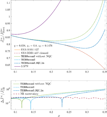
Figure 20: Contrasting EOB/NR total fluxes summed up to $\ell=8$ using either TEOBResumS or TEOBResumS_NQC_lm for the dataset SXS:BBH:1437, with $(q,\chi_{1},\chi_{2})=(6.038,0.8,0.1476)$. The addition of NQC corrections increases the EOB/NR agreement, though it is not sufficient to completely remove the growing behavior at the end of the evolution. As seen in Fig. 8, for TEOBResumS_NQC_lm the multipoles up to $\ell=m=5$ are consistent with the numerical flux, meaning that the improvement is only needed for modes with $\ell\geq 6$.

Appendix A Issues in the NQC-corrected fluxes

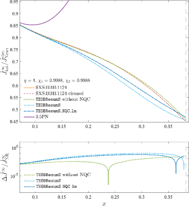
Figure 21: Contrasting EOB/NR fluxes for the configuration $(q,\chi_{1},\chi_{2})=(1,0.9988,0.9988)$, corresponding to dataset SXS:BBH:1124. The flux without NQC corrections is more consistent with the numerical one with respect to the NQC-corrected ones, both from TEOBResumS and from TEOBResumS_NQC_lm.

In this section we focus on some problematic EOB fluxes. Let us start by considering the dataset SXS:BBH:1437. As seen in Fig. 20, for this configuration the additions of NQC corrections increases the agreement with NR but does not avoid the growing behavior at the end of the evolution. As pointed out in Fig. 8, for TEOBResumS_NQC_lm the EOB flux is consistent with the numerical one up to $\ell=m=5$, so this behavior this is due to modes with $6\leq\ell\leq 8$, that only rely on analytical information and do not incorporate NQC corrections. Nevertheless, we underline that the EOB/NR relative difference for TEOBResumS_NQC_lm is of order $10^{-3}$ until $x\sim 0.24$, corresponding to $\sim 1.5$ orbits before merger.

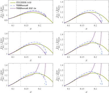
Figure 22: Comparison between EOB/NR fluxes for one of the configurations excluded from Fig. 9, SXS:BBH:1419, with $(q,\chi_{1},\chi_{2})=(8,-0.8,-0.8)$. In this case the NQC correction factor in the $\ell=m=4$ mode becomes pathological and eventually TEOBResumS yields a more NR-consistent flux.

Let us now consider dataset SXS:BBH:1124, corresponding to the extremely spinning configuration $(q,\chi_{1},\chi_{2})=(1,0.9988,0.9988)$. In this case the purely analytical flux is in excellent agreement with the NR one, keeping the fractional difference below $10^{-2}$ until merger, but surprisingly NQC corrections worsen the flux behavior all over the evolution. This may be attributed to two different facts: (i) the motion for a comparable mass binary with such high spins is highly adiabatic, so that there is a reduced need of non-circular correction factors; (ii) NQC corrections in the current model are added from the beginning of the evolution, considering they are functions of the radial momentum which is small but non-negligible during the inspiral, and its effect is progressively amplified. To avoid this issue it seems better to include the NQC factor only as a correction that is progressively switched on towards merger, similarly to what is currently implemented in the version of TEOBResumS valid for noncircular configurations Nagar et al. (2021a); Nagar and Rettegno (2021).

Finally, we consider the two datasets excluded from the bottom panel of Fig. 9, namely SXS:BBH:1419 and SXS:BBH:1375, respectively corresponding to $(q,\chi_{1},\chi_{2})=(8,-0.80,-0.80)$ and $(q,\chi_{1},\chi_{2})=(8,-0.90,0)$. The multipolar fluxes for the first configuration are shown in Fig. 22, from which we infer that the NQC correction factor is not correctly determined for the $\ell=m=4$ and $\ell=m=5$ modes, with the former multipole yielding the largest deviations. One notices, however, that up the $\ell=m=4$ mode excluded, NQC corrections yield an agreement between the fluxes up to the LSO that is closer than the standard case. The same happens for the dataset SXS:BBH:1375. We also found that for $(8,-0.80,-0.80)$ it is possible to fix the behavior of the $\ell=m=4$ mode by adjusting the $c_{3}$ value from the value predicted by the fit, $c_{3}^{\rm fit}=65.16$, to $c_{3}=77$. On the contrary, this is not possible for $(8,-0.90,0)$, indicating that a more detailed understanding of the determination of the NQC corrections is needed in this case.

Appendix B Improving the consistency between waveform and flux changing Newtonian prefactors

Let us finally present an EOB/NR flux comparison using a model that has $\ell=m$ NQC corrections in the flux up to $\ell=5$ and uses consistent Newtonian prefactors in the flux and in the waveform. In practice, this amounts at replacing $v_{\Omega}=\Omega^{1/3}$ with the standard $v_{\varphi}$ in Eqs. (3.22)-(3.30) in Sec. IIIC of Ref. Nagar et al. (2019a). As can be seen in Fig. 23, this actually yields a more consistent flux for the configuration corresponding to dataset SXS:BBH:1436 we analyzed previously. But, not surprisingly, this does not hold for the problematic corner of the parameter space that motivated the different choice for the Newtonian prefactors in the waveform, as evident when looking at the values in Table 4. Moreover, we noticed there are some configurations, e.g. $(8,-0.8,-0.8)$, in which even the $\ell=m=2$ multipole is spoiled by the unsuccessful determination of NQC corrections.

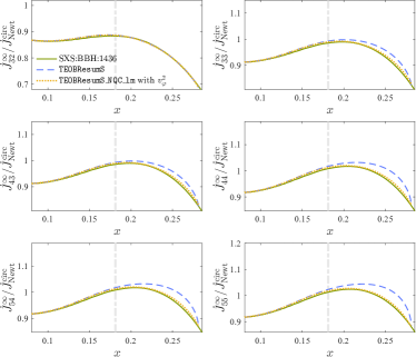
Figure 23: Comparing EOB/NR multipolar fluxes for the dataset SXS:BBH:1436, using TEOBResumS_NQC_lm with the standard Newtonian prefactors in the waveform written as powers of $v_{\varphi}$ (see text). For this configuration, this choice yields an excellent EOB/NR agreement up to merger.

For future developments, the EOB/NR flux agreement in Fig. 23 encourages us to look for different solutions to ensure the NQC determination works out for high mass ratios and negative spins.

Table 4: EOB/NR fractional flux differences at $x=0.2$, both for TEOBResumS_NQC_lm and for its waveform/flux consistent version.

ID	$(q,\chi_{1},\chi_{2})$	$\Delta\dot{J}^{\texttt{NQC\_lm}}_{\rm EOBNR}$	$\Delta\dot{J}^{v_{\varphi}^{2}}_{\rm EOBNR}$
BBH:1155	$(1,0,0)$	$0.001957$	0.0022517
BBH:1222	$(2,0,0)$	$-0.0001001$	0.002563
BBH:1179	$(3,0,0)$	$-0.00071698$	0.0040221
BBH:0190	$(4.499,0,0)$	$-0.0084789$	$-0.0021009$
BBH:0192	$(6.58,0,0)$	$-0.0098679$	$-0.0030977$
BBH:1107	$(10,0,0)$	$-0.011246$	$-0.0096363$
BBH:1137	$(1,-0.97,-0.97)$	$0.099337$	-
BBH:2084	$(1,-0.90,0)$	$0.072879$	0.038549
BBH:2097	$(1,+0.30,0)$	$-0.0032907$	$-0.0029234$
BBH:2105	$(1,+0.90,0)$	$-0.01013$	$-0.011484$
BBH:1124	$(1,+0.99,+0.99)$	$-0.0272$	$-0.027025$
BBH:1146	$(1.5,+0.95,+0.95)$	$-0.035553$	$-0.035553$
BBH:2111	$(2,-0.60,+0.60)$	$0.015314$	$0.017929$
BBH:2124	$(2,+0.30,0)$	$-0.0061851$	$-0.0044956$
BBH:2131	$(2,+0.85,+0.85)$	$-0.01893$	$-0.018629$
BBH:2132	$(2,+0.87,0)$	$-0.011947$	$-0.010621$
BBH:2133	$(3,-0.73,+0.85)$	$0.031988$	0.03876
BBH:2153	$(3,+0.30,0)$	$-0.0042875$	$-0.0012004$
BBH:2162	$(3,+0.60,+0.40)$	$-0.011459$	$-0.0097236$
BBH:1446	$(3.154,-0.80,+0.78)$	0.04242	$0.049673$
BBH:1936	$(4,-0.80,-0.80)$	0.051971	-
BBH:2040	$(4,-0.80,-0.40)$	0.048942	0.063711
BBH:1911	$(4,0,-0.80)$	0.0019117	0.0083588
BBH:2014	$(4,+0.80,+0.40)$	$-0.0089473$	$-0.0078338$
BBH:1434	$(4.368,+0.80,+0.80)$	$-0.012975$	$-0.01188$
BBH:1463	$(4.978,+0.61,+0.24)$	$-0.0083662$	$-0.0064106$
BBH:0208	$(5,-0.90,0)$	$0.037164$	$0.0016289$
BBH:1428	$(5.518,-0.80,-0.70)$	$0.030081$	-
BBH:1437	$(6.038,+0.80,+0.15)$	$-0.001383$	$-0.00033034$
BBH:1436	$(6.281,+0.009,-0.80)$	$-0.002271$	$0.0041482$
BBH:1435	$(6.588,-0.79,+0.7)$	$0.0054703$	-
BBH:1448	$(6.944,-0.48,+0.52)$	$0.0091571$	$0.42486$
BBH:1375	$(8,-0.90,0)$	$1.3589$	-
BBH:1419	$(8,-0.80,-0.80)$	$0.19952$	-
BBH:1420	$(8,-0.80,+0.80)$	$-0.022786$	-
BBH:1455	$(8,-0.40,0)$	$0.0070483$	$0.27028$

Appendix C Unfaithfulness with the ET-C noise

We display in this section results for the EOB/NR unfaithfulness computation by using the less recent PSD of Einstein Telescope, ET-C Hild et al. (2010). As one can see in Fig. 11, ET-D has a larger sensitivity with respect to ET-C for higher frequencies, where we expect both EOB and NR waveforms to be less accurate. Correspondently, the results shown in Fig. 24 and in Table 5 are slightly better than the ones we reported above for the latest PSD, probably also owing to the fact that viceversa the ET-C version has a larger sensitivity at lower frequencies.

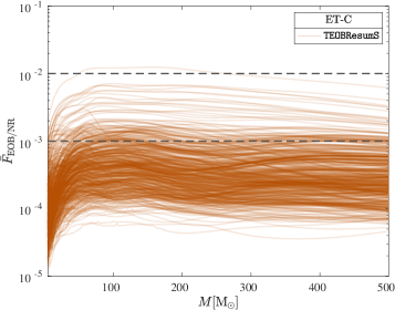
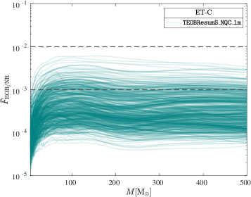
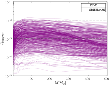
Figure 24: EOB/NR unfaithfulness for TEOBResumS (top), TEOBResumS_NQC_lm (middle) and SEOBNRv4HM (bottom), evaluated using the ET-C version of the expected noise for Einstein Telescope Hild et al. (2010).

Table 5: Analogous of Table 3, using the ET-C power spectral density. The central columns of the table display the fraction of datasets whose maximum unfaithfulness $\bar{F}^{\rm max}_{\rm EOB/NR}$ is within the indicated limits for TEOBResumS, TEOBResumS_NQC_lm or SEOBNRv4HM. Again, as in Table 3, the last two columns display percentage numbers out of all the mismatch values.

	$\bar{F}^{\rm max}<10^{-3}$	$10^{-3}<\bar{F}^{\rm max}<10^{-2}$	$\bar{F}^{\rm max}>3\times 10^{-3}$	$10^{-4}<\bar{F}<10^{-3}$	$\bar{F}<10^{-4}$
TEOBResumS	85.0%	14.4%	2.6%	84.5%	5.3%
TEOBResumS_NQC_lm	82.4%	18.0%	1.7%	81.1%	6.9%
SEOBNRv4HM	36.3%	38.0%	27.7%	48.1%	3.2%

References

- Acernese et al. (2015) F. Acernese et al. (VIRGO), Class. Quant. Grav. 32, 024001 (2015), arXiv:1408.3978 [gr-qc] .
- Aasi et al. (2015) J. Aasi et al. (LIGO Scientific), Class. Quant. Grav. 32, 074001 (2015), arXiv:1411.4547 [gr-qc] .
- Abbott et al. (2021) R. Abbott et al. (LIGO Scientific, Virgo), Phys. Rev. X 11, 021053 (2021), arXiv:2010.14527 [gr-qc] .
- Buonanno and Damour (1999) A. Buonanno and T. Damour, Phys. Rev. D59, 084006 (1999), arXiv:gr-qc/9811091 .
- Buonanno and Damour (2000) A. Buonanno and T. Damour, Phys. Rev. D62, 064015 (2000), arXiv:gr-qc/0001013 .
- Damour et al. (2000) T. Damour, P. Jaranowski, and G. Schaefer, Phys. Rev. D62, 084011 (2000), arXiv:gr-qc/0005034 [gr-qc] .
- Damour (2001) T. Damour, Phys. Rev. D64, 124013 (2001), arXiv:gr-qc/0103018 .
- Damour et al. (2015) T. Damour, P. Jaranowski, and G. Schäfer, Phys. Rev. D91, 084024 (2015), arXiv:1502.07245 [gr-qc] .
- Nagar and Rettegno (2019) A. Nagar and P. Rettegno, Phys. Rev. D99, 021501 (2019), arXiv:1805.03891 [gr-qc] .
- Nagar et al. (2018) A. Nagar et al., Phys. Rev. D98, 104052 (2018), arXiv:1806.01772 [gr-qc] .
- Cotesta et al. (2018) R. Cotesta, A. Buonanno, A. Bohé, A. Taracchini, I. Hinder, and S. Ossokine, Phys. Rev. D98, 084028 (2018), arXiv:1803.10701 [gr-qc] .
- Nagar et al. (2019a) A. Nagar, G. Pratten, G. Riemenschneider, and R. Gamba, (2019a), arXiv:1904.09550 [gr-qc] .
- Nagar et al. (2020) A. Nagar, G. Riemenschneider, G. Pratten, P. Rettegno, and F. Messina, Phys. Rev. D 102, 024077 (2020), arXiv:2001.09082 [gr-qc] .
- Ossokine et al. (2020) S. Ossokine et al., Phys. Rev. D 102, 044055 (2020), arXiv:2004.09442 [gr-qc] .
- Schmidt et al. (2021) S. Schmidt, M. Breschi, R. Gamba, G. Pagano, P. Rettegno, G. Riemenschneider, S. Bernuzzi, A. Nagar, and W. Del Pozzo, Phys. Rev. D 103, 043020 (2021), arXiv:2011.01958 [gr-qc] .
- Chiaramello and Nagar (2020) D. Chiaramello and A. Nagar, Phys. Rev. D 101, 101501 (2020), arXiv:2001.11736 [gr-qc] .
- Nagar et al. (2021a) A. Nagar, A. Bonino, and P. Rettegno, Phys. Rev. D 103, 104021 (2021a), arXiv:2101.08624 [gr-qc] .
- Nagar and Rettegno (2021) A. Nagar and P. Rettegno, (2021), arXiv:2108.02043 [gr-qc] .
- Damour et al. (2014) T. Damour, F. Guercilena, I. Hinder, S. Hopper, A. Nagar, et al., (2014), arXiv:1402.7307 [gr-qc] .
- Nagar et al. (2021b) A. Nagar, P. Rettegno, R. Gamba, and S. Bernuzzi, Phys. Rev. D 103, 064013 (2021b), arXiv:2009.12857 [gr-qc] .
- Gamba et al. (2021a) R. Gamba, M. Breschi, G. Carullo, P. Rettegno, S. Albanesi, S. Bernuzzi, and A. Nagar, Submitted to Nature Astronomy (2021a), arXiv:2106.05575 [gr-qc] .
- Pratten et al. (2020) G. Pratten, S. Husa, C. Garcia-Quiros, M. Colleoni, A. Ramos-Buades, H. Estelles, and R. Jaume, Phys. Rev. D 102, 064001 (2020), arXiv:2001.11412 [gr-qc] .
- García-Quirós et al. (2020) C. García-Quirós, M. Colleoni, S. Husa, H. Estellés, G. Pratten, A. Ramos-Buades, M. Mateu-Lucena, and R. Jaume, Phys. Rev. D 102, 064002 (2020), arXiv:2001.10914 [gr-qc] .
- Pratten et al. (2021) G. Pratten et al., Phys. Rev. D 103, 104056 (2021), arXiv:2004.06503 [gr-qc] .
- Akcay et al. (2021) S. Akcay, R. Gamba, and S. Bernuzzi, Phys. Rev. D 103, 024014 (2021), arXiv:2005.05338 [gr-qc] .
- Gamba et al. (2021b) R. Gamba, S. Akçay, S. Bernuzzi, and J. Williams, (2021b), arXiv:2111.03675 [gr-qc] .
- Rettegno et al. (2019) P. Rettegno, F. Martinetti, A. Nagar, D. Bini, G. Riemenschneider, and T. Damour, (2019), arXiv:1911.10818 [gr-qc] .
- Damour et al. (2012) T. Damour, A. Nagar, D. Pollney, and C. Reisswig, Phys.Rev.Lett. 108, 131101 (2012), arXiv:1110.2938 [gr-qc] .
- Nagar et al. (2016) A. Nagar, T. Damour, C. Reisswig, and D. Pollney, Phys. Rev. D93, 044046 (2016), arXiv:1506.08457 [gr-qc] .
- Ossokine et al. (2018) S. Ossokine, T. Dietrich, E. Foley, R. Katebi, and G. Lovelace, Phys. Rev. D98, 104057 (2018), arXiv:1712.06533 [gr-qc] .
- Le Tiec et al. (2011) A. Le Tiec, A. H. Mroue, L. Barack, A. Buonanno, H. P. Pfeiffer, N. Sago, and A. Taracchini, Phys. Rev. Lett. 107, 141101 (2011), arXiv:1106.3278 [gr-qc] .
- Le Tiec et al. (2013) A. Le Tiec et al., Phys. Rev. D 88, 124027 (2013), arXiv:1309.0541 [gr-qc] .
- Hinderer et al. (2013) T. Hinderer et al., Phys. Rev. D88, 084005 (2013), arXiv:1309.0544 [gr-qc] .
- Boyle et al. (2008) M. Boyle, A. Buonanno, L. E. Kidder, A. H. Mroue, Y. Pan, et al., Phys.Rev. D78, 104020 (2008), arXiv:0804.4184 [gr-qc] .
- Boyle et al. (2019) M. Boyle et al., Class. Quant. Grav. 36, 195006 (2019), arXiv:1904.04831 [gr-qc] .
- Reitze et al. (2021) D. Reitze et al., (2021), arXiv:2111.06986 [gr-qc] .
- Couvares et al. (2021) P. Couvares et al., (2021), arXiv:2111.06987 [gr-qc] .
- Punturo et al. (2021) M. Punturo et al., (2021), arXiv:2111.06988 [gr-qc] .
- Katsanevas et al. (2021) S. Katsanevas et al., (2021), arXiv:2111.06989 [gr-qc] .
- Kalogera et al. (2021) V. Kalogera et al., (2021), arXiv:2111.06990 [gr-qc] .
- McClelland et al. (2021) D. McClelland et al., (2021), arXiv:2111.06991 [gr-qc] .
- Damour and Nagar (2014) T. Damour and A. Nagar, Phys.Rev. D90, 044018 (2014), arXiv:1406.6913 [gr-qc] .
- (43) “Updated Advanced LIGO sensitivity design curve,” https://dcc.ligo.org/LIGO-T1800044/public.
- Hild et al. (2010) S. Hild, S. Chelkowski, A. Freise, J. Franc, N. Morgado, R. Flaminio, and R. DeSalvo, Class. Quant. Grav. 27, 015003 (2010), arXiv:0906.2655 [gr-qc] .
- Hild et al. (2011) S. Hild et al., Class. Quant. Grav. 28, 094013 (2011), arXiv:1012.0908 [gr-qc] .
- Evans et al. (2021) M. Evans et al., (2021), arXiv:2109.09882 [astro-ph.IM] .
- Bohé et al. (2017) A. Bohé et al., Phys. Rev. D95, 044028 (2017), arXiv:1611.03703 [gr-qc] .
- Cotesta et al. (2020) R. Cotesta, S. Marsat, and M. Pürrer, Phys. Rev. D 101, 124040 (2020), arXiv:2003.12079 [gr-qc] .
- Mitman et al. (2021) K. Mitman et al., Phys. Rev. D 104, 024051 (2021), arXiv:2105.02300 [gr-qc] .
- Campanelli et al. (2006) M. Campanelli, C. Lousto, and Y. Zlochower, Phys.Rev. D74, 041501 (2006), arXiv:gr-qc/0604012 [gr-qc] .
- Bini and Damour (2012) D. Bini and T. Damour, Phys.Rev. D86, 124012 (2012), arXiv:1210.2834 [gr-qc] .
- Damour and Gopakumar (2006) T. Damour and A. Gopakumar, Phys. Rev. D73, 124006 (2006), arXiv:gr-qc/0602117 .
- Damour and Nagar (2007) T. Damour and A. Nagar, Phys. Rev. D76, 064028 (2007), arXiv:0705.2519 [gr-qc] .
- Damour et al. (2013) T. Damour, A. Nagar, and S. Bernuzzi, Phys.Rev. D87, 084035 (2013), arXiv:1212.4357 [gr-qc] .
- Damour et al. (2009) T. Damour, B. R. Iyer, and A. Nagar, Phys. Rev. D79, 064004 (2009), arXiv:0811.2069 [gr-qc] .
- Nagar et al. (2017) A. Nagar, G. Riemenschneider, and G. Pratten, Phys. Rev. D96, 084045 (2017), arXiv:1703.06814 [gr-qc] .
- Riemenschneider et al. (2021) G. Riemenschneider, P. Rettegno, M. Breschi, A. Albertini, R. Gamba, S. Bernuzzi, and A. Nagar, Phys. Rev. D 104, 104045 (2021), arXiv:2104.07533 [gr-qc] .
- Damour and Nagar (2009) T. Damour and A. Nagar, Phys. Rev. D79, 081503 (2009), arXiv:0902.0136 [gr-qc] .
- Pürrer and Haster (2020) M. Pürrer and C.-J. Haster, Phys. Rev. Res. 2, 023151 (2020), arXiv:1912.10055 [gr-qc] .
- Moxon et al. (2021) J. Moxon, M. A. Scheel, S. A. Teukolsky, N. Deppe, N. Fischer, F. Hébert, L. E. Kidder, and W. Throwe, (2021), arXiv:2110.08635 [gr-qc] .
- Fischer et al. (2021) N. L. Fischer et al., (2021), arXiv:2111.06767 [gr-qc] .
- Zertuche et al. (2021) L. M. n. Zertuche et al., (2021), arXiv:2110.15922 [gr-qc] .
- Albanesi et al. (2021) S. Albanesi, A. Nagar, and S. Bernuzzi, Phys. Rev. D 104, 024067 (2021), arXiv:2104.10559 [gr-qc] .
- Harms et al. (2014) E. Harms, S. Bernuzzi, A. Nagar, and A. Zenginoglu, Class.Quant.Grav. 31, 245004 (2014), arXiv:1406.5983 [gr-qc] .
- Barausse et al. (2012) E. Barausse, A. Buonanno, S. A. Hughes, G. Khanna, S. O’Sullivan, et al., Phys.Rev. D85, 024046 (2012), arXiv:1110.3081 [gr-qc] .
- Taracchini et al. (2013) A. Taracchini, A. Buonanno, S. A. Hughes, and G. Khanna, Phys.Rev. D88, 044001 (2013), arXiv:1305.2184 [gr-qc] .
- Mihaylov et al. (2021) D. P. Mihaylov, S. Ossokine, A. Buonanno, and A. Ghosh, (2021), arXiv:2105.06983 [gr-qc] .
- Barausse et al. (2009) E. Barausse, E. Racine, and A. Buonanno, Phys. Rev. D80, 104025 (2009), arXiv:0907.4745 [gr-qc] .
- Barausse and Buonanno (2010) E. Barausse and A. Buonanno, Phys.Rev. D81, 084024 (2010), arXiv:0912.3517 [gr-qc] .
- Barausse and Buonanno (2011) E. Barausse and A. Buonanno, Phys.Rev. D84, 104027 (2011), arXiv:1107.2904 [gr-qc] .
- Varma et al. (2019) V. Varma, S. E. Field, M. A. Scheel, J. Blackman, D. Gerosa, L. C. Stein, L. E. Kidder, and H. P. Pfeiffer, Phys. Rev. Research. 1, 033015 (2019), arXiv:1905.09300 [gr-qc] .
- Nagar et al. (2019b) A. Nagar, F. Messina, P. Rettegno, D. Bini, T. Damour, A. Geralico, S. Akcay, and S. Bernuzzi, Phys. Rev. D99, 044007 (2019b), arXiv:1812.07923 [gr-qc] .