Throughput Maximization for IRS-Aided MIMO FD-WPCN with Non-Linear EH Model

Abstract

This paper studies an intelligent reflecting surface (IRS)-aided multiple-input-multiple-output (MIMO) full-duplex (FD) wireless-powered communication network (WPCN), where a hybrid access point (HAP) operating in FD broadcasts energy signals to multiple devices for their energy harvesting (EH) in the downlink (DL) and meanwhile receives information signals from devices in the uplink (UL) with the help of an IRS. Taking into account the practical finite self-interference (SI) and the non-linear EH model, we formulate the weighted sum throughput maximization optimization problem by jointly optimizing DL/UL time allocation, precoding matrices at devices, transmit covariance matrices at the HAP, and phase shifts at the IRS. Since the resulting optimization problem is non-convex, there are no standard methods to solve it optimally in general. To tackle this challenge, we first propose an element-wise (EW) based algorithm, where each IRS phase shift is alternately optimized in an iterative manner. To reduce the computational complexity, a minimum mean-square error (MMSE) based algorithm is proposed, where we transform the original problem into an equivalent form based on the MMSE method, which facilities the design of an efficient iterative algorithm. In particular, the IRS phase shift optimization problem is recast as an second-order cone program (SOCP), where all the IRS phase shifts are simultaneously optimized. For comparison, we also study two suboptimal IRS beamforming configurations in simulations, namely partially dynamic IRS beamforming (PDBF) and static IRS beamforming (SBF), which strike a balance between the system performance and practical complexity. Simulation results demonstrate the effectiveness of proposed two algorithms. Besides, the results show the superiority of our proposed scheme over other benchmark schemes and also unveil the importance of the joint design of passive beamforming and resource allocation for achieving energy efficient MIMO FD-WPCNs.

I Introduction

Wireless communication via radio-frequency (RF) radiation has significantly shaped the people daily life in the past decades. Wireless radio is not limited to forward information-carrying signal transmission and its broadcasting signals can also be utilized by Internet-of-Things (IoT) devices, such as temperature sensors, humidity sensors, and illuminating light sensors, etc., to power the embedded battery [1]. This RF transmission enabled wireless energy transfer (WET) has attracted increasing attention due to its great convenience as well as perpetual supply compared to the intermittent ambient energy harvesting (EH) technologies such as solar, thermal, vibration, etc. There are mainly two paradigms of research on WET in the literature. One is the simultaneous wireless information and power transfer (SWIPT), where IoT devices can receive information and energy simultaneously via the same transmitted signal. The other is the wireless-powered communication network (WPCN), where IoT devices communicate with a hybrid access point (HAP) using the energy harvested from WET. However, for the WPCN, it suffers a “doubly-near-far” phenomenon, where a device far from the HAP receives less wireless energy than a nearer user in the downlink (DL), and has to consume more power in the uplink (UL) for wireless information transmission (WIT) [2]. Therefore, the low efficiencies of WET and WIT for IoT devices over long transmission distances fundamentally limit the performance of practical WPCNs.

To address this “doubly-near-far” issue, intensive research efforts have been made to focus on the design of WPCNs from several aspects such as resource allocation, multiple-input-multiple-output (MIMO), and HAP operation modes in the past. For example, references [3] and [4] studied the joint design of time allocation and transmit power to maximize the sum throughput in WPCNs. However, the above works assumed that the HAP as well as users is equipped with single antenna, which limits both the DL and UL transmission efficiency. To exploit large array gains brought by multiple antennas, the MIMO technology is then integrated in WPCNs, where the HAP and devices are equipped with multiple antennas. To be specific, with multiple antennas at the HAP, a narrow beam can be created and steered towards to devices for their EH with high beamforming gains, and the data transmission rate from devices to the HAP can be remarkably increased due to the additional spatial multiplex/diversity gain [5], [6]. Although the MIMO WPCN is expected to achieve much higher spectral efficiency than the traditional single-input-single-output (SISO) WPCN, substantial works assume that the operations for DL WET and UL WIT are orthogonal over time, i.e, the HAP operates in a half-duplex (HD) mode, which fundamentally limits the system performance. To further improve the utilization of the time resource, the full-duplex (FD) WPCN was proposed in [7, 8, 9, 10], where the HAP operates in an FD mode. In particular, reference [7] was the first work to study SISO FD-WPCN, where the authors proposed an efficient transmission protocol to support simultaneous DL WET and UL WIT and also studied the weighted sum throughput maximization problem by jointly optimizing time allocation and power transmit. The MIMO FD-WPCN was further studied in [10], where the authors focused on a point-to-point system to achieve its rate-region profile by the joint design of the base station beamformer and the time splitting. However, such above techniques cause huge energy consumption and the green technique for realizing a sustainable wireless network evolution is imperative.

Recently, intelligent reflecting surfaces (IRSs) have been proposed as a promising cost-effective solution to improve both spectral- and energy-efficiency of wireless communication systems[11, 12, 13]. The IRS is a two-dimensional planar array comprising a large number of of sub-wavelength metallic or dielectric scatterers, each of which is able to independently manipulate impinging signals by changing their phases and/or amplitudes so that the signals reflected by the IRS can be coherently added up at desired receivers to boost the received power, while destructively added up at non-intended receivers to suppress co-channel interference. In particular, massive reflecting elements can be installed at the IRS due to the small size of each reflecting element, which are able to provide significant passive gains to compensate the high signal attenuation over long distance [13]. The seminal work in [14] unveiled the fundamental scaling law of the IRS by showing that the received signal-to-noise ratio (SNR) increases quadratically with the number of IRS reflecting elements. Inspired by this fundamental insight, IRS-aided wireless communications have been intensively studied for various system setups including physical layer security [15, 16, 17], multi-cell cooperation [18, 19, 20], non-orthogonal multiple access (NOMA) [21, 22, 23]. While most of existing works focus on the IRS-aided WIT, the IRS is also appealing for WET [24, 25, 26, 27]. First, due to the large aperture of IRS, the signals reflected by the properly reconfigured IRS can be coherently added up with the non-IRS reflected signals at the desired devices/HAP to substantially boost DL WET and UL WIT. Second, the energy consumption and the hardware cost of IRS are very low and cheap since the IRS reflecting elements only passively reflect impinging signals without requiring any transmit RF chains. Thus, its energy consumption is typically several orders-of-magnitude lower than that of traditional active antenna arrays [28].

By far, there are only a handful of works paying attention to studying IRS-aided WPCNs [29, 30, 31, 32, 33, 34, 35, 36]. For example, a new dynamic IRS beamforming for WPCNs was proposed to compromise the system performance and implementation complexity in [29]. The results in these works showed that with the joint optimization of IRS phase shifts and resource allocation, the system performance can be significantly improved. However, these works adopted the linear energy harvesting (EH) model for DL WET and ignored the EH saturation caused by practically non-linear rectifiers [37]. Specifically, it was shown that the output direct current (DC) power stored in the embedded battery at devices does not linearly scale with the input RF power, especially as the input RF power level increases, the output DC power will become saturated gradually. As a result, employing a linear EH model may lead to mismatched beamforming and resource allocation results for WPCNs with practical non-linear rectifiers. Moreover, all above works focused on the HD system, which suffers from low spectral efficiency. We note that although the FD technique applied in IRS-aided wireless communication networks has been studied in [38, 39, 40], these works assumed that the self-interference (SI) at the HAP is either a constant or is perfectly cancelled by ignoring the practical quantization error introduced by the strong SI under the limited dynamic range of the analog-to-digital conversion. The research on the joint design of FD and IRS technologies under practical constraints in MIMO WPCNs are still an open problem, which thus motivates this work.

Figure 1: An IRS-aided MIMO FD-WPCN.

In this paper, we study an IRS-aided MIMO FD-WPCN for further improving the system throughput as shown in Fig. 1. The HAP operates in the FD mode and is equipped with two sets of antennas, which are used for DL WET and UL WIT, respectively, and each device is equipped with multiple antennas. The devices harvest energy from the HAP and use the harvested energy to transmit their own information to the HAP with the help of IRS. To the best of our knowledge, it is the first work to study the IRS-aided MIMO FD-WPCN by taking into account the finite SI and the non-linear EH model. Our work is significantly different from the IRS-aided SISO FD-WPCN proposed in [41] mainly from three aspects. First, the extension from the SISO system to the MIMO system resulting in a different problem formulation, thus we propose two new algorithms to cater to the new formulated problem. Second, we adopt a more practical EH model, i.e., the non-linear EH model, rather than the ideal EH model, i.e., the linear EH model, to capture the dynamics of the RF energy conversion efficiency for different input power levels. Third, we propose a novel DL transmission protocol, where a dynamic IRS beamforming (DBF) strategy is proposed to adapt to different channel fading among devices in the DL WET. Moreover, compared to the IRS-aided MIMO HD-WPCN [34], our work differs significantly in terms of transmission protocols, transmitter/receiver architectures, EH constraints, design objectives, and optimization methods. The main contributions of this paper are summarized as follows.

• We study an IRS-aided MIMO FD-WPCN considering practical cases with the finite SI and the non-linear EH model. Our objective is to maximize the weighted sum throughput by jointly optimizing DL/UL time allocation, precoding matrices at devices, transmit covariance matrices at the HAP, and phase shifts at the IRS. Since the resulting optimization problem is non-convex, there are no standard convex methods to solve it optimally. To efficiently solve it, two different algorithms, namely element-wise (EW) based algorithm and minimum mean-square error (MMSE) based algorithm, are proposed to strike a balance between the system performance and the computational complexity.

• For the proposed EW-based algorithm, the original optimization problem is decomposed into several subproblems, namely DL/UL time allocation subproblem, precoding matrices and transmit covariance matrices subproblem, and IRS phase shift subproblem. Then, we alternately optimize each subproblem in an iterative way until convergence is achieved. In particular, for the IRS phase shift optimization, we alternately optimize each phase shift with other phase shifts are fixed. Although the proposed EW-based algorithm provides a good system performance as shown in simulation results, it requires procedures for updating each phase shift in a one-by-one manner.

• To reduce the computational complexity, the MMSE-based algorithm is proposed. Specifically, the original optimization problem is first equivalently transformed into a more tractable form based on the MMSE method. Based on the newly formulated optimization problem, the IRS phase shift optimization problem is recast as a standard second-order cone program (SOCP) by applying the successive convex approximation (SCA) technique, which can be solved with much lower complexity.

• Simulation results demonstrate the benefits of the IRS used for enhancing the performance of the MIMO FD-WPCN, especially when the DBF scheme is adopted for both DL WET and UL WIT. In addition, the IRS-aided MIMO FD-WPCN is able to achieve significantly performance gain compared to the IRS-aided MIMO HD-WPCN when the SI is well suppressed. Furthermore, it is interesting to find that while the DBF is useful for UL WIT, it may not be necessary for DL WET, which helps reduce the implementation complexity in practice.

The rest of this paper is organized as follows. Section II introduces the system model and problem formulation for the IRS-aided MIMO FD-WPCN. In Section III, we propose an EW-based algorithm. In Section IV, we propose an MMSE-based algorithm. Numerical results are provided in Section V and the paper is concluded in Section VI.

Notations: Boldface upper-case and lower-case letters denote matrix and vector, respectively. ${\mathbb{C}}^{d_{1}\times d_{2}}$ stands for the set of complex $d_{1}\times d_{2}$ matrices. For a complex-valued vector $\bf x$, ${\rm diag}(\bf x)$ denotes a diagonal matrix whose main diagonal elements are extracted from vector $\bf x$. For a matrix $\bf X$, ${\bf X}^{*}$, ${\bf X}^{H}$, and ${\rm{tr}}\left({\bf{X}}\right)$ respectively stand for its conjugate, conjugate transpose, and trace, while ${\bf{X}}\succeq{\bf{0}}$ indicates that matrix $\bf X$ is positive semi-definite. ${\bf{X}}\left(\bf x\right)\sim{\cal CN}\left({{\bm{\Upsilon}}\left(\bm{\mu}\right),{\bf{\Sigma}}}\right)$ denotes a circularly symmetric complex Gaussian matrix (vector) with mean $\bm{\Upsilon}\left(\bm{\mu}\right)$ and covariance matrix $\bm{\Sigma}$. ${\mathbb{E}}(\cdot)$ denotes the expectation operation. $\odot$ and $\otimes$ represent the Hadamard product and Kronecker product, respectively. ${\cal O}\left(\cdot\right)$ denotes the big-O computational complexity notation.

II System Model and Problem Formulation

II-A System Model

Consider an IRS-aided FD-WPCN consisting of an HAP, $K$ devices, and an IRS, as shown in Fig. 1. We assume that the HAP operates in the FD mode and the total number of antennas at the HAP is $N_{t}+N_{r}$, of which $N_{t}$ transmit antennas are used for broadcasting energy to the distributed devices in the DL and $N_{r}$ receive antennas are dedicated to receiving information from the distributed devices in the UL simultaneously over the same frequency band. In addition, we assume that the IRS has $M$ reflecting elements and each device has $N_{d}$ antennas.

Figure 2: Transmission protocol for DL WET and UL WIT in the considered MIMO FD-WPCN.

We consider a quasi-static flat-fading channel in which the channel state information (CSI) remains constant in a channel coherence frame, but may change in the subsequent frames. As shown in Fig. 2, each channel coherence frame consists of multiple blocks and each transmission period of one block of interest denoted by $T$ is divided into $K+1$ time slots, each with duration of $\tau_{i},i\in{\cal K}_{1}$, such that $T=\sum\limits_{i=0}^{K}{{\tau_{i}}}$, where ${\cal K}_{1}=\{0,\dots,K\}$. The $0$th time slot is a dedicated time slot used to broadcast energy to all distributed devices in the DL, while the $i$th ($i\neq 0$) time slot is used for UL WIT. The DBF scheme for DL WET is proposed as shown in Fig. 3. Without loss of generality, the $0$th time slot is further divided into $K$ sub-slots with the duration of the $j$th sub-slot denoted by $\tau_{0j},j\in{\cal K}_{2}$, such that ${\tau_{0}}=\sum\limits_{j=1}^{{K}}{{\tau_{0j}}}$, where ${\cal K}_{2}=\{1,\dots,K\}$. Then, each sub-slot is assigned an exclusive IRS phase-shift vector. For ease of exposition, we assume that the $k$th $(k\neq 0)$ time slot is occupied by device $k$ for UL WIT, $k\in{\cal K}_{2}$. Since there are two sets of antennas at the HAP, the DL and UL channels are different in general. In the DL transmission, denote by ${\bf{G}}\in{{\mathbb{C}}^{M\times N_{t}}}$, ${\bf{H}}_{r,k}\in{{\mathbb{C}}^{N_{d}\times M}}$, and ${{\bf H}_{d,k}}\in{{\mathbb{C}}^{N_{d}\times N_{t}}}$ the complex equivalent baseband channel between the HAP and the IRS, between the IRS and the $k$th device, and between the HAP and the $k$th device, $k\in{\cal K}_{2}$, respectively. In the UL transmission, denote by ${\bf{\bar{G}}}\in{{\mathbb{C}}^{N_{r}\times M}}$, ${\bf{\bar{H}}}_{r,k}\in{{\mathbb{C}}^{M\times N_{d}}}$, and ${{\bar{\bf H}}_{d,k}}\in{{\mathbb{C}}^{N_{r}\times N_{d}}}$ the complex equivalent baseband channel between the HAP and the IRS, between the IRS and the $k$th device, and between the HAP and the $k$th device, $k\in{\cal K}_{2}$, respectively. In addition, the channel reciprocity is assumed and thus we have ${{{\bf{\bar{H}}}}_{r,k}}={\bf{H}}_{r,k}^{T}$ for the IRS-device link, $k\in{\cal K}_{2}$.

Figure 3: The DBF scheme for DL/UL time allocation and IRS phase-shift vectors assignment.

II-A1 DL WET

As shown in Fig. 3, each sub-slot in the $0$th time slot is assigned an exclusive IRS phase-shift vector. As such, the received signal by device $k$ in the $i$th sub-slot of time slot $0$ is given by

$${\bf{y}}_{k,i}^{d}=\left({{{\bf{H}}_{d,k}}+{{\bf{H}}_{r,k}}{{\bf{\Theta}}_{i}^{0}}{\bf{G}}}\right){{\bf{x}}_{i}^{0}}+{\bf{n}}_{k,i}^{d},i\in{\cal K}_{2},k\in{\cal K}_{2},$$ (1)

where ${{\bf{x}}_{i}^{0}}$ represents for the HAP’s transmit energy signal in the $i$th sub-slot of time slot $0$ with covariance matrix ${{\bf{Q}}_{i}^{0}}={\mathbb{E}}\left\{{{{\bf{x}}_{i}^{0}}{\bf{x}}_{i}^{0,H}}\right\}\succeq{\bf{0}}$. ${{\bf{\Theta}}_{i}^{0}}={\rm{diag}}\left({{v_{i,1}^{0}},\cdots,{v_{i,M}^{0}}}\right)$ represents a diagonal IRS reflection coefficient matrix in the $i$th sub-slot of time slot $0$, where ${{v_{i,m}^{0}}}$ denotes its $m$th phase shift, and ${\bf n}_{{k},i}^{d}\sim{\cal CN}\left({{\bf 0},\sigma^{2}{\bf I}_{N_{r}}}\right)$ stands for the additive white Gaussian noise. It is worth noting that we consider a periodic transmission protocol as shown in Fig. 2, where each device $k$ can harvest energy during all time slots except its own transmission time slot $k$[7]. Specifically, the energy harvested by device $k$ after its own WIT in the previous transmission block will be used for its WIT in the next transmission block. Under this protocol, the amount of harvested energy by device $k$ during $T$ by using the practical EH model is given by [43], [44]

$${E_{k}}= \sum\limits_{i=1}^{K}{{\tau_{0i}}\left({\frac{{{X_{k}}}}{{1+{e^{-{a_{k}}\left({{\rm{tr}}\left({{\bf{H}}_{k,i}^{0}{\bf{Q}}_{i}^{0}{\bf{H}}_{k,i}^{0,H}}\right)-{b_{k}}}\right)}}}}-{Y_{k}}}\right)}+$$

$$\sum\limits_{j=1,j\neq k}^{K}{{\tau_{j}}\left({\frac{{{X_{k}}}}{{1+{e^{-{a_{k}}\left({{\rm{tr}}\left({{{\bf{H}}_{k,j}}{{\bf{Q}}_{j}}{\bf{H}}_{k,j}^{H}}\right)-{b_{k}}}\right)}}}}-{Y_{k}}}\right)},k\in{\cal K}_{2},$$ (2)

where ${\bf{H}}_{k,i}^{0}={{\bf{H}}_{d,k}}+{{\bf{H}}_{r,k}}{\bf{\Theta}}_{i}^{0}{\bf{G}}$ and ${{\bf{H}}_{k,j}}={{\bf{H}}_{d,k}}+{{\bf{H}}_{r,k}}{{\bf{\Theta}}_{j}}{\bf{G}}$. ${\bf Q}_{j}\succeq{\bf 0}$ stands for the transmit covariance matrix at the HAP in time slot $j$, and ${{\bf{\Theta}}_{j}}={\rm{diag}}\left({{v_{j,1}},\ldots,{v_{j,M}}}\right)$ denotes the IRS phase-shift matrix assigned in time slot $j$, $j\in{\cal K}_{2}$. In addition, $a_{k}$, $b_{k}$, $M_{k}$, ${X_{k}}={M_{k}}\left({1+{e^{{a_{k}}{b_{k}}}}}\right)/{e^{{a_{k}}{b_{k}}}}$, and ${Y_{k}}={{{M_{k}}}}/{{{e^{{a_{k}}{b_{k}}}}}}$ represent device $k$’s circuit configurations, which are related to the resistance, capacitance, diode turn-on voltage, etc.

II-A2 UL WIT

During UL WIT, each device transmits its own to the HAP in a time-division multiple access manner. As such, the received signal at the HAP in time slot $k$ is given by

$${\bf{y}}_{k}^{r}=\underbrace{\left({{{{\bf{\bar{H}}}}_{d,k}}+{\bf{\bar{G}}}{{\bf{\Theta}}_{k}}{{{\bf{\bar{H}}}}_{r,k}}}\right){{\bf{W}}_{k}}{{\bf{s}}_{k}}}_{{\rm{desired}}\;{\rm{signal}}}+\underbrace{\left({{{\bf{H}}_{{\rm{SI}}}}+{\bf{\bar{G}}}{{\bf{\Theta}}_{k}}{\bf{G}}}\right){{\bf{x}}_{k}}}_{{\rm{interference}}}+{\bf{n}}_{k}^{r},k\in{\cal K}_{2},$$ (3)

where ${{\bf{x}}_{k}}\in{\mathbb{C}}^{N_{t}\times 1}$ denotes the energy signal transmitted by the HAP with the transmit covariance matrix denoted by ${{\bf{Q}}_{k}}\succeq{\bf{0}}$ in time slot $k$. ${{\bf{s}}_{k}}\in{{\mathbb{C}}^{{N_{d}}\times 1}}$ represents $N_{d}$ desired data streams for device $k$ satisfying ${{\bf{s}}_{k}}\sim{\cal CN}\left({{\bf{0}},{{\bf{I}}_{d}}}\right)$ and ${{{\bf{W}}_{k}}}\in{\mathbb{C}}^{N_{d}\times N_{d}}$ stands for the transmit beamforming matrix for device $k$. ${{{\bf{H}}_{{\rm SI}}}}\in{\mathbb{C}}^{N_{r}\times N_{t}}$ represents the SI channel from the transmit antennas to the receive antennas at the FD-HAP, and ${\bf n}_{k}^{r}\sim{\cal CN}\left({{\bf 0},\sigma^{2}{\bf I}_{N_{r}}}\right)$ denotes the received additive white Gaussian noise. It can be observed that the interference in (3) consists of two parts. The first term ${{\bf{H}}_{\rm SI}}{{\bf{x}}_{k}}$ denotes the SI resulting from the DL transmission by the HAP and the second term ${\bf{\bar{G}}}{{\bf{\Theta}}_{k}}{\bf{G}}{{\bf{x}}_{k}}$ denotes the interference introduced by the reflection of the DL transmit signal by the IRS. By deploying the IRS close to devices and far from the HAP, the following two benefits can be achieved. First, when the IRS is deployed close to devices, the double propagation loss of the cascaded HAP-IRS-device link will be substantially reduced, which is beneficial for improving the SNR. Second, when the IRS is deployed far from the HAP, the interference introduced by the reflection link, i.e., HAP-IRS-HAP link, will be significantly small and thus can be ignored. Thus, we can simplify (3) as

$${\bf{\hat{y}}}_{k}^{r}={{{\bf{\bar{H}}}}_{k}}{\bf W}_{k}{{\bf{s}}_{k}}+{{\bf{H}}_{{\rm{SI}}}}{{\bf{x}}_{k}}+{\bf{n}}_{k}^{r},k\in{\cal K}_{2},$$ (4)

where ${{{\bf{\bar{H}}}}_{k}}={{{\bf{\bar{H}}}}_{d,k}}+{\bf{\bar{G}}}{{\bf{\Theta}}_{k}}{{{\bf{\bar{H}}}}_{r,k}}$. As a result, the achievable throughput of device $k$ at time slot $k$ can be expressed as

$${R_{k}}={\tau_{k}}\ln\left|{{{\bf{I}}_{{N_{r}}}}+{{{\bf{\bar{H}}}}_{k}}{{\bf{W}}_{k}}{{\bf{W}}_{k}^{H}}{\bf{\bar{H}}}_{k}^{H}{{\left({{{\bf{H}}_{{\rm{SI}}}}{{\bf{Q}}_{k}}{\bf{H}}_{{\rm{SI}}}^{H}+{\sigma^{2}}{{\bf{I}}_{{N_{r}}}}}\right)}^{-1}}}\right|.$$ (5)

II-B Problem Formulation

Define ${{\bf{v}}_{i}^{0}}={\left[{{v_{i,1}^{0}},\ldots,{v_{i,M}^{0}}}\right]^{T}}$ and ${{\bf{v}}_{i}}={\left[{{v_{i,1}},\ldots,{v_{i,M}}}\right]^{T}},i\in{\cal K}_{2}$. Denote by sets ${\cal M}=\left\{{1,\ldots,M}\right\}$, $\tau{\rm{=}}\left\{{\tau_{0,k}}\cup{{\tau_{k}},k\in{{\cal K}_{2}}}\right\}$, ${\bf{W}}=\left\{{{{\bf{W}}_{k}},k\in{{\cal K}_{2}}}\right\}$, ${\bf{v}}=\left\{{{{\bf{v}}_{i}^{0}}\cup{{\bf{v}}_{i}},i\in{{\cal K}_{2}}}\right\}$, and ${\bf{Q}}=\left\{{{{\bf{Q}}_{i}^{0}}\cup{{\bf{Q}}_{i}},i\in{{\cal K}_{2}}}\right\}$. The objective of this paper is to maximize the weighted sum throughput of the IRS-aided MIMO FD-WPCN by jointly optimizing DL/UL time allocation, precoding matrices at devices, transmit covariance matrices at the HAP, and phase-shift vectors at the IRS. Accordingly, the problem is formulated as

$$\mathop{\max}\limits_{{\bf{W}},{\bf{Q}}\succeq{\bf 0},{\bf{v}},\tau\geq 0}\sum\limits_{k=1}^{K}{{\tau_{k}}{\omega_{k}}\ln\left|{{{\bf{I}}_{{N_{r}}}}+{{{{\bf{\bar{H}}}}_{k}}{{\bf{W}}_{k}}{{\bf{W}}_{k}^{H}}{\bf{\bar{H}}}_{k}^{H}}{{\left({{{\bf{H}}_{{\rm{SI}}}}{{\bf{Q}}_{k}}{\bf{H}}_{{\rm{SI}}}^{H}+{\sigma^{2}}{{\bf{I}}_{{N_{r}}}}}\right)}^{-1}}}\right|}$$ (6a)

$${\rm s.t.}~{}{\tau_{k}}{\rm{tr}}\left({{\bf{W}}_{k}}{{\bf{W}}_{k}^{H}}\right)\leq\sum\limits_{i=1}^{K}{{\tau_{0i}}\left({\frac{{{X_{k}}}}{{1+{e^{-{a_{k}}\left({{\rm{tr}}\left({{\bf{H}}_{k,i}^{0}{\bf{Q}}_{i}^{0}{\bf{H}}_{k,i}^{0,H}}\right)-{b_{k}}}\right)}}}}-{Y_{k}}}\right)}+$$

$$\qquad\sum\limits_{j=1,j\neq k}^{K}{{\tau_{j}}\left({\frac{{{X_{k}}}}{{1+{e^{-{a_{k}}\left({{\rm{tr}}\left({{{\bf{H}}_{k,j}}{{\bf{Q}}_{j}}{\bf{H}}_{k,j}^{H}}\right)-{b_{k}}}\right)}}}}-{Y_{k}}}\right)},k\in{\cal K}_{2},$$ (6b)

$$\qquad\sum\limits_{j=1}^{K}{{\tau_{0j}}}+\sum\limits_{k=1}^{K}{{\tau_{k}}}\leq T,$$ (6c)

$$\qquad{\rm{tr}}\left({{{\bf{Q}}_{k}^{0}}}\right)\leq{P_{\max}},{\rm{tr}}\left({{{\bf{Q}}_{k}}}\right)\leq{P_{\max}},k\in{{\cal K}_{2}},$$ (6d)

$$\qquad\left|{{{{{{{v}}_{i,m}^{0}}}}}}\right|=1,\left|{{{{{{{v}}_{i,m}}}}}}\right|=1,m\in{\cal M},i\in{{\cal K}_{2}},$$ (6e)

where ${\omega_{k}}$ $\left({{\omega_{k}}>0},k\in{\cal K}_{2}\right)$ denotes the weighting factor for device $k$ and $P_{\max}$ in (6d) denotes the maximum allowed transmit power at the HAP. Constraint (6b) represents the energy causality constraint, where the transmitted energy consumption by the device cannot exceed its harvested energy. Constraints (6c) and (6e) denote the constraints on the total transmission time and IRS phase shifts, respectively. Problem (6) is challenging to solve due to the following reasons. First, the optimization variables $\bf W$ and $\bf Q$ are coupled in the logarithmic form in (6a), which makes the objective function non-convex. Second, the optimization variables $\bf v$ and $\bf Q$ are coupled in the sigmoid function in (6b), which further complicates the problem. Third, constraint (6e) is a unit-modulus constraint, which is also non-convex. In general, there are no standard convex techniques to solve it optimally. To obtain a high-quality solution, we propose two algorithms, namely EW-based algorithm and MMSE-based algorithm, which are elaborated in Section III and Section IV, respectively.

III EW-based Algorithm

In this section, we propose an EW-based algorithm. Specifically, we decompose problem (6) into several subproblems, and then alternately optimize each subproblem until convergence is achieved. In particular, for the IRS phase shift optimization, the phase shifts are solved by a one-by-one manner. Define ${{\bf{S}}_{k}}={{\bf{W}}_{k}}{\bf{W}}_{k}^{H}\succeq{\bf 0}$ and ${\bf{S}}=\left\{{{{\bf{S}}_{k}},k\in{\cal K}_{2}}\right\}$. By introducing auxiliary variables $z=\left\{{{z_{k,i}}\cup z_{k,i}^{0}},k\in{{\cal K}_{2}},i\in{{\cal K}_{2}}\right\}$ and replacing ${{\bf{W}}_{k}}{\bf{W}}_{k}^{H}$ with ${{\bf{S}}_{k}}$, problem (6) can be equivalently transformed as

$$\mathop{\max}\limits_{{\bf{S}}\succeq{\bf 0},{\bf{Q}}\succeq{\bf 0},{\bf{v}},\tau\geq 0,z\geq 0}\sum\limits_{k=1}^{K}{{\tau_{k}}{\omega_{k}}\ln\left|{{{\bf{I}}_{{N_{r}}}}+{{{{\bf{\bar{H}}}}_{k}}{{\bf{S}}_{k}}{\bf{\bar{H}}}_{k}^{H}}{{\left({{{\bf{H}}_{{\rm{SI}}}}{{\bf{Q}}_{k}}{\bf{H}}_{{\rm{SI}}}^{H}+{\sigma^{2}}{{\bf{I}}_{{N_{r}}}}}\right)}^{-1}}}\right|}$$ (7a)

$${\rm s.t.}~{}\tau_{k}{\rm{tr}}\left({{{\bf{S}}_{k}}}\right)\leq\sum\limits_{i=1}^{K}{{\tau_{0i}}\left({\frac{{{X_{k}}}}{{1+z_{k,i}^{0}}}-{Y_{k}}}\right)}+\sum\limits_{j=1,j\neq k}^{K}{{\tau_{j}}\left({\frac{{{X_{k}}}}{{1+{z_{k,j}}}}-{Y_{k}}}\right)},k\in{\cal K}_{2},$$ (7b)

$$\qquad z_{k,i}^{0}\geq{e^{-{a_{k}}\left({{\rm{tr}}\left({{\bf{H}}_{k,i}^{0}{\bf{Q}}_{i}^{0}{\bf{H}}_{k,i}^{0,H}}\right)-{b_{k}}}\right)}},k\in{{\cal K}_{2}},i\in{{\cal K}_{2}},$$ (7c)

$$\qquad{z_{k,j}}\geq{e^{-{a_{k}}\left({{\rm{tr}}\left({{{\bf{H}}_{k,j}}{{\bf{Q}}_{j}}{\bf{H}}_{k,j}^{H}}\right)-{b_{k}}}\right)}},k\in{{\cal K}_{2}},j\in{{\cal K}_{2}},$$ (7d)

$$\qquad\eqref{p1_const_2},\eqref{p1_const_3},\eqref{p1_const_4}.$$ (7e)

It can be readily verified that at the optimal solution to problem (7), constraints (7c) and (7d) are met with equalities, since otherwise one can always decrease $z_{k,i}^{0}$ or $z_{k,j}$ to obtain a strictly larger UL WIT duration $\tau_{k}$ in (7b), which results in a strictly larger objective value. In addition, with the given ${\bf S}_{k}$, ${{\bf{W}}_{k}}$ can be obtained from performing EVD. Thus, problem (7) is equivalent to problem (6). To efficiently solve problem (7), we partition all variables into three blocks: 1) precoding matrices and transmit covariance matrices $\{{\bf{S}},{\bf Q},z\}$, 2) DL/UL time allocation $\tau$, and 3) IRS phase shifts $\bf{v}$. Then, we alternately solve each block with the other two blocks are fixed, until convergence is achieved.

III-A Precoding Matrix and Transmit Covariance Matrix Optimization

For any given time allocation $\tau$ and IRS phase shifts $\bf{v}$, the precoding matrices and transmit covariance matrices in problem (7) can be optimized by solving the following problem

$$\mathop{\max}\limits_{{\bf{S}}\succeq{\bf 0},{\bf{Q}}\succeq{\bf 0},z\geq 0}\sum\limits_{k=1}^{K}{{\tau_{k}}{\omega_{k}}\ln\left|{{{\bf{I}}_{{N_{r}}}}+{{{{\bf{\bar{H}}}}_{k}}{{\bf{S}}_{k}}{\bf{\bar{H}}}_{k}^{H}}{{\left({{{\bf{H}}_{{\rm{SI}}}}{{\bf{Q}}_{k}}{\bf{H}}_{{\rm{SI}}}^{H}+{\sigma^{2}}{{\bf{I}}_{{N_{r}}}}}\right)}^{-1}}}\right|}$$ (8a)

$${\rm s.t.}~{}\eqref{p1_const_3},\eqref{p1_1_const_1},\eqref{p1_1_const_2},\eqref{p1_1_const_3}.$$ (8b)

It can be readily checked that constraint (7b) and objective function (8a) are non-convex, which still makes problem (8) difficult to solve. To tackle the non-convexity of constraint (7b), a local convex approximation is applied. The key observation in (7b) is that the function ${1}/({{1{\rm{+}}z}})$ is convex with respect to (w.r.t) $z$, and its lower bound can be obtained by taking its first-order Taylor expansion at any feasible point. Specifically, for any given point ${z^{r}}=\left\{{{z_{k,i}^{r}}\cup z_{k,i}^{0,r},k\in{K_{2}},i\in{K_{2}}}\right\}$ in the $r$th iteration, we have

$$\frac{1}{{1{\rm{+}}z}}\geq\frac{1}{{1{\rm{+}}{z^{r}}}}-\frac{1}{{{{\left({1{\rm{+}}{z^{r}}}\right)}^{2}}}}\left({z-{z^{r}}}\right)\overset{\triangle}{=}{f^{{\rm{lb}}}}\left({z|{z^{r}}}\right),$$ (9)

which is convex since ${f^{{\rm{lb}}}}\left({z|{z^{r}}}\right)$ is linear with $z$. As a result, (7b) can be written as

$${\tau_{k}}{\rm{tr}}\left({{{\bf{S}}_{k}}}\right)\leq\sum\limits_{i=1}^{K}{{\tau_{0i}}\left({{X_{k}}{f^{{\rm{lb}}}}\left({z_{k,i}^{0}|z_{k,i}^{0,r}}\right)-{Y_{k}}}\right)}+\sum\limits_{j=1,j\neq k}^{K}{{\tau_{j}}\left({{X_{k}}{f^{{\rm{lb}}}}\left({{z_{k,j}}|z_{k,j}^{r}}\right)-{Y_{k}}}\right)},k\in{{\cal K}_{2}},$$ (10)

which is convex.

We observe that objective function (8a) is non-convex since optimization variables ${\bf S}_{k}$ and ${\bf Q}_{k}$ are coupled with each other and ${\bf Q}_{k}$ is involved with the inverse operation in the logarithmic form. To make it more tractable, we rewrite objective function (8a) as

$$\mathop{\max}\limits_{{\bf{S}}\succeq{\bf{0}},{\bf{Q}}\succeq{\bf{0}},z\geq 0}\sum\limits_{k=1}^{K}{{\tau_{k}}{\omega_{k}}\ln\left|{{{\bf{H}}_{{\rm{SI}}}}{{\bf{Q}}_{k}}{\bf{H}}_{{\rm{SI}}}^{H}+{\sigma^{2}}{{\bf{I}}_{{N_{r}}}}+{{{\bf{\bar{H}}}}_{k}}{{\bf{S}}_{k}}{\bf{\bar{H}}}_{k}^{H}}\right|}-\sum\limits_{k=1}^{K}{{\tau_{k}}{\omega_{k}}\ln\left|{{{\bf{H}}_{{\rm{SI}}}}{{\bf{Q}}_{k}}{\bf{H}}_{{\rm{SI}}}^{H}+{\sigma^{2}}{{\bf{I}}_{{N_{r}}}}}\right|}.$$ (11)

It can be seen that optimization variables ${\bf S}_{k}$ and ${\bf Q}_{k}$ are decoupled in (11). In addition, we observe that (11) has a difference-of-concave form with two different concave functions, which motivates us to apply the SCA technique to linearize the last concave function into a linear form. Specifically, taking the first-order Taylor expansion of $\ln\left|{{{\bf{H}}_{{\rm{SI}}}}{{\bf{Q}}_{k}}{\bf{H}}_{{\rm{SI}}}^{H}+{\sigma^{2}}{{\bf{I}}_{{N_{r}}}}}\right|$ at any given point ${{\bf{Q}}^{r}}=\left\{{{\bf{Q}}_{i}^{r},i\in{K_{2}}}\right\}$ in the $r$th iteration, its upper bound is given by

$$\ln\left|{{{\bf{H}}_{{\rm{SI}}}}{{\bf{Q}}_{k}}{\bf{H}}_{{\rm{SI}}}^{H}+{\sigma^{2}}{{\bf{I}}_{{N_{r}}}}}\right|\leq\ln\left|{{{\bf{H}}_{{\rm{SI}}}}{\bf{Q}}_{k}^{r}{\bf{H}}_{{\rm{SI}}}^{H}+{\sigma^{2}}{{\bf{I}}_{{N_{r}}}}}\right|+$$

$${\rm{tr}}\left({{{\left({{{\bf{H}}_{{\rm{SI}}}}{\bf{Q}}_{k}^{r}{\bf{H}}_{{\rm{SI}}}^{H}+{\sigma^{2}}{{\bf{I}}_{{N_{r}}}}}\right)}^{-1}}\left({{{\bf{H}}_{{\rm{SI}}}}{{\bf{Q}}_{k}}{\bf{H}}_{{\rm{SI}}}^{H}-{{\bf{H}}_{{\rm{SI}}}}{\bf{Q}}_{k}^{r}{\bf{H}}_{{\rm{SI}}}^{H}}\right)}\right)\overset{\triangle}{=}{f^{{\rm{up}}}}\left({{{\bf{Q}}_{k}}|{\bf{Q}}_{k}^{r}}\right),$$ (12)

which is convex since ${f^{{\rm{up}}}}\left({{{\bf{Q}}_{k}}|{\bf{Q}}_{k}^{r}}\right)$ is linear with ${{{\bf{Q}}_{k}}}$.

Furthermore, although constraints (7c) and (7d) are convex, we perform some algebra operations on them to obtain a more simple form given by

$${\rm{tr}}\left({{\bf{H}}_{k,i}^{0}{\bf{Q}}_{i}^{0}{\bf{H}}_{k,i}^{0,H}}\right)\geq{b_{k}}-\frac{{\ln z_{k,i}^{0}}}{{{a_{k}}}},k\in{{\cal K}_{2}},i\in{{\cal K}_{2}},$$ (13)

$${\rm{tr}}\left({{{\bf{H}}_{k,j}}{{\bf{Q}}_{j}}{\bf{H}}_{k,j}^{H}}\right)\geq{b_{k}}-\frac{{\ln{z_{k,j}}}}{{{a_{k}}}},k\in{{\cal K}_{2}},j\in{{\cal K}_{2}}.$$ (14)

It can be seen that both constraints (13) and (14) are also convex, and the left-hand sides of them are linear with the corresponding optimization variables.

As a result, for any given local points $\{{\bf{Q}}^{r},z^{r}\}$, we obtain the following optimization problem

$$\mathop{\max}\limits_{{\bf{S}}\succeq{\bf{0}},{\bf{Q}}\succeq{\bf{0}},z\geq 0}\sum\limits_{k=1}^{K}{{\tau_{k}}{\omega_{k}}\ln\left|{{{\bf{H}}_{{\rm{SI}}}}{{\bf{Q}}_{k}}{\bf{H}}_{{\rm{SI}}}^{H}+{\sigma^{2}}{{\bf{I}}_{{N_{r}}}}+{{{\bf{\bar{H}}}}_{k}}{{\bf{S}}_{k}}{\bf{\bar{H}}}_{k}^{H}}\right|}-\sum\limits_{k=1}^{K}{{\tau_{k}}{\omega_{k}}{f^{{\rm{up}}}}\left({{{\bf{Q}}_{k}}|{\bf{Q}}_{k}^{r}}\right)}$$ (15a)

$${\rm s.t.}~{}\eqref{p1_const_3},\eqref{p1_1_const_1_new},\eqref{p1_1_const_2_new},\eqref{p1_1_const_3_new}.$$ (15b)

Based on the previous discussions, problem (15) is convex, which can be solved by the standard convex techniques such as the interior-point method [45]. In addition, it readily follows that the objective value of problem (15) provides a lower bound for that of problem (8).

III-B DL/UL Time Allocation

For any given precoding matices and transmit covariance matrices $\{{\bf{S}},{\bf Q},z\}$ and IRS phase shifts $\bf{v}$, the DL/UL time allocation optimization from problem (7) can be simplified as

$$\mathop{\max}\limits_{\tau\geq 0}\sum\limits_{k=1}^{K}{{\tau_{k}}{\omega_{k}}\ln\left|{{{\bf{I}}_{{N_{r}}}}+{{{{\bf{\bar{H}}}}_{k}}{{\bf{S}}_{k}}{\bf{\bar{H}}}_{k}^{H}}{{\left({{{\bf{H}}_{{\rm{SI}}}}{{\bf{Q}}_{k}}{\bf{H}}_{{\rm{SI}}}^{H}+{\sigma^{2}}{{\bf{I}}_{{N_{r}}}}}\right)}^{-1}}}\right|}$$ (16a)

$${\rm s.t.}~{}\eqref{p1_const_2},\eqref{p1_1_const_1}.$$ (16b)

It can be readily seen that problem (16) is a linear optimization problem, which can be solved by the standard convex optimization techniques [45].

III-C IRS Phase Shift Optimization

For any given precoding matices and transmit covariance matrices $\{{\bf{S}},{\bf Q},z\}$ and DL/UL time allocation $\tau$, the IRS phase shifts in problem (7) can be simplified as

$$\mathop{\max}\limits_{{\bf{v}}}\sum\limits_{k=1}^{K}{{\tau_{k}}{\omega_{k}}\ln\left|{{{\bf{I}}_{{N_{r}}}}+{{{{\bf{\bar{H}}}}_{k}}{{\bf{S}}_{k}}{\bf{\bar{H}}}_{k}^{H}}{{\left({{{\bf{H}}_{{\rm{SI}}}}{{\bf{Q}}_{k}}{\bf{H}}_{{\rm{SI}}}^{H}+{\sigma^{2}}{{\bf{I}}_{{N_{r}}}}}\right)}^{-1}}}\right|}$$ (17a)

$${\rm s.t.}~{}\eqref{p1_const_4},\eqref{p1_1_const_2_new},\eqref{p1_1_const_3_new}.$$ (17b)

Problem (17) is a non-convex optimization problem since objective function (17a), constraint (13), and constraint (14) can be shown to be non-concave w.r.t. phase-shift vectors $\bf v$, and the unit-modulus constraint on each reflection coefficient in (6e) is also non-convex. To solve this problem, an EW algorithm is proposed, where the main idea behind it is to optimize one phase-shift element with the other phase-shift elements are fixed. Specifically, we first relax unit-modulus constraint (6e) into a convex form given by

$$\left|{{{{{{{v}}_{i,m}^{0}}}}}}\right|\leq 1,\left|{{{{{{{v}}_{i,m}}}}}}\right|\leq 1,m\in{\cal M},i\in{{\cal K}_{2}}.$$ (18)

Since objective function (17a), constraint (13), and constraint (14) are implicit over each phase shift, the challenge is how to derive the explicit function of each phase shift such that it can be optimized efficiently. Denote ${\bf{\bar{G}}}=\left[{{{{\bf{\bar{g}}}}_{1}},\ldots,{{{\bf{\bar{g}}}}_{M}}}\right]$ and ${{{\bf{\bar{H}}}}_{r,k}}={\left[{{{{\bf{\bar{h}}}}_{r,k,1}},\ldots,{{{\bf{\bar{h}}}}_{r,k,M}}}\right]^{H}}$, where ${{{{\bf{\bar{g}}}}_{m}}}\in{\mathbb{C}}^{N_{r}\times 1}$ denotes the $m$th column of ${{\bf{\bar{G}}}}$ and ${{\bf{\bar{h}}}_{r,k,m}^{H}}\in{\mathbb{C}}^{1\times N_{d}}$ denotes the $m$th row of ${{{\bf{\bar{H}}}}_{r,k}}$. As such, the effective UL MIMO channel ${{{\bf{\bar{H}}}}_{k}}$ can be rewritten as

$${{{\bf{\bar{H}}}}_{k}}={{{\bf{\bar{H}}}}_{d,k}}+\sum\limits_{m=1}^{M}{{v_{k,m}}}{{{\bf{\bar{g}}}}_{m}}{\bf{\bar{h}}}_{r,k,m}^{H}.$$ (19)

Then, we can rewrite ${{{\bf{\bar{H}}}}_{k}}{{{\bf{S}}}_{k}}{\bf{\bar{H}}}_{k}^{H}$ as

$${{{\bf{\bar{H}}}}_{k}}{{\bf{S}}_{k}}{\bf{\bar{H}}}_{k}^{H} ={{{\bf{\tilde{H}}}}_{k,\bar{m}}}{{\bf{S}}_{k}}{\bf{\tilde{H}}}_{k,\bar{m}}^{H}+{{{\bf{\tilde{H}}}}_{k,\bar{m}}}{{\bf{S}}_{k}}v_{k,m}^{*}{{{\bf{\bar{h}}}}_{r,k,m}}{\bf{\bar{g}}}_{m}^{H}+{v_{k,m}}{{{\bf{\bar{g}}}}_{m}}{\bf{\bar{h}}}_{r,k,m}^{H}{{\bf{S}}_{k}}{\bf{\tilde{H}}}_{k,\bar{m}}^{H}$$

$$+{{{\bf{\bar{g}}}}_{m}}{\bf{\bar{h}}}_{r,k,m}^{H}{{\bf{S}}_{k}}{{{\bf{\bar{h}}}}_{r,k,m}}{\bf{\bar{g}}}_{m}^{H}\overset{\triangle}{=}{\bf\bar{F}}\left({{{v}}_{k,m}}\right),$$ (20)

where ${{{\bf{\tilde{H}}}}_{k,\bar{m}}}=\left({{{{\bf{\bar{H}}}}_{d,k}}+\sum\limits_{j\neq m}^{M}{{v_{k,j}}}{{{\bf{\bar{g}}}}_{j}}{\bf{\bar{h}}}_{r,k,j}^{H}}\right)$.

Similarly, denote ${\bf{G}}={\left[{{{\bf{g}}_{1}},\ldots,{{\bf{g}}_{M}}}\right]^{H}}$ and ${{\bf{H}}_{r,k}}=\left[{{{\bf{h}}_{r,k,1}},\ldots,{{\bf{h}}_{r,k,M}}}\right]$, where ${\bf{g}}_{m}^{H}\in{\mathbb{C}}^{1\times N_{t}}$ denotes the $m$th row of ${{\bf{G}}}$ and ${{\bf{h}}_{r,k,m}}\in{\mathbb{C}}^{N_{d}\times 1}$ denotes the $m$th column of ${{{\bf{H}}}_{r,k}}$. As such, the effective DL MIMO channels ${{\bf{H}}_{k,j}}$ and ${\bf{H}}_{k,i}^{0}$ can be respectively rewritten as

$${{\bf{H}}_{k,j}}{\rm{=}}{{\bf{H}}_{d,k}}+\sum\limits_{m=1}^{M}{{v_{j,m}}}{{\bf{h}}_{r,k,m}}{\bf{g}}_{m}^{H},$$ (21)

$${\bf{H}}_{k,i}^{0}{\rm{=}}{{\bf{H}}_{d,k}}+\sum\limits_{m=1}^{M}{v_{i,m}^{0}}{{\bf{h}}_{r,k,m}}{\bf{g}}_{m}^{H}.$$ (22)

Thus, we can respectively rewrite ${{\bf{H}}_{k,j}}{{\bf{Q}}_{j}}{\bf{H}}_{k,j}^{H}$ and ${{\bf{H}}_{k,i}^{0}{\bf{Q}}_{i}^{0}{\bf{H}}_{k,i}^{0,H}}$ as

$${{\bf{H}}_{k,j}}{{\bf{Q}}_{j}}{\bf{H}}_{k,j}^{H}={{{\bf{\hat{H}}}}_{k,\bar{m}}}{{\bf{Q}}_{j}}{\bf{\hat{H}}}_{k,\bar{m}}^{H}+{{{\bf{\hat{H}}}}_{k,\bar{m}}}{{\bf{Q}}_{j}}{\left({{v_{j,m}}{{\bf{h}}_{r,k,m}}{\bf{g}}_{m}^{H}}\right)^{H}}+\left({{v_{j,m}}{{\bf{h}}_{r,k,m}}{\bf{g}}_{m}^{H}}\right){{\bf{Q}}_{j}}{\bf{\hat{H}}}_{k,\bar{m}}^{H}$$

$$\qquad\qquad\quad+\left({{{\bf{h}}_{r,k,m}}{\bf{g}}_{m}^{H}}\right){{\bf{Q}}_{j}}{\left({{{\bf{h}}_{r,k,m}}{\bf{g}}_{m}^{H}}\right)^{H}}\overset{\triangle}{=}{\bf F}\left({{{v}}_{j,m}}\right),$$ (23)

$${\bf{H}}_{k,i}^{0}{\bf{Q}}_{i}^{0}{\bf{H}}_{k,i}^{0,H}={\bf{\hat{H}}}_{k,i,\bar{m}}^{0}{\bf{Q}}_{i}^{0}{\bf{\hat{H}}}_{k,i,\bar{m}}^{0,H}+{\bf{\hat{H}}}_{k,i,\bar{m}}^{0}{\bf{Q}}_{i}^{0}{\left({v_{i,m}^{0}{{\bf{h}}_{r,k,m}}{\bf{g}}_{m}^{H}}\right)^{H}}+\left({v_{i,m}^{0}{{\bf{h}}_{r,k,m}}{\bf{g}}_{m}^{H}}\right){\bf{Q}}_{i}^{0}{\bf{\hat{H}}}_{k,i,\bar{m}}^{0,H}$$

$$\qquad\qquad\quad+\left({{{\bf{h}}_{r,k,m}}{\bf{g}}_{m}^{H}}\right){\bf{Q}}_{i}^{0}{\left({{{\bf{h}}_{r,k,m}}{\bf{g}}_{m}^{H}}\right)^{H}}\overset{\triangle}{=}{\bf F}^{0}\left({{{v}}_{i,m}^{0}}\right),$$ (24)

where ${{{\bf{\hat{H}}}}_{k,j,\bar{m}}}={{\bf{H}}_{d,k}}+\sum\limits_{i\neq m}^{M}{{v_{j,i}}}{{\bf{h}}_{r,k,i}}{\bf{g}}_{i}^{H}$ and ${\bf{\hat{H}}}_{k,i,\bar{m}}^{0}={{\bf{H}}_{d,k}}+\sum\limits_{j\neq m}^{M}{v_{i,j}^{0}}{{\bf{h}}_{r,k,j}}{\bf{g}}_{j}^{H}$.

In addition, we observe that optimizing blocks $\{{\bf v}_{i}^{0}\}$ and $\{{\bf v}_{i}\}$ are significantly different since block $\{{\bf v}_{i}\}$ appears in the objective function and constraint, while $\{{\bf v}_{i}^{0}\}$ only involves in the constraint. Therefore, different methods are required. To proceed, we solve above two blocks separately in the following.

III-C1 Optimize ${{{v}}_{i,m}^{0}}$ with the given $\left\{{{{\bf{v}}_{j}}}\right\}$ and $\left\{{{{{{{v}}_{j,x}^{0}}}},j\neq i,x\neq m}\right\}$

This subproblem can be expressed as

$${\rm Find}{\kern 1.0pt}{\kern 1.0pt}{\kern 1.0pt}{\kern 1.0pt}{\kern 1.0pt}{\kern 1.0pt}{\kern 1.0pt}{\kern 1.0pt}{{{{v}}_{i,m}^{0}}}$$ (25a)

$${\rm s.t.}~{}{\rm{tr}}\left({{\bf{F}}^{0}\left({{{v}}_{i,m}^{0}}\right)}\right)\geq{b_{k}}-\frac{{\ln z_{k,i}^{0}}}{{{a_{k}}}},k\in{{\cal K}_{2}},$$ (25b)

$$\quad~{}\left|{{{\bf{v}}_{i,m}^{0}}}\right|\leq 1.$$ (25c)

It is not difficult to check that all the constraints in problem (25) are convex, while there is no explicit objective function in problem (25). To achieve a better converged solution, we further transform problem (25) into an optimization problem with an explicit objective function to obtain a more efficient phase shift solution to increase the harvested energy by devices. Specifically, by introducing an auxiliary non-negative optimization variable $\mu$, problem (25) is transformed into the following problem

$$\mathop{\max}\limits_{{{\bf{v}}_{i,m}^{0}},\mu\geq 0}~{}\mu$$ (26a)

$${\rm s.t.}~{}{\rm{tr}}\left({{\bf{F}}^{0}\left({{{v}}_{i,m}^{0}}\right)}\right)\geq{b_{k}}-\frac{{\ln z_{k,i}^{0}}}{{{a_{k}}}}+\mu,k\in{{\cal K}_{2}},$$ (26b)

$$\qquad\eqref{p1_4_1_const2},$$ (26c)

where the auxiliary variable $\mu$ can be interpreted as the DL energy harvesting residual for IRS phase shift optimization. It can be readily checked that problem (26) is convex, which can be solved by the standard convex optimization techniques.

III-C2 Optimize ${{{{{v}}_{k,m}}}}$ with the given $\left\{{{\bf{v}}_{i}^{0}}\right\}$ and $\{{{{{{v}}_{i,j}}}},i\neq k,j\neq m\}$

This subproblem is given by

$$\mathop{\max}\limits_{{{\bf{v}}_{k,m}}}\sum\limits_{k=1}^{K}{{\tau_{k}}{\omega_{k}}\ln\left|{{{\bf{I}}_{{N_{r}}}}+{\bf{\bar{F}}}\left({{{{v}}_{k,m}}}\right){{\left({{{\bf{H}}_{{\rm{SI}}}}{{\bf{Q}}_{k}}{\bf{H}}_{{\rm{SI}}}^{H}+{\sigma^{2}}{{\bf{I}}_{{N_{r}}}}}\right)}^{-1}}}\right|}$$ (27a)

$${\rm s.t.}~{}{\rm{tr}}\left({{\bf{F}}\left({{{{v}}_{k,m}}}\right)}\right)\geq{b_{i}}-\frac{{\ln{z_{i,k}}}}{{{a_{i}}}},i\in{{\cal K}_{2}},$$ (27b)

$$\quad~{}\left|{{{\bf{v}}_{k,m}}}\right|\leq 1.$$ (27c)

It is not difficult to check that both the objective function and constraints are all convex, which can be solved by the standard convex techniques.

Algorithm 1 EW-based algorithm for solving problem (7).

1:  Initialize IRS phase-shift vector ${{\bf{v}}^{r}}$, time allocation $\tau^{r}$, $z^{r}$, transmit covariance matrices $\{{\bf Q}_{k}^{r}\}$, iteration index $r=0$, and threshold $\varepsilon$.

2:  repeat

3:   Update precoding matrices and transmit covariance matrices by solving problem (15).

4:   Update time allocation by solving problem (16).

5:   loop for $k$ and $m$

6:    Update IRS phase shift ${v}_{k,m}^{0}$ by solving problem (26).

7:    Update IRS phase shift ${v}_{k,m}$ by solving problem (27).

8:   end

9:  until the fractional increase of the objective value of problem (7) is below $\varepsilon$.

10:  Reconstruct IRS phase shift ${{v}}_{k,m}^{\rm 0,opt}=\frac{{{{{v}}_{k,m}^{0}}}}{{\left|{{{{v}}_{k,m}^{0}}}\right|}}$ and ${{v}}_{k,m}^{\rm opt}=\frac{{{{{v}}_{k,m}}}}{{\left|{{{{v}}_{k,m}}}\right|}}$ for $k\in{\cal K}_{2},m\in{\cal M}$.

11:  Update $\{{\bf{S}},{\bf{Q}},\tau\}$ based on the newly optimized IRS phase shifts.

III-D Overall Algorithm and Computational Complexity Analysis

Based on the solutions to the above subproblems, an EW-based algorithm is proposed, which is summarized in Algorithm 1. Note that since from steps $2$ to $9$ in Algorithm 1, the norm of phase shifts cannot be guaranteed to one. Thus, we need to normalize the amplitudes of phase shifts to be one in step $10$ and recompute the block $\{{\bf{S}},{\bf{Q}},\tau\}$ based on the normalized phase shifts. It can be readily seen that the objective value of problem (7) is non-decreasing over iterations since each subproblem is solved locally and/or optimally. In addition, due to the limited HAP transmit power, the objective value of problem (7) is constrained in a finite value. Therefore, the proposed EW-based algorithm is guaranteed to converge.

The mainly computational complexity of Algorithm 1 lies from steps $2$ to $9$. Specifically, in step $3$, problem (15) has ${2{K^{2}}{\rm{+}}3K}$ variables. The first constraint of problem (15) has $2K$ constraints, each of which has $N_{d}^{2}$ dimensions. Similarly, the second constraint of (15) has $K$ constraints, each of which has $N_{d}^{2}+1$ dimensions; the third constraint has $K^{2}$ constraints, each of which has $N_{d}^{2}+1$ dimensions; the fourth constraint has the same number of constraints and dimensions with the third constraint. As such, the complexity for solving problem (15) in the worst case is ${\cal O}{\left({\left({2{K^{2}}{\rm{+}}3K}\right)\left({2KN_{t}^{2}+\left({{K^{2}}+K}\right)\left({N_{d}^{2}+1}\right)}\right)}\right)^{3.5}}$ [46]. In step $4$, problem (16) is a linear optimization problem, whose complexity is ${\cal O}\left(\sqrt{2K}\right)$ [47], where $2K$ denotes the number of variables. In step $6$, problem (26) is also a linear optimization problem, whose complexity is ${\cal O}\left(\sqrt{2}\right)$. In step $7$, problem (27) involves the logarithmic form, whose complexity analysis is similar to step $3$, which is given by ${\cal O}{\left({2\left({K+1}\right)}\right)^{3.5}}$. Therefore, the complexity of Algorithm 1 is given by ${\cal O}\left({L\left({\left({2{K^{2}}{\rm{+}}3K}\right){{\left({2KN_{t}^{2}+\left({{K^{2}}+K}\right)\left({N_{d}^{2}+1}\right)}\right)}^{3.5}}+\sqrt{2K}+KM\left({\sqrt{2}+{{\left({2\left({K+1}\right)}\right)}^{3.5}}}\right)}\right)}\right)$,
where $L$ represents the total number of iterations required to reach convergence. The overall complexity of Algorithm 1 may be practically high when the number of loop iterations, i.e., $KM$, required in steps $6$ and $7$ is large. To achieve an efficient algorithm with low complexity, we propose an MMSE-based algorithm in the next section.

IV MMSE-based Algorithm

In this section, we propose an efficient MMSE-based algorithm by equivalently transforming the original problem into a more tractable form. Specifically, the achievable rate can be viewed as a data rate for a hypothetical communication system where user $k$ estimates the desired signal ${\bf s}_{k}$ from (4) with an estimator ${{\bf{U}}_{k}}\in{{\mathbb{C}}^{{N_{r}}\times N_{d}}}$. Thus, the estimated signal of ${\bf s}_{k}$ is given by

$${{{\bf{\hat{s}}}}_{k}}={\bf{U}}_{k}^{H}{{\bf{\hat{y}}}_{k}^{r}}.$$ (28)

As such, the mean-square error (MSE) matrix is given by

$${\bf{E}}_{k}^{{\rm{mse}}}={\mathbb{E}}\left\{{\left({{{{\bf{\hat{s}}}}_{k}}-{{\bf{s}}_{k}}}\right){{\left({{{{\bf{\hat{s}}}}_{k}}-{{\bf{s}}_{k}}}\right)}^{H}}}\right\}$$ (29)

$$={\bf{U}}_{k}^{H}\left({{{{\bf{\bar{H}}}}_{k}}{{\bf{W}}_{k}}{\bf{W}}_{k}^{H}{\bf{\bar{H}}}_{k}^{H}+{{\bf{H}}_{{\rm{SI}}}}{{\bf{Q}}_{k}}{\bf{H}}_{{\rm{SI}}}^{H}+{\sigma^{2}}{{\bf{I}}_{{N_{r}}}}}\right){{\bf{U}}_{k}}-{\bf{U}}_{k}^{H}{{{\bf{\bar{H}}}}_{k}}{{\bf{W}}_{k}}-{\bf{W}}_{k}^{H}{\bf{\bar{H}}}_{k}^{H}{{\bf{U}}_{k}}+{{\bf{I}}_{{N_{d}}}}.$$ (30)

Following Theorem $1$ of [48] and introducing additional variables ${{\bf{F}}_{k}}\succeq{\bf 0}\in{{\mathbb{C}}^{N_{d}\times N_{d}}}$, problem (6) can be equivalently transformed as

$$\mathop{\max}\limits_{{\bf{W}},{\bf{Q}}\succeq{\bf{0}},{\bf{F}}\succeq{\bf{0}},{\bf{U}},{\bf{v}},\tau\geq 0}\sum\limits_{k=1}^{K}{{\tau_{k}}{\omega_{k}}\left({\ln\left|{{{\bf{F}}_{k}}}\right|-{\rm{tr}}\left({{{\bf{F}}_{k}}{\bf{E}}_{k}^{{\rm{mse}}}}\right)+{N_{d}}}\right)}$$ (31a)

$${\rm s.t.}~{}\eqref{p1_const_1},\eqref{p1_const_2},\eqref{p1_const_3},\eqref{p1_const_4},$$ (31b)

where ${\bf{F}}=\left\{{{{\bf{F}}_{i}},i\in{{\cal K}_{2}}}\right\}$ and ${\bf{U}}=\left\{{{{\bf{U}}_{i}},i\in{{\cal K}_{2}}}\right\}$. Although problem (31) introduces additional optimization variables $\bf F$ and $\bf U$, the structure of the newly formulated problem facilitates the design of a computationally efficient suboptimal algorithm. To begin with, similar to Section III, we also introduce auxiliary variables $z$. As such, problem (31) can be rewritten as

$$\mathop{\max}\limits_{{\bf{W}},{\bf{Q}}\succeq{\bf{0}},{\bf{F}}\succeq{\bf{0}},{\bf{U}},{\bf{v}},\tau\geq 0,z\geq 0}\sum\limits_{k=1}^{K}{{\tau_{k}}{\omega_{k}}\left({\ln\left|{{{\bf{F}}_{k}}}\right|-{\rm{tr}}\left({{{\bf{F}}_{k}}{\bf{E}}_{k}^{{\rm{mse}}}}\right)+{N_{d}}}\right)}$$ (32a)

$${\rm s.t.}~{}\eqref{p1_const_2},\eqref{p1_const_3},\eqref{p1_const_4},\eqref{p1_1_const_1},\eqref{p1_1_const_2},\eqref{p1_1_const_3}.$$ (32b)

Then, we divide all the variables into five blocks, namely estimators ${\bf U}$, auxiliary variables ${\bf F}$, precoding matrices and transmit covariance matrices $\{{\bf W},{\bf Q},z\}$, time allocation $\tau$, and IRS phase shifts $\bf v$, and then alternately solve these blocks.

IV-A Optimization of Estimators ${\bf U}$

It can be observed from problem (32) that estimator ${\bf U}_{k}$ only exists in (32a). As such, with the given blocks ${\bf F}$, $\{{\bf W},{\bf Q},z\}$, $\tau$, and $\bf v$, the optimal $\bf U$ can be obtained by taking the first-order derivative of ${\bf E}_{k}^{\rm mse}$ and setting it zero. Accordingly, we obtain the optimal solution as

$${\bf{U}}_{k}^{{\rm{opt}}}{\rm{=}}{\left({{{{\bf{\bar{H}}}}_{k}}{{\bf{W}}_{k}}{{\bf{W}}_{k}^{H}}{\bf{\bar{H}}}_{k}^{H}+{{\bf{H}}_{{\rm{SI}}}}{{\bf{Q}}_{k}}{\bf{H}}_{{\rm{SI}}}^{H}+{\sigma^{2}}{{\bf{I}}_{{N_{r}}}}}\right)^{{\rm{-}}1}}{{{\bf{\bar{H}}}}_{k}}{{\bf{W}}_{k}}.$$ (33)

IV-B Optimization of Auxiliary Variables $\bf F$

We observe that ${\bf F}_{k}$ only appears in (32a). As such, with the given blocks ${\bf U}$, $\{{\bf W},{\bf Q},z\}$, $\tau$, and $\bf v$, the optimal $\bf F$ can be obtained by taking the first-order derivative of (32a) and setting it zero, which results in the solution given as

$${\bf{F}}_{k}^{{\rm{opt}}}{\rm{=}}{\left({{\bf{E}}_{k}^{{\rm{mse}}}}\right)^{{\rm{-}}1}}.$$ (34)

IV-C Optimization of Precoding Matrices and Transmit Covariance Matrices $\{{\bf W},{\bf{Q}},z\}$

For the given blocks ${\bf U}$, ${\bf F}$, $\tau$, and $\bf{v}$, the subproblem regarding to precoding matrix and transmit covariance matrix optimization is given by

$$\mathop{\max}\limits_{{\bf{W}},{\bf{Q}}\succeq{\bf{0}},z\geq 0}\sum\limits_{k=1}^{K}{{\tau_{k}}{\omega_{k}}\left({\ln\left|{{{\bf{F}}_{k}}}\right|-{\rm{tr}}\left({{{\bf{F}}_{k}}{\bf{E}}_{k}^{{\rm{mse}}}}\right)+{N_{d}}}\right)}$$ (35a)

$${\rm s.t.}~{}\eqref{p1_const_3},\eqref{p1_1_const_1},\eqref{p1_1_const_2},\eqref{p1_1_const_3}.$$ (35b)

We observe that problem (35) has the same constraints with problem (8) in Section III. Thus, the constraints in problem (35) can be tackled with the same way in problem (8) and are omitted here for brevity. In addition, it is not difficult to see that objective function (35a) is jointly concave w.r.t. ${\bf W}$ and ${\bf Q}$ owing to the MMSE-based transformation for decoupling them. Therefore, problem (35) can be well addressed by the standard convex techniques.

IV-D Optimization of Time Allocation $\tau$

For the given blocks ${\bf U}$, ${\bf F}$, $\{{\bf W},{\bf Q},z\}$, and $\bf{v}$, the subproblem regarding to time allocation optimization is given by

$$\mathop{\max}\limits_{\tau\geq 0}\sum\limits_{k=1}^{K}{{\tau_{k}}{\omega_{k}}\left({\ln\left|{{{\bf{F}}_{k}}}\right|-{\rm{tr}}\left({{{\bf{F}}_{k}}{\bf{E}}_{k}^{{\rm{mse}}}}\right)+{N_{d}}}\right)}$$ (36a)

$${\rm s.t.}~{}\eqref{p1_const_2},\eqref{p1_1_const_1},$$ (36b)

which is a linear optimization problem.

IV-E Optimization of IRS Phase Shifts $\bf v$

For the given blocks ${\bf U}$, ${\bf F}$, $\{{\bf W},{\bf Q},z\}$, and $\tau$, the subproblem regarding to IRS phase shift optimization is given by

$$\mathop{\max}\limits_{\bf v}\sum\limits_{k=1}^{K}{{\tau_{k}}{\omega_{k}}\left({\ln\left|{{{\bf{F}}_{k}}}\right|-{\rm{tr}}\left({{{\bf{F}}_{k}}{\bf{E}}_{k}^{{\rm{mse}}}}\right)+{N_{d}}}\right)}$$ (37a)

$${\rm s.t.}~{}\eqref{p1_const_4},\eqref{p1_1_const_2},\eqref{p1_1_const_3}.$$ (37b)

Problem (37a) is still a non-convex optimization problem. To obtain an efficient solution, we first respectively expand ${\rm{tr}}\left({{{\bf{F}}_{k}}{\bf{U}}_{k}^{H}{{{\bf{\bar{H}}}}_{k}}{{{\bf{W}}}_{k}}{{{\bf{W}}}_{k}^{H}}{\bf{\bar{H}}}_{k}^{H}{{\bf{U}}_{k}}}\right)$, ${\rm{tr}}\left({{{\bf{F}}_{k}}{\bf{U}}_{k}^{H}{{{\bf{\bar{H}}}}_{k}}{{{\bf{W}}}_{k}}}\right)$, and ${\rm{tr}}\left({{{\bf{F}}_{k}}{\bf{W}}_{k}^{H}{\bf{\bar{H}}}_{k}^{H}{{\bf{U}}_{k}}}\right)$ as

$${\rm{tr}}\left({{{\bf{F}}_{k}}{\bf{U}}_{k}^{H}{{{\bf{\bar{H}}}}_{k}}{{{\bf{W}}}_{k}}{{{\bf{W}}}_{k}^{H}}{\bf{\bar{H}}}_{k}^{H}{{\bf{U}}_{k}}}\right)={\rm{tr}}\left({{{{\bf{\bar{H}}}}_{d,k}}{{{\bf{W}}}_{k}}{{{\bf{W}}}_{k}^{H}}{\bf{\bar{H}}}_{d,k}^{H}{{\bf{U}}_{k}}{{\bf{F}}_{k}}{\bf{U}}_{k}^{H}}\right)$$

$$+{\rm{tr}}\left({{{{\bf{\bar{H}}}}_{d,k}}{{{\bf{W}}}_{k}}{{{\bf{W}}}_{k}^{H}}{\bf{\bar{H}}}_{r,k}^{H}{\bf{\Theta}}_{k}^{H}{\bf{\bar{G}}}^{H}{{\bf{U}}_{k}}{{\bf{F}}_{k}}{\bf{U}}_{k}^{H}}\right)+{\rm{tr}}\left({{\bf{\bar{G}}}{{\bf{\Theta}}_{k}}{{{\bf{\bar{H}}}}_{r,k}}{{{\bf{W}}}_{k}}{{{\bf{W}}}_{k}^{H}}{\bf{\bar{H}}}_{d,k}^{H}{{\bf{U}}_{k}}{{\bf{F}}_{k}}{\bf{U}}_{k}^{H}}\right)$$

$$+{\rm{tr}}\left({{\bf{\bar{G}}}{{\bf{\Theta}}_{k}}{{{\bf{\bar{H}}}}_{r,k}}{{{\bf{W}}}_{k}}{{{\bf{W}}}_{k}^{H}}{\bf{\bar{H}}}_{r,k}^{H}{\bf{\Theta}}_{k}^{H}{\bf{\bar{G}}}^{H}{{\bf{U}}_{k}}{{\bf{F}}_{k}}{\bf{U}}_{k}^{H}}\right),$$ (38)

$${\rm{tr}}\left({{{\bf{F}}_{k}}{\bf{U}}_{k}^{H}{{{\bf{\bar{H}}}}_{k}}{{{\bf{W}}}_{k}}}\right)={\rm{tr}}\left({{{\bf{F}}_{k}}{\bf{U}}_{k}^{H}{{{\bf{\bar{H}}}}_{d,k}}{{{\bf{W}}}_{k}}}\right)+{\rm{tr}}\left({{{\bf{F}}_{k}}{\bf{U}}_{k}^{H}{\bf{\bar{G}}}{{\bf{\Theta}}_{k}}{{{\bf{\bar{H}}}}_{r,k}}{{{\bf{W}}}_{k}}}\right),$$ (39)

$${\rm{tr}}\left({{{\bf{F}}_{k}}{\bf{W}}_{k}^{H}{\bf{\bar{H}}}_{k}^{H}{{\bf{U}}_{k}}}\right)={\rm{tr}}\left({{{\bf{F}}_{k}}{\bf{W}}_{k}^{H}{\bf{\bar{H}}}_{d,k}^{H}{{\bf{U}}_{k}}}\right)+{\rm{tr}}\left({{{\bf{F}}_{k}}{\bf{W}}_{k}^{H}{\bf{\bar{H}}}_{r,k}^{H}{\bf{\Theta}}_{k}^{H}{\bf{\bar{G}}}^{H}{{\bf{U}}_{k}}}\right).$$ (40)

Then, define ${{\bf{c}}_{k}}={\left[{{{\left[{{{{\bf{\bar{H}}}}_{r,k}}{{{\bf{W}}}_{k}}{{{\bf{W}}}_{k}^{H}}{\bf{\bar{H}}}_{d,k}^{H}{{\bf{U}}_{k}}{{\bf{F}}_{k}}{\bf{U}}_{k}^{H}{\bf{\bar{G}}}}\right]}_{1,1}},\ldots,{{\left[{{{{\bf{\bar{H}}}}_{r,k}}{{{\bf{W}}}_{k}}{{{\bf{W}}}_{k}^{H}}{\bf{\bar{H}}}_{d,k}^{H}{{\bf{U}}_{k}}{{\bf{F}}_{k}}{\bf{U}}_{k}^{H}{\bf{\bar{G}}}}\right]}_{M,M}}}\right]^{T}}$ and ${{{\bf{\bar{c}}}}_{k}}={\left[{{{\left[{{{{\bf{\bar{H}}}}_{r,k}}{{{\bf{W}}}_{k}}{{\bf{F}}_{k}}{\bf{U}}_{k}^{H}{\bf{\bar{G}}}}\right]}_{1,1}},\ldots,{{\left[{{{{\bf{\bar{H}}}}_{r,k}}{{{\bf{W}}}_{k}}{{\bf{F}}_{k}}{\bf{U}}_{k}^{H}{\bf{\bar{G}}}}\right]}_{M,M}}}\right]^{T}}$, we have

$${\rm{tr}}\left({{{{\bf{\bar{H}}}}_{d,k}}{{{\bf{W}}}_{k}}{{{\bf{W}}}_{k}^{H}}{\bf{\bar{H}}}_{r,k}^{H}{\bf{\Theta}}_{k}^{H}{\bf{\bar{G}}}^{H}{{\bf{U}}_{k}}{{\bf{F}}_{k}}{\bf{U}}_{k}^{H}}\right)\!\!=\!\!{\rm{tr}}\left({{\bf{\Theta}}_{k}^{H}{\bf{\bar{G}}}^{H}{{\bf{U}}_{k}}{{\bf{F}}_{k}}{\bf{U}}_{k}^{H}{{{\bf{\bar{H}}}}_{d,k}}{{{\bf{W}}}_{k}}{{{\bf{W}}}_{k}^{H}}{\bf{\bar{H}}}_{r,k}^{H}}\right)\!\!=\!\!{\bf{c}}_{k}^{H}{\bf{v}}_{k}^{*},$$ (41)

$${\rm{tr}}\left({{\bf{\bar{G}}}{{\bf{\Theta}}_{k}}{{{\bf{\bar{H}}}}_{r,k}}{{{\bf{W}}}_{k}}{{{\bf{W}}}_{k}^{H}}{\bf{\bar{H}}}_{d,k}^{H}{{\bf{U}}_{k}}{{\bf{F}}_{k}}{\bf{U}}_{k}^{H}}\right)={\rm{tr}}\left({{{\bf{\Theta}}_{k}}{{{\bf{\bar{H}}}}_{r,k}}{{{\bf{W}}}_{k}}{{{\bf{W}}}_{k}^{H}}{\bf{\bar{H}}}_{d,k}^{H}{{\bf{U}}_{k}}{{\bf{F}}_{k}}{\bf{U}}_{k}^{H}{\bf{\bar{G}}}}\right)={\bf{v}}_{k}^{T}{{\bf{c}}_{k}},$$ (42)

$${\rm{tr}}\left({{\bf{\bar{G}}}{{\bf{\Theta}}_{k}}{{{\bf{\bar{H}}}}_{r,k}}{{{\bf{W}}}_{k}}{{{\bf{W}}}_{k}^{H}}{\bf{\bar{H}}}_{r,k}^{H}{\bf{\Theta}}_{k}^{H}{{{\bf{\bar{G}}}}^{H}}{{\bf{U}}_{k}}{{\bf{F}}_{k}}{\bf{U}}_{k}^{H}}\right)={\bf{v}}_{k}^{H}{{{\bf{\bar{D}}}}_{k}}{{\bf{v}}_{k}},$$ (43)

$${\rm{tr}}\left({{{\bf{F}}_{k}}{\bf{U}}_{k}^{H}{\bf{\bar{G}}}{{\bf{\Theta}}_{k}}{{{\bf{\bar{H}}}}_{r,k}}{{{\bf{W}}}_{k}}}\right)={\rm{tr}}\left({{{\bf{\Theta}}_{k}}{{{\bf{\bar{H}}}}_{r,k}}{{{\bf{W}}}_{k}}{{\bf{F}}_{k}}{\bf{U}}_{k}^{H}{\bf{\bar{G}}}}\right)={\bf{v}}_{k}^{T}{{{\bf{\bar{c}}}}_{k}},$$ (44)

$${\rm{tr}}\left({{{\bf{F}}_{k}}{\bf{W}}_{k}^{H}{\bf{\bar{H}}}_{r,k}^{H}{\bf{\Theta}}_{k}^{H}{\bf{\bar{G}}}^{H}{{\bf{U}}_{k}}}\right)={\bf{\bar{c}}}_{k}^{H}{\bf{v}}_{k}^{*},$$ (45)

where ${{{\bf{\bar{D}}}}_{k}}=\left({{{{\bf{\bar{G}}}}^{H}}{{\bf{U}}_{k}}{{\bf{F}}_{k}}{\bf{U}}_{k}^{H}{\bf{\bar{G}}}}\right)\odot{\left({{{{\bf{\bar{H}}}}_{r,k}}{{{\bf{W}}}_{k}}{{{\bf{W}}}_{k}^{H}}{\bf{\bar{H}}}_{r,k}^{H}}\right)^{T}}$. As such, we have

$${\rm{tr}}\left({{{\bf{F}}_{k}}{\bf{U}}_{k}^{H}{{{\bf{\bar{H}}}}_{k}}{{{\bf{W}}}_{k}}{{{\bf{W}}}_{k}^{H}}{\bf{\bar{H}}}_{k}^{H}{{\bf{U}}_{k}}}\right){\rm{=tr}}\left({{{{\bf{\bar{H}}}}_{d,k}}{{{\bf{W}}}_{k}}{{{\bf{W}}}_{k}^{H}}{\bf{\bar{H}}}_{d,k}^{H}{{\bf{U}}_{k}}{{\bf{F}}_{k}}{\bf{U}}_{k}^{H}}\right)+$$

$$\qquad\qquad\qquad\qquad\qquad\qquad+{\bf{v}}_{k}^{T}{{\bf{c}}_{k}}+{\bf{c}}_{k}^{H}{\bf{v}}_{k}^{*}+{\bf{v}}_{k}^{H}{{{\bf{\bar{D}}}}_{k}}{{\bf{v}}_{k}},$$ (46)

$${\rm{tr}}\left({{{\bf{F}}_{k}}{\bf{U}}_{k}^{H}{{{\bf{\bar{H}}}}_{k}}{{\bf{W}}_{k}}}\right)={\rm{tr}}\left({{{\bf{F}}_{k}}{\bf{U}}_{k}^{H}{{{\bf{\bar{H}}}}_{d,k}}{{\bf{W}}_{k}}}\right)+{\bf{v}}_{k}^{T}{{{\bf{\bar{c}}}}_{k}},$$ (47)

$${\rm{tr}}\left({{{\bf{F}}_{k}}{\bf{W}}_{k}^{H}{\bf{\bar{H}}}_{k}^{H}{{\bf{U}}_{k}}}\right)={\rm{tr}}\left({{{\bf{F}}_{k}}{\bf{W}}_{k}^{H}{\bf{\bar{H}}}_{d,k}^{H}{{\bf{U}}_{k}}}\right)+{\bf{\bar{c}}}_{k}^{H}{\bf{v}}_{k}^{*}.$$ (48)

In addition, for constraint (7d), we expand ${\rm{tr}}\left({{{\bf{H}}_{k,j}}{{\bf{Q}}_{j}}{\bf{H}}_{k,j}^{H}}\right)$ as

$${\rm{tr}}\left({{{\bf{H}}_{k,j}}{{\bf{Q}}_{j}}{\bf{H}}_{k,j}^{H}}\right) ={\rm{tr}}\left({{{\bf{H}}_{d,k}}{{\bf{Q}}_{j}}{\bf{H}}_{d,k}^{H}}\right){\rm{+tr}}\left({{{\bf{H}}_{d,k}}{{\bf{Q}}_{j}}{{\bf{G}}^{H}}{\bf{\Theta}}_{j}^{H}{\bf{H}}_{r,k}^{H}}\right)$$

$$+{\rm{tr}}\left({{{\bf{H}}_{r,k}}{{\bf{\Theta}}_{j}}{\bf{G}}{{\bf{Q}}_{j}}{\bf{H}}_{d,k}^{H}}\right){\rm{+tr}}\left({{{\bf{H}}_{r,k}}{{\bf{\Theta}}_{j}}{\bf{G}}{{\bf{Q}}_{j}}{{\bf{G}}^{H}}{\bf{\Theta}}_{j}^{H}{\bf{H}}_{r,k}^{H}}\right).$$ (49)

Define ${\bf z}_{k,j}={\left[{{{\left[{{\bf{G}}{{\bf{Q}}_{j}}{\bf{H}}_{d,k}^{H}{{\bf{H}}_{r,k}}}\right]}_{1,1}},\ldots,{{\left[{{\bf{G}}{{\bf{Q}}_{j}}{\bf{H}}_{d,k}^{H}{{\bf{H}}_{r,k}}}\right]}_{M,M}}}\right]^{T}}$, we have

$${\rm{tr}}\left({{{\bf{H}}_{r,k}}{{\bf{\Theta}}_{j}}{\bf{G}}{{\bf{Q}}_{j}}{\bf{H}}_{d,k}^{H}}\right)={\rm{tr}}\left({{{\bf{\Theta}}_{j}}{\bf{G}}{{\bf{Q}}_{j}}{\bf{H}}_{d,k}^{H}{{\bf{H}}_{r,k}}}\right)={\bf{v}}_{j}^{T}{\bf z}_{k,j},$$

$${\rm{tr}}\left({{{\bf{H}}_{d,k}}{{\bf{Q}}_{j}}{{\bf{G}}^{H}}{\bf{\Theta}}_{j}^{H}{\bf{H}}_{r,k}^{H}}\right)={{\bf{z}}_{k,j}^{H}}{\bf{v}}_{j}^{*},$$

$${\rm{tr}}\left({{{\bf{H}}_{r,k}}{{\bf{\Theta}}_{j}}{\bf{G}}{{\bf{Q}}_{j}}{{\bf{G}}^{H}}{\bf{\Theta}}_{j}^{H}{\bf{H}}_{r,k}^{H}}\right)={\rm{tr}}\left({{\bf{\Theta}}_{j}^{H}{\bf{H}}_{r,k}^{H}{{\bf{H}}_{r,k}}{{\bf{\Theta}}_{j}}{\bf{G}}{{\bf{Q}}_{j}}{{\bf{G}}^{H}}}\right)={\bf{v}}_{j}^{H}{{\bf{D}}_{k,j}}{{\bf{v}}_{j}},$$ (50)

where ${{\bf{D}}_{k,j}}=\left({{\bf{H}}_{r,k}^{H}{{\bf{H}}_{r,k}}}\right)\odot{\left({{\bf{G}}{{\bf{Q}}_{j}}{{\bf{G}}^{H}}}\right)^{T}}$. As such, we can rewrite ${\rm{tr}}\left({{{\bf{H}}_{k,j}}{{\bf{Q}}_{j}}{\bf{H}}_{k,j}^{H}}\right)$ as

$${\rm{tr}}\left({{{\bf{H}}_{k,j}}{{\bf{Q}}_{j}}{\bf{H}}_{k,j}^{H}}\right){\rm{=}}{\bf{v}}_{j}^{H}{{\bf{D}}_{k,j}}{{\bf{v}}_{j}}+{\bf{v}}_{j}^{T}{{\bf{z}}_{k,j}}+{\bf{z}}_{k,j}^{H}{\bf{v}}_{j}^{*}+{\rm{tr}}\left({{{\bf{H}}_{d,k}}{{\bf{Q}}_{j}}{\bf{H}}_{d,k}^{H}}\right).$$ (51)

Similar to (51), we can rewrite ${\rm{tr}}\left({{\bf{H}}_{k,i}^{0}{\bf{Q}}_{i}^{0}{\bf{H}}_{k,i}^{0,H}}\right)$ in (7c) as

$${\rm{tr}}\left({{\bf{H}}_{k,i}^{0}{\bf{Q}}_{i}^{0}{\bf{H}}_{k,i}^{0,H}}\right){\rm{=}}{\bf{v}}_{i}^{0,H}{\bf{D}}_{k,i}^{0}{\bf{v}}_{i}^{0}+{\bf{v}}_{i}^{0,T}{{\bf{z}}_{k,i}^{0}}+{\bf{z}}_{k,i}^{0,H}{\bf{v}}_{0}^{*}+{\rm{tr}}\left({{{\bf{H}}_{d,k}}{{\bf{Q}}_{i}^{0}}{\bf{H}}_{d,k}^{H}}\right),$$ (52)

with ${\bf{D}}_{k,i}^{0}=\left({{\bf{H}}_{r,k}^{H}{{\bf{H}}_{r,k}}}\right)\odot{\left({{\bf{G}}{{\bf{Q}}_{i}^{0}}{{\bf{G}}^{H}}}\right)^{T}}$ and ${\bf{z}}_{k,i}^{0}={\left[{{{\left[{{\bf{GQ}}_{i}^{0}{\bf{H}}_{d,k}^{H}{{\bf{H}}_{r,k}}}\right]}_{1,1}},\ldots,{{\left[{{\bf{GQ}}_{i}^{0}{\bf{H}}_{d,k}^{H}{{\bf{H}}_{r,k}}}\right]}_{M,M}}}\right]^{T}}$. Therefore, problem (37) can be transformed as (ignore the irrelevant constants w.r.t. $\bf v$)

$$\mathop{\min}\limits_{\bf{v}}\sum\limits_{k=1}^{K}{{\tau_{k}}{\omega_{k}}}\left({{\bf{v}}_{k}^{H}{{{\bf{\bar{D}}}}_{k}}{{\bf{v}}_{k}}+{\bf{v}}_{k}^{T}\left({{{\bf{c}}_{k}}-{{{\bf{\bar{c}}}}_{k}}}\right)+\left({{\bf{c}}_{k}^{H}-{\bf{\bar{c}}}_{k}^{H}}\right){\bf{v}}_{k}^{*}}\right)$$ (53a)

$${\rm s.t.}~{}{\bf{v}}_{j}^{H}{{\bf{D}}_{k,j}}{{\bf{v}}_{j}}+{\bf{v}}_{j}^{T}{{\bf{z}}_{k,j}}+{\bf{z}}_{k,j}^{H}{\bf{v}}_{j}^{*}+{\rm{tr}}\left({{{\bf{H}}_{d,k}}{{\bf{Q}}_{j}}{\bf{H}}_{d,k}^{H}}\right)\geq{b_{k}}-\frac{{\ln{z_{k,j}}}}{{{a_{k}}}},k\in{{\cal K}_{2}},j\in{{\cal K}_{2}},$$ (53b)

$$\qquad{\bf{v}}_{i}^{0,H}{\bf{D}}_{k,i}^{0}{\bf{v}}_{i}^{0}+{\bf{v}}_{i}^{0,T}{{\bf{z}}_{k,i}^{0}}+{\bf{z}}_{k,i}^{0,H}{\bf{v}}_{0}^{*}+{\rm{tr}}\left({{{\bf{H}}_{d,k}}{{\bf{Q}}_{i}^{0}}{\bf{H}}_{d,k}^{H}}\right)\geq{b_{k}}-\frac{{\ln z_{k,i}^{0}}}{{{a_{k}}}},k\in{K_{2}},i\in{K_{2}},$$ (53c)

$$\qquad\eqref{p1_const_4}.$$ (53d)

It is observed that (53a) is a quadratic function of $\bf v$, which is convex. Although constraints (53b) and (53c) are non-convex, we observe that the left-hand sides of (53b) and (53c) are quadratic functions of $\bf v$, which motivates us to apply the SCA technique to tackle them. Specifically, for any given local points ${\bf v}_{j}^{r}$ and ${\bf v}_{i}^{0,r}$, we respectively obtain its lower bound given by

$${\bf{v}}_{j}^{H}{{\bf{D}}_{k,j}}{{\bf{v}}_{j}}\geq-{\bf{v}}_{j}^{r,H}{{\bf{D}}_{k,j}}{\bf{v}}_{j}^{r}+2{\mathop{\rm Re}\nolimits}\left\{{{\bf{v}}_{j}^{r,H}{{\bf{D}}_{k,j}}{{\bf{v}}_{j}}}\right\}\overset{\triangle}{=}{g^{{\rm{lb}}}}\left({{{\bf{v}}_{j}}}\right),$$ (54)

$${\bf{v}}_{i}^{0,H}{\bf{D}}_{k,i}^{0}{\bf{v}}_{i}^{0}\geq-{\bf{v}}_{i}^{0,r,H}{\bf{D}}_{k,i}^{0}{\bf{v}}_{i}^{0,r}+2{\mathop{\rm Re}\nolimits}\left\{{{\bf{v}}_{i}^{0,r,H}{\bf{D}}_{k,i}^{0}{\bf{v}}_{i}^{0}}\right\}\overset{\triangle}{=}{{\tilde{g}}^{{\rm{lb}}}}\left({{\bf{v}}_{i}^{0}}\right),$$ (55)

which are convex. In addition, we relax unit-modulus constraint (6e) as in (18). As a result, with (18), (54), and (55), we have the newly formulated optimization problem given by

$$\mathop{\min}\limits_{\bf{v}}\sum\limits_{k=1}^{K}{{\tau_{k}}{\omega_{k}}}\left({{\bf{v}}_{k}^{H}{{{\bf{\bar{D}}}}_{k}}{{\bf{v}}_{k}}+{\bf{v}}_{k}^{T}\left({{{\bf{c}}_{k}}-{{{\bf{\bar{c}}}}_{k}}}\right)+\left({{\bf{c}}_{k}^{H}-{\bf{\bar{c}}}_{k}^{H}}\right){\bf{v}}_{k}^{*}}\right)$$ (56a)

$${\rm s.t.}~{}{g^{{\rm{lb}}}}\left({{{\bf{v}}_{j}}}\right)+{\bf{v}}_{j}^{T}{{\bf{z}}_{k,j}}+{\bf{z}}_{k,j}^{H}{\bf{v}}_{j}^{*}+{\rm{tr}}\left({{{\bf{H}}_{d,k}}{{\bf{Q}}_{j}}{\bf{H}}_{d,k}^{H}}\right)\geq{b_{k}}-\frac{{\ln{z_{k,j}}}}{{{a_{k}}}},k\in{{\cal K}_{2}},j\in{{\cal K}_{2}},$$ (56b)

$$\qquad{{\tilde{g}}^{{\rm{lb}}}}\left({{\bf{v}}_{i}^{0}}\right)+{\bf{v}}_{i}^{0,T}{{\bf{z}}_{k,i}^{0}}+{\bf{z}}_{k,i}^{0,H}{\bf{v}}_{0}^{*}+{\rm{tr}}\left({{{\bf{H}}_{d,k}}{{\bf{Q}}_{i}^{0}}{\bf{H}}_{d,k}^{H}}\right)\geq{b_{k}}-\frac{{\ln z_{k,i}^{0}}}{{{a_{k}}}},k\in{K_{2}},i\in{K_{2}},$$ (56c)

$$\qquad\eqref{p1_const_4_new}.$$ (56d)

It is observed that problem (56) is a standard SOCP problem, which thus can be solved by the standard convex techniques.

Algorithm 2 MMSE-based algorithm for solving problem (6).

1:  Initialize phase shift ${{\bf{v}}^{r}}$, time allocation $\tau^{r}$, $z^{r}$, iteration index $r=0$, and threshold $\varepsilon$.

2:  repeat

3:   Update estimators $\bf U$ based on (33).

4:   Update auxiliary variables $\bf F$ based on (34).

5:   Update precoding matrices and covariance matrices $\{{\bf W},{\bf Q},z\}$ by solving problem (35).

6:   Update time allocation $\tau$ by solving problem (36).

7:   Update phase shifts ${\bf v}$ by solving problem (56).

8:  until the fractional increase of the objective value of problem (6) is below $\varepsilon$.

9:  Reconstruct phase shift ${{v}}_{k,m}^{0,\rm opt}=\frac{{{{{v}}_{k,m}^{0}}}}{{\left|{{{{v}}_{k,m}^{0}}}\right|}}$ and ${{v}}_{k,m}^{\rm opt}=\frac{{{{{v}}_{k,m}}}}{{\left|{{{{v}}_{k,m}}}\right|}}$ for $k\in{\cal K}_{2},m\in{\cal M}$.

10:  Update $\{{\bf{U}},{\bf{F}},{\bf{W}},{\bf{Q}},z,\tau\}$ based on the newly optimized phase shifts.

IV-F Overall Algorithm and Computational Complexity Analysis

Based on the solutions to its above subproblems, we propose an MMSE-based algorithm, which is summarized in Algorithm 2. The convergence of Algorithm 2 can be theoretically analyzed from Theorem $3$ in [48].

The computational complexity of Algorithm 2 is analyzed as follows. In steps $3$ and $4$, the complexity of computing ${\bf U}$ and ${\bf F}$ are respectively given by ${\cal O}\left({KN_{r}^{3}}\right)$ and ${\cal O}\left({KN_{d}^{3}}\right)$. In steps $5$ and $6$, the complexity of computing $\{{\bf W},{\bf Q},z\}$ and $\tau$ are the same as in problems (15) and (16), respectively, whose complexity are given in Section  III-D. In step $7$, problem (56) is an SOCP problem, which has $2K$ optimization vectors. The first constraint has $K^{2}$ constraints, each of which has $M$ dimensions; the second constraint has the same number of constraints and dimensions with the first constraint; the third constraint has $2KM$ constraints, each of which has $1$ dimension. As such, the complexity for solving problem (56) is given by ${\cal O}{\left({2K\left({2{K^{2}}M+{2KM}}\right)}\right)}$ [49]. Therefore, the overall complexity of Algorithm 2 is given by ${\cal O}\Big{(}{L_{{\rm{iter}}}}\Big{(}{\left({\left({2{K^{2}}{\rm{+}}3K}\right)\left({2KN_{t}^{2}+\left({{K^{2}}+K}\right)\left({N_{d}^{2}+1}\right)}\right)}\right)^{3.5}}+\sqrt{2K}+2K\left({2{K^{2}}M+2KM}\right)+K$ $\left({N_{r}^{3}+N_{d}^{3}}\right)\Big{)}\Big{)}$, where $L_{\rm iter}$ represents the total number of iterations required to reach convergence. Obviously, compared to the EW-based Algorithm 1, the complexity of the MMSE-based Algorithm 2 is significantly reduced.

V Numerical Results

In this section, we provide numerical results to verify the effectiveness of the proposed algorithms and to provide useful insights for the IRS-aided MIMO FD-WPCN. A three-dimensional coordinate setup measured in meter (m) is considered, where the HAP and the IRS are located at $(0,0,0)$, $(10~{}\rm m,0,2~{}\rm m)$, while the devices are uniformly and randomly distributed in a circle centered at $\left({10~{}{\rm{m}},0,0}\right)$ with a radius $3~{}\rm m$. The distance-dependent path loss model is given by $L\left(d\right)={c_{0}}{\left({d/{d_{0}}}\right)^{-\alpha}}$, where ${c_{0}}=-30~{}{\rm dB}$ is the path loss at the reference distance $d_{0}=1$ m, $d$ is the link distance, and $\alpha$ is the path loss exponent. We assume that the HAP-IRS link and the IRS-device link follow Rician fading with the Rician factor of $3~{}\rm dB$ and the path loss exponent of $2.2$, while the HAP-device link follows Rayleigh fading with the path loss exponent of $3.8$. We model the SI channel ${\bf H}_{\rm SI}$ following Rician probability distribution [50], i.e., ${\cal CN}\left({\sqrt{\gamma\bar{K}/\left({1{\rm{+}}\bar{K}}\right)}{{{\bf{\bar{H}}}}_{{\rm{SI}}}},\gamma/\left({1{\rm{+}}\bar{K}}\right){{\bf{I}}_{{N_{r}}}}\otimes{{\bf{I}}_{{N_{t}}}}}\right)$, where ${\bar{K}}$ denotes its Rician factor and ${{{{\bf{\bar{H}}}}_{{\rm{SI}}}}}$ denotes a deterministic matrix (we model all the elements in ${{{{\bf{\bar{H}}}}_{{\rm{SI}}}}}$ to be one in simulations), and $\gamma$ is used to parameterize the capability of SI cancellation (SIC). We assume that all the devices have the same configurations with the non-linear EH model parameters given by $a_{k}=150$, $b_{k}=0.014$, and $M_{k}=0.024,\forall k$ [44]. In addition, the weighting factors are assumed to be the same with ${\omega_{k}}=1$ for $k\in{\cal K}_{2}$, and thus we use the term “sum throughput” instead of the term “weighted sum throughput” in the simulations. Other system parameters are set as follows: $N_{t}=N_{r}=4$, $N_{d}=2$, ${\bar{K}}=1$, $T=1~{}s$, $\sigma^{2}=-90~{}{\rm dBm}$, and $\varepsilon=10^{-2}$. Furthermore, as unveiled in [41], the device scheduling order has a negligible impact on the FD-WPCN. Thus, we adopt the increasing order scheduling where the device with the highest SNR of the HAP-device link is scheduled to transmit first as our scheduling strategy in the following simulations.

Figure 4: Convergence behaviors of the proposed MMSE-based algorithm and EW-based algorithm.

Before the performance comparison, we first show the convergence behaviors of the proposed two algorithms as shown in Fig 4. In particular, we show the sum throughout versus the number of iterations for the different number of IRS reflecting elements, namely $M=20$ and $M=80$, with $\gamma=-120~{}{\rm dB}$, $P_{\max}=40~{}{\rm dBm}$, and $K=5$. It is observed that with the same $M$, both two algorithms nearly have the same number of iterations required for reaching convergence, while in each iteration, the complexity of the EW-based algorithm is much larger than that of the MMSE-based algorithm analyzed in Section III-D and Section IV-F. In addition, we observe that the EW-based algorithm achieves higher sum throughout than the MMSE-based algorithm. This can be explained as follows. On the one hand, problem (32) formulated based on the MMSE method is equivalent to the original problem (6) only when the optimal solution is achieved, while the suboptimal solution of problem (32) is not guaranteed to be the suboptimal solution for problem (6), which inevitably incurs a certain performance loss. On the other hand, the MMSE-based algorithm has additional two blocks to be optimized compared to the EW-based algorithm, which indicates that it is prone to getting trapped at undesired suboptimal solution due to the more stringent coupling among variables. Furthermore, we observe that the performance gap between the two algorithms is small, even when $M$ becomes large. Therefore, if not otherwise specified, the mentioned schemes in the following are solved by the MMSE-based algorithm.

In order to show the performance gain brought by the IRS in the MIMO FD-WPCN, we compare the following schemes. 1) EW, no SI: Our proposed scheme, which is solved by Algorithm 1 with perfect SIC, i.e., $\gamma=0$; 2) MMSE, no SI ($\gamma=-120~{}{\rm dB}$): Our proposed scheme, which is solved by Algorithm 2 with $\gamma=0$ ($\gamma=-120~{}{\rm dB}$); 3) PDBF 1: We consider a partially dynamic IRS beamforming (PDBF) scheme, where one common IRS phase-shift vector is applied for DL WET, while the phase-shift vectors vary with each time slot for UL WIT. 4) Fixed time: The time allocation for both DL WET and UL WIT is equally divided into $2K$ time slots with each of duration given by $T/2K$; 5) Random IRS: Each phase shift at the IRS is random and follows the uniform distribution over $\left[{0,2\pi}\right)$; 6) Without IRS: Without adopting the IRS. 7) Linear: We solve a problem similar to problem (6) but with the linear EH model. Then, we apply the obtained solution to the actual system with the non-linear EH model and check if energy-causality constraint (6b) is satisfied. If it is not satisfied, we solve the resulting problem by optimizing time allocation to make constraint (6b) satisfied. 8) HD: The HAP operates in the HD mode.

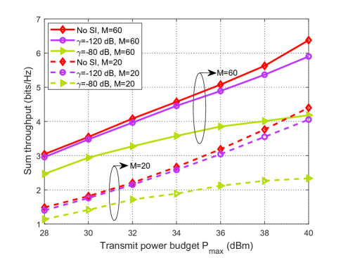
Figure 5: Sum throughput versus $P_{\max}$.

V-1 Effect of imperfect SIC

In Fig. 5, we study the sum throughput versus $P_{\max}$ for different values of $\gamma$ with $K=5$. It is observed that when $M=20$, the proposed scheme with $\gamma=-120~{}{\rm dB}$ achieves nearly the same sum throughput as that with perfect SIC when $P_{\max}\leq 34~{}{\rm dBm}$, even when $P_{\max}$ becomes large, i.e., $P_{\max}\geq 34~{}{\rm dBm}$, the performance gap between two schemes is still small. In addition, we observe that as $\gamma$ becomes larger, the sum throughput will be smaller. This is expected since a higher value of $\gamma$ incurs stronger SI on the HAP receiver side, which will degrade the system performance. Especially, when $\gamma=-80~{}{\rm dB}$ and $M=20$, the sum throughput increases slowly with $P_{\max}$, even remains unchanged when $P_{\max}\geq 38~{}{\rm dBm}$, which indicates the importance of canceling the SI at the HAP. Similar results are also observed for $M=80$.

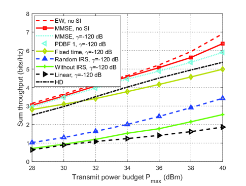
Figure 6: Sum throughput versus ${P}_{\rm max}$.

V-2 Sum Throughput Versus Transmit Power

In Fig. 6, we study the sum throughput obtained by all schemes versus $P_{\max}$ with $M=60$ and $K=5$. It can be observed that the EW-based approach achieves better performance than the MMSE-based approach in terms of sum throughput, which is consistent with the previous discussion. It is also observed that the sum throughput obtained by all schemes monotonically increases with $P_{\max}$, even with the imperfect SIC. This can be understood as follows. On the one hand, in the DL WET stage, i.e., $\tau_{0}$, the harvested energy by devices will significantly increase as $P_{\max}$ increases, which allows devices to transmit higher power for UL WIT. On the other hand, in the UL WIT stage, i.e., $\tau_{i},i\neq 0$, we can properly decrease the HAP transmit power to alleviate the SI at the HAP receiver side at the cost of transmitting less energy by devices, which is also able to provide some certain performance gains. In addition, we can observe that our proposed scheme outperforms the benchmark schemes with fixed time, with random IRS, and without IRS, especially as $P_{\max}$ increases, which demonstrates the benefits of the joint design of the IRS beamforming and resource allocation for improving the FD-WPCN system performance. As expected, we observe that our proposed FD-WPCN significantly outperforms the HD-WPCN, especially when the SI is perfectly cancelled. Moreover, it is observed that the scheme based on the linear EH model achieves less sum throughput compared to schemes based on the non-linear EH model due to the resource allocation mismatch. Furthermore, one can observe that the “PDBF 1” scheme achieves the same performance with our proposed scheme for the same $\gamma$, which indicates that the DBF for the dedicated DL WIT is not needed in practice (For $K=5$, the duration of DL WET is not zero, which has been discussed in Fig. 10). This is because although the harvested energy profiles for devices via dynamically adjusting the IRS phase-shift vector across each sub-slot is different from that via only optimizing one common IRS phase-shift vector over the entire DL WET duration, the impact incurred by this difference can be mitigated by optimizing the UL time allocation.

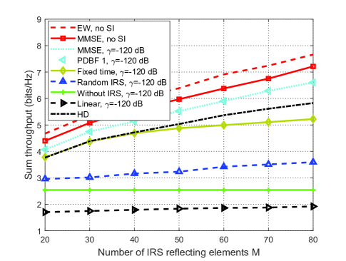
Figure 7: Sum throughput versus $M$.

V-3 Sum Throughput Versus Number of Reflecting Elements

In Fig. 7, we compare the sum throughput obtained by all schemes versus $M$ with $P_{\max}=40~{}{\rm dBm}$ and $K=5$. It is first observed that the sum throughput obtained by schemes with IRS phase shift optimization monotonically increases with $M$ since more reflecting elements installed at the IRS help achieve higher passive beamforming gain for both DL WET and UL WIT. We observe that the EW-based algorithm with perfect SIC outperforms the other schemes, which again demonstrates the superiority of the EW-based algorithm over the MMSE-based algorithm in terms of the sum throughput. In addition, we observe that with the same SI $\gamma=-120~{}{\rm dB}$, our proposed scheme achieves higher sum throughput than those schemes with fixed time, with random IRS, and without IRS, which demonstrates the benefits of the joint optimization of resource allocation and IRS phase shifts. Moreover, the proposed FD scheme outperforms the HD scheme in terms of sum throughput when the SI is well suppressed, i.e., $\gamma=-120~{}{\rm dB}$ or $\gamma=0$. Furthermore, the performance gap between two schemes would be more pronounced when $M$ becomes large. This is because installing more reflecting elements at the IRS will provide high passive beamforming gains and more energy will be harvested by devices under the FD mode than under the HD mode, which allows devices to transmit higher power for UL WIT.

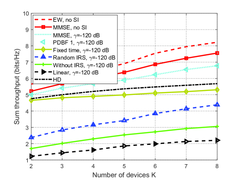
Figure 8: Sum throughput versus $K$.

V-4 Sum Throughput Versus Number of Devices

In Fig. 8, we compare the sum throughput obtained by all schemes versus $K$ with $P_{\max}=40~{}{\rm dBm}$ and $M=60$. It can be seen that the sum throughput obtained by all schemes increases as $K$ increases due to the more multiuser diversity and higher design flexibility of IRS. In addition, as $K$ increases, the performance gap between our proposed scheme and the fixed time scheme becomes larger. This can be understood as follows. Since some of devices have poor channel conditions, it is not wise to allocate the time to these devices. In contrast, with the optimization of time allocation, we may not assign any time to devices with poor channel conditions for UL WIT, while we assign more time to devices with good channel conditions for UL WIT. Therefore, the optimization of time allocation plays an important role in system design, especially when $K$ is large. Moreover, we can observe that our proposed scheme outperforms the other benchmark schemes, which again demonstrates the benefits of exploiting both IRS and FD in the MIMO WPCN. Furthermore, we can also observe that with $\gamma=-120~{}{\rm dB}$, the “PDBF 1” scheme achieves the same performance with our proposed scheme, which further demonstrates the non-necessity of adopting DBF for DL WET.

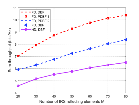
Figure 9: Sum throughput versus $M$ for three types of IRS configurations with $P_{\max}=40~{}{\rm dBm}$ and $K=15$.

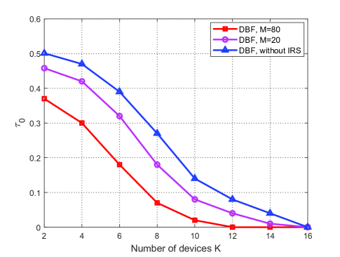
Figure 10: Duration of DL WET versus $K$ with $P_{\max}=40~{}{\rm dBm}$.

V-5 Dynamic versus Static IRS Beamforming

In Fig. 9, we study three types of IRS beamforming configurations in terms of sum throughout to strike a balance between the system performance and signaling overhead as well as implementation complexity. We compare the following schemes. 1) FD, DBF: Our proposed scheme; 2) FD, PDBF: There are two special cases for the PDBF scheme. For the first PDBF case, i.e., PDBF 1, which has been previously discussed. For the second PDBF case, i.e., PDBF 2, where there are two different IRS phase-shift vectors during the whole transmission period with one for DL WET and the other for UL WIT; 3) FD, SBF: This is the static IRS beamforming (SBF) scheme, where one common IRS phase-shift vector is applied for both DL WET and UL WIT. 4) HD, DBF: Compared to the “FD, DBF” scheme, the HAP operates in the HD mode. First, it is observed that the “FD, DBF” scheme achieves the same system performance with the “FD, PDBF 1” scheme. This is because as $K$ becomes large, i.e., $K=15$, the duration of DL WET time slot, i.e., $\tau_{0}$, becomes almost zero. To under it more clearly, we study the duration of DL WET time slot $\tau_{0}$ versus $K$ as shown in Fig. 10. It is observed that $\tau_{0}$ monotonically decreases as $K$ increases. This is because when $K$ is small, the number of time slots for EH during UL WIT is also small and thus the dedicated DL WET time slot plays an important role in improving system performance, while as $K$ becomes large, the number of time slots for UL WIT becomes large, which indicates that the devices can still harvest sufficient energy even without the dedicated DL WET time slot. Similar results can also be observed by comparing the “FD, PDBF 2” scheme with the “FD, SBF” scheme. In addition, we can observe that the “FD, DBF” scheme (or “FD, PDBF 1” scheme) significantly outperforms the “FD, PDBF 2” scheme (or “FD, SBF” scheme). This is expected since for the former, the IRS is able to proactively generate artificial time-varying channels over each time slot to adapt to UL WIT so as to improve the system performance.

VI Conclusion

In this paper, we studied the joint design of passive beamforming and resource allocation for the IRS-aided MIMO FD-WPCN by taking into account the finite SI and the non-linear EH model. Specifically, the DL/UL time allocation, precoding matrices, transmit covariance matrices, and phase shifts were jointly optimized to maximize the sum throughput of the IRS-aided MIMO FD-WPCN. We proposed two algorithms, namely EW-based algorithm and MMSE-based algorithm, to achieve a balance between the system performance and the computational complexity. Simulation results demonstrated the benefits of the IRS used for enhancing the performance of the MIMO FD-WPCN, especially when the DBF was adopted. Besides, the results revealed that the FD mode is more beneficial than the HD mode when the SI is effectively suppressed. Furthermore, the results also showed that the DBF for DL WET may not be necessary in practice. This work can be further extended by considering imperfect CSI, multiple IRSs, and quality-of-service constraints at devices, etc., which will be left as future work.

References

• [1] I. Krikidis, S. Timotheou, S. Nikolaou, G. Zheng, D. W. K. Ng, and R. Schober, “Simultaneous wireless information and power transfer in modern communication systems,” IEEE Commun. Mag., vol. 52, no. 11, pp. 104–110, Nov. 2014.
• [2] H. Ju and R. Zhang, “Throughput maximization in wireless powered communication networks,” IEEE Trans. Wireless Commun., vol. 13, no. 1, pp. 418–428, Jan. 2014.
• [3] H. Chingoska, Z. Hadzi-Velkov, I. Nikoloska, and N. Zlatanov, “Resource allocation in wireless powered communication networks with non-orthogonal multiple access,” IEEE Wireless Commun. Lett., vol. 5, no. 6, pp. 684–687, Dec. 2016.
• [4] Q. Wu, W. Chen, D. W. K. Ng, and R. Schober, “Spectral and energy-efficient wireless powered IoT networks: NOMA or TDMA?” IEEE Trans. Veh. Technol., vol. 67, no. 7, pp. 6663–6667, Jul. 2018.
• [5] H. Lee, K.-J. Lee, H.-B. Kong, and I. Lee, “Sum-rate maximization for multiuser MIMO wireless powered communication networks,” IEEE Trans. Veh. Technol., vol. 65, no. 11, pp. 9420–9424, Nov. 2016.
• [6] G. Yang, C. K. Ho, R. Zhang, and Y. L. Guan, “Throughput optimization for massive MIMO systems powered by wireless energy transfer,” IEEE J. Sel. Areas Commun., vol. 33, no. 8, pp. 1640–1650, Aug. 2015.
• [7] H. Ju and R. Zhang, “Optimal resource allocation in full-duplex wireless-powered communication network,” IEEE Trans. Commun., vol. 62, no. 10, pp. 3528–3540, Oct. 2014.
• [8] X. Kang, C. K. Ho, and S. Sun, “Full-duplex wireless-powered communication network with energy causality,” IEEE Trans. Wireless Commun., vol. 14, no. 10, pp. 5539–5551, Oct. 2015.
• [9] R. Rezaei, S. Sun, X. Kang, Y. L. Guan, and M. R. Pakravan, “Secrecy throughput maximization for full-duplex wireless powered IoT networks under fairness constraints,” IEEE Internet of Things J., vol. 6, no. 4, pp. 6964–6976, Aug. 2019.
• [10] B. K. Chalise, H. A. Suraweera, G. Zheng, and G. K. Karagiannidis, “Beamforming optimization for full-duplex wireless-powered MIMO systems,” IEEE Trans. Commun., vol. 65, no. 9, pp. 3750–3764, Sept. 2017.
• [11] Q. Wu, S. Zhang, B. Zheng, C. You, and R. Zhang, “Intelligent reflecting surface-aided wireless communications: A tutorial,” IEEE Trans. Commun., vol. 69, no. 5, pp. 3313–3351, May 2021.
• [12] M. Di Renzo et al., “Smart radio environments empowered by reconfigurable AI meta-surfaces: An idea whose time has come,” EURASIP J. Wireless Commun. Netw., vol. 2019, no. 1, pp. 1–20, May 2019.
• [13] Q. Wu and R. Zhang, “Towards smart and reconfigurable environment: Intelligent reflecting surface aided wireless network,” IEEE Commun. Mag., vol. 58, no. 1, pp. 106–112, Jan. 2020.
• [14] Q. Wu and R. Zhang, “Intelligent reflecting surface enhanced wireless network via joint active and passive beamforming,” IEEE Trans. Wireless Commun., vol. 18, no. 11, pp. 5394–5409, Nov. 2019.
• [15] X. Guan, Q. Wu, and R. Zhang, “Intelligent reflecting surface assisted secrecy communication: Is artificial noise helpful or not?” IEEE Wireless Commun. Lett., vol. 9, no. 6, pp. 778–782, Jun. 2020.
• [16] Z. Zhang, L. Lv, Q. Wu, H. Deng, and J. Chen, “Robust and secure communications in intelligent reflecting surface assisted NOMA networks,” IEEE Commun. Lett., 2020, early access, doi: 10.1109/LCOMM.2020.3039811.
• [17] X. Yu, D. Xu, Y. Sun, D. W. K. Ng, and R. Schober, “Robust and secure wireless communications via intelligent reflecting surfaces,” IEEE J. Sel. Areas Commun., vol. 38, no. 11, pp. 2637–2652, Nov. 2020.
• [18] C. Pan, H. Ren, K. Wang, W. Xu, M. Elkashlan, A. Nallanathan, and L. Hanzo, “Multicell MIMO communications relying on intelligent reflecting surfaces,” IEEE Trans. Wireless Commun., vol. 19, no. 8, pp. 5218–5233, Aug. 2020.
• [19] M. Hua, Q. Wu, D. W. K. Ng, J. Zhao, and L. Yang, “Intelligent reflecting surface-aided joint processing coordinated multipoint transmission,” IEEE Trans. Commun., 2020, early access, doi: 10.1109/TCOMM.2020.3042275.
• [20] H. Xie, J. Xu, and Y. F. Liu, “Max-min fairness in IRS-aided multi-cell MISO systems with joint transmit and reflective beamforming,” IEEE Trans. Wireless Commun., 2020, early access, doi: 10.1109/TWC.2020.3033332.
• [21] J. Zhu et al., “Power efficient IRS-assisted NOMA,” IEEE Trans. Commun., vol. 69, no. 2, pp. 900–913, Feb. 2021.
• [22] Z. Ding and H. Vincent Poor, “A simple design of IRS-NOMA transmission,” IEEE Commun. Lett., vol. 24, no. 5, pp. 1119–1123, May 2020.
• [23] G. Chen, Q. Wu, W. Chen, D. W. K. Ng, and L. Hanzo, “IRS-aided wireless powered MEC systems: TDMA or NOMA for computation offloading?” 2021. [Online]. Available: https://arxiv.org/abs/2108.06120.
• [24] Q. Wu and R. Zhang, “Weighted sum power maximization for intelligent reflecting surface aided SWIPT,” IEEE Wireless Commun. Lett., vol. 9, no. 5, pp. 586–590, May 2020.
• [25] C. Pan et al., “Intelligent reflecting surface enhanced MIMO broadcasting for simultaneous wireless information and power transfer,” IEEE J. Sel. Areas Commun., vol. 38, no. 8, pp. 1719–1734, Aug. 2020.
• [26] Z. Li, W. Chen, and Q. Wu, “Joint beamforming design and power splitting optimization in IRS-assisted SWIPT NOMA networks,” 2020. [Online]. Available: https://arxiv.org/abs/2011.14778.
• [27] S. Zargari, A. Khalili, Q. Wu, M. R. Mili, and D. W. K. Ng, “Max-min fair energy-efficient beamforming design for intelligent reflecting surface-aided SWIPT systems with non-linear energy harvesting model,” IEEE Trans. Veh. Technol., 2021, early access, doi: 10.1109/TVT.2021.3077477.
• [28] W. Tang et al., “Wireless communications with reconfigurable intelligent surface: Path loss modeling and experimental measurement,” IEEE Trans. Wireless Commun., vol. 20, no. 1, pp. 421–439, Jan. 2021.
• [29] Q. Wu et al., “IRS-aided WPCNs: A new optimization framework for dynamic IRS beamforming,” 2021. [Online]. Available: https://arxiv.org/abs/2107.03251.
• [30] Q. Wu, X. Guan, and R. Zhang, “Intelligent reflecting surface-aided wireless energy and information transmission: An overview,” Proceedings of the IEEE, 2021, early access, doi: 10.1109/JPROC.2021.3121790.
• [31] Q. Wu, X. Zhou, and R. Schober, “IRS-assisted wireless powered NOMA: Is dynamic passive beamforming really needed?” 2021. [Online]. Available: https://arxiv.org/abs/2102.08739.
• [32] B. Lyu, P. Ramezani, D. T. Hoang, S. Gong, Z. Yang, and A. Jamalipour, “Optimized energy and information relaying in self-sustainable IRS-empowered WPCN,” IEEE Trans. Commun., vol. 69, no. 1, pp. 619–633, Jan. 2021.
• [33] D. Zhang, Q. Wu, M. Cui, G. Zhang, and D. Niyato, “Throughput maximization for IRS-assisted wireless powered hybrid NOMA and TDMA,” IEEE Wireless Commun. Lett., 2021, early access, doi: 10.1109/LWC.2021.3087495.
• [34] S. Gong, C. Xing, S. Wang, L. Zhao, and J. An, “Throughput maximization for intelligent reflecting surface aided MIMO WPCNs with different DL/UL reflection patterns,” IEEE Trans. Signal Process., vol. 69, pp. 2706–2724, Apr. 2021.
• [35] Z. Chu, P. Xiao, D. Mi, W. Hao, M. Khalily, and L.-L. Yang, “A novel transmission policy for intelligent reflecting surface assisted wireless powered sensor networks,” 2021. [Online]. Available: https://arxiv.org/abs/2104.14000.
• [36] Y. Zheng, S. Bi, Y. J. Zhang, Z. Quan, and H. Wang, “Intelligent reflecting surface enhanced user cooperation in wireless powered communication networks,” IEEE Wireless Commun. Lett., vol. 9, no. 6, pp. 901–905, Jun. 2020.
• [37] B. Clerckx et al., “Fundamentals of wireless information and power transfer: From RF energy harvester models to signal and system designs,” IEEE J. Sel. Areas Commun., vol. 37, no. 1, pp. 4–33, Jan. 2019.
• [38] D. Xu, X. Yu, Y. Sun, D. W. K. Ng, and R. Schober, “Resource allocation for IRS-assisted full-duplex cognitive radio systems,” IEEE Trans. Commun., vol. 68, no. 12, pp. 7376–7394, Dec. 2020.
• [39] H. Shen, T. Ding, W. Xu, and C. Zhao, “Beamformig design with fast convergence for IRS-aided full-duplex communication,” IEEE Commun. Lett., vol. 24, no. 12, pp. 2849–2853, Dec. 2020.
• [40] Y. Cai, M.-M. Zhao, K. Xu, and R. Zhang, “Intelligent reflecting surface aided full-duplex communication: Passive beamforming and deployment design,” arXiv preprint arXiv:2012.07218, 2020.
• [41] M. Hua and Q. Wu, “Joint dynamic passive beamforming and resource allocation for IRS-aided full-duplex WPCN,” 2021. [Online]. Available: https://arxiv.org/abs/2108.06660.
• [42] J. Xu and R. Zhang, “Energy beamforming with one-bit feedback,” IEEE Trans. Signal Process., vol. 62, no. 20, pp. 5370–5381, Oct. 2014.
• [43] E. Boshkovska, D. W. K. Ng, N. Zlatanov, and R. Schober, “Practical non-linear energy harvesting model and resource allocation for SWIPT systems,” IEEE Commun. Lett., vol. 19, no. 12, pp. 2082–2085, Dec. 2015.
• [44] Y. Lu, K. Xiong, P. Fan, Z. Ding, Z. Zhong, and K. B. Letaief, “Global energy efficiency in secure MISO SWIPT systems with non-linear power-splitting EH model,” IEEE J. Sel. Areas Commun., vol. 37, no. 1, pp. 216–232, Jan. 2019.
• [45] S. Boyd and L. Vandenberghe, Convex Optimization.   Cambridge University Press, 2004.
• [46] A. Ben-Tal and A. Nemirovski, Lectures on modern convex optimization: analysis, algorithms, and engineering applications.   SIAM, 2001.
• [47] J. Gondzio and T. Terlaky, “A computational view of interior point methods,” Advances in linear and integer programming. Oxford Lecture Series in Mathematics and its Applications, vol. 4, pp. 103–144, 1996.
• [48] Q. Shi et al., “An iteratively weighted MMSE approach to distributed sum-utility maximization for a MIMO interfering broadcast channel,” IEEE Trans. Signal Process., vol. 59, no. 9, pp. 4331–4340, Sep. 2011.
• [49] M. S. Lobo, L. Vandenberghe, S. Boyd, and H. Lebret, “Applications of second-order cone programming,” Linear algebra and its applications, vol. 284, no. 1-3, pp. 193–228, Nov. 1998.
• [50] D. Nguyen, L.-N. Tran, P. Pirinen, and M. Latva-aho, “On the spectral efficiency of full-duplex small cell wireless systems,” IEEE Trans. Wireless Commun., vol. 13, no. 9, pp. 4896–4910, Sept. 2014.