Cao et al. Optimal Partition for Multi-Type Queueing System Optimal Partition for Multi-Type Queueing System

Shengyu Cao, Simai He School of Information Management and Engineering, Shanghai University of Finance and Economics, China, 200433, shengyu.cao@163.sufe.edu.cn, simaihe@mail.shufe.edu.cn Zizhuo Wang School of Data Science, The Chinese University of Hong Kong, Shenzhen, China, 518172, wangzizhuo@cuhk.edu.cn Yifan Feng Department of Analytics and Operations, NUS Business School, National University of Singapore, Singapore, 119245, yifan.feng@nus.edu.sg

We analyze the optimal partition and assignment strategy for an uncapacitated FCFS queueing system with multiple types of customers. Each type of customers is associated with a certain arrival and service rate. The decision maker can partition the server into sub-queues, each with a smaller service capacity, and can route different types of customers to different sub-queues (deterministically or randomly). The objective is to minimize the overall expected waiting time.

First, we show that by properly partitioning the queue, it is possible to reduce the expected waiting time of customers, and there exist a series of instances such that the reduction can be arbitrarily large. Then we consider four settings of this problem, depending on whether the partition is given (thus only assignment decision is to be made) or not and whether each type of customers can only be assigned to a unique queue or can be assigned to multiple queues in a probabilistic manner. When the partition is given, we show that this problem is NP-hard in general if each type of customers must be assigned to a unique queue. When the customers can be assigned to multiple queues in a probabilistic manner, we identify a structure of the optimal assignment and develop an efficient algorithm to find the optimal assignment. When the decision maker can also optimize the partition, we show that the optimal decision must be to segment customers deterministically based on their service rates, and to assign customers with consecutive service rates into the same queue. Efficient algorithms are also proposed in this case. Overall, our work is the first to comprehensively study the queue partition problem based on customer types, which has the potential to increase the efficiency of queueing system.

queue partitioning; multi-type queueing system This version:

1 Introduction and Literature Review

Queue is pervasive in daily activities. The analysis of queue pooling and partitioning has important ramifications in improving the performance of queueing system. Consequently, whether pooling the queue will reduce the average waiting time has been extensively studied in the literature under the contents of emergency departments (see, e.g., Saghafian et al. 2012), call centers (see, e.g., Jouini et al. 2008), computer server farms (see, e.g., Harchol-Balter et al. 2009), etc. A classical conclusion is that when customer service time distributions are homogeneous, a pooled queue is always more appealing (Smith and Whitt 1981). Otherwise, dedicated queues can outperform in some cases (Whitt 1999). Indeed, separating arrivals to different queues according to expected service time is ubiquitous in practice, including express lines in supermarkets, fast track in emergency departments, and size interval task assignment (SITA) policy employed in computer server farms. Notwithstanding its prevalent use, very few results rigorously discuss how to make an optimal partition of queues based on the expected service time. Such insufficient study of queue partitioning, owing primarily to the difficulty of analysis, motivates this work.

In this paper, we consider a service system with several types of customers, each with exponential arrival and service time. We consider the scenario where a single server can be partitioned to multiple servers with different serving capacities, and each type of customers can be assigned to one of the partitions (or assigned to several partitions with certain probabilities). In our work, we are concerned with the expected waiting time of all customers. We aim to answer the following questions in our paper.

1. Whether partitioning the server can lead to a smaller expected waiting time?

2. If the partition of the servers is given, what is the optimal way to assign each type of customers?

3. If the partition of the servers can be adjusted, what is the optimal way to partition the server and to assign each type of customers?

To answer these questions, we build a queueing model with two sets of decisions. One is how to allocate the server resources (we call the partition decision); the other is how to assign each type of customers (we call the assignment decision). First, we show that by properly partitioning the queue and making proper assignment, it is possible to reduce the expected total waiting time of customers, and the gap between not partitioning versus the optimal partition and assignment could be arbitrarily large. Then we consider four settings of this problem, depending on whether the partition is given (thus only assignment decision is to be made) or not and whether each type of customers can only be assigned to a unique queue or can be assigned to multiple queues in a probabilistic manner. When the partition of the servers is given and customers of the same type have to be assigned to a single server, we show that the problem is NP-hard even when there are only two servers. When customers of the same type can be assigned to multiple servers in a probabilistic manner, efficient algorithms are provided to compute the optimal assignment. Specifically, when there are two servers with given serving capacity and customers can be assigned to each server with certain probability, the optimal assignment contains at most three continuous segments ranked by the customers’ service rate. Interestingly, we find that it is possible that customers in the first and third segments are assigned to one server, while customers in the second segment are assigned to the other server. When both partition and assignment can be optimized, we show that even when assignment with probabilities is allowed, customers of the same type will be assigned to the same server under the optimal assignment. Moreover, we can always find an optimal solution by partitioning customers into sub-intervals based on their service rates, where customers within the same sub-interval are assigned to the same server. To summarize, our work provides a comprehensive analysis of the queue partition problem based on customer type. We identify the computational complexity, the solution structure, and propose algorithms for each case of the problem. We believe that our result can help decision maker design more efficient queueing system in practice.

In the remainder of this section, we review some related work. Our work is closely related to the literature that studies queue partitions under various settings. Among these studies, one stream considers the queue partition problem where the partition is done according to the job size. In particular, they assume that upon arrival the service time is known. Based on the known service time, task assignment decision is then made. Under such assumption, a class of policy called the size interval task assignment (SITA) policy is proposed. A seminal result in this stream is by Harchol-Balter et al. (2009), who state that when traffic is heavy and job-size distributions have high variability, the SITA policy outperforms the policy that assigns incoming jobs to the queue with least total job size remaining, which is called the Least-Work-Left (LWL) policy. Such partition based on the actual job size is reasonable for deterministic computer workloads. However, in fields of emergency departments, call centers, and cloud computing system with general tasks (e.g. machine learning or optimization tasks), service time is often unknown before the service is completed. Instead, it is common that we only have the type information, i.e., only the distribution of service time is known upon customers’ arrival. In this paper, we assume the type information is known but the actual service time is unknown, and study the partition problem under this setting.

In the queueing literature, there are two types of models characterizing how the service can be pooled or partitioned. In the first type of model, the decision maker determines the number of servers assigned to each sub-queue (see, e.g., Hu and Benjaafar 2009, Hung and Posner 2007, Whitt 1999), while in the second type of model, the decision maker decides the service rate assigned to each sub-queue (see, e.g., Hassin et al. 2015, Yu et al. 2015, Allon and Federgruen 2008). When pooling service rates, two single-server queues are merged into a new single-server queue, where service rates are aggregated (see, e.g., Andradóttir et al. 2017, Iyer and Jain 2004, Mandelbaum and Reiman 1998, Kleinrock 1976). Mandelbaum and Reiman (1998) point out that when traffic is heavy, the performance of pooling service rates coincides that of pooling servers. Our work adopts the second model and assumes that the service rates can be pooled or partitioned.

Recently, researchers analyze the effect of pooling under more sophisticated settings. For instance, Argon and Ziya (2009) discuss how imperfect classification influences the decision process of partitioning. Sunar et al. (2021) analyze the case where customers are delay-sensitive and discuss the benefit of pooling. Cao et al. (2020) argue that with a proper routing policy, idle time of servers in dedicate systems can be reduced. In another work, Hu and Benjaafar (2009) study how to partition the queueing systems during rush hour, where a plethora of customer arrivals occur in a short time window and few or even no customers appear thereafter. They assume instant arrival of customers and use single-queue formula to analyze the best partition decision. They prove that separating each customer type is optimal, and give the optimal allocation of servers to each customer type. In contrast with this work, we consider the optimal partition in a stationary environment. Also, we assume the server capacity is divisible. Our goal is to analyze whether a subset of customer types should be pooled and how many server resources should be assigned to this group of customer types. The work that is closest to ours is Whitt (1999). In this work, the author points out that if the queues are pooled, the economies of scale will increase the service resource utilization and minimize the idle time of the server. However, when the variation of the service time distributions is very large, separating fast customers from the others may save them from being blocked and offset the lower utilization disadvantage, thus increasing the overall efficiency. Whitt (1999) considers when and how to partition a pool of identical indivisible servers into sub-groups to minimize the overall number of servers required to meet the underlying requirement on system delay. However, the analysis is based on a heuristic method and it does not analyze the structure of the optimal partition. We complement this work and establish the optimal structure of customer assignment by rigorously quantifying the trade-off between servers being under-utilized and fast jobs getting blocked by slow jobs.

The rest of the paper is organized as follows. We first formulate a queue partition problem with two sub-queues in Section 2, and continue with our main results in Section 3. In Section 4, we extend our results to multiple queues. Finally, we summarize our results in Section 5.

2 Model of Two Queues

We consider a queueing system with $n$ types of customers. Type $i$ customers arrive at the system according to a Poisson process with an arrival rate $\lambda_{i}$ and have an exponential service time distribution with average service time $\frac{1}{\mu_{i}}$ under a unit server. We assume the total serving capacity is $1$ and the serving capacity is divisible, meaning that it can be divided into several queues. In our base model, we consider the case where the serving capacity can be divided into two queues, each with serving capacity $\alpha$ and $1-\alpha$ respectively. When a server with capacity $\alpha$ serves the $i$th type of customers, the service time distribution becomes exponential with average service time $\frac{1}{\alpha\mu_{i}}$. In the following, we consider the problem of dividing the service capacity and assigning customers to each sub-queue with their type information only. Our objective is to minimize the expected total waiting time of all customers in the queueing system.

We consider two types of problems. In the first type of problem, we assume the partition $\alpha$ is given, and we are interested in finding the optimal assignment of each type of customers. In the second type of problem, we jointly decide the partition $\alpha$ and the assignment of each type of customers.

For each aforementioned problem, we consider two types of assignment policies: a deterministic policy and a stochastic policy. Under the deterministic policy, each type of customers can only be assigned to a unique queue. Specifically, in this case, we use $\boldsymbol{x}\in\left\{0,1\right\}^{n}$ to indicate the assignment of each type of customers, where $x_{i}=1$ ($x_{i}=0$, respectively) denotes that the $i$th type of customers is assigned to the first queue (second queue, respectively). In contrast, under the stochastic policy, customers of the same type can be assigned to both queues each with certain probabilities. Specifically, in this case, we use $\boldsymbol{x}\in[0,1]^{n}$ to indicate the assignment of each type of customers, where $x_{i}$ denotes the probability of the $i$th type of customers assigned to the first queue. By Pollaczek–Khinchine formula, given partition $\alpha$ and assignment $\boldsymbol{x}$, the expected waiting time can be calculated as

$$f(\boldsymbol{x},\alpha):=\frac{\sum_{i=1}^{n}\frac{\lambda_{i}x_{i}}{\mu_{i}^{2}}}{\alpha^{2}-\alpha\sum_{i=1}^{n}\frac{\lambda_{i}x_{i}}{\mu_{i}}}\cdot\frac{\sum_{i=1}^{n}x_{i}\lambda_{i}}{\sum_{i=1}^{n}\lambda_{i}}+\frac{\sum_{i=1}^{n}\frac{\lambda_{i}(1-x_{i})}{\mu_{i}^{2}}}{(1-\alpha)^{2}-(1-\alpha)\sum_{i=1}^{n}\frac{\lambda_{i}(1-x_{i})}{\mu_{i}}}\cdot\frac{\sum_{i=1}^{n}(1-x_{i})\lambda_{i}}{\sum_{i=1}^{n}\lambda_{i}},$$

if $0<\alpha<1$ and $f(\boldsymbol{x},\alpha)=\frac{\sum_{i=1}^{n}\frac{\lambda_{i}}{\mu_{i}^{2}}}{1-\sum_{i=1}^{n}\frac{\lambda_{i}}{\mu_{i}}}$ if $\alpha=0,\boldsymbol{x}=\boldsymbol{0}$ or $\alpha=1,\boldsymbol{x}=\boldsymbol{1}$, where $\boldsymbol{0}$ ($\boldsymbol{1}$, respectively) is an all-$0$ (all-$1$, respectively) vector. Note that for $f(\boldsymbol{x},\alpha)$ to be meaningful, we must have

$$(\boldsymbol{x},\alpha)\in\mathcal{F}=\left\{(\boldsymbol{x},\alpha):\sum_{i=1}^{n}\frac{\lambda_{i}x_{i}}{\mu_{i}}<\alpha<\sum_{i=1}^{n}\frac{\lambda_{i}x_{i}}{\mu_{i}}+1-\sum_{i=1}^{n}\frac{\lambda_{i}}{\mu_{i}}\right\}\bigcup\left\{(\boldsymbol{0},0),(\boldsymbol{1},1)\right\},$$

or equivalently, $\boldsymbol{x}\in\mathcal{F}_{\alpha}$ where

$$\mathcal{F}_{\alpha}=\left\{\boldsymbol{x}:\sum_{i=1}^{n}\frac{\lambda_{i}x_{i}}{\mu_{i}}<\alpha<\sum_{i=1}^{n}\frac{\lambda_{i}x_{i}}{\mu_{i}}+1-\sum_{i=1}^{n}\frac{\lambda_{i}}{\mu_{i}}\right\},$$

if $0<\alpha<1$ and $\mathcal{F}_{0}=\left\{\boldsymbol{0}\right\},\mathcal{F}_{1}=\left\{\boldsymbol{1}\right\}$.

Classified by the type of problem (assignment only versus partition and assignment) and the type of policy considered (deterministic versus stochastic), we are interested in solving the following four problems:

• The deterministic assignment problem for given $\alpha$:

  $$\textup{(DAP)}\quad\inf_{\boldsymbol{x}} \quad f(\boldsymbol{x},\alpha)$$

  s.t. $$\quad\boldsymbol{x}\in\mathcal{F}_{\alpha};\quad x_{i}\in\left\{0,1\right\},\;i=1,\dots,n.$$ (1)

• The stochastic assignment problem for given $\alpha$:

  $$\textup{(SAP)}\quad\inf_{\boldsymbol{x}} \quad f(\boldsymbol{x},\alpha)$$

  s.t. $$\quad\boldsymbol{x}\in\mathcal{F}_{\alpha};\quad x_{i}\in[0,1],\;i=1,\dots,n.$$ (2)

• The deterministic partition problem:

  $$\textup{(DPP)}\quad\inf_{\boldsymbol{x},\alpha} \quad f(\boldsymbol{x},\alpha)$$

  s.t. $$\quad(\boldsymbol{x},\alpha)\in\mathcal{F};$$ (3)

  $$\quad 0\leq\alpha\leq 1;\quad x_{i}\in\left\{0,1\right\},\;i=1,\dots,n.$$

• The stochastic partition problem:

  $$\textup{(SPP)}\quad\inf_{\boldsymbol{x},\alpha} \quad f(\boldsymbol{x},\alpha)$$

  s.t. $$\quad(\boldsymbol{x},\alpha)\in\mathcal{F};$$ (4)

  $$\quad 0\leq\alpha\leq 1;\quad x_{i}\in[0,1],\;i=1,\dots,n.$$

Before we proceed, we show that in general, by making proper partitioning and assignment, one can reduce the expected waiting time. Moreover, the improvement can be arbitrarily large. We have the following proposition.

Proposition 2.1

For any $\epsilon>0$, there exist input parameters $\{\lambda_{i}\}_{i=1}^{n},\{\mu_{i}\}_{i=1}^{n}$ and $\boldsymbol{x},\alpha$ such that $f(\boldsymbol{x},\alpha)<\epsilon f(\boldsymbol{0},0)$.

To illustrate, consider two types of customers with $\lambda_{1}=t,\lambda_{2}=\mu_{1}=1,\mu_{2}=\frac{1}{t^{3}}$ where $0<t\leq\frac{1}{4}$. For partition $\alpha=1-t$ and assignment $x_{1}=1,x_{2}=0$, we have $f(\boldsymbol{x},\alpha)=\left(\frac{t^{2}}{1-2t}+\frac{t^{4}}{1+t}\right)\frac{1}{1-t^{2}},f(\boldsymbol{0},0)=\frac{t+t^{6}}{1-t-t^{3}}$, thus

$$\lim_{t\to 0}\frac{f(\boldsymbol{x},\alpha)}{f(\boldsymbol{0},0)}=0.$$

The intuition is that when a plethora of customers who can be served quickly are blocked by some slow minority, a huge reduction to the average waiting time can be obtained by allocating some dedicate resource for the fast majority. Therefore, partitioning the queue can make a significant improvement in the overall efficiency in this case.

We note that in Whitt (1999), the author also shows that by properly partitioning the queue, it is possible to reduce the total average waiting time. (The model in Whitt 1999 considers the split of servers, while in this paper, we consider the split of service capacity. Therefore, our model can be viewed as allowing more general partition than the one in Whitt 1999.) In Proposition 2.1, we further show that the improvement can be arbitrarily large under certain instances. This also implies that there does not exist a constant bound for the waiting time between the optimal split and a pooled server.

In subsequent sections, we will analyze the above-described problems. Particularly, we will analyze the computational complexity of the four problems and propose efficient algorithms.

3 Analysis and Main Results

In this section, we analyze the problems introduced in Section 2. Since $f(\boldsymbol{x},\alpha)=f(\boldsymbol{1}-\boldsymbol{x},1-\alpha)$, without loss of generality, we assume $\alpha\geq\frac{1}{2}$.

First, we have the following lemma which will be helpful for our subsequent analysis.

Lemma 3.1

For $(\boldsymbol{x},\alpha)\in\mathcal{F}$ and $x_{i}\geq 0$, $i=1,\dots,n$, $f(\boldsymbol{x},\alpha)$ is convex in $\alpha$ and is convex in $x_{i}$ for $i=1,\dots,n$.

The proof of Lemma 3.1 is by directly analyzing the second-order derivative of $f(\boldsymbol{x},\alpha)$ and thus is omitted. Despite Lemma 3.1, we note that $f(\boldsymbol{x},\alpha)$ is not jointly convex in $\boldsymbol{x}$ and $\alpha$ (it is not jointly convex in $\boldsymbol{x}$ either). Therefore, directly minimizing $f(\boldsymbol{x},\alpha)$ may be challenging. In the following, we analyze each case separately. We first study the DAP in (• ‣ 2). We have the following result.

Theorem 3.2

The DAP is NP-hard.

In the proof of Theorem 3.2, we reduce the well-known NP-hard problem, the Set Partition problem (see Garey and Johnson 1979) to the DAP. The detailed proof is referred to the Appendix.

Next we consider the SAP in (• ‣ 2). In the following discussion, without loss of generality, we assume $\mu_{i}\neq\mu_{j}$, for all $i,j$. If $\mu_{i}=\mu_{j}$, then we can redefine a type of customers with arrival rate $\lambda_{i}+\lambda_{j}$ and service rate $\mu_{i}$, to replace type $i$ and $j$ customers. It turns out that the optimal solution to this problem has a special structure. We describe it in the following theorem.

Theorem 3.3

Suppose $\lambda_{1},\dots,\lambda_{n},\mu_{1}>\cdots>\mu_{n}$ and $\alpha\geq\frac{1}{2}$ are given. For any optimal solution $\boldsymbol{x}^{*}$ to the SAP, there exist $0\leq l<h\leq n$ such that when $l<i<h$, $x^{*}_{i}=0$ and when $i>h$ or $i<l$, $x^{*}_{i}=1$. Moreover, the set $\mathcal{M}^{*}=\left\{i:0<x^{*}_{i}<1\right\}$ is either empty or singleton.

Theorem 3.3 states that the optimal solution to (• ‣ 2) can have at most three continuous segments, ranked by the service rate, in which the values in the first and third segments are $1$’s while the values in the second segment are strictly less than one. Moreover, in the second segment, at most one element (either the first or the last in this segment) can be fractional while all the other elements must be $0$. Also, we note that $l$ could be $0$, in which case the first segment does not exist. Similarly, $h$ could be $n$, in which case the third segment does not exist. When $l=0$ and $h=n$, only the second segment exists.

Now we give some more explanations on Theorem 3.3. If we refer to allowing assignment of all customer types to be fractional as full flexibility, and refer to allowing only one customer type’s assignment to be fractional as restricted flexibility, then Theorem 3.3 shows that restricted flexibility can bring as much benefit as full flexibility. Such a relation gives rise to an efficient algorithm to solve the SAP. Specifically, by Proposition 3.1, we know $f(\boldsymbol{x},\alpha)$ is convex in $x_{i}$ for all $i$. Thereby, an optimal solution to the SAP can be found by first enumerating all possible $0$ or $1$ elements in the solution (by Theorem 3.3 there are $\mathcal{O}(n^{2})$ of possible candidates), and then for each candidate solving a single-variable convex optimization for the fractional element (if exists). The detail of the algorithm is given in Algorithm 1.

Algorithm 1 Algorithm for Solving SAP

1:$\alpha\geq\frac{1}{2},\lambda_{i},\mu_{i},i=1,\dots,n$ and $\mu_{1}>\mu_{2}>\cdots>\mu_{n}$

2:$\boldsymbol{x}^{*}\in\mathbb{R}^{n}$

3:Initialize $f^{*}\leftarrow+\infty$

4:for $i=0,1,2,\dots,n$ do

5:     for $j=i+1,\dots,n+1$ do

6:         $x_{k}\leftarrow\begin{cases}0&\text{if }i<k<j\\ 1&\text{if }k>j\text{ or }k<i\\ \end{cases}$

7:         $x_{i}\leftarrow 0$, solve for optimal $x_{j}$

8:         Compute objective function value $f$ ($f\leftarrow+\infty$ if infeasible)

9:         if $f<f^{*}$ then

10:              $f^{*}\leftarrow f,\boldsymbol{x}^{*}\leftarrow\boldsymbol{x}$

11:         end if

12:         For $x_{j}=0,1$, solve for optimal $x_{i}$, repeat line 6 to line 9

13:     end for

14:end for

According to Theorem 3.3, it is possible that there exists a fractional component in the optimal solution. Also it is possible that the customers with the largest and the smallest service rate are assigned to the same queue, while the customers with intermediate service rate are assigned to the other queue. We illustrate such a case in the following example.

Consider three types of customers with $\lambda_{1}=0.4,\lambda_{2}=8,\lambda_{3}=0.2,\mu_{1}=16,\mu_{2}=12,\mu_{3}=10$. For partition $\alpha=0.8$, since $1-\alpha<\frac{\lambda_{2}}{\mu_{2}}$, we can see that $x_{2}=0$ is not feasible. Therefore, by Theorem 3.3 we know that the optimal solution must be in the form of $(x_{1},1,1)$, $(1,1,x_{3})$, $(0,x_{2},1)$, $(1,x_{2},0)$ or $(1,x_{2},1)$. According to the convexity of $f(\boldsymbol{x},\alpha)$ in $\boldsymbol{x}$, $\frac{\partial}{\partial x_{1}}f\left((x_{1},1,1),0.8\right)\geq\frac{\partial}{\partial x_{1}}f\left((x_{1},1,1),0.8\right)\biggr{\rvert}_{x_{1}=0}=0.18>0$, thereby the minimum of $(x_{1},1,1)$ type of solution is obtained at $f\left((0,1,1),0.8\right)=0.61$. Similarly, $\frac{\partial}{\partial x_{3}}f\left((1,1,x_{3}),0.8\right)\geq\frac{\partial}{\partial x_{3}}f\left((1,1,x_{3}),0.8\right)\biggr{\rvert}_{x_{3}=0}=0.15>0$, thereby the minimum of $(1,1,x_{3})$ type of solution is obtained at $f\left((1,1,0),0.8\right)=0.65$. Since $f\left((1,0.8,1),0.8\right)=0.37$, we can see that the optimal assignment cannot be in the form of $(x_{1},1,1)$ or $(1,1,x_{3})$. Therefore, the optimal solution must be of form $(0,x_{2},1)$, $(1,x_{2},0)$ or $(1,x_{2},1)$. Figure 1 shows how the values of $f\left((0,0.87+0.001\times\epsilon,1),0.8\right)$, $f\left((1,0.86+0.001\times\epsilon,0),0.8\right)$ and $f\left((1,0.83+0.001\times\epsilon,1),0.8\right)$ change with $\epsilon\in[0,10]$. By Lemma 3.1, $f$ is convex in $x_{2}$ given $x_{1}$ and $x_{3}$. Therefore, the result in Figure 1 indicates that the optimal value is in the form of $(1,x_{2},1)$. By Algorithm 1, we can calculate that the optimal solution is $\boldsymbol{x}^{*}=(1,0.836,1)$. Under this assignment, all of type $1$ and type $3$ and part of type $2$ customers are assigned to the first queue, and the rest of type $2$ customers are assigned to the second queue.$\hfill\square$

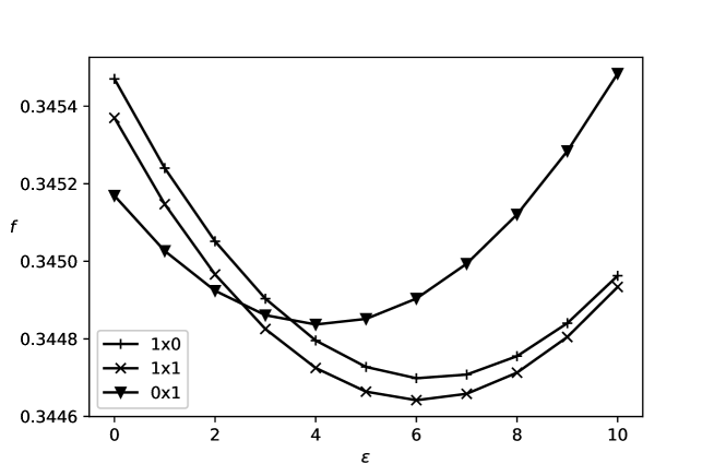
Figure 1: Objective function value under the assignment in the form of $(0,x_{2},1),(1,x_{2},0)$ and $(1,x_{2},1)$.

Now we have studied the queue assignment problem. We showed that the complexity of finding the optimal stochastic policy and the optimal deterministic policy are different. Next we consider the queue partition problem. We show that somewhat surprisingly, the deterministic partition problem (DPP) is equivalent to the stochastic partition problem (SPP). Furthermore, we show that both can be solved efficiently.

By analyzing properties of the optimal solution to the SPP, we have the following result.

Theorem 3.4

Given $\lambda_{i},i=1,2,\dots,n$ and $\mu_{1}>\mu_{2}>\cdots>\mu_{n}$. For any optimal solution $(\boldsymbol{x}^{*},\alpha^{*})$ to the SPP, there exists $i^{*}$ such that either $x^{*}_{i}=\begin{cases}1&\text{if }i\leq i^{*}\\ 0&\text{if }i>i^{*}\end{cases}$ or $x^{*}_{i}=\begin{cases}0&\text{if }i\leq i^{*}\\ 1&\text{if }i>i^{*}\end{cases}$.

Theorem 3.4 has several implications. First it indicates that the DPP is equivalent to the SPP, which also means that the additional flexibility of allowing fractional assignment does not have extra value in the queue partition problem. This is different from the queue assignment problem in which allowing fractional assignment may further reduce the expected waiting time compared to the optimal deterministic assignment. Second, the optimal partition in the SPP can only have two continuous segments, in which all customers with high service rates are assigned to one queue, and all the rest of customers are assigned to the other queue. Note that it is possible that one segment is empty (equivalently, $i^{*}=0$ or $n$), in which case the optimal partition is to choose $\alpha=1$ and assign all customers to one queue, and there is no benefit of splitting the queue.

With Theorem 3.4, we can design an efficient algorithm to solve the SPP (thus also solve the DPP). By Lemma 3.1, we know that given $\boldsymbol{x}$, $f(\boldsymbol{x},\alpha)$ is convex in $\alpha$. Therefore, the algorithm enumerates over all candidates of $\boldsymbol{x}$ (at most $n$ of them) and for each $\boldsymbol{x}$ solves a single-variable convex optimization for the optimal $\alpha$. The detailed algorithm is given in Algorithm 2.

Algorithm 2 Algorithm for Solving DPP and SPP

1:$\lambda_{i},i=1,\dots,n$ and $\mu_{1}>\mu_{2}>\cdots>\mu_{n}$

2:$\boldsymbol{x}^{*}\in\mathbb{R}^{n},\alpha^{*}\in\mathbb{R}$

3:Initialize $f^{*}\leftarrow+\infty$

4:for $i=1,2,\dots,n+1$ do

5:     $x_{k}=\begin{cases}0&\text{if }k<i\\ 1&\text{if }k\geq i\\ \end{cases}$

6:     $f\leftarrow\min_{\alpha}f(\boldsymbol{x},\alpha)$, $\bar{\alpha}\leftarrow\arg\min_{\alpha}f(\boldsymbol{x},\alpha)$

7:     if $f<f^{*}$ then

8:         $f^{*}\leftarrow f,\boldsymbol{x}^{*}\leftarrow\boldsymbol{x},\alpha^{*}\leftarrow\bar{\alpha}$

9:     end if

10:end for

4 Extension to Multiple Queues

In this section, we consider an extension of the base model in which the serving capacity can be divided into $k>2$ queues. We use $\boldsymbol{\alpha}\in[0,1]^{k}$ to represent the partition, where $\alpha_{j}$ denotes the allocated serving capacity of the $j$th queue. We also define $R(\boldsymbol{\alpha})=\{j:\alpha_{j}>0\}$. Under the stochastic policy, we use $X\in[0,1]^{n\times k}$ to denote the assignment of each type of customers, where $X_{ij}$ indicates the probability of the $i$th type of customers assigned to the $j$th queue. Under the deterministic policy, we use $X\in\left\{0,1\right\}^{n\times k}$ to denote the assignment of each type of customers, where $X_{ij}=1$ denotes that the $i$th type of customers is assigned to the $j$th queue. By Pollaczek–Khinchine formula, given partition $\boldsymbol{\alpha}$ and assignment $X$, the expected waiting time can be calculated as

$$f(X,\boldsymbol{\alpha}):=\sum_{j\in R(\boldsymbol{\alpha})}\left(\frac{\sum_{i=1}^{n}\frac{\lambda_{i}X_{ij}}{\mu_{i}^{2}}}{\alpha_{j}^{2}-\alpha_{j}\sum_{i=1}^{n}\frac{\lambda_{i}X_{ij}}{\mu_{i}}}\cdot\frac{\sum_{i=1}^{n}X_{ij}\lambda_{i}}{\sum_{i=1}^{n}\lambda_{i}}\right).$$

Note that for $f(X,\boldsymbol{\alpha})$ to be meaningful, we must have

$$(X,\boldsymbol{\alpha})\in\mathcal{F}=\left\{(X,\boldsymbol{\alpha}):\alpha_{j}>\sum_{i=1}^{n}\frac{\lambda_{i}X_{ij}}{\mu_{i}},\text{ for }j\in R(\boldsymbol{\alpha})\right\},$$

or equivalently,

$$X\in\mathcal{F}_{\boldsymbol{\alpha}}=\left\{X:\alpha_{j}>\sum_{i=1}^{n}\frac{\lambda_{i}X_{ij}}{\mu_{i}},\text{ for }j\in R(\boldsymbol{\alpha})\right\}.$$

Similarly, classified by the type of problem (assignment only versus partition and assignment) and the type of policy considered (deterministic versus stochastic), we are interested in solving the following four problems:

• The multi-queue deterministic assignment problem for given $\boldsymbol{\alpha}$:

  $$\textup{(}k\textup{-DAP)}\quad\inf_{X} \quad f(X,\boldsymbol{\alpha})$$

  s.t. $$\quad X\in\mathcal{F}_{\boldsymbol{\alpha}};$$ (5)

  $$\quad\sum_{j=1}^{k}X_{ij}=1,\quad i=1,\dots,n;$$

  $$\quad X_{ij}\in\left\{0,1\right\},\quad i=1,\dots,n,\;j=1,\dots,k.$$

• The multi-queue stochastic assignment problem for given $\boldsymbol{\alpha}$:

  $$\textup{(}k\textup{-SAP)}\quad\inf_{X} \quad f(X,\boldsymbol{\alpha})$$

  s.t. $$\quad X\in\mathcal{F}_{\boldsymbol{\alpha}};$$ (6)

  $$\quad\sum_{j=1}^{k}X_{ij}=1,\quad i=1,\dots,n;$$

  $$\quad X_{ij}\in[0,1],\quad i=1,\dots,n,\;j=1,\dots,k.$$

• The multi-queue deterministic partition problem:

  $$\textup{(}k\textup{-DPP)}\quad\inf_{X,\boldsymbol{\alpha}} \quad f(X,\boldsymbol{\alpha})$$

  s.t. $$\quad(X,\boldsymbol{\alpha})\in\mathcal{F};$$ (7)

  $$\quad\sum_{j=1}^{k}\alpha_{j}=1;\qquad\alpha_{j}\geq 0,\quad j=1,\dots,k;$$

  $$\quad\sum_{j=1}^{k}X_{ij}=1,\quad i=1,\dots,n;$$

  $$\quad X_{ij}\in\left\{0,1\right\},\quad i=1,\dots,n,\;j=1,\dots,k.$$

• The multi-queue stochastic partition problem:

  $$\textup{(}k\textup{-SPP)}\quad\inf_{X,\boldsymbol{\alpha}} \quad f(X,\boldsymbol{\alpha})$$

  s.t. $$\quad(X,\boldsymbol{\alpha})\in\mathcal{F};$$ (8)

  $$\quad\sum_{j=1}^{k}\alpha_{j}=1;\qquad\alpha_{j}\geq 0,\quad j=1,\dots,k;$$

  $$\quad\sum_{j=1}^{k}X_{ij}=1,\quad i=1,\dots,n;$$

  $$\quad X_{ij}\in[0,1],\quad i=1,\dots,n,\;j=1,\dots,k.$$

In the following analysis, we treat $k$ as a given constant. The result is stated in the following theorem.

Theorem 4.1

For any given $k$, we have the following results.

• The $k$-DAP is NP-hard.

• Suppose $\lambda_{1},\dots,\lambda_{n},\mu_{1}>\cdots>\mu_{n}$ and $\alpha_{1}\geq\cdots\geq\alpha_{k}>0$ are given. For any optimal solution $X^{*}$ to the $k$-SAP, there exist $0=l_{0}\leq l_{1}\leq l_{2}\leq\cdots\leq l_{2k-2}\leq l_{2k-1}=n+1$ and $o_{1},o_{2},\dots,o_{2k-1}\in\{1,2,\dots,k\}$ such that for each $1\leq h\leq 2k-1$, when $l_{h-1}<i<l_{h}$, $X^{*}_{i,o_{h}}=1$. Moreover, for $j=1,\dots,k$, the set $\mathcal{M}_{j}^{*}=\left\{i:0<X^{*}_{ij}<1\right\}$ is either empty or singleton.

• Given $\lambda_{i},i=1,2,\dots,n$ and $\mu_{1}>\mu_{2}>\cdots>\mu_{n}$. If the feasible set of the $k$-SPP is non-empty, then there exist an optimal solution $(X^{*},\boldsymbol{\alpha}^{*})$ to the $k$-SPP and $1=i_{0}\leq i_{1}\leq i_{2}\leq\cdots\leq i_{k-1}\leq i_{k}=n+1$ such that $X^{*}_{ij}=\begin{cases}1&\text{if }i_{j-1}\leq i<i_{j}\\ 0&\text{otherwise}\end{cases}$ for $j=1,2,\dots,k$.

Now we provide some explanations for Theorem 4.1. The first part of Theorem 4.1 is a simple extension of Theorem 3.2. The second part of Theorem 4.1 reveals a special column-wise property of the optimal $k$-SAP solution. Specifically, let $X^{*}\in\mathbb{R}^{n\times k}$ be an optimal solution to the $k$-SAP. Then each column of $X^{*}$ contains at most one fractional element. Moreover, for each column, if we call consecutive $1$’s as a block, then $X^{*}$ contains at most $2k-1$ blocks. To illustrate, consider a $k$-SAP problem with $n=5$ and $k=3$. As is shown in Figure 2, $X_{1}$ is a valid candidate of the optimal solution because the number of blocks is $5\leq 2k-1=5$, while $X_{2}$ is not because the number of blocks is $6>2k-1=5$. In particular, when $k=2$, the second statement in Theorem 4.1 reduces to the structure in Theorem 3.3.

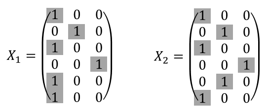
Figure 2: There are 5 blocks in $X_{1}$ and 6 blocks in $X_{2}$, where blocks are marked as the shaded area.

With this property, we can now develop an efficient algorithm to solve the $k$-SAP problem. Specifically, by taking second-order derivative, we can show that $f(X,\boldsymbol{\alpha})$ is jointly convex in $(X_{i_{1},1},X_{i_{2},2},\dots,X_{i_{k},k})$ for any $1\leq i_{1},i_{2},\dots,i_{k}\leq n$. Thereby, an optimal solution to the $k$-SAP problem can be obtained by first enumerating all possible $0$-$1$ elements and then solving a convex optimization for the fractional elements (if exist). By Theorem 4.1, the enumeration can be obtained by first enumerating values of $0\leq l_{1}\leq\cdots\leq l_{2k-2}\leq n+1$ with $\mathcal{O}(n^{2k-2})$ possibilities, then enumerating values of $o_{1},\dots,o_{2k-1}$ with $\mathcal{O}(1)$ possibilities (recall $k$ is treated as a constant in our analysis), and finally deciding whether $X_{l_{1},o_{1}},X_{l_{2k-2},o_{2k-1}}$ and $X_{l_{i+1},o_{i}},X_{l_{i+1},o_{i+1}}$ for $i=1,2,\dots,2k-3$ are $0$-$1$ or fractional with $\mathcal{O}(1)$ possibilities. Thereby, the enumeration complexity is $\mathcal{O}(n^{2k-2})$. The detailed algorithm is given in Algorithm 3.

Algorithm 3 Algorithm for Solving $k$-SAP

1:$\alpha_{1}\geq\alpha_{2}\geq\cdots\geq\alpha_{k},\lambda_{i},\mu_{i},i=1,\dots,n$ and $\mu_{1}>\mu_{2}>\cdots>\mu_{n}$

2:$X^{*}\in\mathbb{R}^{n}$

3:Initialize $f^{*}\leftarrow+\infty$

4:Enumerate all possible integer element. Let $\mathcal{X}$ be a set of tuple $(X,M)$ where $X$ is the candidate assignment, and $M$ is the fractional indices set

5:for $(X,M)\in\mathcal{X}$ do

6:     Solve for optimal $X_{ij}$ for all $(i,j)\in M$

7:     Compute objective function value $f$ ($f\leftarrow+\infty$ if infeasible)

8:     if $f<f^{*}$ then

9:         $f^{*}\leftarrow f,X^{*}\leftarrow X$

10:     end if

11:end for

Lastly, the third part of Theorem 4.1 shows that for the partition problem, the optimal partition must be to partition the customer types according to its service rate. More specifically, it must be optimal to assign customers with consecutive service rates into the same queue. Such a result is an extension of Theorem 3.4 and can give rise to an efficient algorithm for the $k$-SPP and $k$-DPP. Particularly, note that given $X$, we can verify that $f(X,\boldsymbol{\alpha})$ is jointly convex in $\boldsymbol{\alpha}$. Therefore, we can enumerate over all candidates of $X$ (by Theorem 4.1, there are at most $\mathcal{O}(n^{k-1})$ of them) and for each $X$ solve a convex optimization for the optimal $\boldsymbol{\alpha}$. The detailed algorithm is given in Algorithm 4.

Algorithm 4 Algorithm for Solving $k$-DPP and $k$-SPP

1:$\lambda_{i},i=1,\dots,n$ and $\mu_{1}>\mu_{2}>\cdots>\mu_{n}$

2:$X^{*}\in\mathbb{R}^{n\times k},\boldsymbol{\alpha}^{*}\in\mathbb{R}^{k}$

3:Initialize $f^{*}\leftarrow+\infty$

4:$i_{0}\leftarrow 0,i_{k+1}\leftarrow n+1$

5:for $1\leq i_{1}\leq i_{2}\leq\cdots\leq i_{k}\leq n+1$ do

6:     $X_{ij}=\begin{cases}1&\text{if }i_{j-1}\leq i<i_{j}\\ 0&\text{Otherwise}\end{cases}$

7:     $f\leftarrow\min_{\boldsymbol{\alpha}}f(X,\boldsymbol{\alpha})$, $\boldsymbol{\bar{\alpha}}\leftarrow\arg\min_{\boldsymbol{\alpha}}f(X,\boldsymbol{\alpha})$

8:     if $f<f^{*}$ then

9:         $f^{*}\leftarrow f,X^{*}\leftarrow X,\boldsymbol{\alpha}^{*}\leftarrow\boldsymbol{\bar{\alpha}}$

10:     end if

11:end for

5 Concluding Remarks

In this paper, we analyzed the optimal partition and assignment strategy for a queueing system with infinite waiting room and FCFS routing policy. We illustrated that it is possible to improve service efficiency by partitioning the server and the potential of improvement could be large. Computationally, we showed that the deterministic assignment problem for given partition is NP-hard. For the other three non-convex problems, our analysis provided efficient algorithms to find the optimal partition and the optimal assignment. Overall, our work presented a comprehensive analysis for the queue partition problem which could have the potential to improve the efficiency of queueing system.

6 Appendix

Proof of Theorem 3.2. We prove it by reduction from the Set Partition problem. Recall the Set Partition problem takes a set $S$ of numbers and outputs whether there exists a partition $A$ and $\bar{A}$ such that $A\cup\bar{A}=S$ and $\sum_{w\in A}w=\sum_{w\in\bar{A}}w$.

For set $S$ in the Set Partition problem with elements $w_{1}\leq w_{2}\leq\cdots\leq w_{n}$, we construct an instance of the DAP with parameters $\lambda_{i}=w_{i}$, $\mu_{i}=\bar{\mu}=2\sum_{i=1}^{n}w_{i}$, for all $i$ and $\alpha=\frac{1}{2}$. To complete the reduction, we next prove

• If equal set partition exists, then all optimal solutions to the DAP satisfy $\sum_{i=1}^{n}\lambda_{i}x_{i}=\frac{1}{2}\sum_{i=1}^{n}\lambda_{i}$.

• If equal set partition does not exist, then for any optimal solution to the DAP, $\sum_{i=1}^{n}\lambda_{i}x_{i}\neq\frac{1}{2}\sum_{i=1}^{n}\lambda_{i}$.

Note that if the above statements hold, then we can solve the Set Partition problem by first solving the constructed DAP and then checking whether the optimal solution satisfies the condition.

Now we consider the DAP with the constructed parameters. Multiply the objective function with $\sum_{i=1}^{n}\lambda_{i}$, the DAP can be reformulated as

$$\inf_{\boldsymbol{x}} \quad\frac{(\sum_{i=1}^{n}\lambda_{i}x_{i})^{2}}{\frac{\bar{\mu}}{2}-\sum_{i=1}^{n}\lambda_{i}x_{i}}+\frac{(\sum_{i=1}^{n}\lambda_{i}-\sum_{i=1}^{n}\lambda_{i}x_{i})^{2}}{\frac{\bar{\mu}}{2}-(\sum_{i=1}^{n}\lambda_{i}-\sum_{i=1}^{n}\lambda_{i}x_{i})}$$

s.t. $$\quad-\frac{\bar{\mu}}{2}+\sum_{i=1}^{n}\lambda_{i}<\sum_{i=1}^{n}\lambda_{i}x_{i}<\frac{\bar{\mu}}{2};$$

$$\quad\boldsymbol{x}\in\left\{0,1\right\}^{n}.$$

If we drop the binary constraint and denote $y=\sum_{i=1}^{n}\lambda_{i}x_{i}$, then it can be relaxed to

$$\inf_{y} \quad h(y):=\frac{y^{2}}{\frac{\bar{\mu}}{2}-y}+\frac{\left(\sum_{i=1}^{n}\lambda_{i}-y\right)^{2}}{\frac{\bar{\mu}}{2}-\left(\sum_{i=1}^{n}\lambda_{i}-y\right)}$$

s.t. $$\quad-\frac{\bar{\mu}}{2}+\sum_{i=1}^{n}\lambda_{i}<y<\frac{\bar{\mu}}{2}.$$

Note that $h^{\prime\prime}(y)>0,y^{*}=\frac{1}{2}\sum_{i=1}^{n}\lambda_{i}=\frac{\bar{\mu}}{4}$ is feasible, and $h^{\prime}(y^{*})=0$. Thereby, $y^{*}$ is the unique optimal solution to the relaxed problem.

Therefore, if there exists subset $I$ such that $\sum_{i\in I}\lambda_{i}=\frac{1}{2}\sum_{i=1}^{n}\lambda_{i}$, then $y^{*}$ is also feasible for the original problem thus optimal. If there is no such $I$, then $\forall I,y_{I}:=\sum_{i\in I}\lambda_{i}\neq\frac{1}{2}\sum_{i=1}^{n}\lambda_{i}$, which completes the proof.$\hfill\square$

Proof of Theorem 3.3. First we note that if the feasible set of SAP is nonempty, then an optimal solution exists and is attainable. To see this, for any given $\alpha$, as $\sum_{i=1}^{n}\frac{\lambda_{i}}{\mu_{i}}x_{i}\to\alpha$ or $\sum_{i=1}^{n}\frac{\lambda_{i}}{\mu_{i}}x_{i}\to\alpha-(1-\sum_{i=1}^{n}\frac{\lambda_{i}}{\mu_{i}})$, $f(\boldsymbol{x},\alpha)\to+\infty$. Also, $f(\boldsymbol{x},\alpha)$ is continuous in $\boldsymbol{x}$. Thereby, a minimum can be obtained in the interior of set $\mathcal{F}_{\alpha}$. In addition, since the set $\left\{\boldsymbol{x}:0\leq x_{i}\leq 1,\forall i\right\}$ is closed, we can conclude that optimal solution $\boldsymbol{x}^{*}$ exists.

Next we prove that for any optimal solution $\boldsymbol{x}^{*}$, $\mathcal{M}^{*}=\left\{i:0<x^{*}_{i}<1\right\}$ is either empty or singleton. We prove by contradiction. Consider an optimal assignment $\boldsymbol{x}^{*}$ with cardinality $|\mathcal{M}^{*}|\geq 2$. Denote two of $\mathcal{M}^{*}$’s elements as $i\neq j$. Now consider another assignment $\boldsymbol{x}(\epsilon)$ where $x_{i}(\epsilon)=x^{*}_{i}+\frac{\mu_{i}}{\lambda_{i}}\epsilon,x_{j}(\epsilon)=x^{*}_{j}-\frac{\mu_{j}}{\lambda_{j}}\epsilon$, and $x_{k}(\epsilon)=x^{*}_{k},\;\forall k\neq i,j$. We define

$$l(\epsilon):=f(\boldsymbol{x}(\epsilon),\alpha).$$ (9)

With some computation, we have $l^{\prime\prime}(0)=-\frac{(\mu_{i}-\mu_{j})^{2}}{\mu_{i}\mu_{j}}\frac{1}{\sum_{k=1}^{n}\lambda_{k}}\left(\frac{1}{\alpha^{2}-\alpha\sum_{k=1}^{n}\frac{\lambda_{k}x^{*}_{k}}{\mu_{k}}}+\frac{1}{(1-\alpha)^{2}-(1-\alpha)\sum_{k=1}^{n}\frac{\lambda_{k}(1-x^{*}_{k})}{\mu_{k}}}\right)<0$. Since $\epsilon=0$ is an interior point and $l(\epsilon)$ is strictly concave at $\epsilon=0$, there exists $\delta>0$ such that for $\epsilon=\pm\delta$, $\boldsymbol{x}(\epsilon)$ is feasible and $l(0)>\min\left\{l(-\delta),l(\delta)\right\}$. Now we find a feasible assignment with a smaller objective function value, which contradicts with the optimality of $\boldsymbol{x}$. Therefore, $\mathcal{M}^{*}=\left\{i:0<x^{*}_{i}<1\right\}$ must be either empty or singleton.

Next we prove the rest of the statement. For simplicity, we denote

$$A_{x}=\sum_{i=1}^{n}\frac{\lambda_{i}}{\mu_{i}^{2}}x_{i},B_{x}=\sum_{i=1}^{n}\frac{\lambda_{i}}{\mu_{i}}x_{i},C_{x}=\sum_{i=1}^{n}\lambda_{i}x_{i};$$

$$A_{y}=\sum_{i=1}^{n}\frac{\lambda_{i}}{\mu_{i}^{2}}(1-x_{i}),B_{y}=\sum_{i=1}^{n}\frac{\lambda_{i}}{\mu_{i}}(1-x_{i}),C_{y}=\sum_{i=1}^{n}\lambda_{i}(1-x_{i});$$

$$s=\frac{B_{x}}{\alpha-B_{x}},t=\frac{B_{y}}{1-\alpha-B_{y}}.$$ (10)

Then we can write $f(\boldsymbol{x},\alpha)=\frac{1}{\sum_{i=1}^{n}\lambda_{i}}\left(\frac{A_{x}\cdot C_{x}}{\alpha(\alpha-B_{x})}+\frac{A_{y}\cdot C_{y}}{(1-\alpha)(1-\alpha-B_{y})}\right)$ and

$$\sum_{i=1}^{n}\frac{\lambda_{i}x_{i}}{\mu_{i}}<\alpha<\sum_{i=1}^{n}\frac{\lambda_{i}x_{i}}{\mu_{i}}+1-\sum_{i=1}^{n}\frac{\lambda_{i}}{\mu_{i}}$$

can be reformulated as

$$B_{x}<\alpha<1-B_{y}.$$

First we consider $\alpha=1$. In this case, $\boldsymbol{x}=\boldsymbol{1}$ is the only feasible solution, and the statement is true. Now we consider $\frac{1}{2}\leq\alpha<1$. We first show that $\boldsymbol{x}=\boldsymbol{0}$ or $\boldsymbol{x}=\boldsymbol{1}$, i.e., assigning all customers to one queue, cannot be optimal. Denote the Lagrangian function $\mathcal{L}(\boldsymbol{x},\alpha,\boldsymbol{p},\boldsymbol{q})=\frac{A_{x}\cdot C_{x}}{\alpha(\alpha-B_{x})}+\frac{A_{y}\cdot C_{y}}{(1-\alpha)(1-\alpha-B_{y})}-\sum_{i}x_{i}p_{i}-\sum_{i}(1-x_{i})q_{i}$, where $p_{i}\geq 0,q_{i}\geq 0$ (we remove the constant factor $\frac{1}{\sum_{i=1}^{n}\lambda_{i}}$ for the ease of expression). From the KKT condition $\frac{\partial\mathcal{L}}{\partial x_{i}}=0$, we have

$$p_{i}-q_{i}= \left(\frac{C_{x}}{\alpha(\alpha-B_{x})}-\frac{C_{y}}{(1-\alpha)(1-\alpha-B_{y})}\right)\frac{\lambda_{i}}{\mu_{i}^{2}}$$ (11)

$$+\left(\frac{A_{x}}{\alpha(\alpha-B_{x})}-\frac{A_{y}}{(1-\alpha)(1-\alpha-B_{y})}\right)\lambda_{i}$$

$$+\left(\frac{A_{x}C_{x}}{\alpha(\alpha-B_{x})^{2}}-\frac{A_{y}C_{y}}{(1-\alpha)(1-\alpha-B_{y})^{2}}\right)\frac{\lambda_{i}}{\mu_{i}}.$$

If $\boldsymbol{x}=\boldsymbol{0}$ is feasible, then for $\boldsymbol{x}=\boldsymbol{0}$,

$$p_{i}-q_{i}=-\left(\frac{C_{y}}{(1-\alpha)(1-\alpha-B_{y})}\frac{\lambda_{i}}{\mu_{i}^{2}}+\frac{A_{y}}{(1-\alpha)(1-\alpha-B_{y})}\lambda_{i}+\frac{A_{y}C_{y}}{(1-\alpha)(1-\alpha-B_{y})^{2}}\frac{\lambda_{i}}{\mu_{i}}\right)<0.$$

From non-negativity of $p_{i},q_{i}$ we know $q_{i}>0$. However, complementary slackness condition states that $(1-x_{i})q_{i}=0$, thus $\boldsymbol{x}=\boldsymbol{0}$ is not optimal.

Similarly, if $\boldsymbol{x}=\boldsymbol{1}$ is feasible, then for $\boldsymbol{x}=\boldsymbol{1}$,

$$p_{i}-q_{i}=\frac{C_{x}}{\alpha(\alpha-B_{x})}\frac{\lambda_{i}}{\mu_{i}^{2}}+\frac{A_{x}}{\alpha(\alpha-B_{x})}\lambda_{i}+\frac{A_{x}C_{x}}{\alpha(\alpha-B_{x})^{2}}\frac{\lambda_{i}}{\mu_{i}}>0.$$

From non-negativity of $p_{i},q_{i}$ we know $p_{i}>0$. However, complementary slackness condition states that $x_{i}p_{i}=0$, thus $\boldsymbol{x}=\boldsymbol{1}$ is not optimal.

Now we can restrict our consideration to $\boldsymbol{x}\neq\boldsymbol{0},\boldsymbol{1}$. In this case, $A_{x},A_{y},B_{x},B_{y},C_{x},C_{y}\neq 0$. Multiplying both sides of (11) by $\frac{B_{y}^{2}}{A_{y}C_{y}}\frac{1}{\lambda_{i}}$ yields

$$\frac{B_{y}^{2}}{A_{y}C_{y}}\frac{p_{i}-q_{i}}{\lambda_{i}}= \left(\frac{\frac{C_{x}B_{y}}{C_{y}B_{x}}}{\alpha(\alpha-B_{x})/B_{x}}-\frac{1}{(1-\alpha)(1-\alpha-B_{y})/B_{y}}\right)\frac{B_{y}}{A_{y}}\frac{1}{\mu_{i}^{2}}$$

$$+\left(\frac{\frac{A_{x}B_{y}}{A_{y}B_{x}}}{\alpha(\alpha-B_{x})/B_{x}}-\frac{1}{(1-\alpha)(1-\alpha-B_{y})/B_{y}}\right)\frac{B_{y}}{C_{y}}$$

$$+\left(\frac{\frac{C_{x}B_{y}}{C_{y}B_{x}}\frac{A_{x}B_{y}}{A_{y}B_{x}}}{\alpha(\alpha-B_{x})^{2}/B_{x}^{2}}-\frac{1}{(1-\alpha)(1-\alpha-B_{y})^{2}/B_{y}^{2}}\right)\frac{1}{\mu_{i}}.$$

Denote $\gamma=\frac{C_{x}}{B_{x}}\frac{B_{y}}{C_{y}},\beta=\frac{A_{x}}{B_{x}}\frac{B_{y}}{A_{y}},u=\sqrt{\gamma\beta}$. Recall that $s=\frac{B_{x}}{\alpha-B_{x}},t=\frac{B_{y}}{1-\alpha-B_{y}}$, the above equation can then be simplified as

$$\left(\frac{\gamma s}{\alpha}-\frac{t}{1-\alpha}\right)\frac{B_{y}}{A_{y}}\frac{1}{\mu_{i}^{2}}+\left(\frac{\beta s}{\alpha}-\frac{t}{1-\alpha}\right)\frac{B_{y}}{C_{y}}+\left(\frac{u^{2}s^{2}}{\alpha}-\frac{t^{2}}{1-\alpha}\right)\frac{1}{\mu_{i}}=\frac{B_{y}^{2}}{A_{y}C_{y}}\frac{p_{i}-q_{i}}{\lambda_{i}}.$$ (12)

For a feasible assignment $\boldsymbol{x}$, define a function $g_{\boldsymbol{x}}$ as

$$g_{\boldsymbol{x}}(v)=\left(\frac{\gamma s}{\alpha}-\frac{t}{1-\alpha}\right)\frac{B_{y}}{A_{y}}v^{2}+\left(\frac{\beta s}{\alpha}-\frac{t}{1-\alpha}\right)\frac{B_{y}}{C_{y}}+\left(\frac{u^{2}s^{2}}{\alpha}-\frac{t^{2}}{1-\alpha}\right)v.$$

Then (12) can be rewritten as $g_{\boldsymbol{x}}(\frac{1}{\mu_{i}})=\frac{B_{y}^{2}}{A_{y}C_{y}}\frac{p_{i}-q_{i}}{\lambda_{i}}$. By complementary slackness conditions, for any optimal assignment $\boldsymbol{x}^{*}$, it holds that

$$g_{\boldsymbol{x}^{*}}\left(\frac{1}{\mu_{i}}\right)>0\Rightarrow x^{*}_{i}=0,\quad g_{\boldsymbol{x}^{*}}\left(\frac{1}{\mu_{i}}\right)<0\Rightarrow x^{*}_{i}=1.$$

Note that $g_{\boldsymbol{x}^{*}}(v)$ is a polynomial function with degree being at most two. We consider two cases. In the first case, $g_{\boldsymbol{x}^{*}}(v)\equiv 0$. In this case, if there exist $i\neq j$ such that $x^{*}_{i}\neq x_{j}^{*}$, then we define function $l(\epsilon)$ as in (9) and denote $\boldsymbol{x}(\epsilon)$ as the corresponding assignment. By earlier analysis, we have $l^{\prime\prime}(0)<0$. Also since $g_{\boldsymbol{x}^{*}}(v)\equiv 0$, we have $l^{\prime}(0)=0$. Moreover, since $x^{*}_{i}\neq x^{*}_{j}$, there exists $\delta\neq 0$ such that when $\epsilon=\delta$, $\boldsymbol{x}(\epsilon)$ is feasible and $l(\delta)<l(0)$, which contradicts with the optimality of $\boldsymbol{x}^{*}$. Therefore in this case, $\boldsymbol{x}$ must all take the same value. Since $\boldsymbol{x}\neq\boldsymbol{0}$ and $\boldsymbol{x}\neq\boldsymbol{1}$, we know $0<x_{i}<1,\;i=1,\dots,n$, which can only happen when there is only one type of customers. Thus the conclusion is justified. When $g_{\boldsymbol{x}^{*}}(v)\not\equiv 0$, it is either a quadratic function or an affine function, and thus intersects with the positive half of $X$-axis for at most twice. As a result, we can partition $(0,+\infty)$ into intervals $(0,\underline{\mu}^{*}]\cup[\underline{\mu}^{*},\bar{\mu}^{*}]\cup[\bar{\mu}^{*},+\infty)$ for some $\underline{\mu}^{*}\leq\bar{\mu}^{*}$. Within each interval, signs of $g_{\boldsymbol{x}^{*}}(v)$ are the same, while in adjacent intervals they are different. In other words, there exist $0\leq l<h\leq n$ such that either $x^{*}_{i}=\begin{cases}0&\text{if }l<i<h\\ 1&\text{if }i>h\text{ or }i<l\end{cases}$ or $x^{*}_{i}=\begin{cases}1&\text{if }l<i<h\\ 0&\text{if }i>h\text{ or }i<l\end{cases}$.

Now we prove that if $\alpha\geq\frac{1}{2}$, then any optimal solution can be represented by the former case. Again, we prove by contradiction. Suppose there exist $i<j<k$ such that $g_{\boldsymbol{x}^{*}}(\frac{1}{\mu_{i}})\geq 0,g_{\boldsymbol{x}^{*}}(\frac{1}{\mu_{j}})\leq 0,g_{\boldsymbol{x}^{*}}(\frac{1}{\mu_{k}})\geq 0$, then it implies that

$$\frac{\gamma s}{\alpha}>\frac{t}{1-\alpha} \textup{(the quadratic term of }g_{\boldsymbol{x}^{*}}(v)\textup{ is positive)};$$ (13)

$$\frac{\beta s}{\alpha}>\frac{t}{1-\alpha} \textup{(the constant term of }g_{\boldsymbol{x}^{*}}(v)\textup{ is positive)};$$ (14)

$$\frac{u^{2}s^{2}}{\alpha}<\frac{t^{2}}{1-\alpha} \textup{(the linear term of }g_{\boldsymbol{x}^{*}}(v)\textup{ is negative)}.$$ (15)

Multiplying (13) with (14) and then dividing it by (15), we have $\alpha<\frac{1}{2}$, which contradicts with the assumption $\alpha\geq\frac{1}{2}$. Thus, there exists $0\leq l<h\leq n$ such that $x^{*}_{i}=\begin{cases}0&\text{if }l<i<h\\ 1&\text{if }i>h\text{ or }i<l\end{cases}$.$\hfill\square$

Proof of Theorem 3.4. We first note that if the feasible set of SPP is nonempty, then the optimal solution must exist and is attainable. The reason is that if optimality is obtained at $\alpha^{*}=0$ ($\alpha^{*}=1$, respectively), then the only feasible solution is $\boldsymbol{x}^{*}=\boldsymbol{0}$ ($\boldsymbol{x}^{*}=\boldsymbol{1}$, respectively), and thus $i^{*}$ can be set as $i^{*}=n$. Otherwise, if $0<\alpha^{*}<1$, then for feasible $(\boldsymbol{x},\alpha)$, as $\sum_{i=1}^{n}\frac{\lambda_{i}}{\mu_{i}}x_{i}\to\alpha$, or $\sum_{i=1}^{n}\frac{\lambda_{i}}{\mu_{i}}x_{i}\to\alpha-(1-\sum_{i=1}^{n}\frac{\lambda_{i}}{\mu_{i}})$, $f(\boldsymbol{x},\alpha)\to+\infty$. Thereby, the minimum must be obtained in the interior of set $\mathcal{F}$. In addition, since the set $\left\{(\boldsymbol{x},\alpha):0\leq x_{i}\leq 1,\forall i\right\}$ is closed, we can conclude that optimal solution $(\boldsymbol{x}^{*},\alpha^{*})$ exists.

We next prove that for any optimal solution $(\boldsymbol{x}^{*},\alpha^{*})$, there exists $i^{*}$ such that either $x^{*}_{i}=\begin{cases}1&\text{if }i<i^{*}\\ 0&\text{if }i>i^{*}\end{cases}$ or $x^{*}_{i}=\begin{cases}0&\text{if }i<i^{*}\\ 1&\text{if }i>i^{*}\end{cases}$.

By the proof of Theorem 3.3, we only need to verify that there exist no optimal partition $(\boldsymbol{x}^{*},\alpha^{*})$ with $\alpha^{*}\geq\frac{1}{2}$ such that for some $i<j<k$, $x^{*}_{i}>x^{*}_{j}$ and $x^{*}_{k}>x^{*}_{j}$. We prove it by contradiction.

Recall the definition of $s,t$, we have

$$B_{x}=\frac{s}{1+s}\alpha,\quad B_{y}=\frac{t}{1+t}(1-\alpha).$$

Also recall $\gamma=\frac{C_{x}}{B_{x}}\frac{B_{y}}{C_{y}},\beta=\frac{A_{x}}{B_{x}}\frac{B_{y}}{A_{y}},u^{2}=\beta\gamma$. Now we can simplify the optimality condition of $\alpha$ as

$$\frac{A_{x}C_{x}}{\alpha(\alpha-B_{x})}\left(\frac{1}{\alpha}+\frac{1}{\alpha-B_{x}}\right)=\frac{A_{y}C_{y}}{(1-\alpha)(1-\alpha-B_{y})}\left(\frac{1}{1-\alpha}+\frac{1}{1-\alpha-B_{y}}\right)$$

$$\Leftrightarrow \frac{\frac{C_{x}B_{y}}{C_{y}B_{x}}\frac{A_{x}B_{y}}{A_{y}B_{x}}}{\alpha(\alpha-B_{x})/B_{x}^{2}}(\frac{1}{\alpha}+\frac{1}{\alpha-B_{x}})=\frac{1}{(1-\alpha)(1-\alpha-B_{y})/B_{y}^{2}}(\frac{1}{1-\alpha}+\frac{1}{1-\alpha-B_{y}})$$

$$\Leftrightarrow \frac{u^{2}}{\alpha(\alpha-B_{x})/B_{x}^{2}}\left(\frac{1}{\alpha}+\frac{1}{\alpha-B_{x}}\right)=\frac{1}{(1-\alpha)(1-\alpha-B_{y})/B_{y}^{2}}\left(\frac{1}{1-\alpha}+\frac{1}{1-\alpha-B_{y}}\right)$$

$$\Leftrightarrow \frac{u^{2}}{\frac{1}{1+s}/(\frac{s}{1+s})^{2}}\left(\frac{1}{\alpha}+\frac{1+s}{\alpha}\right)=\frac{1}{\frac{1}{1+t}/(\frac{t}{1+t})^{2}}\left(\frac{1}{1-\alpha}+\frac{1+t}{1-\alpha}\right)$$

where the second to last line is by the definition of $u$, and the last line replaces $B_{x},B_{y}$ with $B_{x}=\frac{s}{1+s}\alpha$ and $B_{y}=\frac{t}{1+t}(1-\alpha)$.

By rearranging terms, we further have

$$\frac{\alpha}{1-\alpha}=\frac{u^{2}s^{2}\frac{s+2}{s+1}}{t^{2}\frac{t+2}{t+1}}.$$ (16)

By the proof assumption, $x^{*}_{i}>x^{*}_{j},x^{*}_{k}>x^{*}_{j}$. By earlier discussion, we must have $g_{\boldsymbol{x}^{*}}(\frac{1}{\mu_{i}})\leq 0,g_{\boldsymbol{x}^{*}}(\frac{1}{\mu_{j}})\geq 0,g_{\boldsymbol{x}^{*}}(\frac{1}{\mu_{k}})\leq 0$, which means that

$$\frac{\gamma s}{\alpha}-\frac{t}{1-\alpha}<0,\quad\frac{\beta s}{\alpha}-\frac{t}{1-\alpha}<0.$$

Define $\theta=\frac{s\frac{s+2}{s+1}}{t\frac{t+2}{t+1}}$. Substituting $\alpha$ by (16), we have

$$\gamma<u^{2}\theta,\quad\beta<u^{2}\theta.$$

Recall that $u^{2}=\beta\gamma$. Together with the above inequalities, we have

$$\gamma+\beta<u^{2}\theta+\frac{1}{\theta}.$$ (17)

We multiply both sides of (12) with $\lambda_{i}$, which yields

$$\left(\frac{\gamma s}{\alpha}-\frac{t}{1-\alpha}\right)\frac{B_{y}}{A_{y}}\frac{\lambda_{i}}{\mu_{i}^{2}}+\left(\frac{\beta s}{\alpha}-\frac{t}{1-\alpha}\right)\frac{B_{y}}{C_{y}}\lambda_{i}+\left(\frac{u^{2}s}{\alpha}-\frac{t}{1-\alpha}\right)\frac{\lambda_{i}}{\mu_{i}}=\frac{B_{y}^{2}}{A_{y}C_{y}}(p_{i}-q_{i}).$$ (18)

By the complementary slackness conditions, we know that $x_{i}(p_{i}-q_{i})=-q_{i}\leq 0$. Thus, multiplying (18) by $x_{i}$ and summing up yields

$$\left(\frac{\gamma s}{\alpha}-\frac{t}{1-\alpha}\right)A_{x}\frac{B_{y}}{A_{y}}+\left(\frac{\beta s}{\alpha}-\frac{t}{1-\alpha}\right)C_{x}\frac{B_{y}}{C_{y}}+\left(\frac{u^{2}s^{2}}{\alpha}-\frac{t^{2}}{1-\alpha}\right)B_{x}\leq 0.$$ (19)

Here we use the fact that $A_{x}=\sum_{i}\frac{\lambda_{i}}{\mu_{i}^{2}}x_{i},B_{x}=\sum_{i}\frac{\lambda_{i}}{\mu_{i}}x_{i},C_{x}=\sum_{i}\lambda_{i}x_{i}$. Next, we further have

$$\eqref{eq:kkt-x-le-zero} \Rightarrow \left(\frac{\gamma s}{\alpha}-\frac{t}{1-\alpha}\right)\beta+\left(\frac{\beta s}{\alpha}-\frac{t}{1-\alpha}\right)\gamma+\left(\frac{u^{2}s^{2}}{\alpha}-\frac{t^{2}}{1-\alpha}\right)\leq 0$$

$$\Rightarrow 2\beta\gamma+u^{2}s\leq u^{2}\theta(\beta+\gamma+t)$$

$$\Rightarrow 2u^{2}+u^{2}s<u^{2}\theta(u^{2}\theta+\frac{1}{\theta}+t)$$

$$\Rightarrow u^{2}\theta^{2}>1+s-t\theta$$

$$\Rightarrow u^{2}\theta^{2}>\frac{(s+1)^{2}+(t+1)}{(t+2)(s+1)}$$

where the second line is by (16), the third line is by (17), and the last line is by the definition of $\theta$.

Similarly, by the complementary slackness conditions, $(1-x_{i})(p_{i}-q_{i})=p_{i}\geq 0$. Thus, by multiplying (18) by $1-x_{i}$ and summing up yields

$$\left(\frac{\gamma s}{\alpha}-\frac{t}{1-\alpha}\right)A_{y}\frac{B_{y}}{A_{y}}+\left(\frac{\beta s}{\alpha}-\frac{t}{1-\alpha}\right)C_{y}\frac{B_{y}}{C_{y}}+\left(\frac{u^{2}s^{2}}{\alpha}-\frac{t^{2}}{1-\alpha}\right)B_{y}\geq 0.$$ (20)

Here we use the fact that $A_{y}=\sum_{i}\frac{\lambda_{i}}{\mu_{i}^{2}}(1-x_{i}),B_{y}=\sum_{i}\frac{\lambda_{i}}{\mu_{i}}(1-x_{i}),C_{y}=\sum_{i}\lambda_{i}(1-x_{i})$. And we further have

$$\eqref{eq:kkt-x-ge-zero} \Rightarrow \beta+\gamma+u^{2}s\geq u^{2}\theta(t+2)$$

$$\Rightarrow u^{2}\theta+\frac{1}{\theta}+u^{2}s>u^{2}\theta(t+2)$$

$$\Rightarrow \frac{1}{u^{2}\theta^{2}}>t+1-\frac{s}{\theta}=\frac{(t+1)^{2}+(s+1)}{(s+2)(t+1)}$$

where the first line is by (16), the second line is by (17), and the last line is by definition of $\theta$.

Together, it implies

$$\frac{(s+1)^{2}+(t+1)}{(t+2)(s+1)}\cdot\frac{(t+1)^{2}+(s+1)}{(s+2)(t+1)}<1.$$

which is equivalent to

$$\left((s+1)+(t+1)\right)(s-t)^{2}<0.$$

Therefore, we reach a contradiction. Thus there can not be $i<j<k$ such that $x^{*}_{i}>x^{*}_{j}$ and $x^{*}_{k}>x^{*}_{j}$. It means that for any optimal solution $\boldsymbol{x}^{*}$ there exists $i^{*}$ such that for $i\neq i^{*}$ either $x^{*}_{i}=\begin{cases}1&\text{if }i<i^{*}\\ 0&\text{if }i>i^{*}\end{cases}$ or $x^{*}_{i}=\begin{cases}0&\text{if }i<i^{*}\\ 1&\text{if }i>i^{*}\end{cases}$.

Next, we prove by contradiction that for any optimal solution $(\boldsymbol{x}^{*},\alpha^{*})$, the set $I^{*}:=\left\{i:0<x_{i}^{*}<1\right\}$ is empty. By earlier discussion, suppose there exists an instance where $(1,\dots,1,x_{i},0,\dots,0),\alpha$ is optimal, where $\alpha\in(0,1),x_{i}\in(0,1)$. We also assume there exist at least one 1 and one 0 in $\boldsymbol{x}$, since we can split customers with respect to $x_{i}$ to construct artificial customer types. As a result, $\mu_{1}\geq\cdots\geq\mu_{i}\geq\cdots\geq\mu_{n}$.

Denote

$$\beta_{x}=\frac{A_{x}}{B_{x}}\frac{B_{i}}{A_{i}},\gamma_{x}=\frac{C_{x}}{B_{x}}\frac{B_{i}}{C_{i}},\beta_{y}=\frac{A_{y}}{B_{y}}\frac{B_{i}}{A_{i}},\gamma_{y}=\frac{C_{y}}{B_{y}}\frac{B_{i}}{C_{i}}.$$ (21)

Since $\mu_{1}\geq\cdots\geq\mu_{i}\geq\cdots\geq\mu_{n}$, we know

$$\beta_{x}\leq 1\leq\beta_{y},\gamma_{y}\leq 1\leq\gamma_{x}.$$ (22)

By first order optimality condition of $\alpha$, we have

$$\frac{A_{x}C_{x}}{\alpha(\alpha-B_{x})}\left(\frac{1}{\alpha}+\frac{1}{\alpha-B_{x}}\right)=\frac{A_{y}C_{y}}{(1-\alpha)(1-\alpha-B_{y})}\left(\frac{1}{1-\alpha}+\frac{1}{1-\alpha-B_{y}}\right)$$ (23)

$$\Leftrightarrow \frac{A_{x}/B_{x}\cdot C_{x}/B_{x}}{\alpha\cdot(\alpha-B_{x})/B_{x}}\left(\frac{B_{x}}{\alpha}+\frac{B_{x}}{\alpha-B_{x}}\right)=\frac{A_{y}/B_{y}\cdot C_{y}/B_{y}}{(1-\alpha)\cdot(1-\alpha-B_{y})/B_{y}}\left(\frac{B_{y}}{1-\alpha}+\frac{B_{y}}{1-\alpha-B_{y}}\right)$$

$$\Leftrightarrow \frac{A_{i}C_{i}}{B_{i}^{2}}\frac{\beta_{x}\gamma_{x}}{\alpha/s}\left(\frac{s}{s+1}+s\right)=\frac{A_{i}C_{i}}{B_{i}^{2}}\frac{\beta_{y}\gamma_{y}}{(1-\alpha)/t}\left(\frac{t}{t+1}+t\right)$$

$$\Leftrightarrow \frac{\alpha}{1-\alpha}=\frac{\beta_{x}\gamma_{x}\frac{s^{2}(s+2)}{s+1}}{\beta_{y}\gamma_{y}\frac{t^{2}(t+2)}{t+1}}$$

where the third line is from (10) and (21).

By first order optimality condition of $x_{i}$, we have

$$\left(\frac{C_{x}}{\alpha(\alpha-B_{x})}-\frac{C_{y}}{(1-\alpha)(1-\alpha-B_{y})}\right)A_{i}$$

$$+ \left(\frac{A_{x}}{\alpha(\alpha-B_{x})}-\frac{A_{y}}{(1-\alpha)(1-\alpha-B_{y})}\right)C_{i}$$

$$+ \left(\frac{A_{x}C_{x}}{\alpha(\alpha-B_{x})^{2}}-\frac{A_{y}C_{y}}{(1-\alpha)(1-\alpha-B_{y})^{2}}\right)B_{i}=0$$

$$\Leftrightarrow \left(\frac{C_{x}/B_{x}}{\alpha(\alpha-B_{x})/B_{x}}-\frac{C_{y}/B_{y}}{(1-\alpha)(1-\alpha-B_{y})/B_{y}}\right)A_{i}$$

$$+ \left(\frac{A_{x}/B_{x}}{\alpha(\alpha-B_{x})/B_{x}}-\frac{A_{y}/B_{y}}{(1-\alpha)(1-\alpha-B_{y})/B_{y}}\right)C_{i}$$

$$+ \left(\frac{A_{x}/B_{x}\cdot C_{x}/B_{x}}{\alpha(\alpha-B_{x})^{2}/B_{x}^{2}}-\frac{A_{y}/B_{y}\cdot C_{y}/B_{y}}{(1-\alpha)(1-\alpha-B_{y})^{2}/B_{y}^{2}}\right)B_{i}=0$$

$$\Leftrightarrow \left(\frac{\gamma_{x}}{\alpha/s}-\frac{\gamma_{y}}{(1-\alpha)/t}\right)A_{i}C_{i}/B_{i}$$

$$+ \left(\frac{\beta_{x}}{\alpha/s}-\frac{\beta_{y}}{(1-\alpha)/t}\right)A_{i}C_{i}/B_{i}$$

$$+ \left(\frac{\beta_{x}\gamma_{x}}{\alpha/s^{2}}-\frac{\beta_{y}\gamma_{y}}{(1-\alpha)/t^{2}}\right)A_{i}C_{i}/B_{i}=0$$

$$\Leftrightarrow \frac{\gamma_{x}}{\alpha/s}+\frac{\beta_{x}}{\alpha/s}+\frac{\beta_{x}\gamma_{x}}{\alpha/s^{2}}=\frac{\gamma_{y}}{(1-\alpha)/t}+\frac{\beta_{y}}{(1-\alpha)/t}+\frac{\beta_{y}\gamma_{y}}{(1-\alpha)/t^{2}}$$

$$\Leftrightarrow \frac{\beta_{x}\gamma_{x}s}{\alpha}\left(\frac{1}{\beta_{x}}+\frac{1}{\gamma_{x}}+s\right)=\frac{\beta_{y}\gamma_{y}t}{1-\alpha}\left(\frac{1}{\beta_{y}}+\frac{1}{\gamma_{y}}+t\right)$$

where the third to last line is from (10) and (21). Substituting $\alpha$ by (23), we have

$$\frac{\frac{1}{\beta_{x}}+\frac{1}{\gamma_{x}}+s}{\frac{s(s+2)}{s+1}}=\frac{\frac{1}{\beta_{y}}+\frac{1}{\gamma_{y}}+t}{\frac{t(t+2)}{t+1}}.$$ (24)

Denote $r=\frac{\frac{A_{i}}{B_{i}A_{y}}+\frac{C_{i}}{B_{i}C_{y}}+\frac{1}{1-\alpha-B_{y}}}{\frac{1}{1-\alpha}+\frac{1}{1-\alpha-B_{y}}}$. Multiply numerator and denominator with $B_{y}$, we have $r=\frac{\frac{1}{\beta_{y}}+\frac{1}{\gamma_{y}}+t}{\frac{t(t+2)}{t+1}}$. Together with (24), we have

$$r=\frac{\frac{1}{\beta_{x}}+\frac{1}{\gamma_{x}}+s}{\frac{s(s+2)}{s+1}}=\frac{\frac{1}{\beta_{y}}+\frac{1}{\gamma_{y}}+t}{\frac{t(t+2)}{t+1}}.$$

Now consider partition $(1,\cdots,1,x_{i}+\frac{1}{B_{i}}\epsilon,0,\cdots,0),\alpha+r\epsilon$. Note that as long as $|\epsilon|>0$ is small, it is a feasible partition. Multiplied by $\sum_{i=1}^{n}\lambda_{i}$, the corresponding objective function is then denoted as

$$F(\epsilon)=G(\epsilon)+H(\epsilon)$$

where $G(\epsilon)=\frac{\left(A_{x}+\frac{A_{i}}{B_{i}}\epsilon\right)\left(C_{x}+\frac{C_{i}}{B_{i}}\epsilon\right)}{(\alpha+r\epsilon)\left(\alpha-B_{x}+(r-1)\epsilon\right)}$ and $H(\epsilon)=\frac{\left(A_{y}-\frac{A_{i}}{B_{i}}\epsilon\right)\left(C_{y}-\frac{C_{i}}{B_{i}}\epsilon\right)}{(1-\alpha-r\epsilon)(1-\alpha-B_{y}-(r-1)\epsilon)}$. Denote $g(\epsilon)=\log G(\epsilon),h(\epsilon)=\log H(\epsilon)$. Then $F^{\prime}(0)=G(0)g^{\prime}(0)+H(0)h^{\prime}(0)$. By $r=\frac{\frac{A_{i}}{B_{i}A_{y}}+\frac{C_{i}}{B_{i}C_{y}}+\frac{1}{1-\alpha-B_{y}}}{\frac{1}{1-\alpha}+\frac{1}{1-\alpha-B_{y}}}$., we have $h^{\prime}(0)=\frac{-A_{i}}{B_{i}A_{y}}+\frac{-C_{i}}{B_{i}C_{y}}+\frac{r}{1-\alpha}+\frac{r-1}{1-\alpha-B_{y}}=0$. By first order optimality, we know $F^{\prime}(0)=0$, thus $g^{\prime}(0)=h^{\prime}(0)=0$. Note that

$$g(\epsilon) = \log\left(A_{x}+\frac{A_{i}}{B_{i}}\epsilon\right)+\log\left(C_{x}+\frac{C_{i}}{B_{i}}\epsilon\right)\log(\alpha+r\epsilon)-\log\left(\alpha-B_{x}+(r-1)\epsilon\right);$$

$$g^{\prime}(\epsilon) = \frac{A_{i}/B_{i}}{A_{x}+\frac{A_{i}}{B_{i}}\epsilon}+\frac{C_{i}/B_{i}}{C_{x}+\frac{C_{i}}{B_{i}}\epsilon}\frac{r}{\alpha+r\epsilon}\frac{r-1}{\alpha-B_{x}+(r-1)\epsilon};$$

$$g^{\prime\prime}(\epsilon) = \frac{-A_{i}^{2}/B_{i}^{2}}{\left(A_{x}+\frac{A_{i}}{B_{i}}\epsilon\right)^{2}}+\frac{-C_{i}^{2}/B_{i}^{2}}{\left(C_{x}+\frac{C_{i}}{B_{i}}\epsilon\right)^{2}}+\frac{r^{2}}{(\alpha+r\epsilon)^{2}}+\frac{(r-1)^{2}}{(\alpha-B_{x}+(r-1)\epsilon)^{2}}.$$

Thus

$$g^{\prime\prime}(0) = \frac{-A_{i}^{2}/B_{i}^{2}}{A_{x}^{2}}+\frac{-C_{i}^{2}/B_{i}^{2}}{C_{x}^{2}}+\frac{r^{2}}{\alpha^{2}}+\frac{(r-1)^{2}}{(\alpha-B_{x})^{2}}$$

$$\Leftrightarrow B_{x}^{2}g^{\prime\prime}(0) = -\frac{A_{i}^{2}B_{x}^{2}}{A_{x}^{2}B_{i}^{2}}-\frac{C_{i}^{2}B_{x}^{2}}{C_{x}^{2}B_{i}^{2}}+\frac{r^{2}B_{x}^{2}}{\alpha^{2}}+\frac{(r-1)^{2}B_{x}^{2}}{(\alpha-B_{x})^{2}}$$

$$\Leftrightarrow B_{x}^{2}g^{\prime\prime}(0) = r^{2}\left(\frac{s}{s+1}\right)^{2}+(r-1)^{2}s^{2}-\left(\frac{1}{\beta_{x}^{2}}+\frac{1}{\gamma_{x}^{2}}\right)$$

$$= \frac{-2(s+1)\frac{1}{\beta_{x}^{2}}+\frac{2}{\beta_{x}}\left(\frac{1}{\gamma_{x}}(s^{2}+2s+2)-s^{2}\right)+\left(\frac{1}{\gamma_{x}}+s\right)^{2}+\left(\frac{1}{\gamma_{x}}(s+1)-s\right)^{2}-(s+2)^{2}\frac{1}{\gamma_{x}}}{(s+2)^{2}}$$

where the third line is from (21) and (10). Note that it is a quadratic function of $\frac{1}{\beta_{x}}$ whose maximum is obtained at $\frac{\frac{1}{\gamma_{x}}(s^{2}+2s+2)-s^{2}}{2(s+1)}$. From (22), we know $\gamma_{x}\geq 1$, thereby $\frac{\frac{1}{\gamma_{x}}(s^{2}+2s+2)-s^{2}}{2(s+1)}\leq 1$. Thereby, such quadratic function is decreasing in $[1,+\infty)$. Since $\frac{1}{\beta_{x}}\geq 1$, we know $B_{x}^{2}g^{\prime\prime}(0)\leq\frac{-2(s+1)}{(s+2)^{2}}\left(\frac{1}{\gamma_{x}}-1\right)^{2}\leq 0$, where equality holds if and only if $\beta_{x}=\gamma_{x}=1$.

Similarly,

$$B_{y}^{2}h^{\prime\prime}(0)=\frac{-2\left(t+1\right)\frac{1}{\beta_{y}^{2}}+\frac{2}{\beta_{y}}\left(\frac{1}{\gamma_{y}}(t^{2}+2t+2)-t^{2}\right)+\left(\frac{1}{\gamma_{y}}+t\right)^{2}+\left(\frac{1}{\gamma_{y}}(t+1)-t\right)^{2}-(t+2)^{2}\frac{1}{\gamma_{y}}}{(t+2)^{2}}$$

which is a quadratic function of $\frac{1}{\beta_{y}}$ whose maximum is obtained at $\frac{\frac{1}{\gamma_{y}}(t^{2}+2t+2)-t^{2}}{2(t+1)}\geq 1$. Thereby, such quadratic function is increasing in $[0,1]$. Since $\frac{1}{\beta_{y}}\leq 1$, we know $B_{y}^{2}h^{\prime\prime}(0)\leq\frac{-2(t+1)}{(t+2)^{2}}\left(\frac{1}{\gamma_{y}}-1\right)^{2}\leq 0$, where equality holds if and only if $\beta_{y}=\gamma_{y}=1$.

Thereby,

$$F^{\prime\prime}(0)=G(0)\left(g^{\prime\prime}(0)+\left(g^{\prime}(0)\right)^{2}\right)+H(0)\left(h^{\prime\prime}(0)+\left(h^{\prime}(0)\right)^{2}\right)=G(0)g^{\prime\prime}(0)+H(0)h^{\prime\prime}(0)\leq 0$$

where equality holds if and only if $\beta_{x}=\gamma_{x}=\beta_{y}=\gamma_{y}=1$, i.e., $\mu_{1}=\cdots=\mu_{i}=\cdots=\mu_{n}$.

In the case of $F^{\prime\prime}(0)<0$, due to the openness of feasible domain of $\epsilon$, $F^{\prime}(0)=0$ and strict concavity of $F(\epsilon)$ at $\epsilon=0$, there exists $\delta\neq 0$ such that corresponding partition and assignment are feasible and $F(0)>F(\delta)$. This contradicts with the optimality assumption.

In the case of $F^{\prime\prime}(0)=0$, since $\mu_{1}=\cdots=\mu_{i}=\cdots=\mu_{n}$, it is equivalent to the case where there is only one type of customers, and the optimization problem (• ‣ 2) turns into

$$\inf_{x,\alpha} \quad\frac{\lambda}{\mu^{2}}\left(\frac{1}{\frac{\alpha}{x}(\frac{\alpha}{x}-\frac{\lambda}{\mu})}+\frac{1}{\frac{1-\alpha}{1-x}(\frac{1-\alpha}{1-x}-\frac{\lambda}{\mu})}\right)$$

s.t. $$\quad\frac{\alpha}{x}>\frac{\lambda x}{\mu},\frac{1-\alpha}{1-x}>\frac{\lambda x}{\mu},0<x<1.$$

Note that if $(x,\alpha)$ is a feasible solution, then $(1-x,1-\alpha)$ is also a feasible solution with the same objective function value. Thereby, without loss of generality, assume $\alpha\leq x$. Thus objective function $\leq\frac{\lambda}{\mu^{2}}\frac{1}{1-\frac{\lambda}{\mu}}$. Note that equality holds if and only if $\alpha=x=0$ or $\alpha=x=1$. Thus single queue is the unique optimal solution.

Now we know the set $I^{*}=\left\{i:0<x^{*}_{i}<1\right\}$ is empty. Thereby, either $x^{*}_{i^{*}}=1$ or $x^{*}_{i^{*}}=0$. And we can merge it into the $i<i^{*}$ case or the $i>i^{*}$ case, which completes the proof.$\hfill\square$

Proof of Theorem 4.1. When $k=2$, the $k$-DAP is reduced to the DAP. Thus $k$-DAP is NP-hard. We next prove the third conclusion. Following the proof of Theorem 3.4, we know that for any two queues $j_{1},j_{2}$, an optimal solution $(X^{*},\boldsymbol{\alpha}^{*})$ splits customers in these two queues by service rate $\mu_{i}$, such that there exists $\bar{\mu}$ and customers whose service rate $\mu_{i}\leq\bar{\mu}$ are assigned to one queue while customers whose service rate $\mu_{i}>\bar{\mu}$ are assigned to the other queue. Define interval $I_{j}=[\underline{\mu}_{j},\bar{\mu}_{j}]$ where $\underline{\mu}_{j}=\min\left\{\mu_{i}:X^{*}_{ik}>0,k=j\right\},\bar{\mu}_{j}=\max\left\{\mu_{i}:X^{*}_{ik}>0,k=j\right\}$. Then, we know for any $1\leq j_{1}<j_{2}\leq k$, it holds that $I_{j_{1}}\cap I_{j_{2}}=\emptyset$. Thereby, the conclusion is justified.

Next we prove the second conclusion. We start with $\mathcal{M}^{*}_{j}$. Assume there exists $j$ such that the cardinality of set $\mathcal{M}^{*}_{j}$ is strictly larger than $1$. Without loss of generality, assume $0<X^{*}_{13},X^{*}_{23}<1$. Correspondingly, there exist $j_{1}\neq 3,j_{2}\neq 3$ such that $0<X^{*}_{1,j_{1}},X^{*}_{2,j_{2}}<1$. By Theorem 3.3, we know that $j_{1}\neq j_{2}$. Thus we can further assume that $j_{1}=1,j_{2}=2$. Now consider another assignment $X(\epsilon)$ where $X_{13}(\epsilon)=X_{13}^{*}+\frac{\mu_{1}}{\lambda_{1}}\epsilon$, $X_{23}(\epsilon)=X_{23}^{*}-\frac{\mu_{2}}{\lambda_{2}}\epsilon$, $X_{11}(\epsilon)=X_{11}^{*}-\max\left\{\frac{\mu_{1}}{\lambda_{1}}\epsilon,0\right\}$, $X_{21}(\epsilon)=X_{21}^{*}+\max\left\{\frac{\mu_{2}}{\lambda_{2}}\epsilon,0\right\}$, $X_{12}(\epsilon)=X_{12}^{*}-\min\left\{\frac{\mu_{1}}{\lambda_{1}}\epsilon,0\right\}$, $X_{22}(\epsilon)=X_{22}^{*}+\min\left\{\frac{\mu_{2}}{\lambda_{2}}\epsilon,0\right\}$, and other components being the same as $X^{*}$. Denote the objective function of $X(\epsilon)$ as $l(\epsilon):=f(X(\epsilon),\boldsymbol{\alpha}^{*})$. Then we have $l^{\prime\prime}(0^{+})<0$ and $l^{\prime\prime}(0^{-})<0$. Furthermore, the optimality of $X^{*}$ implies that $l^{\prime}(0^{-})=l^{\prime}(0^{+})=0$. Thereby, continuous function $l(\epsilon)$ is strictly concave at stationary point $\epsilon=0$. As a result, there exists $\delta\neq 0$ such that $\epsilon=\delta$ is feasible and $l(\delta)<l(0)$. Now we find a feasible assignment with a smaller objective function value, which contradicts with the optimality assumption.

Now we prove the rest of the statement. Start from the $k$th queue. Following the proof of Theorem 3.3, we know there exist $0\leq l_{k}^{1}\leq l_{k}^{2}\leq n+1$ such that $X_{ik}=1$ if and only if $l_{k}^{1}<i<l_{k}^{2}$. Remove all $i$th type of customers such that $l_{k}^{1}\leq i\leq l_{k}^{2}$. Then consider the $(k-1)$th queue. We can repeat the process for the rest of the customers until we are considering the first queue. For the first queue, let $l_{1}^{1}=0,l_{1}^{2}=n+1$, obviously, the rest of customers must be assigned to the first queue. Now we have $2k$ of $l$’s, which completes the proof.$\hfill\square$

References

• Allon and Federgruen (2008) Allon, G. and Federgruen, A. (2008). Service competition with general queueing facilities. Operations Research, 56(4):827–849.
• Andradóttir et al. (2017) Andradóttir, S., Ayhan, H., and Down, D. G. (2017). Resource pooling in the presence of failures: Efficiency versus risk. European Journal of Operational Research, 256(1):230–241.
• Argon and Ziya (2009) Argon, N. T. and Ziya, S. (2009). Priority assignment under imperfect information on customer type identities. Manufacturing & Service Operations Management, 11(4):674–693.
• Cao et al. (2020) Cao, P., He, S., Huang, J., and Liu, Y. (2020). To pool or not to pool: Queueing design for large-scale service systems. Operations Research, (Forthcoming).
• Garey and Johnson (1979) Garey, M. R. and Johnson, D. S. (1979). Computers and Intractability: A Guide to the Theory of NP-Completeness. Mathematical Sciences Series. W. H. Freeman.
• Harchol-Balter et al. (2009) Harchol-Balter, M., Scheller-Wolf, A., and Young, A. R. (2009). Surprising results on task assignment in server farms with high-variability workloads. Proceedings of the Eleventh International Joint Conference on Measurement and Modeling of Computer Systems - SIGMETRICS ’09.
• Hassin et al. (2015) Hassin, R., Shaki, Y. Y., and Yovel, U. (2015). Optimal service-capacity allocation in a loss system. Naval Research Logistics, 62(2):81–97.
• Hu and Benjaafar (2009) Hu, B. and Benjaafar, S. (2009). Partitioning of servers in queueing systems during rush hour. Manufacturing & Service Operations Management, 11(3):416–428.
• Hung and Posner (2007) Hung, H.-C. and Posner, M. E. (2007). Allocation of jobs and identical resources with two pooling centers. Queueing Systems, 55(3):179–194.
• Iyer and Jain (2004) Iyer, A. V. and Jain, A. (2004). Modeling the impact of merging capacity in production-inventory systems. Management Science, 50(8):1082–1094.
• Jouini et al. (2008) Jouini, O., Dallery, Y., and Nait-Abdallah, R. (2008). Analysis of the impact of team-based organizations in call center management. Management Science, 54(2):400–414.
• Kleinrock (1976) Kleinrock, L. (1976). Queueing Systems, Volume 2: Computer Applications. Wiley.
• Mandelbaum and Reiman (1998) Mandelbaum, A. and Reiman, M. I. (1998). On pooling in queueing networks. Management Science, 44(7):971–981.
• Saghafian et al. (2012) Saghafian, S., Hopp, W. J., Van Oyen, M. P., Desmond, J. S., and Kronick, S. L. (2012). Patient streaming as a mechanism for improving responsiveness in emergency departments. Operations Research, 60(5):1080–1097.
• Smith and Whitt (1981) Smith, D. R. and Whitt, W. (1981). Resource sharing for efficiency in traffic systems. Bell System Technical Journal, 60(1):39–55.
• Sunar et al. (2021) Sunar, N., Tu, Y., and Ziya, S. (2021). Pooled vs. dedicated queues when customers are delay-sensitive. Management Science, 67(6):3785–3802.
• Whitt (1999) Whitt, W. (1999). Partitioning customers into service groups. Management Science, 45(11):1579–1592.
• Yu et al. (2015) Yu, Y., Benjaafar, S., and Gerchak, Y. (2015). Capacity sharing and cost allocation among independent firms with congestion. Production and Operations Management, 24(8):1285–1310.