Multicriteria interpretability driven Deep Learning

Abstract

Deep Learning methods are renowned for their performances, yet their lack of interpretability prevents them from high-stakes contexts. Recent model agnostic methods address this problem by providing post-hoc interpretability methods by reverse-engineering the model’s inner workings. However, in many regulated fields, interpretability should be kept in mind from the start, which means that post-hoc methods are valid only as a sanity check after model training. Interpretability from the start, in an abstract setting, means posing a set of soft constraints on the model’s behavior by injecting knowledge and annihilating possible biases. We propose a Multicriteria technique that allows to control the feature effects on the model’s outcome by injecting knowledge in the objective function. We then extend the technique by including a non-linear knowledge function to account for more complex effects and local lack of knowledge. The result is a Deep Learning model that embodies interpretability from the start and aligns with the recent regulations. A practical empirical example based on credit risk, suggests that our approach creates performant yet robust models capable of overcoming biases derived from data scarcity.

1 Introduction

Deep Learning (DL) models are used extensively nowadays in many fields ranging from self-driving cars (Rao and Frtunikj,, 2018) to brain-computer interfaces (Zhang et al.,, 2019) to gaming (Vinyals et al.,, 2019). Recent software and hardware democratized DL methods allowing scholars and practitioners to apply them in their fields. On the software side, recent frameworks as Tensorflow (Abadi et al.,, 2015) and PyTorch (Paszke et al.,, 2019) allowed to create complex DL models avoiding the need to write ad-hoc compilers as did by LeCun et al., (1990). On the hardware side, the decrease in the cost of the necessary hardware to train such models, allowed many people to build and deploy sophisticated Neural Networks with minimal costs (Zhang et al.,, 2018). The democratization of such powerful technologies allowed many fields to benefit from it aside from computer science. Some of those that benefitted the most are Economics (Nosratabadi et al.,, 2020), and Finance (Ozbayoglu et al.,, 2020). DL applications have piqued the interest of governments, who are concerned about possible social implications. It is well known that these models necessitate extra vigilance when it comes to training data in order to minimize biases of any kind, especially in high-stakes judgments (Rudin,, 2019). To counter these side effects, the governments enacted several regulatory standards, and the jurisprudence started to elaborate on the right to explanation concept (Dexe et al.,, 2020). In this effort to build interpretable but DL grounded models, scholars have started developing post-hoc interpretation methods. These approaches, however, are at odds with what is prescribed by recent guidelines, requiring interpretability from the start (European Commission,, 2019). Another issue is that such approaches focus only on the interpretation after a model’s training and cannot be used to insert prior information or remove biases.

This work focuses on ensuring the interpretability of DL models from the beginning through knowledge injection and investigating their potential in empirical settings as in credit risk prediction. In this regard, we make three contributions to the literature. First, we allow the Decision Maker (DM) to inject previous knowledge and alleviate dataset biases in the model training process by controlling the features’ effect. Physics-guided Neural Networks (PGNN) are based on similar methodologies that are widely employed in physics-related applications (Daw et al.,, 2021). Knowledge injection, whether physics related or not, generally involves some sort of constraints in terms of features relationship with the outcome that can be implemented as posed by von Rueden et al., (2021) in four different ways: (i) on the training data; (ii) on the hypothesis set; (iii) on the learning algorithm; (iv) on the final hypothesis. Our methodology infuses knowledge on the learning algorithm level as this procedure relates to some post-hoc interpretability methods. According to our understanding, these architectures were never proposed outside of the physics and engineering fields. And even in such areas, effects constraints were conditional on the context as in Muralidhar et al., (2018) or applied to non-DL techniques (Kotłowski and Słowiński,, 2009; Lauer and Bloch,, 2008; von Kurnatowski et al.,, 2021). Our approach applies to any DL architecture and is not conditional on features’ context. We test the validity of our technique in credit risk as the concept of Sustainable AI will considerably impact this field. The recent frameworks, as the one proposed by Bücker et al., (2021) do not allow for interpretability from the start as posed by European Commission, (2019). These techniques can spot biases but cannot counter them, as their scope is only explainability and not knowledge injection. Our methodology can handle both these aspects by leaving a model that is compliant with the new guidelines on Sustainable AI. Second, we allow for non-linear effects and local lack of knowledge by defining ad-hoc knowledge functions on models parameters. This additional specification is necessary for two reasons. To begin, the empirical literature in credit risk agrees that the performances of DL models are due primarily to the fact that they capture non-linear patterns (Ciampi and Gordini,, 2013). The second reason for including this non-linear pattern is that knowledge may be lacking in some regions of the feature space. Third, we explore the relationship between post-hoc interpretability methods that are model agnostic, as for the case of Accumulated Local Effects (Apley and Zhu,, 2020). These methods play two critical roles in our strategy. Initially, they provide the DM with graphical visualizations that allow him to communicate with non-experts. Second, they serve as sanity checks for our methodology and hyperparameter optimization based on explainability.

The rest of this paper is structured as follows. The knowledge injection in the model and the multicriteria problem development are all covered in Section 2. The data sample utilized to test our technique, software packages, and hardware is briefly discussed in Section 3. Section 4 summarizes the findings and examines the most important ones. Section 5 comes to a close.

2 Methodology

2.1 Deep Learning

DL is an AI subfield and type of Machine Learning technique aimed at developing systems that can operate in complex environments (Goodfellow et al.,, 2016). Deep architectures underpin DL systems (Bottou et al.,, 2007) which can be defined as:

$$\mathcal{F}=\{f(\cdot,w),w\in\mathcal{W}\}$$ (1)

where $f(\cdot,w)$ is a shallow architecture as for example the Perceptron proposed by Rosenblatt, (1958). Prior to Rosenblatt, McCulloch and Pitts, (1943) proposed a system in which binary neurons arranged together could perform simple logic operations. Nowadays, neither the Perceptron nor the system proposed by McCulloch and Pitts, (1943) is used in current Artificial Neural Networks (ANNs) configurations. Modern architectures rely on gradient-based optimization techniques and particularly on Stochastic Gradient Descent (SGD) (Saad,, 1998). One of these first architectures trained through gradient-based methods was the Multilayer Perceptron (MLP) (Rumelhart et al.,, 1986) followed by the Convolutional Neural Network proposed by LeCun et al., (1990).

This paper tests our approach on two DL architectures: the MLP and the ResNet (RN). The choice of using the MLP is because it is somehow the off the shelve solution in many use-cases and especially in credit risk (Ciampi et al.,, 2021) and in several works on retail credit risk (Lessmann et al.,, 2015). MLP consists of a direct acyclic network of nodes organized in densely connected layers. After being weighted and shifted by a bias term, inputs are fed into the node’s activation function and influence each subsequent layer until the final output layer.

In a binary classification task, the output of an MLP can be described as in Arifovic and Gencay, (2001) by:

$$f(x)=\phi\left(\beta_{0}+\sum_{j=1}^{d}\beta_{j}G\left(\gamma_{j0}+\sum_{i=1}^{p}\gamma_{ji}x_{i}\right)\right)$$ (2)

RN differs from the canonical MLP architecture since it has ”shortcut connections” that mitigate the problem of degradation in the case of multiple layers (He et al.,, 2015). Although the usage of shortcut connections is not new in the literature (Venables and Ripley,, 1999), the key proposal of He et al., (2015) was to use identity mapping instead of any other nonlinear transformation. Figure 1 shows the smallest building block of the ResNet architecture in which both the first and the second layers are shortcutted, and the inputs $x$ are added to the output of the second layer.

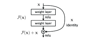
Figure 1: Residual Network skip connection block.

2.2 Multicriteria optimization

Multiple Criteria Decision-Making (MCDM) is a branch of Operations Research and Management Science. MCDM represents the set of methods and processes through which the concern for several conflicting criteria can be explicitly incorporated into the analytical process Ehrgott et al., (2002). Several strategies, spanning from a priori to interactive ones, have been developed to address this issue (Miettinen,, 2012). Historically MCDM’s first roots are the ones laid by Pareto at the end of the 19th century. However, the modern MCDM has its origins more recently in the work of Koopmans, (1951) who modified the canonical single objective linear programming model by reframing it as a vector optimization problem. An MCDM problem takes the following form:

$$\min_{\boldsymbol{x}} \{f_{1}(\boldsymbol{x}),f_{2}(\boldsymbol{x}),\dots,f_{k}(\boldsymbol{x})\}$$ (3)

subject to $$\boldsymbol{x}\in S$$ (4)

where $f_{i}:{\rm I\!R}^{n}\rightarrow{\rm I\!R}$ is the ith objective and the vector $\boldsymbol{x}$ contains the decision variables that belong to the feasible set $S$. Scalarization is a common approach for dealing with Multicriteria optimization problems. By scalarization, a vector optimization problem turns into a single objective optimization problem. Additional concerns affect the DM’s preferences scheme as a result of this. In our approach, we begin by using a weighted sum scalarization to handle our problem:

$$\min_{\boldsymbol{x}} \boldsymbol{w}^{\top}\boldsymbol{f}(\boldsymbol{x})$$ (5)

subject to $$\boldsymbol{x}\in S$$ (6)

where the weights are the relative preference of the DM toward a specific goal. The incorporation of such preferences can happen in two ways, either a priori or a posteriori. In our approach, we use an a posteriori method as this best suits the DM’s lack of knowledge, which may be uncertain about the relative importance of each objective.

2.3 Knowledge injection

Knowledge in this paper is intended as validated information about relations between entities in specific contexts as in von Rueden et al., (2021). The key feature of such a definition is that it allows for formalization, implying that such knowledge can be transformed into mathematical constraints somehow.

Let’s assume we have a deep architecture such that $\hat{y}=\mathcal{F}(\boldsymbol{x},\mathcal{W})$ and we observe the true label $y$ then we can train a supervised model by using a differentiable loss function as for the case of regression by using the mean squared error (MSE):

$$Loss_{f}(\boldsymbol{x},\mathcal{W})=\frac{1}{n}\sum_{i=1}^{n}(y_{i}-\hat{y}_{i})^{2}$$ (7)

or in our case, of a binary classification with the binary cross-entropy:

$$Loss_{f}(\boldsymbol{x},\mathcal{W})=\frac{1}{n}\sum_{i=1}^{n}\left[y_{i}\log(\hat{y}_{i}+(1-y_{i})\log(1-\hat{y}_{i})\right]$$ (8)

this will constitute the first objective of our Multicriteria loss function, that is, data fitting. The knowledge injection instead will act on the features’ effects on the model outcome, which means that our knowledge-based objective will be:

$$Loss_{k}(\boldsymbol{x},\mathcal{W})=k(\boldsymbol{x})\odot\frac{\delta\mathcal{F}(\boldsymbol{x},\mathcal{W})}{\delta\boldsymbol{x}}$$ (9)

where the right-hand side of the Hadamard product is the gradient of our DL model at the feature level $\boldsymbol{x}$ whereas $k(\boldsymbol{x})$ is a function that penalizes/favorites specific effect of the gradient with range $[-1,1]$. Since knowledge is hardly spread through the whole feature space, a possible strategy is to define $k(\boldsymbol{x})$ that maps the feature space to the knowledge we expect on that particular feature neighbor.

In its most straightforward formulation, $k(\boldsymbol{x})$ can be a scalar, and in this formulation is easier to investigate its behavior at the model level. Let us assume $k(\boldsymbol{x})=\boldsymbol{1}$ then what is enforced is that all partial derivatives should be negative therefore enforcing monotonicity and, in particular decreasing monotonicity. The opposite holds for the case when $k(\boldsymbol{x})=\boldsymbol{-1}$. When $k(\boldsymbol{x})=\boldsymbol{0}$ there is no constraint on the gradient behavior, meaning that knowledge is non-existent and therefore not injected. Following Daw et al., (2021) we can augment our Multicriteria function with a further constraint that measures the network complexity as, for example, an $L_{2}$ regularization on the weights. The result is the following unconstrained minimization problem:

$$\min_{\mathcal{W}}\boldsymbol{\lambda}^{\top}\begin{bmatrix}Loss_{f}(\boldsymbol{x},\mathcal{W})\\ ||\mathcal{W}||_{2}\\ Loss_{k}(\boldsymbol{x},\mathcal{W})\end{bmatrix}$$ (10)

2.4 Interpretability methods

Model interpretability is gaining popularity due to the increasing applications of non-linear models (Molnar et al.,, 2020). Model-agnostic and model-aware approaches are the two main types of interpretability approaches. The model is never accessed in model-agnostic interpretability methods. Unlike the model-agnostic approach, the model-aware technique has access to model parameters such as the gradient. Model-agnostic methods apply to all models, whereas model-aware are restricted to a specific class of models. On the other hand, model-aware approaches are more efficient and converge faster to the genuine interpretability metric.

2.4.1 Model-aware interpretability

One of the first techniques proposed by the literature was to use the product of the model’s gradient with feature values (Baehrens et al.,, 2010). Simonyan et al., (2014) proposed Saliency Maps based on the gradient of model output with respect to the input features. In other words, the score of multiclass $c$ classifier can be locally approximated by:

$$S_{c}(I)\approx w_{c}^{T}I+b_{c}$$ (11)

where $w_{c}^{T}$ is the gradient of the model at that particular class $c$ in that particular feature configuration $I_{0}$:

$$w=\frac{\partial S_{c}}{\partial I}\Bigr{|}_{I_{0}}$$ (12)

Sundararajan et al., (2017) through an axiomatic approach, questioned the validity of such procedure, arguing that using only the gradient may result in misleading feature attributions with respect to a baseline observation. They proposed the concept of Integrated Gradients, a path-dependent approach in which the gradients are accumulated over the linear combinations between the observation and a baseline. This implies the evaluation of the following:

$$IG_{0}=(I_{0}-I^{\prime})\int^{1}_{\alpha=0}\frac{\partial S_{c}(I^{\prime}+\alpha(I_{0}-I^{\prime})}{\partial I}d\alpha$$ (13)

2.4.2 Model-agnostic interpretability

One of the first model-agnostic technique was the Partial Dependence (PD) proposed by Friedman, (1991). PD plots evaluate the change in the average predicted value, as specified features vary over their marginal distribution Goldstein et al., (2015). However the main limitation of the PD is the dependence within features since evaluating the PD carries the risk of computing points outside the data envelope. Apley and Zhu, (2020) proposed the Accumulated Local Effects (ALEs) to address this flaw. ALEs have the advantage of avoiding the problem of evaluating variables’ effects outside the data envelope (Apley and Zhu,, 2020). Computing the ALE implies the evaluation of the following:

$$ALE_{\hat{f},S}(x_{S})=\sum_{k=1}^{k_{S}(x)}\frac{1}{n_{S}(k)}\sum_{i:x_{S}^{(i)}\in N_{S}(k)}\left[\hat{f}(z_{k,j},x_{\setminus S}^{(i)})-\hat{f}(z_{k-1,j},x_{\setminus S}^{(i)})\right]-C$$ (14)

where: $\hat{f}$ is the black-box model, $S$ is the subset of variables’ index, $X$ is the matrix containing all the variables, $x$ is the vector containing the feature values per observation, $z$ identifies the boundaries of the K partitions, such that $z_{0,S}=min(x_{S})$, $C$ is a constant term to center the plot. To make Equation 14 model-aware we can substitute finite differences with the gradient as $\frac{\delta\hat{f}(z_{S},X_{\setminus S})}{\delta z_{S}}\approx\hat{f}(z_{k,j},x_{\setminus S}^{(i)})-\hat{f}(z_{k-1,j},x_{\setminus S}^{(i)})$. Because of that, the resulting model-aware formula is:

$$ALE_{\hat{f},S}(x)=\int_{z_{0,S}}^{x}\left[\int\frac{\delta\hat{f}(z_{S},X_{\setminus S})}{\delta z_{S}}d\mathcal{P}(X_{\setminus S}|z_{S})\right]dz_{S}-C$$ (15)

As a result, knowledge injection, as proposed in the previous section, will have an effect on the ALEs because the final model will have a different gradient than the non-knowledge injected one.

3 Data, software, hardware

3.1 Data

To test the goodness of our approach, we provide an empirical application in the context of credit risk. In particular on the problem of bankruptcy prediction. We used a publicly available dataset of Polish enterprises donated to the UCI Machine Learning Repository by Zikeba et al., (2016). The data contains information about the financial conditions of Polish companies belonging to the manufacturing sector. The dataset contains 64 financial ratios ranging from liquidity to leverage measures . Moreover, the dataset distinguishes five classification cases that depend on the forecasting period. In our empirical setting, we focus on bankruptcy status after one year. In this subset of data, the total number of observations is 5910, out of which only 410 represents bankrupted firms. It is worth noting that we do not counter the class imbalance in the empirical setting, although this is something done commonly in the literature. We retained class imbalance to test the robustness of our approach even in conditions of scarcity of a particular class and used robust metrics such as the Area Under the Receiving Operating Curve (AUROC). Moreover, as our empirical experiment focuses on testing our approach on model interpretability, we restricted the number of features we considered to six. This is due to the fact that ALEs are inspected as plots, and having a plot for each feature increases complexity without providing any additional benefit to the reader or our approach. The choice was to focus on Attr 13, Attr 16, Attr 23, Attr 24, Attr 26, and Attr 27. The attributes were selected by using a ROC-based feature selection (Kuhn and Johnson,, 2019).

3.2 Software and hardware

The overall pipeline management is built in R (R Core Team,, 2020). The preprocessing relied on the tidymodels ecosystem (Kuhn and Wickham,, 2020) as well as on the tidyverse (Wickham et al.,, 2019). The DL models are developed in Julia (Bezanson et al.,, 2017) using the Flux framework (Innes et al.,, 2018; Innes,, 2018). The interoperability between the two languages is possible via the JuliaConnectoR library (Lenz et al.,, 2021). To debug the model and to check the validity of our approach, we employed the ALEPlot package (Apley,, 2018). As for the hardware environment, the pipeline is carried out on a local machine with 12 logical cores (Intel i7-9850H), 16 GB RAM, and a Cuda enabled graphic card (NVIDIA Quadro T2000). Both Julia and R codes are freely available for research reproducibility on GitLab, and an ad-hoc Docker container has been created on DockerHub.

4 Results

To test the performance of our approach on the Polish firms’ dataset, we use a standard practice in the field of DL. At first, we split the dataset into training and testing. Three-quarters of the dataset is for training the model and the rest for testing its performance. In the case of a model that contains no hyperparameters, a setting like this will suffice. However, in DL, this is never the case as these models require a thorough calibration of hyperparameters. In our setup, the hyperparameters are the elements contained in $\boldsymbol{\lambda}$. Therefore a common strategy is to use the training set to do what is called hyperparameter optimization (Goodfellow et al.,, 2016). Therefore, the training set is further divided into training and validation sets, and the model is fitted and validated with different parameters. In our case, we draw from the training set ten samples using the bootstrap technique as proposed by Efron and Tibshirani, (1997), and we trained our model using different combinations of hyperparameters. As for the choice on implementing such hyperparameter search, we relied on grid search, also known as full factorial design (Montgomery,, 2017). We then trained the model on the entire training set and classified bankruptcy state on the test set with the optimal hyperparameters.

For a deep understanding of the results, we divided the analysis into three parts. Firstly we performed hyperparameter optimization and subsequent hold-out testing using both the MLP and the RN, with the former being the best performing model. Secondly, with the MLP, we analyzed the effect on the interpretation by using ALE plots. Thirdly we tested the robustness of our approach by diminishing the amount of data.

4.1 Performance review

Table 1 presents the mean AUROC as well as its standard errors as our model validation involved ten bootstrap samples. The first striking result is that both the MLP and RN perform poorly without any regularization nor knowledge injection. This result is in line with Zikeba et al., (2016), which also found that the ANN architectures suffer in terms of generalization. What instead is of great interest is the increase in performance when both regularisation and knowledge injection are brought to the table. In particular, the ResNet seems to perform better with low levels of knowledge injection and a modest level of regularization. However, what is more, relevant is the behavior of the MLP. The model is more sensitive to knowledge injection and performs significantly better in model validation. This result is evident when $\lambda_{3}=0.3$, all the MLP models are above an AUROC of $0.8$ with a modest amount of standard error. Another significant result of the MLP is performance deterioration when regularization starts to ramp $\lambda_{2}=0.3$ up even with injected knowledge. What is worth noting is that the dataset suffers from significant class imbalance, and nothing has been done to alleviate it to test the effectiveness of our approach in such context. Indeed knowledge injection alleviates misclassification and creates a model that is on par with other robust classifiers.

Table 1: Performances of Multilayer Perceptron and Residual Network on the training set with various hyperparameter settings. The performance is measured as the mean and standard errors of the Area Under the Receiving Operating Curve in each bootstrap sample. Bold values indicate the best performing hyperparametrization for each model.

				Multilayer Perceptron			Residual Network
$\lambda_{1}$	$\lambda_{2}$	$\lambda_{3}$		Mean	Standard error		Mean	Standard error
1.0	0.0	0.0		0.6585	0.0178		0.5061	0.0843
0.9	0.1	0.0		0.6924	0.0111		0.5308	0.0805
0.8	0.2	0.0		0.6302	0.0757		0.6326	0.0180
0.7	0.3	0.0		0.7175	0.0059		0.5584	0.0900
0.9	0.0	0.1		0.7905	0.0087		0.6418	0.0740
0.8	0.1	0.1		0.8286	0.0149		0.5744	0.0769
0.7	0.2	0.1		0.7586	0.0336		0.5059	0.0746
0.6	0.3	0.1		0.6163	0.1219		0.6604	0.0879
0.8	0.0	0.2		0.8263	0.0129		0.5124	0.0664
0.7	0.1	0.2		0.8242	0.0170		0.6102	0.0186
0.6	0.2	0.2		0.8206	0.0123		0.5037	0.0443
0.5	0.3	0.2		0.7617	0.0601		0.6249	0.0593
0.7	0.0	0.3		0.8202	0.0119		0.6074	0.0172
0.6	0.1	0.3		0.8289	0.0139		0.5410	0.0417
0.5	0.2	0.3		0.8306	0.0135		0.5318	0.0150
0.4	0.3	0.3		0.8178	0.0198		0.5628	0.0378

The performances in Table 1 are promising. However, to precisely measure model generalization error, the performances that need to be considered are those taken from the test set. Table 2 presents these performances by taking into account only the optimally parametrized models and their baseline, that is, the model with $\lambda_{1}=1$. The clear-cut result from this table is that the MLP generalizes way better than its counterpart, with a slight decrease in performance in line with the expectations. This result suggests that knowledge injection corroborated with mild regularization can enhance the generalization performances of a DL classifier as the MLP and make it robust to class imbalances.

Table 2: Performances of Multilayer Perceptron and Residual Network on the test set with validated and baseline hyperparameter settings. The performance is measured as the Area Under the Receiving Operating Curve in the test sample.

$\lambda_{1}$	$\lambda_{2}$	$\lambda_{3}$	Multilayer Perceptron	Residual Network
1.0	0.0	0.0	0.577	0.582
0.5	0.2	0.3	0.821	-
0.4	0.3	0.1	-	0.518

In the following sections, we will investigate further the performance of the MLP with and without knowledge injection in terms of interpretability and robustness to data scarcity. We will focus only on the MLP, as it was the most performant architecture. Moreover, analyzing the interpretations of a non-performant classifier as the RN has no useful meaning from a practical point of view.

4.2 Interpretability review

A mentioned in the previous sections, post-hoc interpretability methods are essential tools for model debugging and to inspect any model bias. As a result, we present figure 2(a), which demonstrates MLP ALEs with and without knowledge injection. The ALEs of the model without knowledge injection show several misbehaviors that may be due to class imbalance or hidden biases in the training sample. In detail:

• Attr 13: which is also known as the EBITDA-To-Sales ratio, is a profitability indicator. Therefore we should expect to decrease the probability of bankruptcy, especially in cases where the ratio is positive. The opposite occurs instead. An increase of the ratio above zero increases the probability of bankruptcy. This effect is at odds with the literature on the subject as, for example, in Platt and Platt, (2002).

• Attr 16: is the inverse and a proxy of the Debt-To-EBITDA ratio which is leverage ratio. For the inverse of a leverage ratio we would assume negative impact on bankruptcy as in Beaver, (1968).

• Attr 23: is the Net profit ratio and is a productivity ratio Lee and Choi, (2013) which tends to have a negative impact on bankruptcy.

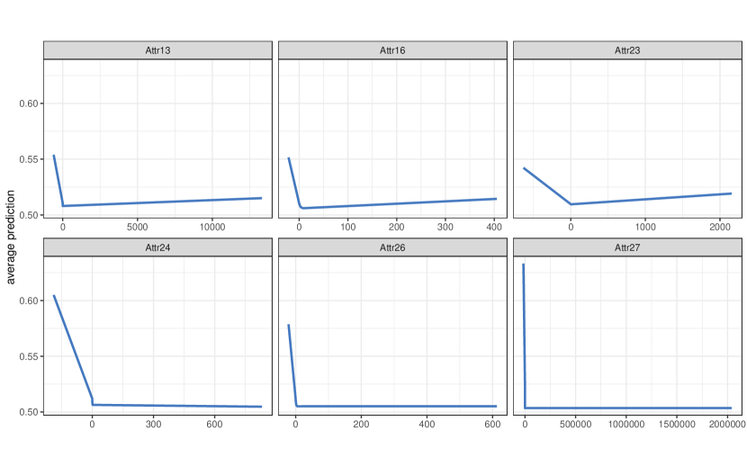
(a) Accumulated Local Effects plot of the Multilayer Perceptron architecture, without regularization and knowledge injection (i.e. $\lambda_{1}=1,\lambda_{2}=0.0,\lambda_{3}=0.0$).

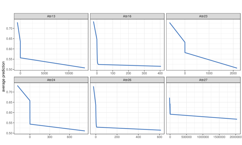
(b) Accumulated Local Effects plot of the Multilayer Perceptron architecture, with regularisation and knowledge injection optimally selected from the hyperparameter optimization procedure (i.e. $\lambda_{1}=0.5,\lambda_{2}=0.2,\lambda_{3}=0.3$).

Figure 2: Accumulated Local Effects plot of the Multilayer Perceptron architecture, with and without regularization and knowledge injection.

To counter this common biased effects we assumed the following logistic form for all the features’ knowledge function:

$$k(x)=\frac{1}{1+e^{-100x}}$$ (16)

Such a knowledge function penalizes only positive effects above zero and retains the correctly captured effects below it. With this setting, in the case of moderate knowledge injection, the effects align with the literature findings.

4.3 Robustness checks

A fundamental question is how model performances deteriorate with less training data. In previous works, knowledge injection has been implemented indeed to alleviate such problems as in von Kurnatowski et al., (2021). To discover how our approach deals with scarce data, we systematically diminished the training set and measured the corresponding performance on the test set. These results are in Table 3 which depicts the different performances in the test set as the training data proportion decreases. In concordance with the literature on knowledge injection, our approach prevents performance degradation even in extreme cases where only half the dataset is used for training.

Table 3: Performances of Multilayer Perceptron on the test set under different proportions of train/test split. The performance is measured as the Area Under the Receiving Operating Curve in the test sample.

Train/Test	With knowledge ($\lambda_{1}=0.5,\lambda_{2}=0.2,\lambda_{3}=0.3$)	Without knowledge ($\lambda_{1}=0.1,\lambda_{2}=0.0,\lambda_{3}=0.0$)
0.85	0.829	0.615
0.80	0.828	0.543
0.75	0.821	0.577
0.7	0.822	0.605
0.65	0.790	0.613
0.6	0.817	0.646
0.55	0.803	0.505
0.5	0.823	0.641

5 Conclusion

In this paper, we presented a novel approach to knowledge injection at the level of feature effects of a DL model. Model interpretability is a particularly crucial topic, and recent legislation implies interpretability from the start. Recent post-hoc interpretability methods fail to provide this. Our approach solves the problem by allowing to control model interpretation from the start. The approach consists in solving a Multicriteria minimization problem in which knowledge adherence competes with greedy data fitting and regularization. We accounted for partial knowledge and nonlinearity by defining ad-hoc knowledge functions on the model’s parameters. We presented a use case of bankruptcy prediction using a Polish firm’s dataset to test our approach. The results suggest that knowledge injection improves performances and keeps model interpretation in line with the literature findings, avoiding idiosyncratic effects resulting from either class imbalance or possible biases in the dataset. The DM can check the effects of our approach through post-hoc interpretability methods that play a crucial role in fine-tuning the model before production. Another critical question that we answered is model performance degradation in case of data shortage. Our results suggest that knowledge injection gives the modeler more freedom in terms of the necessary data for proper model training.

This new methodology creates many new opportunities in terms of research. One possible further research can be the investigation of more complex knowledge functions. A second research path would be to enforce knowledge consistency within different scenarios, as in the case of time series. These are only a few possible new research efforts that will pave the way for knowledge-informed DL.

Appendix A Dataset indicators

Table 4: Dataset financial indicators with corresponding description.

ID	Description	ID	Description
Attr 1	net profit / total assets	Attr 33	operating expenses / short-term liabilities
Attr 2	total liabilities / total assets	Attr 34	operating expenses / total liabilities
Attr 3	working capital / total assets	Attr 35	profit on sales / total assets
Attr 4	current assets / short-term liabilities	Attr 36	total sales / total assets
Attr 5	[(cash + short-term securities + receivables - short-term liabilities) / (operating expenses - depreciation)] * 365	Attr 37	(current assets - inventories) / long-term liabilities
Attr 6	retained earnings / total assets	Attr 38	constant capital / total assets
Attr 7	EBIT / total assets	Attr 39	profit on sales / sales
Attr 8	book value of equity / total liabilities	Attr 40	(current assets - inventory - receivables) / short-term liabilities
Attr 9	sales / total assets	Attr 41	total liabilities / ((profit on operating activities + depreciation) * (12/365))
Attr 10	equity / total assets	Attr 42	profit on operating activities / sales
Attr 11	(gross profit + extraordinary items + financial expenses) / total assets	Attr 43	rotation receivables + inventory turnover in days
Attr 12	gross profit / short-term liabilities	Attr 44	(receivables * 365) / sales
Attr 13	(gross profit + depreciation) / sales	Attr 45	net profit / inventory
Attr 14	(gross profit + interest) / total assets	Attr 46	(current assets - inventory) / short-term liabilities
Attr 15	(total liabilities * 365) / (gross profit + depreciation)	Attr 47	(inventory * 365) / cost of products sold
Attr 16	(gross profit + depreciation) / total liabilities	Attr 48	EBITDA (profit on operating activities - depreciation) / total assets
Attr 17	total assets / total liabilities	Attr 49	EBITDA (profit on operating activities - depreciation) / sales
Attr 18	gross profit / total assets	Attr 50	current assets / total liabilities
Attr 19	gross profit / sales	Attr 51	short-term liabilities / total assets
Attr 20	(inventory * 365) / sales	Attr 52	(short-term liabilities * 365) / cost of products sold)
Attr 21	sales (n) / sales (n-1)	Attr 53	equity / fixed assets
Attr 22	profit on operating activities / total assets	Attr 54	constant capital / fixed assets
Attr 23	net profit / sales	Attr 55	working capital
Attr 24	gross profit (in 3 years) / total assets	Attr 56	(sales - cost of products sold) / sales
Attr 25	(equity - share capital) / total assets	Attr 57	(current assets - inventory - short-term liabilities) / (sales - gross profit - depreciation)
Attr 26	(net profit + depreciation) / total liabilities	Attr 58	total costs /total sales
Attr 27	profit on operating activities / financial expenses	Attr 59	long-term liabilities / equity
Attr 28	working capital / fixed assets	Attr 60	sales / inventory
Attr 29	logarithm of total assets	Attr 61	sales / receivables
Attr 30	(total liabilities - cash) / sales	Attr 62	(short-term liabilities *365) / sales
Attr 31	(gross profit + interest) / sales	Attr 63	sales / short-term liabilities
Attr 32	(current liabilities * 365) / cost of products sold	Attr 64	sales / fixed assets

References

- Abadi et al., (2015) Abadi, M., Agarwal, A., Barham, P., Brevdo, E., Chen, Z., Citro, C., Corrado, G. S., Davis, A., Dean, J., Devin, M., Ghemawat, S., Goodfellow, I., Harp, A., Irving, G., Isard, M., Jia, Y., Jozefowicz, R., Kaiser, L., Kudlur, M., Levenberg, J., Mané, D., Monga, R., Moore, S., Murray, D., Olah, C., Schuster, M., Shlens, J., Steiner, B., Sutskever, I., Talwar, K., Tucker, P., Vanhoucke, V., Vasudevan, V., Viégas, F., Vinyals, O., Warden, P., Wattenberg, M., Wicke, M., Yu, Y., and Zheng, X. (2015). TensorFlow: Large-scale machine learning on heterogeneous systems.
- Altman, (1968) Altman, E. I. (1968). Financial ratios, discriminant analysis and the prediction of corporate bankruptcy. The journal of finance, 23(4):589–609.
- Altman and Sabato, (2007) Altman, E. I. and Sabato, G. (2007). Modelling Credit Risk for SMEs: Evidence from the U.S. Market. Abacus, 43(3):332–357.
- Apley, (2018) Apley, D. (2018). ALEPlot: Accumulated Local Effects (ALE) Plots and Partial Dependence (PD) Plots.
- Apley and Zhu, (2020) Apley, D. W. and Zhu, J. (2020). Visualizing the effects of predictor variables in black box supervised learning models. Journal of the Royal Statistical Society: Series B (Statistical Methodology), 82(4):1059–1086.
- Arifovic and Gencay, (2001) Arifovic, J. and Gencay, R. (2001). Using genetic algorithms to select architecture of a feedforward artiÿcial neural network. Physica A, page 21.
- Baehrens et al., (2010) Baehrens, D., Schroeter, T., Harmeling, S., Kawanabe, M., Hansen, K., and Müller, K.-R. (2010). How to explain individual classification decisions. The Journal of Machine Learning Research, 11:1803–1831.
- Beaver, (1968) Beaver, W. H. (1968). Alternative accounting measures as predictors of failure. The accounting review, 43(1):113–122.
- Bezanson et al., (2017) Bezanson, J., Edelman, A., Karpinski, S., and Shah, V. B. (2017). Julia: A fresh approach to numerical computing. SIAM review, 59(1):65–98.
- Bottou et al., (2007) Bottou, L., Chapelle, O., DeCoste, D., and Weston, J. (2007). Scaling Learning Algorithms toward AI. In Large-Scale Kernel Machines, pages 321–359. MIT Press.
- Bücker et al., (2021) Bücker, M., Szepannek, G., Gosiewska, A., and Biecek, P. (2021). Transparency, auditability, and explainability of machine learning models in credit scoring. Journal of the Operational Research Society, pages 1–21.
- Ciampi et al., (2021) Ciampi, F., Giannozzi, A., Marzi, G., and Altman, E. I. (2021). Rethinking SME default prediction: A systematic literature review and future perspectives. Scientometrics, pages 1–48.
- Ciampi and Gordini, (2013) Ciampi, F. and Gordini, N. (2013). Small enterprise default prediction modeling through artificial neural networks: An empirical analysis of Italian small enterprises. Journal of Small Business Management, 51(1):23–45.
- Daw et al., (2021) Daw, A., Karpatne, A., Watkins, W., Read, J., and Kumar, V. (2021). Physics-guided Neural Networks (PGNN): An Application in Lake Temperature Modeling. arXiv:1710.11431 [physics, stat].
- Dexe et al., (2020) Dexe, J., Ledendal, J., and Franke, U. (2020). An Empirical Investigation of the Right to Explanation Under GDPR in Insurance. In Gritzalis, S., Weippl, E. R., Kotsis, G., Tjoa, A. M., and Khalil, I., editors, Trust, Privacy and Security in Digital Business, Lecture Notes in Computer Science, pages 125–139, Cham. Springer International Publishing.
- Efron and Tibshirani, (1997) Efron, B. and Tibshirani, R. (1997). Improvements on Cross-Validation: The 632+ Bootstrap Method. Journal of the American Statistical Association, 92(438):548–560.
- Ehrgott et al., (2002) Ehrgott, M., Gandibleux, X., and Hillier, F. S., editors (2002). Multiple Criteria Optimization: State of the Art Annotated Bibliographic Surveys, volume 52 of International Series in Operations Research & Management Science. Springer US, Boston, MA.
- European Commission, (2019) European Commission (2019). Ethics guidelines for trustworthy AI. Technical report.
- Friedman, (1991) Friedman, J. H. (1991). Multivariate Adaptive Regression Splines. The Annals of Statistics, 19(1):1–67.
- Goldstein et al., (2015) Goldstein, A., Kapelner, A., Bleich, J., and Pitkin, E. (2015). Peeking Inside the Black Box: Visualizing Statistical Learning With Plots of Individual Conditional Expectation. Journal of Computational and Graphical Statistics, 24(1):44–65.
- Goodfellow et al., (2016) Goodfellow, I., Bengio, Y., and Courville, A. (2016). Deep Learning. MIT Press.
- He et al., (2015) He, K., Zhang, X., Ren, S., and Sun, J. (2015). Deep Residual Learning for Image Recognition. arXiv:1512.03385 [cs].
- Innes, (2018) Innes, M. (2018). Flux: Elegant machine learning with julia. Journal of Open Source Software.
- Innes et al., (2018) Innes, M., Saba, E., Fischer, K., Gandhi, D., Rudilosso, M. C., Joy, N. M., Karmali, T., Pal, A., and Shah, V. (2018). Fashionable modelling with flux. CoRR, abs/1811.01457.
- Koopmans, (1951) Koopmans, T. (1951). Analysisofproductionasanefficientcombinationofactivities. Activityanalysisofproductionandallocation, TC Koopmans, editor, Wiley, New York.
- Kotłowski and Słowiński, (2009) Kotłowski, W. and Słowiński, R. (2009). Rule learning with monotonicity constraints. In Proceedings of the 26th Annual International Conference on Machine Learning, ICML ’09, pages 537–544, New York, NY, USA. Association for Computing Machinery.
- Kuhn and Johnson, (2019) Kuhn, M. and Johnson, K. (2019). Feature Engineering and Selection: A Practical Approach for Predictive Models. CRC Press.
- Kuhn and Wickham, (2020) Kuhn, M. and Wickham, H. (2020). Tidymodels: A Collection of Packages for Modeling and Machine Learning Using Tidyverse Principles.
- Lauer and Bloch, (2008) Lauer, F. and Bloch, G. (2008). Incorporating Prior Knowledge in Support Vector Machines for Classification: A Review. Neurocomputing, 71(7-9):1578–1594.
- LeCun et al., (1990) LeCun, Y., Boser, B., Denker, J., Henderson, D., Howard, R., Hubbard, W., and Jackel, L. (1990). Handwritten Digit Recognition with a Back-Propagation Network. In Advances in Neural Information Processing Systems, volume 2. Morgan-Kaufmann.
- Lee and Choi, (2013) Lee, S. and Choi, W. S. (2013). A multi-industry bankruptcy prediction model using back-propagation neural network and multivariate discriminant analysis. Expert Systems with Applications, 40(8):2941–2946.
- Lenz et al., (2021) Lenz, S., Hackenberg, M., and Binder, H. (2021). The JuliaConnectoR: A functionally oriented interface for integrating Julia in R. arXiv:2005.06334 [cs, stat].
- Lessmann et al., (2015) Lessmann, S., Baesens, B., Seow, H.-V., and Thomas, L. C. (2015). Benchmarking state-of-the-art classification algorithms for credit scoring: An update of research. European Journal of Operational Research, 247(1):124–136.
- McCulloch and Pitts, (1943) McCulloch, W. S. and Pitts, W. (1943). A logical calculus of the ideas immanent in nervous activity. The bulletin of mathematical biophysics, 5(4):115–133.
- Miettinen, (2012) Miettinen, K. (2012). Nonlinear Multiobjective Optimization, volume 12. Springer Science & Business Media.
- Molnar et al., (2020) Molnar, C., Casalicchio, G., and Bischl, B. (2020). Interpretable Machine Learning – A Brief History, State-of-the-Art and Challenges. In Koprinska, I., Kamp, M., Appice, A., Loglisci, C., Antonie, L., Zimmermann, A., Guidotti, R., Özgöbek, Ö., Ribeiro, R. P., Gavaldà, R., Gama, J., Adilova, L., Krishnamurthy, Y., Ferreira, P. M., Malerba, D., Medeiros, I., Ceci, M., Manco, G., Masciari, E., Ras, Z. W., Christen, P., Ntoutsi, E., Schubert, E., Zimek, A., Monreale, A., Biecek, P., Rinzivillo, S., Kille, B., Lommatzsch, A., and Gulla, J. A., editors, ECML PKDD 2020 Workshops, Communications in Computer and Information Science, pages 417–431, Cham. Springer International Publishing.
- Montgomery, (2017) Montgomery, D. C. (2017). Design and Analysis of Experiments. John wiley & sons.
- Muralidhar et al., (2018) Muralidhar, N., Islam, M. R., Marwah, M., Karpatne, A., and Ramakrishnan, N. (2018). Incorporating Prior Domain Knowledge into Deep Neural Networks. In 2018 IEEE International Conference on Big Data (Big Data), pages 36–45.
- Nosratabadi et al., (2020) Nosratabadi, S., Mosavi, A., Duan, P., Ghamisi, P., Filip, F., Band, S. S., Reuter, U., Gama, J., and Gandomi, A. H. (2020). Data Science in Economics: Comprehensive Review of Advanced Machine Learning and Deep Learning Methods. Mathematics, 8(10):1799.
- Ozbayoglu et al., (2020) Ozbayoglu, A. M., Gudelek, M. U., and Sezer, O. B. (2020). Deep learning for financial applications : A survey. Applied Soft Computing, 93:106384.
- Paszke et al., (2019) Paszke, A., Gross, S., Massa, F., Lerer, A., Bradbury, J., Chanan, G., Killeen, T., Lin, Z., Gimelshein, N., Antiga, L., Desmaison, A., Kopf, A., Yang, E., DeVito, Z., Raison, M., Tejani, A., Chilamkurthy, S., Steiner, B., Fang, L., Bai, J., and Chintala, S. (2019). PyTorch: An imperative style, high-performance deep learning library. In Wallach, H., Larochelle, H., Beygelzimer, A., dAlché-Buc, F., Fox, E., and Garnett, R., editors, Advances in Neural Information Processing Systems 32, pages 8024–8035. Curran Associates, Inc.
- Platt and Platt, (2002) Platt, H. D. and Platt, M. B. (2002). Predicting corporate financial distress: Reflections on choice-based sample bias. Journal of economics and finance, 26(2):184–199.
- R Core Team, (2020) R Core Team (2020). R: A Language and Environment for Statistical Computing. R Foundation for Statistical Computing, Vienna, Austria.
- Rao and Frtunikj, (2018) Rao, Q. and Frtunikj, J. (2018). Deep learning for self-driving cars: Chances and challenges. In Proceedings of the 1st International Workshop on Software Engineering for AI in Autonomous Systems, SEFAIS ’18, pages 35–38, New York, NY, USA. Association for Computing Machinery.
- Rosenblatt, (1958) Rosenblatt, F. (1958). The perceptron: A probabilistic model for information storage and organization in the brain. Psychological Review, 65(6):386–408.
- Rudin, (2019) Rudin, C. (2019). Stop explaining black box machine learning models for high stakes decisions and use interpretable models instead. Nature Machine Intelligence, 1(5):206–215.
- Rumelhart et al., (1986) Rumelhart, D. E., McClelland, J. L., and Group, P. R. (1986). Parallel Distributed Processing: Explorations in the Microstructure of Cognition: Foundations, volume 1. A Bradford Book, Cambridge, MA, USA.
- Saad, (1998) Saad, D., editor (1998). On-Line Learning in Neural Networks. Publications of the Newton Institute. Cambridge University Press, Cambridge, [Eng.] ; New York.
- Simonyan et al., (2014) Simonyan, K., Vedaldi, A., and Zisserman, A. (2014). Deep Inside Convolutional Networks: Visualising Image Classification Models and Saliency Maps. arXiv:1312.6034 [cs].