Towards Robust and Automatic Hyper-Parameter Tunning

Abstract

The task of hyper-parameter optimization (HPO) is burdened with heavy computational costs due to the intractability of optimizing both a model’s weights and its hyper-parameters simultaneously. In this work, we introduce a new class of HPO method and explore how the low-rank factorization of the convolutional weights of intermediate layers of a convolutional neural network can be used to define an analytical response surface [Bergstra and Bengio (2012)] for optimizing hyper-parameters, using only training data. We quantify how this surface behaves as a surrogate to model performance and can be solved using a trust-region search algorithm, which we call autoHyper. The algorithm outperforms state-of-the-art such as Bayesian Optimization and generalizes across model, optimizer, and dataset selection. Our code can be found at https://github.com/MathieuTuli/autoHyper.

1 Introduction

Figure 1: Left: Validation Accuracy vs. Right: stable rank metric tracked autoHyper (see section 2)

The task of hyper-parameter optimization (HPO) is burdened with computational intractability caused by a dual-optimization problem, whereby optimization over a network’s weights as well as its hyper-parameters cannot happen simultaneously [Bergstra and Bengio (2012)]. The abstract formulation of HPO can be defined as
$\lambda^{*}\leftarrow\operatorname*{arg\,min}\limits_{\lambda\in\Lambda}\{\mathbb{E}_{x\sim M}[\mathcal{L}(x;\mathcal{A}_{\lambda}({X}^{(\text{train})})]\}$ as defined by Bergstra and Bengio (2012), where $X^{(\text{train})}$ and $x$ are random variables, modelled by some natural distribution $M$, that represent the train and validation data, respectively. $\mathcal{L}(\cdot)$ is some expected loss and $\mathcal{A}_{\lambda}({X}^{(\text{train})})$ is a learning algorithm that maps ${X}^{(\text{train})}$ to some learned function, conditioned on the hyper-parameter set $\lambda$. Note that this learned function, denoted as $f(\theta;\lambda;X^{(\text{train})})$, involves its own independent inner optimization problem. Because of this, optimization over the hyper-parameters $\lambda$ cannot occur until optimization over $f(\theta;\lambda;X^{(\text{train})})$ is complete. This means that HPO in this form suffers from heavy computational burden and is practically unsolvable. However, Bergstra and Bengio (2012) showed that this burden is reduced if we simplify our scope and only consider $\lambda^{*}\leftarrow\operatorname*{arg\,min}\limits_{\lambda\in\Lambda}\tau(\lambda)$ where, $\tau$ is called the response surface and $\Lambda$ is some set of choices for $\lambda$ (i.e. the search space). Simply put, the goal of the response surface is to act as an easier to solve surrogate function parameterized by $\lambda$ whose minimization is correlated to the minimization of our networks’s objective function. Importantly, this response surface is supposed to be much easier to solve for, and removes the dual-optimization problem.

Unfortunately, little advancements in an analytical model of the response surface $\tau$ has led to estimating it by (a) running multiple trials of different HP configurations (e.g. Random Search) against validation datassets; or (b) characterizing the distribution model of a certain configuration’s performance metric (e.g. validation performances) to numerically define a relationship between $\tau$ and $\lambda$ (e.g. Bayesian Optimization). Despite the success of these methods, they exist as estimations of a response surface, which is itself already a simplification/estimation of our initial objective function, which we argue is inefficient and sub optimal. We work towards resolving this issue.

In this paper, we deviate from existing classes of HPO methods and explore an alternative surrogate metric that demonstrates how to perform almost fully automatic HPO using only the training dataset. Our contributions are as follows: (1) stemming from the notion of stable rank in (Hosseini and Plataniotis, 2020; Jaegerman et al., 2021), we introduce the task of monitoring the well-posedness of learning layers in a Convolutional Neural Network (CNN) in order to develop a well-defined analytical response surface. Figure 1 shows how our new metric behaves well and tractably in contrast to conventional validation performance measures. This response surface deviates from existing works and exists as a new class of HPO; (2) we propose a trust-region search algorithm, dubbed autoHyper, to optimize our response surface and conduct HPO using only the training set. This algorithm almost eliminates all need for human intuition or manual intervention, and is not bound by a manually set searching space, paving the way towards automatic HPO; and (3), we extend the autoHyper algorithm to multi-dimensional HPO.

2 A New Response Surface Model

2.1 Stable Rank via Low-Rank Factorization

We wish to analyze the weight matrices of our neural network and develop a metric that we can track, per epoch, that acts as a surrogate to validation performance. To do so, we decompose the weight matrices of the network and study them by use of low-rank factorization, similar to what Hosseini et al. (2021) did for channel size optimization. Consider the 4-D tensor ${\bm{\mathsfit{W}}}\in\mathbb{R}^{N_{1}\times N_{2}\times N_{3}\times N_{4}}$ as the weights of a layer in a CNN ($N_{1}$ & $N_{2}$ being the height and width of kernel size, $N_{3}$ & $N_{4}$ the input and output channel size, respectively). We decompose ${\bm{\mathsfit{W}}}$ along some dimension $d$ as

$${\bm{\mathsfit{W}}}[\texttt{4-D Tensor}]\xrightarrow{\text{unfold}}{\bm{W}}_{d}[\texttt{2-D Matrix}]\xrightarrow{\text{factorize + decompose}}\widehat{{\bm{U}}}_{d}\widehat{\Sigma}_{d}\widehat{{\bm{V}}}_{d}^{T}+{\bm{E}}_{d}.$$

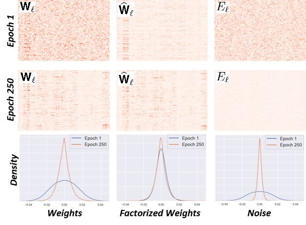
Figure 2: Low-Rank Decomposition (figure replicated from Hosseini et al. (2021))

We subsequently define $\widehat{{\bm{W}}}_{d}=\widehat{{\bm{U}}}_{d}\widehat{\Sigma}_{d}\widehat{{\bm{V}}}_{d}^{T}$ for simplicity, where $\widehat{{\bm{W}}}_{d}$ is the low-rank matrix containing limited non-zero singular values. We use the Variational Bayesian Matrix Factorization (VBMF) (Nakajima et al., 2013) for the low-rank factorization. This factorization is critical as it captures the presence of noise, allowing analysis to be invariant to the randomness of initialization. Note, unfolding isn’t necessary for linear layers (e.g. for LSTMs), and the analysis is the same. Through this factorization, initially, the low-rank component $\widehat{{\bm{W}}}_{d}$ has empty structure (i.e. $\widehat{{\bm{W}}}_{d}=\oslash$) as the randomness of the initialized weights is fully captured by ${\bm{E}}_{d}$. As training progresses, the low-rank component will gain structure and becomes non-empty as the network learns to map inputs to outputs. This is visualized in Figure 2 for a ResNet34 layer. Notice how the low-rank matrix maintains its structure and strengthens its structure over training, while the perturbing noise element decays. We state that such behaviour leads to a stabilized encoding layer and indicates a beneficial progress in learning. Following Hosseini and Plataniotis (2020), we define the stable rank of the weight matrix as

$${\mathcal{G}}_{d}(\widehat{{\bm{W}}}_{d})=\frac{1}{N_{d}\cdot\sigma_{1}(\widehat{{\bm{W}}}_{d})}\sum\limits_{i=1}^{N_{d}^{{}^{\prime}}}\sigma_{i}(\widehat{{\bm{W}}}_{d}),$$ (1)

where $\sigma_{1}\geq\sigma_{2}\geq\ldots\geq\sigma_{N_{d}}$ are low-rank singular values in descending order. Here $N_{d}=\rank\{\widehat{{\bm{W}}}_{d}\}$ and the unfolding is done either on input or output channels i.e. $d\in\{3,4\}$. We can further parameterize the stable rank ${\mathcal{G}}_{d}$ by the HP set $\lambda$, epoch $t$, and network layer $\ell$ as $\bar{{\mathcal{G}}}_{d,t,\ell}(\lambda)$. Note that $\bar{{\mathcal{G}}}_{d,t,\ell}(\lambda)\in[0,1]$ and is used to probe CNN layers to monitor how well information is carried from input to output maps. A perfect network and set of HPs would yield $\bar{{\mathcal{G}}}_{d,T,\ell}(\lambda)=1\quad\forall\ell\in[L]$, where $L$ is the network’ number of layers and $T$ is the last epoch. In this case, each layer is a near-perfect autoencoder and the information propagation through the network is maximized. Conversely, $\bar{{\mathcal{G}}}_{d,T,\ell}(\lambda)=0$ indicates that the information flow is very weak meaning the mapping is effectively random ($\parallel\!{\bm{E}}_{d}\!\parallel$ is maximized). See Appendix-A for further explanation.

2.2 Definition of New Response Function

If $\bar{{\mathcal{G}}}_{d,t,\ell}(\lambda)=0$ in early stages of training, no learning has occurred. This is due to the perturbing noise ${\bm{E}}_{d}$ being fully populated and the low-rank structure $\widehat{{\bm{W}}}_{d}$ being effectively empty. In practice, too small of an initial learning rate would also result in such a behaviour as insufficient progress has been made to reduce the randomization. We argue this becomes useful to track the number of layers with zero-valued ${\mathcal{G}}_{d}$ as we will subsequently aim to minimize this measure across the network. This effectively becomes a measure of channel rank, and we denote this rank per epoch as

$${\mathcal{Z}}_{t}(\lambda)\leftarrow\frac{1}{2L}\sum\limits_{\ell}^{L}\sum\limits_{d\in\{3,4\}}\mathbb{I}[\bar{{\mathcal{G}}}_{d,t,\ell}(\lambda)=0]~{}~{}~{}\text{where}~{}\mathbb{I}[\bar{{\mathcal{G}}}_{d,t,\ell}(\lambda)=0]=\left\{\begin{array}[]{ll}1&\textrm{if }\bar{{\mathcal{G}}}_{d,t,\ell}(\lambda)=0\\ 0&\textrm{otherwise}\end{array}\right.,$$

where $\mathcal{Z}_{t}(\lambda)\in[0,1)$. We pay no attention to which layers in particular have zero-valued ${\mathcal{G}}_{d}$; this could perhaps be explored in future work. The intuition behind averaging across all layers is to ensure that our model is “globally” optimized and not just locally within certain layers. Finally, we define the average rank across $T$ epochs – which we call the global stable rank – as

$${\mathcal{Z}}(\lambda)\leftarrow\frac{1}{T}\sum\limits_{t\in[T]}{\mathcal{Z}}_{t}(\lambda)~{}~{};~{}{\mathcal{Z}}(\lambda)\in[0,1).$$ (2)

This measure is therefore akin to a normalized summation of the zero-valued singular values from low-rank measures across all layers’ input and output unfolded-tensor arrays over $T$ epochs.

To solve for the optimal HP set $\lambda$, we state that this is achieved when the rate of change of ${\mathcal{Z}}(\lambda)$ first goes to zero. Visually, looking at Figure 3 (and Figures C.2 & C.3 in Appendix-C), the optimal HP is at the inception of the plateau in ${\mathcal{Z}}(\lambda)$. In support of this, we note that Wilson et al. (2017) found a more optimal learning rate for Adam applied to CIFAR10 to be $3\text{\times}{10}^{-4}$ instead of the author suggested $1\text{\times}{10}^{-3}$, and highlight how this value sits at the location we discuss here; the inception of the plateau in the rate of change of ${\mathcal{Z}}(\lambda)$. We formulate our response surface as

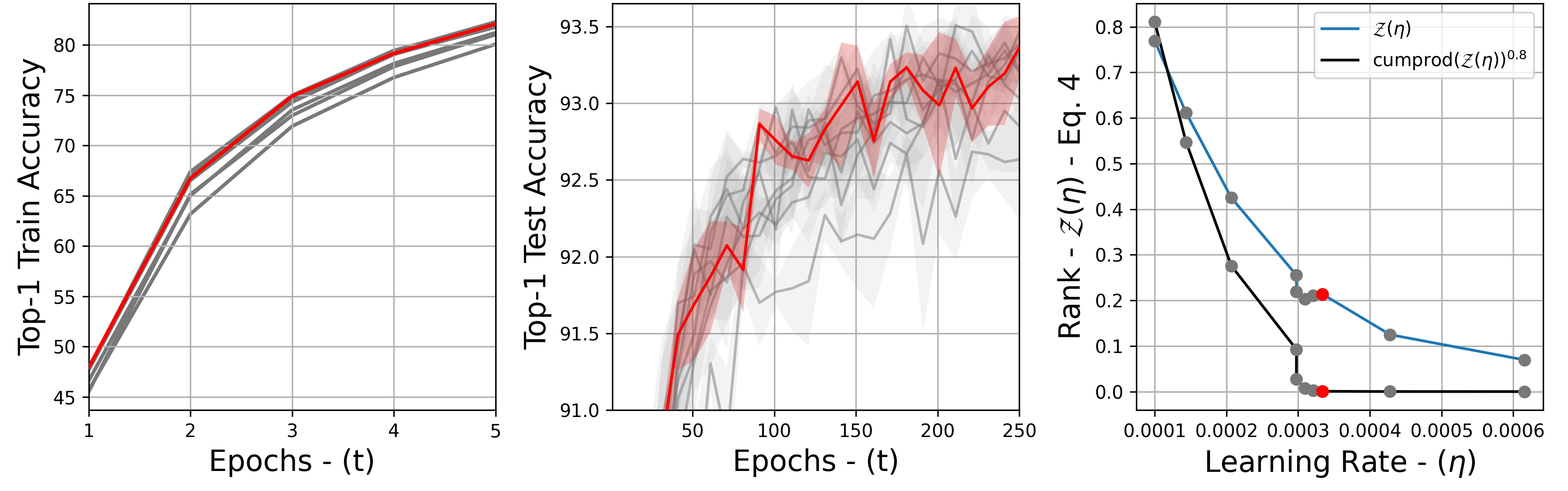
[Surrogate Behaviour] [2D Response Surface]

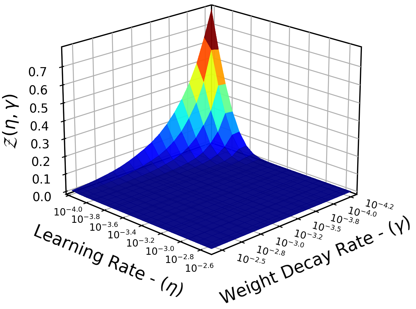
Figure 3: (a) Surrogate behaviour of ${\mathcal{Z}}(\eta)$ to training loss and accuracy. Red indicates the learning rate and model chosen by our method, with other trialled points in grayscale. (b) Two-dimensional response surface for $\lambda=\{\eta,\gamma\}$ for ResNet34 applied to CIFAR10, trained using Adam.

$$\lambda^{*}\leftarrow\operatorname*{arg\,min}_{\lambda}~{}[\tau(\lambda)=1-{\mathcal{Z}}(\lambda)~{}\text{subject to}~{}\parallel\nabla_{\lambda}{\mathcal{Z}}(\lambda)\parallel_{2}^{2}\leq\epsilon]$$

where $\epsilon\in[0,1)$ is a small error. We do not explicitly calculate the gradient $\nabla_{\lambda}{\mathcal{Z}}(\lambda)$, but use the rate of change to guide convergence towards the inception of the plateauing region (see section 3).

3 autoHyper: Automatic HP Tuning

Algorithm 1 autoHyper

0:  number of epochs $T=5$, starting $\lambda^{(0)}$

1:  $RH=[~{}]$ ; (empty list of rank histories)

2:  $j=0$

3:  while True do

4:     - compute trust-region $TR^{\lambda^{(j)}}$ for $\lambda^{(j)}$.

5:     for each permutation $\lambda^{(j*)}$ in $TR^{\lambda^{(j)}}$ do

6:        - train for $T$ epochs, record $\mathcal{Z}(\lambda^{(j*)})$

7:     if each of ${\mathcal{Z}}(\lambda^{(j*)})<0.9$ then

8:        - step in direction of max ${\mathcal{Z}}(\lambda^{(j*)})$

9:     else

10:        - $k\leftarrow\text{argmin}_{j*}~{}~{}\text{list of}~{}[{\mathcal{Z}}(\lambda^{(j*)})]$

11:        - $\lambda^{(j+1)}\leftarrow TR^{\lambda^{(j)}}[k]$

12:        - append smallest ${\mathcal{Z}}(\lambda^{(j*)})$ to $RH$

13:        - compute $cumprod(RH)^{0.8}$

14:     if rate of change plateaus then

15:        break

16:     $j\mathrel{+}=1$

How it works. The pseudo-code for autoHyper is presented in Algorithm 1. To find the inception of the plateuing region, autoHyper runs a trust-region optimization algorithm, where the trust-region is formed around the HP set, and stepping is made relative to our metric, ${\mathcal{Z}}(\lambda)$. That is, at each step, autoHyper computes the trust-region around its current HP set $\lambda$: For each HP in the set $\lambda$, autoHyper scales it up and down and computes the combinatorial permutation of $\{\lambda_{i}/\alpha_{i},\lambda_{i},\lambda_{i}*\alpha_{i}~{}~{}\forall\lambda_{i}\in\lambda\}$, where $\alpha_{i}$ is a stepping constant and is set per HP. This provides a set of unique HP configurations that we denote as $TR^{\lambda}$. For each configuration in this set, autoHyper trains for $T=5$ epochs and computes our metric ${\mathcal{Z}}(\lambda)$. Note that with caching of past values we do not need to search over each of these configurations. This trust-region optimization algorithm first steps in the direction such that ${\mathcal{Z}}(\lambda^{start})\geq 0.9$. A step simply involves updating our HPs to the permutation that meets our given criteria, in this case ${\mathcal{Z}}(\lambda^{start})\geq 0.9$. This start point matters since we take the cumulative product of stable ranks over trials. After, the algorithm steps in the direction to minimize ${\mathcal{Z}}(\lambda)$. At each step, this minimum ${\mathcal{Z}}(\lambda)$ is recorded. This continues until the cumulative product of the list of stable ranks $[{\mathcal{Z}}(\lambda^{start}),\ldots,{\mathcal{Z}}(\lambda^{j})]$ plateaus, where $j$ is the step count in the trust-region search.

Choosing the trust-region size. The choice of trust-region size will have a significant effect on the results. It should be selected be such that sequential increments of each HP should be sufficiently small, so as to not take too large a step. For autoHyper, we search around the current HPs by scaling the current HPs (up and down) by a factor of $1.5$, which is derived from similar scaling factors when doing a logarithmic grid search. This factor should be tuned for different HPs.

Stablizing $\bm{{\mathcal{Z}}(\lambda)}.$ We calculate the rate of change of $\mathcal{Z}(\lambda)$ using the cumulative product of the sequence $[\mathcal{Z}(\lambda^{0}),\ldots,{\mathcal{Z}}(\lambda^{j})]$, to the power of $0.8$. Since our response surface is not guaranteed to monotonically decrease, we employ the cumulative product of $[\mathcal{Z}(\lambda^{0}),\ldots,{\mathcal{Z}}(\lambda^{j})]$, which does monotonically decrease – since $\mathcal{Z}(\lambda)\in[0,1)$ – to guarantee convergence. The cumulative product (to the power of $0.8$) is a good choice because (a) it dampens noise well and (b) regulates the rapid decay of the cumulative product. This power is technically tune-able, however we fix it and show in our experiments that it generalizes well. Figure C.3 in Appendix-C demonstrates further insight.

Computational requirements. ${\mathcal{Z}}(\lambda)$ is computed (i.e. $1$ step) using $T=5$ epochs due to stabilization of our metric after $5$ epochs. Figure 4 visualizes epoch consumption for our experiments.

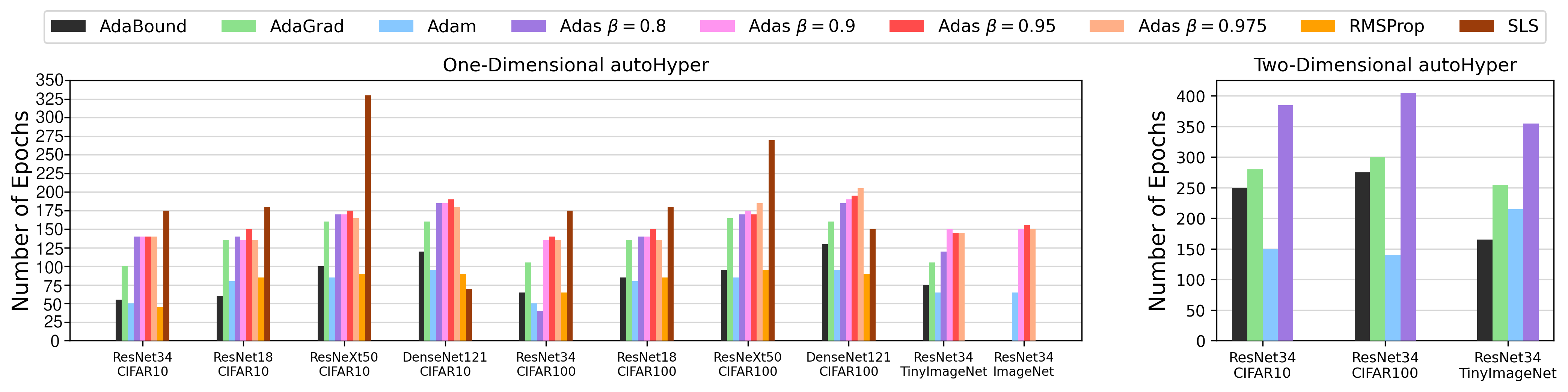
Figure 4: Required number of epochs for autoHyper to converge over various setups.

4 Experiments

4.1 Experimental Setups

One-dimensional comparison. We restrict our focus to the initial learning rate ($\lambda=\eta$) and run experiments on CIFAR10 (Krizhevsky et al., 2009), CIFAR100 (Krizhevsky et al., 2009), TinyImageNet (Li et al., ), and ImageNet (Russakovsky et al., 2015). On CIFAR10 and CIFAR100, we apply ResNet18 and ResNet34 (He et al., 2015), ResNeXt50 (Xie et al., 2016), and DenseNet121 (Huang et al., 2017). On TinyImageNet and ImageNet, we apply ResNet34. For architectures applied to CIFAR10 and CIFAR100, we train using Adam (Kingma and Ba, 2014), AdaBound (Luo et al., 2019), Adas^{($\beta=\{0.8,0.9,0.95,0.975\}$)} (Hosseini and Plataniotis, 2020) (with early-stop), AdaGrad (Duchi et al., 2011), RMSProp (Tieleman and Hinton, 2012), and SLS (Vaswani et al., 2019). For ResNet34 applied to TinyImageNet, we train using Adam, AdaBound, AdaGrad, and Adas^{($\beta=\{0.8,0.9,0.95,0.975\}$)}. For ResNet34 applied to ImageNet, we train using Adam and Adas^{($\beta=\{0.9,0.95,0.975\}$)}. Further, we conduct baselines using the author suggested learning rates, RS generated learning rates, and BO generated learning rates. Only Adam, AdaBound, AdaGrad, and Adas^$0.9$ are used in the RS and BO baselines. Each experiment is run for $5$ randomly initialized trials, each for 250 epochs, and we report averages.

Two-dimensional Comparison. We restrict our focus to the initial learning rate and weight decay rate ($\lambda=\{\eta,\gamma\}$) and run experiments on CIFAR10, CIFAR100, and TinyImageNet. We apply ResNet34 and train using Adam, AdaBound, AdaGrad, and Adas^$\beta=0.9$. Our baseline is composed only of BO generated initial learning rate and weight decay rate. Each experiment is run 5 times from randomly initialized starting points, each for 250 epochs, and we report averages.

Random Search and Bayesian Optimization setup. Because RS and BO are highly sensitive to the manually set search spaces (Choi et al., 2020; Sivaprasad et al., 2020), we attempt a fair comparison by providing similar search spaces that autoHyper is designed around. That is, for learning rate, $\eta_{min}=$1\text{\times}{10}^{-4}$$ and $\eta_{max}=0.1$ and for weight decay rate, $\gamma_{min}=$1\text{\times}{10}^{-7}$$ and $\gamma_{max}=0.1$. Both RS and BO are given the same computational budget that autoHyper had for each experiment (see Figure 4). This does provide the RS and BO experiments with a slight advantage since a priori knowledge of how many epochs and trials to consider is not provided to autoHyper. Further, RS and BO are given the advantage of using the test set for evaluation, since CIFAR10/CIFAR100 do not have an explicit development set. This was also done for TinyImageNet.

Additional notes. For BO, we used the Adaptive Experimentation Platform (https://ax.dev/ (Balandat et al., 2020)). Additional results and details are in Appendix-D and Appendix-E.

A note on multi-fidelity techniques. We attempted experiments on HyperBand Li et al. (2017) and BOHB Falkner et al. (2018) using the HPBandSter library but found that tuning the number of iterations (e.g. for successive halving) and the allocated budget to be difficult and iterative, and performance was significantly worse. For fairness, those experiments were not completed, as they required much more tuning.

4.2 Results

4.2.1 One-Dimensional Comparison

Consistency across experimental setup. Table 1 tells us that our method generalizes well to experimental setups. If there is loss of performance when using an initial learning rate generated by autoHyper, this loss is $<1\%$ in all experiments except three: On CIFAR100, the author baselines of ResNeXt50 trained using Adam, ResNext50 trained using RMSProp, and DenseNet121 trained using AdaBound achieve $1.2\%$, $2.28\%$ and $2.3\%$ better top-1 test accuracy, respectively.

Table 1: Final epoch (250) top-1 test accuracies for $\lambda=\eta$. Values marked with a ‘*’ indicate early-stopping. The best result is highlighted in green, and for autoHyper results, orange highlights when the results lie within the standard deviation from the best.

	ResNet34 on TinyImageNet				ResNet34 on CIFAR100
Optimizer	Author	RS	BO	autoHyper	Author	RS	BO	autoHyper
AdaBound	$55.48_{\pm 0.67}$	$54.88_{\pm 0.57}$	$55.18_{\pm 0.13}$	${\color[rgb]{0.0390625,0.58984375,0.0390625}\bm{56.22_{\pm 0.17}}}$	$71.94_{\pm 0.66}$	$73.17_{\pm 0.09}$	${\color[rgb]{0.0390625,0.58984375,0.0390625}\bm{73.34_{\pm 0.50}}}$	${\color[rgb]{1,0.55078125,0}\bm{73.15_{\pm 0.24}}}$
AdaGrad	${\color[rgb]{0.0390625,0.58984375,0.0390625}\bm{55.81_{\pm 0.84}}}$	$50.66_{\pm 0.33}$	$51.26_{\pm 0.55}$	${\color[rgb]{1,0.55078125,0}\bm{55.04_{\pm 0.54}}}$	$67.02_{\pm 0.23}$	$66.02_{\pm 0.59}$	$67.11_{\pm 0.54}$	${\color[rgb]{0.0390625,0.58984375,0.0390625}\bm{67.43_{\pm 0.59}}}$
Adam	$52.13_{\pm 1.14}$	$54.86_{\pm 0.21}$	${\color[rgb]{0.0390625,0.58984375,0.0390625}\bm{54.96_{\pm 0.39}}}$	${\color[rgb]{1,0.55078125,0}\bm{54.46_{\pm 1.14}}}$	$71.11_{\pm 0.37}$	$70.55_{\pm 0.15}$	$70.94_{\pm 0.62}$	${\color[rgb]{0.0390625,0.58984375,0.0390625}\bm{71.43_{\pm 0.28}}}$
Adas$0.9$	$59.91_{\pm 0.45}$	$59.76_{\pm 0.50}$	$59.52_{\pm 0.19}$	${\color[rgb]{0.0390625,0.58984375,0.0390625}\bm{61.56_{\pm 0.58}}}$	${\color[rgb]{0.0390625,0.58984375,0.0390625}\bm{75.99_{\pm 0.09}}}$	$73.51_{\pm 0.13}$	$69.38_{\pm 0.62}$	${\color[rgb]{1,0.55078125,0}\bm{75.78^{*}_{\pm 0.21}}}$
	ResNet18 on CIFAR100				DenseNet121 on CIFAR100
Optimizer	Author	RS	BO	autoHyper	Author	RS	BO	autoHyper
AdaBound	$72.04_{\pm 0.30}$	${\color[rgb]{0.0390625,0.58984375,0.0390625}\bm{73.24_{\pm 0.30}}}$	$73.28_{\pm 0.21}$	${\color[rgb]{1,0.55078125,0}\bm{\bm{73.16_{\pm 0.25}}}}$	$68.90_{\pm 0.36}$	${\color[rgb]{0.0390625,0.58984375,0.0390625}\bm{69.30_{\pm 0.22}}}$	$68.91_{\pm 0.23}$	$67.00_{\pm 0.20}$
AdaGrad	${\color[rgb]{0.0390625,0.58984375,0.0390625}\bm{67.76_{\pm 0.50}}}$	$67.75_{\pm 0.24}$	$67.40_{\pm 0.43}$	${\color[rgb]{1,0.55078125,0}\bm{67.75_{\pm 0.56}}}$	$62.14_{\pm 0.15}$	$62.43_{\pm 0.83}$	$62.57_{\pm 0.65}$	${\color[rgb]{0.0390625,0.58984375,0.0390625}\bm{62.79_{\pm 0.35}}}$
Adam	$70.34_{\pm 0.27}$	$70.58_{\pm 0.24}$	${\color[rgb]{0.0390625,0.58984375,0.0390625}\bm{71.03_{\pm 0.42}}}$	$70.09_{\pm 0.35}$	$67.48_{\pm 0.17}$	$67.96_{\pm 0.23}$	$68.58_{\pm 0.64}$	${\color[rgb]{0.0390625,0.58984375,0.0390625}\bm{69.05_{\pm 0.49}}}$
Adas$0.9$	$75.15_{\pm 0.17}$	$75.11_{\pm 0.18}$	$75.13_{\pm 0.23}$	${\color[rgb]{0.0390625,0.58984375,0.0390625}\bm{75.27^{*}_{\pm 0.28}}}$	${\color[rgb]{0.0390625,0.58984375,0.0390625}\bm{73.25_{\pm 0.25}}}$	$73.22_{\pm 0.30}$	$72.89_{\pm 0.20}$	${\color[rgb]{1,0.55078125,0}\bm{73.13^{*}_{\pm 0.44}}}$

Improved performance over RS and BO. We highlight how autoHyper is able to generalize over experimental setup whereas RS and BO cannot. In particular, RS and BO applied on AdaGrad and Adas^$0.9$ struggle to compete with autoHyper, particularly in more complex datasets such as CIFAR100. This is most evident in ResNet34 applied to CIFAR100 (see Table 1). This highlights how autoHyper can automatically find more competitive learning rates to RS and BO and without any manual intervention. Most interestingly, RS and BO were given a large advantage in that testing accuracy was used in their implementation rather than the conventional validation accuracy, and yet autoHyper’s performance (which uses training data) is maintained.

Table 2: ImageNet test accuracies for $\lambda=\eta$.

	ResNet34 on ImageNet
Method	Adam	Adas$0.9$	Adas$0.95$	Adas$0.975$
Author	$63.75_{\pm 0.08}$	${\color[rgb]{0.0390625,0.58984375,0.0390625}\bm{72.11_{\pm 0.16}}}$	$73.05_{\pm 0.17}$	${\color[rgb]{0.0390625,0.58984375,0.0390625}\bm{72.52_{\pm 0.03}}}$
autoHyper	${\color[rgb]{0.0390625,0.58984375,0.0390625}\bm{68.68_{\pm 0.24}}}$	${\color[rgb]{1,0.55078125,0}\bm{71.87^{*}_{\pm 0.20}}}$	${\color[rgb]{0.0390625,0.58984375,0.0390625}\bm{73.09_{\pm 0.23}}}$	${\color[rgb]{1,0.55078125,0}\bm{72.42_{\pm 0.15}}}$

ImageNet/TinyImageNet Improvements. We highlight how well autoHyper performs when applied to TinyImagetNet and ImageNet. ResNet34 trained using Adam and applied to TinyImageNet and ImageNet achieves final improvements of $3.14\%$ and $4.93\%$ in top-1 test accuracy, respectively, shown in Table 2. Such improvements come at a minimal cost using our method, requiring 65 epochs (4 hours) and 80 epochs (59 hours) for TinyImageNet and ImageNet, respectively (Figure 4).

Fast and consistent convergence rates. We visualize the convergence rates of our method in Figure 4. Importantly, we identify autoHyper’s consistency in required epochs per optimizer across architecture and dataset selection as well as the low convergence times. Our method exhibits less consistent results when optimizing using SLS as SLS tends to result in high ${\mathcal{Z}}(\eta)$ over multiple epochs and different learning rates. Despite this, our autoHyper still converges and performs well.

Table 3: Final epoch (250) top-1 test accuracies $\lambda=\{\eta,\gamma\}$.

	ResNet34 on TinyImageNet				ResNet34 on CIFAR10
Method	AdaBound	AdaGrad	Adam	Adas$0.9$	AdaBound	AdaGrad	Adam	Adas$0.9$
BO	$54.92_{\pm 0.30}$	$49.56_{\pm 0.54}$	$53.45_{\pm 0.56}$	$58.17_{\pm 0.32}$	${\color[rgb]{0.0390625,0.58984375,0.0390625}\bf{93.21_{\pm 0.16}}}$	$90.50_{\pm 0.16}$	$93.18_{\pm 0.25}$	$91.52_{\pm 0.08}$
autoHyper	${\color[rgb]{0.0390625,0.58984375,0.0390625}\bf{57.02_{\pm 0.20}}}$	${\color[rgb]{0.0390625,0.58984375,0.0390625}\bf{55.59_{\pm 0.71}}}$	${\color[rgb]{0.0390625,0.58984375,0.0390625}\bf{55.29_{\pm 0.20}}}$	${\color[rgb]{0.0390625,0.58984375,0.0390625}\bf{58.19_{\pm 0.20}}}$	${\color[rgb]{1,0.55078125,0}\bf{92.84_{\pm 0.28}}}$	${\color[rgb]{0.0390625,0.58984375,0.0390625}\bf{91.49_{\pm 0.21}}}$	${\color[rgb]{0.0390625,0.58984375,0.0390625}\bf{93.24_{\pm 0.06}}}$	${\color[rgb]{0.0390625,0.58984375,0.0390625}\bf{92.64_{\pm 0.18}}}$

4.2.2 Two-Dimensional Comparison

Improved performance over Bayesian Optimization. Analyzing Table 3, we see that autoHyper outperforms BO in the two-dimensional case. In particular, there is a $3.74\%$ improvement for ResNet34 applied to CIFAR100 using Adam. Of the $12$ experiments, there are only $3$ where BO is able to outperform autoHyper. We note that, of these $3$ cases, autoHyper is within the standard deviation of error in all but two: ResNet34 applied to CIFAR100 using AdaGrad and Adas^$0.9$.

Improvements in TinyImageNet. We highlight how autoHyper is able to significantly outperform BO on the more complex TinyImageNet dataset. In particular, ResNet34 applied to TinyImageNet, autoHyper achieves $2.1\%$, $6.03\%$, and $1.84\%$ improvement when using AdaBound, AdaGrad, and Adam, respectively. This result is very promising as complex datasets are often the most difficult and time consuming datasets to perform HPO on.

5 Conclusion

In this introductory work, we explored a new class of hyper-parameter optimization and proposed an analytical response surface that acts as a surrogate to validation metrics and generalizes well. We proposed an algorithm, autoHyper, that optimizes for this surface and progresses towards fully automatic multi-dimensional HPO. autoHyper is able to, on average, outperform existing SOTA and only requires training data. In future works, we would like to expand beyond the two-dimensional case and explore further developments to our metric. Further, we would like to research ways in eliminating the current internal hyper-parameters as well improvements in computational complexities, particularly when applied to the multi-dimensional case.

Appendix A Stable Rank Optimality

Given the definitions of stable rank in Equation 1 , we argue that a stable rank of $1$ indicates a perfectly learned network. Specifically, higher values ${\mathcal{G}}(\widehat{{\bm{\mathsfit{W}}}}_{d})\rightarrow 1$ indicates that most singular values are non-zero (i.e. $\sigma_{i}^{2}(\widehat{{\bm{\mathsfit{W}}}}_{d})>0\forall i\in[1,\ldots,n^{\prime}]$ where $n^{\prime}\rightarrow n$. This creates a subspace spanned by a set of independent vectors corresponding to the non-zero singular values mentioned above. In other words, ${\mathcal{G}}(\widehat{{\bm{\mathsfit{W}}}}_{d})\rightarrow 1$ corresponds to a many-to-many mapping but not a many-to-low (i.e. rank-deficient) mapping. Also, note that the stable rank is measured on the low-rank and not the raw measure of the weights. So the higher value indicates that the learned weight matrix contains more non-empty structure which can be interpreted as a sign of a meaningful learning.

Appendix B Rank behaviour over multiple epochs

Here we present the behaviour of ${\mathcal{Z}}_{t}(\eta)$.

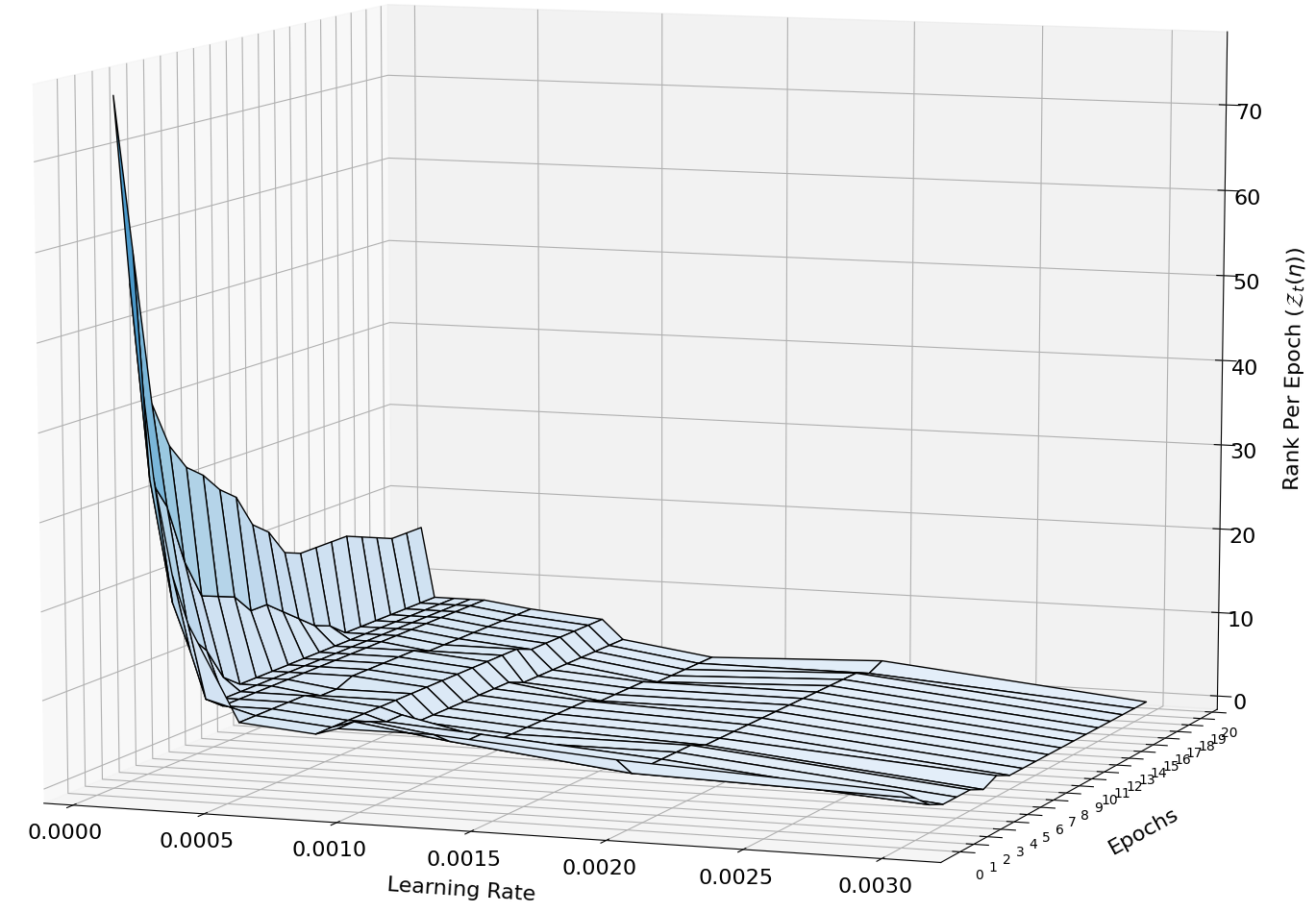
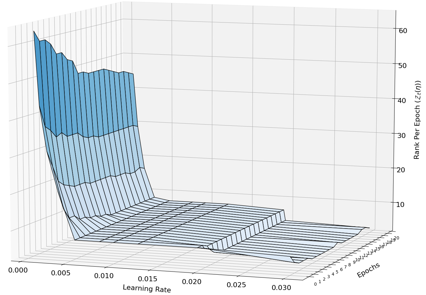
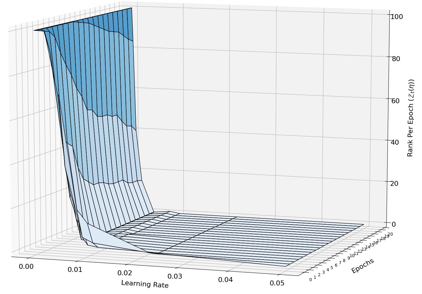
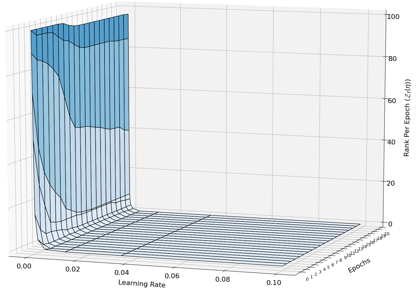
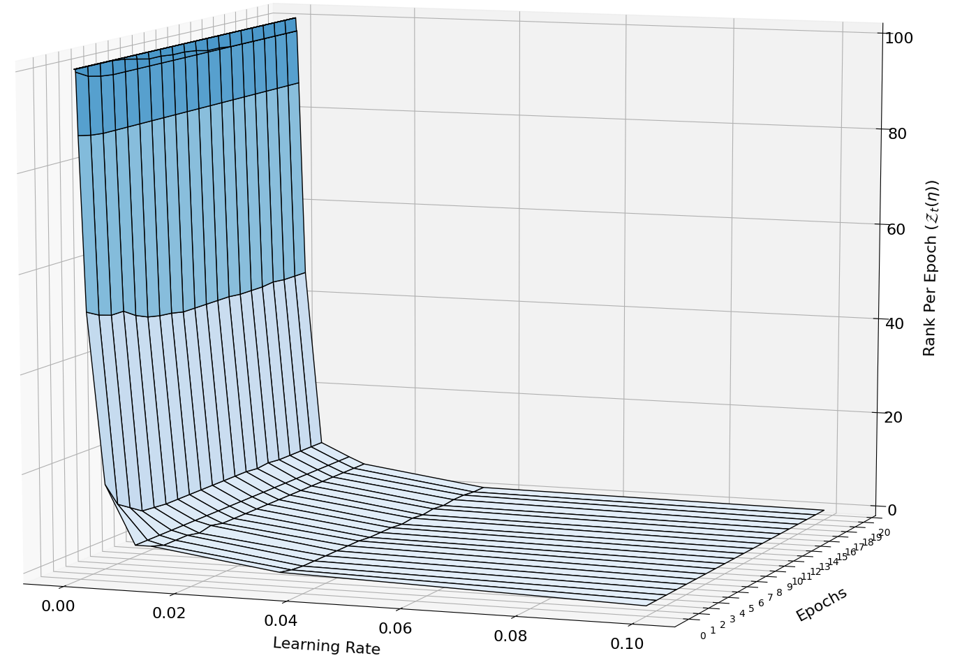
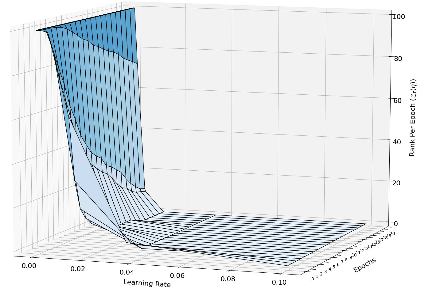
[Adam] [AdaGrad] [Adas $\beta=0.8$] [RMSProp]
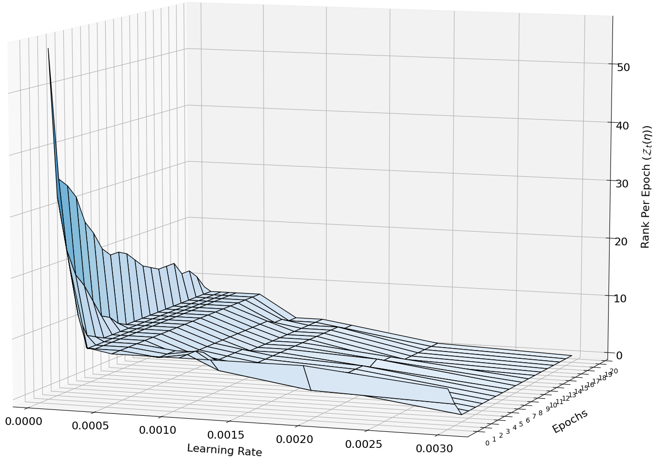
[Adam] [AdaGrad] [Adas $\beta=0.8$] [RMSProp]

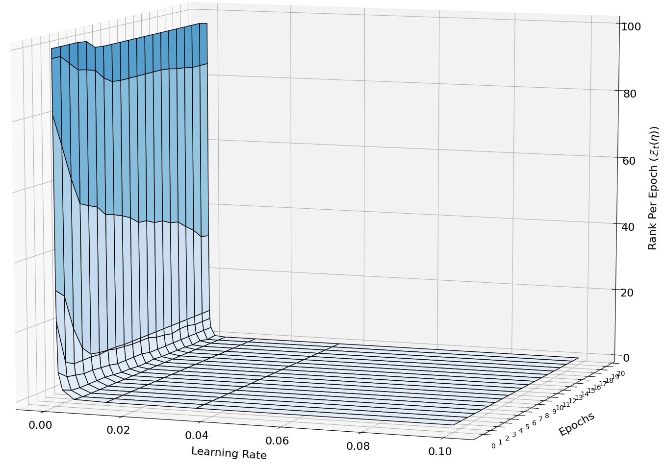
Figure B.1: Rank (${\mathcal{Z}}_{t}(\eta)$) for various learning rates on VGG16 trained using Adam, AdaGrad, Adas $\beta=0.8$, and RMSProp and applied to CIFAR10. A fixed epoch budget of 20 was used. We highlight how across these 20 epochs, very little progress is made beyond the first first epochs. It is from this analysis that we choose our epoch range of $T=5$.

Appendix C Additional Figures for Response Surface

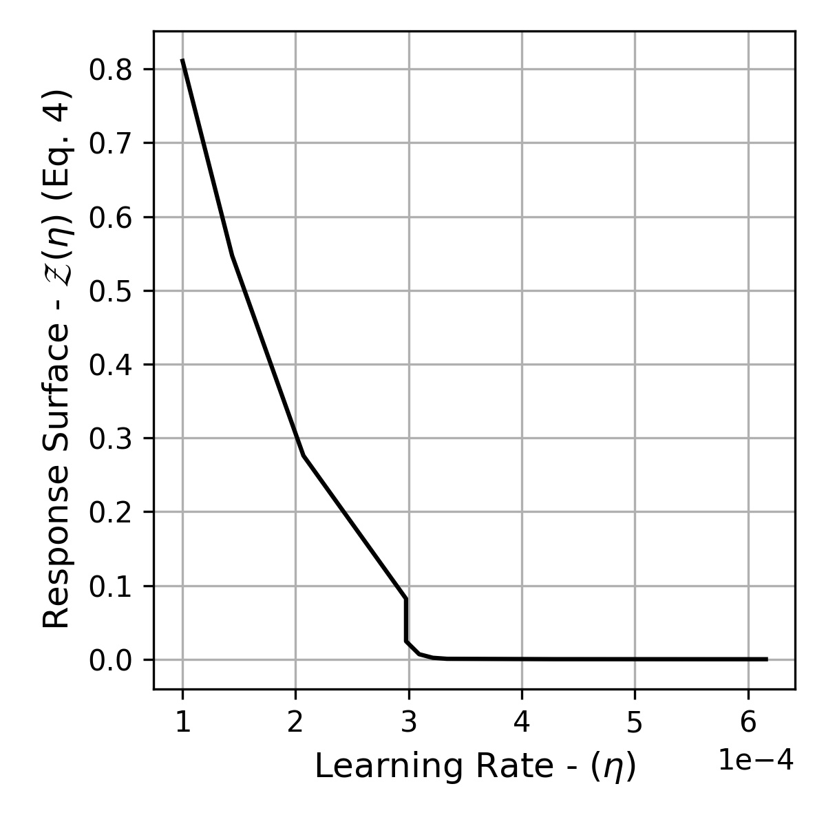
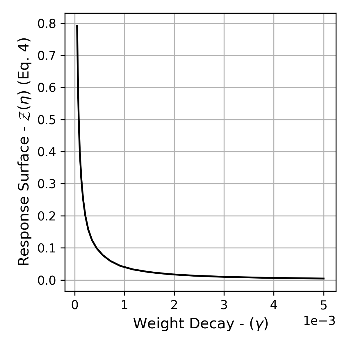
Figure C.2: Behaviour of our metric ${\mathcal{Z}}(\lambda)$ in response to initial learning rate and weight decay. Note that we plot the regularized cumulative product of ${\mathcal{Z}}(\lambda)$ here.

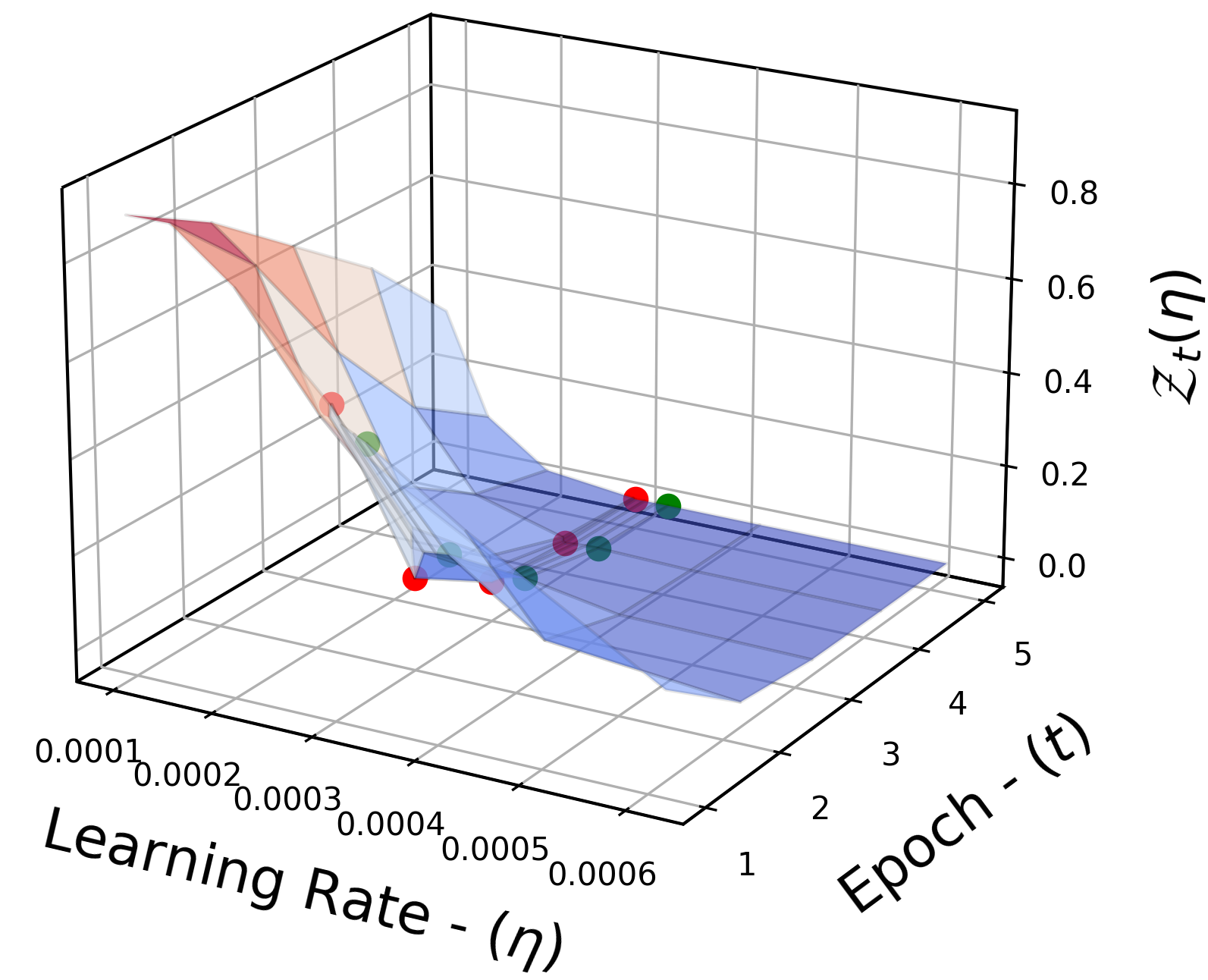
Figure C.3: ${\mathcal{Z}}_{t}(\eta)$ for various learning rates using Adam on ResNet34 applied to CIFAR10. The author-suggested initial learning rate is indicated by the red markers, and the autoHyper suggested learning rate is indicated by the green markers.

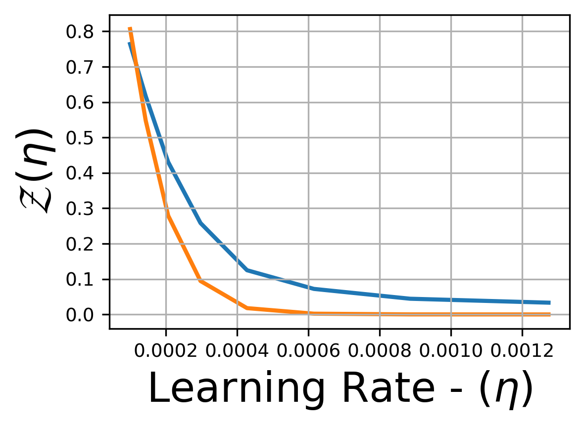
[ResNet34/Adam] [EffNetB0/Adas^$\beta=0.8$]

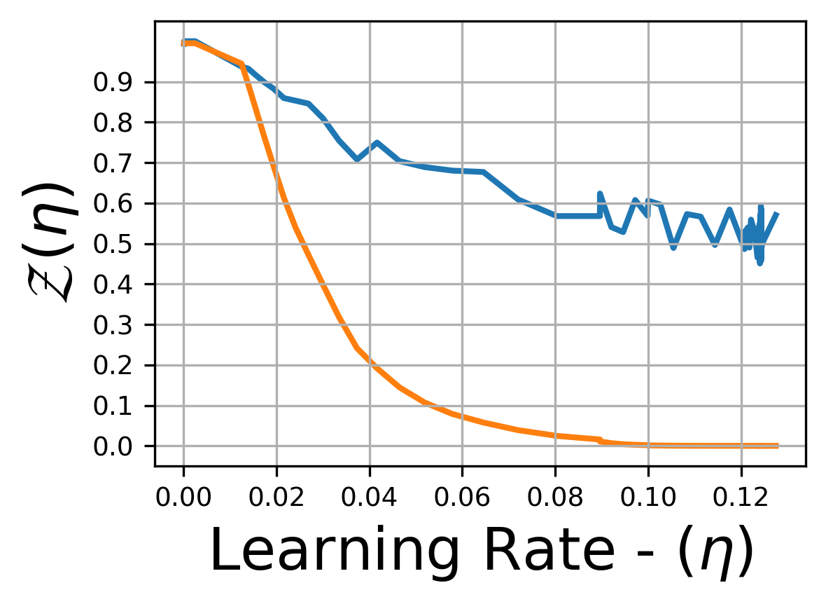
Figure C.4: ${\mathcal{Z}}(\eta)$ (blue) vs. cumprod(${\mathcal{Z}}(\eta)$)^0.8 (orange) for (a) a stable and (b) an unstable architecture on CIFAR10.

Appendix D Additional Experimental Details for Subsection 4.1

We note the additional configurations for our experimental setups.

Datasets: For CIFAR10 and CIFAR100, we perform random cropping to $32\times 32$ and random horizontal flipping on the training images and make no alterations to the test set. For TinyImageNet, we perform random resized cropping to $64\times 64$ and random horizontal flipping on the training images and center crop resizing to $64\times 64$ on the test set. For ImageNet, we follow He et al. (2015) and perform random resized cropping to $224\times 244$ and random horizontal flipping and $256\times 256$ resizing with $224\times 224$ center cropping on the test set.

Additional Configurations: Experiments on CIFAR10, CIFAR100, and TinyImageNet used mini-batch sizes of 128 and ImageNet experiments used mini-batch sizes of 256. For weight decay, $5\text{\times}{10}^{-4}$ was used for Adas-variants on CIFAR10 and CIFAR100 experiments and $1\text{\times}{10}^{-4}$ for all optimizers on TinyImageNet and ImageNet experiments, with the exception of Adam using a weight decay of $7.8125\text{\times}{10}^{-6}$. For Adas-variant, the momentum rate for momentum-SGD was set to $0.9$. All other hyper-parameters for each respective optimizer remained default as reported in their original papers. For author suggested learning rates, for CIFAR10 and CIFAR100, we use the manually tuned suggested learning rates as reported in Wilson et al. (2017) for Adam, RMSProp, and AdaGrad. For TinyImageNet and ImageNet, we use the suggested learning rates as reported in each optimizer’s respective paper. Refer to Tables 4-8 to see exactly which learning rates were used, as well as the learning rates generated by autoHyper. Further, see 8 for the learning rates and weight decay reates generated by BO and autoHyper. CIFAR10, CIFAR100, and TinyImageNet experiments were trained for 5 trials with a maximum of 250 epochs and ImageNet experiments were trained for 3 trials with a maximum of 150 epochs. Due to Adas’ stable test accuracy behaviour as demonstrated by Hosseini and Plataniotis (2020), an early-stop criteria, monitoring testing accuracy, was used for CIFAR10, CIFAR100, and ImageNet experiments. For CIFAR10 and CIFAR100, a threshold of $1\text{\times}{10}^{-3}$ for Adas^$\beta=0.8$ and $1\text{\times}{10}^{-4}$ for Adas^{$\beta=\{0.9,0.95\}$} and patience window of $10$ epochs. For ImageNet, a threshold of $1\text{\times}{10}^{-4}$ for Adas^{$\beta=\{0.8,0.9,0.95\}$} and patience window of $20$ epochs. No early stop is used for Adas^{$\beta=0.975$}.

Learning Rates: We report every learning rate in Tables 4-8.

Random Search: The search space is set to $[$1\text{\times}{10}^{-4}$,0.1]$ and a loguniform (see SciPy) distribution is used for sampling. This is motivated by the fact that autoHyper also uses and logarithmically-spaced grid space. We note that we ran initial tests against a uniform distribution for sampling was done and showed slightly worse results, as the favouring of smaller learning rates benefits the optimizers we considered. In keeping with autoHyper’s design, the learning rate that resulted in highest training accuracy after $5$ epochs was chosen. One could also track testing loss, however we found very little to no differences between the two in initial testing. Further work could include completing both testing loss and testing accuracy baselines, and picking the best one, however this is double the computational that autoHyper requires and therefore we deemed it not a fair comparison. Note also we used testing accuracy and not validation accuracy as is normally done, however this only benefits Random Search.

Bayesian Optimization: We used Facebook’s Adaptive Experimentation Platform (AX) to perform the Bayesian Optimization. In the background, AX uses Balandat et al. (2020), and we refer the reader to that paper for specific details. In keeping with Random Search as well as tutorials on the AX website, testing accuracy was used. Note also we used testing accuracy and not validation accuracy as is normally done, however this only benefits Bayesian Optimization.

Table 4: Learning Rates for ResNet34 applied to ImageNet

Optimizer	Author	autoHyper
Adam	$0.001$	$0.0001965$
Adas($0.9$)	$0.02$	$0.011479$
Adas($0.95$)	$0.02$	$0.011479$
Adas($0.975$)	$0.02$	$0.011479$

Table 5: Learning rates for ResNet34 applied to TinyImageNet. These are the one-dimensional hyper-parameter comparison values.

Optimizer	Author	RS	BO	autoHyper
AdaBound	1.00e-3	1.24e-4	1.64e-4	9.44e-5
AdaGrad	1.00e-2	7.15e-4	7.97e-4	2.24e-3
Adam	1.00e-3	1.75e-4	1.81e-4	1.96e-4
Adas$0.9$	3.00e-2	3.95e-2	6.76e-2	8.59e-3
Adas$0.8$	3.00e-2	-	-	1.01e-2
Adas$0.95$	3.00e-2	-	-	8.59e-3
Adas$0.975$	3.00e-2	-	-	8.59e-3

Table 6: Learning rates for various networks applied to CIFAR10 in the one-dimensional comparison.

(a) ResNet18
Optimizer	Author	RS	BO	autoHyper
AdaBound	1.00e-3	2.65e-4	2.55e-4	3.60e-4
AdaGrad	1.00e-2	2.13e-3	2.56e-3	4.97e-3
Adam	3.00e-4	1.45e-4	3.37e-4	6.76e-4
Adas$0.9$	3.00e-2	2.23e-2	2.60e-2	1.04e-2
Adas$0.8$	3.00e-2	-	-	1.27e-2
Adas$0.95$	3.00e-2	-	-	1.04e-2
Adas$0.975$	3.00e-2	-	-	1.04e-2
RMSProp	3.00e-4	-	-	4.70e-4
SLS	1.0	-	-	3.42e-2
(b) ResNet34
Optimizer	Author	RS	BO	autoHyper
AdaBound	1.00e-3	3.92e-4	5.47e-4	3.47e-4
AdaGrad	1.00e-2	1.60e-3	1.63e-3	2.86e-3
Adam	3.00e-4	3.30e-4	3.42e-4	3.34e-4
Adas$0.9$	3.00e-2	6.78e-3	4.32e-3	1.24e-2
Adas$0.8$	3.00e-2	-	-	1.24e-2
Adas$0.95$	3.00e-2	-	-	1.24e-2
Adas$0.975$	3.00e-2	-	-	1.24e-2
RMSProp	3.00e-4	-	-	1.68e-4
SLS	1.0	-	-	3.42e-2
(c) ResNeXt50
Optimizer	Author	RS	BO	autoHyper
AdaBound	1.00e-3	1.87e-4	4.79e-4	9.72e-4
AdaGrad	1.00e-2	3.80e-3	4.96e-3	8.97e-3
Adam	3.00e-4	1.48e-4	2.82e-4	9.72e-4
Adas$0.9$	3.00e-2	1.38e-2	1.86e-2	2.32e-2
Adas$0.8$	3.00e-2	-	-	1.27e-2
Adas$0.95$	3.00e-2	-	-	2.31e-2
Adas$0.975$	3.00e-2	-	-	1.04e-2
RMSProp	3.00e-4	-	-	4.70e-4
SLS	1.0	-	-	3.42e-2
(d) DenseNet121
Optimizer	Author	RS	BO	autoHyper
AdaBound	1.00e-3	8.91e-4	9.21e-4	3.02e-3
AdaGrad	1.00e-2	4.85e-3	8.37e-3	1.54e-2
Adam	3.00e-4	7.50e-4	4.81e-4	2.01e-3
Adas$0.9$	3.00e-2	2.09e-2	3.07e-2	5.98e-2
Adas$0.8$	3.00e-2	-	-	6.10e-2
Adas$0.95$	3.00e-2	-	-	4.92e-2
Adas$0.975$	3.00e-2	-	-	5.98e-2
RMSProp	3.00e-4	-	-	2.01e-3
SLS	1.0	-	-	3.12e-3

Table 7: Learning rates for various networks applied to CIFAR100 in the one-dimensional comparison.

(a) ResNet18
Optimizer	Author	RS	BO	autoHyper
AdaBound	1.00e-3	3.43e-4	2.92e-4	2.49e-4
AdaGrad	1.00e-2	4.51e-3	2.87e-3	4.97e-3
Adam	3.00e-4	3.59e-4	2.87e-4	6.76e-4
Adas$0.9$	3.00e-2	5.52e-2	3.06e-2	1.27e-2
Adas$0.8$	3.00e-2	-	-	1.27e-2
Adas$0.95$	3.00e-2	-	-	1.04e-2
Adas$0.975$	3.00e-2	-	-	7.07e-3
RMSProp	3.00e-4	-	-	4.70e-4
SLS	1.0	-	-	3.42e-2
(b) ResNet34
Optimizer	Author	RS	BO	autoHyper
AdaBound	1.00e-3	3.53e-4	1.76e-4	3.47e-4
AdaGrad	1.00e-2	1.83e-3	2.35e-3	2.24e-3
Adam	3.00e-4	1.25e-4	2.42e-4	2.41e-4
Adas$0.9$	3.00e-2	9.25e-3	2.14e-3	1.02e-2
Adas$0.8$	3.00e-2	-	-	1.03e-2
Adas$0.95$	3.00e-2	-	-	1.50e-2
Adas$0.975$	3.00e-2	-	-	1.02e-2
RMSProp	3.00e-4	-	-	1.97e-4
SLS	1.0	-	-	3.42e-2
(c) ResNeXt50
Optimizer	Author	RS	BO	autoHyper
AdaBound	1.00e-3	3.69e-4	5.03e-4	9.72e-4
AdaGrad	1.00e-2	2.74e-3	5.86e-3	1.19e-2
Adam	3.00e-4	4.38e-4	5.44e-4	9.72e-4
Adas$0.9$	3.00e-2	1.16e-2	1.26e-2	2.75e-2
Adas$0.8$	3.00e-2	-	-	1.27e-2
Adas$0.95$	3.00e-2	-	-	2.27e-2
Adas$0.975$	3.00e-2	-	-	7.0e-3
RMSProp	3.00e-4	-	-	4.70e-4
SLS	1.0	-	-	3.42e-2
(d) DenseNet121
Optimizer	Author	RS	BO	autoHyper
AdaBound	1.00e-3	8.91e-4	9.21e-4	3.02e-3
AdaGrad	1.00e-2	4.85e-3	8.37e-3	1.54e-2
Adam	3.00e-4	7.50e-4	4.81e-4	2.01e-3
Adas$0.9$	3.00e-2	2.09e-2	3.07e-2	5.98e-2
Adas$0.8$	3.00e-2	-	-	3.98e-2
Adas$0.95$	3.00e-2	-	-	3.57e-2
Adas$0.975$	3.00e-2	-	-	5.04e-2
RMSProp	3.00e-4	-	-	6.76e-2
SLS	1.0	-	-	8.79e-2

Table 8: Learning rates for ResNet34 applied to various dataset for the two-dimensional comparison.

(a) TinyImageNet
Optimizer	BO		autoHyper
	LR ($\eta$)	WD ($\gamma$)	LR ($\eta$)	WD ($\gamma$)
AdaBound	5.33e-5	6.28e-4	1.62e-5	7.17e-8
AdaGrad	5.21e-4	1.27e-3	4.27e-3	1.04e-7
Adam	7.03e-4	5.50e-6	2.19e-4	1.00e-7
Adas$0.9$	8.99e-3	1.05e-6	1.89e-2	9.67e-7
(b) CIFAR10
Optimizer	BO		autoHyper
	LR ($\eta$)	WD ($\gamma$)	LR ($\eta$)	WD ($\gamma$)
AdaBound	9.66e-6	4.32e-6	6.67e-4	3.41e-8
AdaGrad	2.92e-3	3.29e-5	6.20e-3	3.17e-7
Adam	4.35e-4	1.68e-8	6.67e-4	1.00e-7
Adas$0.9$	2.86e-3	1.87e-6	2.74e-2	6.43e-7
(c) CIFAR100
Optimizer	BO		autoHyper
	LR ($\eta$)	WD ($\gamma$)	LR ($\eta$)	WD ($\gamma$)
AdaBound	1.19e-5	5.73e-7	3.67e-6	2.35e-8
AdaGrad	4.08e-3	1.03e-3	6.20e-3	1.51e-7
Adam	1.52e-3	1.01e-6	4.60e-4	7.17e-8
Adas$0.9$	7.70e-3	1.12e-7	2.74e-2	4.60e-7

Appendix E Additional Results for Subsection 4.2

Table 9: Final epoch (250) top-1 test accuracies average over each trial for one-dimensional search ($\lambda=\eta$). Values marked with a ‘*’ indicate early-stopping. The best result is highlighted in green, and for autoHyper results, orange highlights when the results lie with the standard deviation from the best.

(a) ResNet34 on TinyImageNet
Optimizer	Author	RS	BO	autoHyper
Adas$0.8$	$57.98_{\pm 0.44}$	-	-	${\color[rgb]{0.0390625,0.58984375,0.0390625}\bm{58.02_{\pm 0.42}}}$
Adas$0.95$	$60.74_{\pm 0.20}$	-	-	${\color[rgb]{0.0390625,0.58984375,0.0390625}\bm{62.28_{\pm 0.44}}}$
Adas$0.975$	$61.44_{\pm 0.27}$	-	-	${\color[rgb]{0.0390625,0.58984375,0.0390625}\bm{61.81_{\pm 0.45}}}$
(c) ResNet34 on CIFAR10
Optimizer	Author	RS	BO	autoHyper
Adas$0.8$	$93.02_{\pm 0.13}$	-	-	${\color[rgb]{0.0390625,0.58984375,0.0390625}\bm{93.40^{*}_{\pm 0.15}}}$
Adas$0.95$	${\color[rgb]{0.0390625,0.58984375,0.0390625}\bm{95.20_{\pm 0.11}}}$	-	-	${\color[rgb]{1,0.55078125,0}\bm{95.08^{*}_{\pm 0.18}}}$
Adas$0.975$	${\color[rgb]{0.0390625,0.58984375,0.0390625}\bm{95.24_{\pm 0.15}}}$	-	-	${\color[rgb]{1,0.55078125,0}\bm{95.13_{\pm 0.11}}}$
RMSProp	$92.90_{\pm 0.29}$	-	-	${\color[rgb]{0.0390625,0.58984375,0.0390625}\bm{93.03_{\pm 0.23}}}$
SLS	${\color[rgb]{0.0390625,0.58984375,0.0390625}\bm{93.45_{\pm 0.16}}}$	-	-	${\color[rgb]{1,0.55078125,0}\bm{93.33_{\pm 0.06}}}$
(d) ResNet34 on CIFAR100
Optimizer	Author	RS	BO	autoHyper
Adas$0.8$	${\color[rgb]{0.0390625,0.58984375,0.0390625}\bm{74.21_{\pm 0.26}}}$	-	-	$73.58^{*}_{\pm 0.36}$
Adas$0.95$	${\color[rgb]{0.0390625,0.58984375,0.0390625}\bm{77.60_{\pm 0.22}}}$	-	-	${\color[rgb]{1,0.55078125,0}\bm{77.48^{*}_{\pm 0.37}}}$
Adas$0.975$	$78.00_{\pm 0.28}$	-	-	${\color[rgb]{0.0390625,0.58984375,0.0390625}\bm{78.26_{\pm 0.35}}}$
RMSProp	$70.25_{\pm 0.29}$	-	-	${\color[rgb]{0.0390625,0.58984375,0.0390625}\bm{70.57_{\pm 0.40}}}$
SLS	$73.22_{\pm 0.11}$	-	-	${\color[rgb]{0.0390625,0.58984375,0.0390625}\bm{73.77_{\pm 0.12}}}$
(e) ResNet18 on CIFAR10
Optimizer	Author	RS	BO	autoHyper
AdaBound	$92.35_{\pm 0.18}$	$92.64_{\pm 0.21}$	${\color[rgb]{0.0390625,0.58984375,0.0390625}{\color[rgb]{0.0390625,0.58984375,0.0390625}\bm{93.15_{\pm 0.11}}}}$	$92.85_{\pm 0.06}$
AdaGrad	${\color[rgb]{0.0390625,0.58984375,0.0390625}\bm{91.23_{\pm 0.25}}}$	$89.71_{\pm 0.18}$	$90.00_{\pm 0.08}$	${\color[rgb]{1,0.55078125,0}\bm{90.87_{\pm 0.14}}}$
Adam	$92.93_{\pm 0.22}$	$92.59_{\pm 0.05}$	$92.92_{\pm 0.18}$	${\color[rgb]{0.0390625,0.58984375,0.0390625}\bm{92.95_{\pm 0.24}}}$
Adas$0.9$	${\color[rgb]{0.0390625,0.58984375,0.0390625}\bm{94.05_{\pm 0.10}}}$	$94.11_{\pm 0.13}$	$94.01_{\pm 0.05}$	$93.75^{*}_{\pm 0.12}$
Adas$0.8$	${\color[rgb]{0.0390625,0.58984375,0.0390625}\bm{92.92_{\pm 0.19}}}$	-	-	${\color[rgb]{1,0.55078125,0}\bm{92.80^{*}_{\pm 0.16}}}$
Adas$0.95$	${\color[rgb]{0.0390625,0.58984375,0.0390625}\bm{94.93_{\pm 0.11}}}$	-	-	${\color[rgb]{1,0.55078125,0}\bm{94.74^{*}_{\pm 0.16}}}$
Adas$0.975$	${\color[rgb]{0.0390625,0.58984375,0.0390625}\bm{95.14_{\pm 0.20}}}$	-	-	${\color[rgb]{1,0.55078125,0}\bm{94.94_{\pm 0.04}}}$
RMSProp	$92.62_{\pm 0.30}$	-	-	${\color[rgb]{0.0390625,0.58984375,0.0390625}\bm{92.69_{\pm 0.33}}}$
SLS	${\color[rgb]{0.0390625,0.58984375,0.0390625}\bm{93.45_{\pm 0.16}}}$	-	-	${\color[rgb]{1,0.55078125,0}\bm{93.33_{\pm 0.06}}}$
(f) ResNet18 on CIFAR100
Optimizer	Author	RS	BO	autoHyper
Adas$0.8$	${\color[rgb]{0.0390625,0.58984375,0.0390625}\bm{73.59_{\pm 0.09}}}$	-	-	${\color[rgb]{1,0.55078125,0}\bm{73.38^{*}_{\pm 0.28}}}$
Adas$0.95$	${\color[rgb]{0.0390625,0.58984375,0.0390625}\bm{76.53_{\pm 0.30}}}$	-	-	${\color[rgb]{1,0.55078125,0}\bm{76.49^{*}_{\pm 0.37}}}$
Adas$0.975$	${\color[rgb]{0.0390625,0.58984375,0.0390625}\bm{77.23_{\pm 0.09}}}$	-	-	$76.68_{\pm 0.18}$
RMSProp	${\color[rgb]{0.0390625,0.58984375,0.0390625}\bm{70.08_{\pm 0.23}}}$	-	-	${\color[rgb]{1,0.55078125,0}\bm{69.28_{\pm 0.50}}}$
SLS	$73.22_{\pm 0.11}$	-	-	${\color[rgb]{0.0390625,0.58984375,0.0390625}\bm{73.77_{\pm 0.12}}}$

Table 10: Final epoch (250) top-1 test accuracies average over each trial for one-dimensional search ($\lambda=\eta$). Values marked with a ‘*’ indicate early-stopping. The best result is highlighted in green, and for autoHyper results, orange highlights when the results lie with the standard deviation from the best.

(g) ResNeXt50 on CIFAR10
Optimizer	Author	RS	BO	autoHyper
AdaBound	$91.42_{\pm 0.42}$	${\color[rgb]{0.0390625,0.58984375,0.0390625}\bm{92.37_{\pm 0.19}}}$	$92.10_{\pm 0.19}$	$91.69_{\pm 0.33}$
AdaGrad	$90.07_{\pm 0.27}$	$89.02_{\pm 0.23}$	$89.26_{\pm 0.26}$	${\color[rgb]{0.0390625,0.58984375,0.0390625}\bm{90.13_{\pm 0.19}}}$
Adam	$92.18_{\pm 0.31}$	$91.90_{\pm 0.17}$	${\color[rgb]{0.0390625,0.58984375,0.0390625}\bm{92.29_{\pm 0.33}}}$	${\color[rgb]{1,0.55078125,0}\bm{92.12_{\pm 0.07}}}$
Adas$0.9$	${\color[rgb]{0.0390625,0.58984375,0.0390625}\bm{93.60_{\pm 0.16}}}$	$93.51_{\pm 0.12}$	$93.39_{\pm 0.12}$	${\color[rgb]{1,0.55078125,0}\bm{93.51^{*}_{\pm 0.12}}}$
Adas$0.8$	${\color[rgb]{0.0390625,0.58984375,0.0390625}\bm{91.56_{\pm 0.07}}}$	-	-	${\color[rgb]{1,0.55078125,0}\bm{91.49^{*}_{\pm 0.16}}}$
Adas$0.95$	${\color[rgb]{0.0390625,0.58984375,0.0390625}\bm{94.62_{\pm 0.10}}}$	-	-	${\color[rgb]{1,0.55078125,0}\bm{94.61^{*}_{\pm 0.11}}}$
Adas$0.975$	${\color[rgb]{0.0390625,0.58984375,0.0390625}\bm{95.03_{\pm 0.12}}}$	-	-	${\color[rgb]{1,0.55078125,0}\bm{95.02_{\pm 0.06}}}$
RMSProp	${\color[rgb]{0.0390625,0.58984375,0.0390625}\bm{92.15_{\pm 0.20}}}$	-	-	$91.34_{\pm 0.59}$
SLS	$93.49_{\pm 0.14}$	-	-	${\color[rgb]{0.0390625,0.58984375,0.0390625}\bm{93.56_{\pm 0.20}}}$
(h) ResNeXt50 on CIFAR100
Optimizer	Author	RS	BO	autoHyper
AdaBound	$71.43_{\pm 0.30}$	${\color[rgb]{0.0390625,0.58984375,0.0390625}\bm{72.50_{\pm 0.28}}}$	$72.27_{\pm 0.30}$	${\color[rgb]{1,0.55078125,0}\bm{71.20_{\pm 0.34}}}$
AdaGrad	$65.66_{\pm 0.36}$	$62.32_{\pm 0.15}$	${\color[rgb]{0.0390625,0.58984375,0.0390625}\bm{66.07_{\pm 0.38}}}$	${\color[rgb]{1,0.55078125,0}\bm{66.03_{\pm 0.56}}}$
Adam	$70.32_{\pm 0.46}$	${\color[rgb]{0.0390625,0.58984375,0.0390625}\bm{70.33_{\pm 0.36}}}$	$69.95_{\pm 0.40}$	$69.12_{\pm 0.16}$
Adas$0.9$	${\color[rgb]{0.0390625,0.58984375,0.0390625}\bm{74.43_{\pm 0.14}}}$	$73.75_{\pm 0.30}$	$73.97_{\pm 0.16}$	${\color[rgb]{1,0.55078125,0}\bm{74.41^{*}_{\pm 0.26}}}$
Adas$0.8$	${\color[rgb]{0.0390625,0.58984375,0.0390625}\bm{72.41_{\pm 0.16}}}$	-	-	${\color[rgb]{1,0.55078125,0}\bm{72.00^{*}_{\pm 0.44}}}$
Adas$0.95$	${\color[rgb]{0.0390625,0.58984375,0.0390625}\bm{75.95_{\pm 0.26}}}$	-	-	${\color[rgb]{1,0.55078125,0}\bm{75.63^{*}_{\pm 0.12}}}$
Adas$0.975$	$76.46_{\pm 0.24}$	-	-	${\color[rgb]{0.0390625,0.58984375,0.0390625}\bm{76.58_{\pm 0.21}}}$
RMSProp	${\color[rgb]{0.0390625,0.58984375,0.0390625}\bm{69.45_{\pm 1.17}}}$	-	-	$67.17_{\pm 0.70}$
SLS	${\color[rgb]{0.0390625,0.58984375,0.0390625}\bm{72.08_{\pm 0.43}}}$	-	-	${\color[rgb]{1,0.55078125,0}\bm{71.82_{\pm 0.22}}}$
(i) DenseNet121 on CIFAR10
Optimizer	Author	RS	BO	autoHyper
Adas$0.8$	$91.28_{\pm 0.23}$	-	-	${\color[rgb]{0.0390625,0.58984375,0.0390625}\bm{91.59^{*}_{\pm 0.25}}}$
Adas$0.95$	${\color[rgb]{0.0390625,0.58984375,0.0390625}\bm{93.51_{\pm 0.20}}}$	-	-	${\color[rgb]{1,0.55078125,0}\bm{93.33^{*}_{\pm 0.24}}}$
Adas$0.975$	${\color[rgb]{0.0390625,0.58984375,0.0390625}\bm{93.83_{\pm 0.20}}}$	-	-	${\color[rgb]{0.0390625,0.58984375,0.0390625}\bm{93.47_{\pm 0.24}}}$
RMSProp	$91.29_{\pm 0.20}$	-	-	${\color[rgb]{0.0390625,0.58984375,0.0390625}\bm{91.83_{\pm 0.30}}}$
SLS	$93.16_{\pm 0.13}$	-	-	${\color[rgb]{0.0390625,0.58984375,0.0390625}\bm{93.36_{\pm 0.18}}}$
(j) DenseNet121 on CIFAR100
Optimizer	Author	RS	BO	autoHyper
Adas$0.8$	$70.63_{\pm 0.33}$	-	-	${\color[rgb]{0.0390625,0.58984375,0.0390625}\bm{71.01^{*}_{\pm 0.28}}}$
Adas$0.95$	${\color[rgb]{0.0390625,0.58984375,0.0390625}\bm{74.22_{\pm 0.24}}}$	-	-	${\color[rgb]{1,0.55078125,0}\bm{73.98^{*}_{\pm 0.33}}}$
Adas$0.975$	${\color[rgb]{0.0390625,0.58984375,0.0390625}\bm{74.10_{\pm 0.47}}}$	-	-	${\color[rgb]{1,0.55078125,0}\bm{7}3.97_{\pm 0.36}}$
RMSProp	$66.61_{\pm 0.58}$	-	-	${\color[rgb]{0.0390625,0.58984375,0.0390625}\bm{68.13_{\pm 0.00}}}$
SLS	$69.44_{\pm 0.61}$	-	-	${\color[rgb]{0.0390625,0.58984375,0.0390625}\bm{70.25_{\pm 0.19}}}$

[]

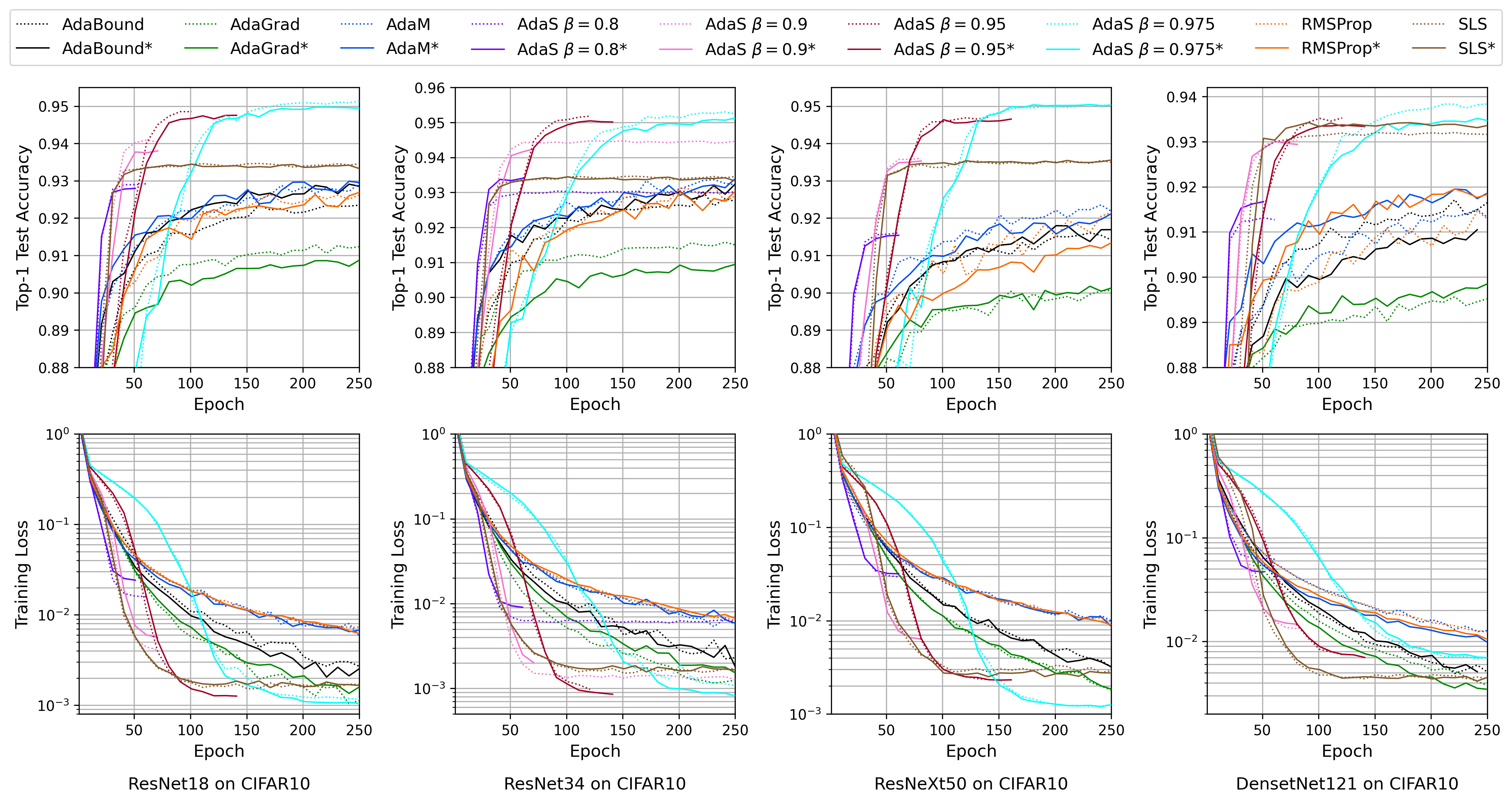
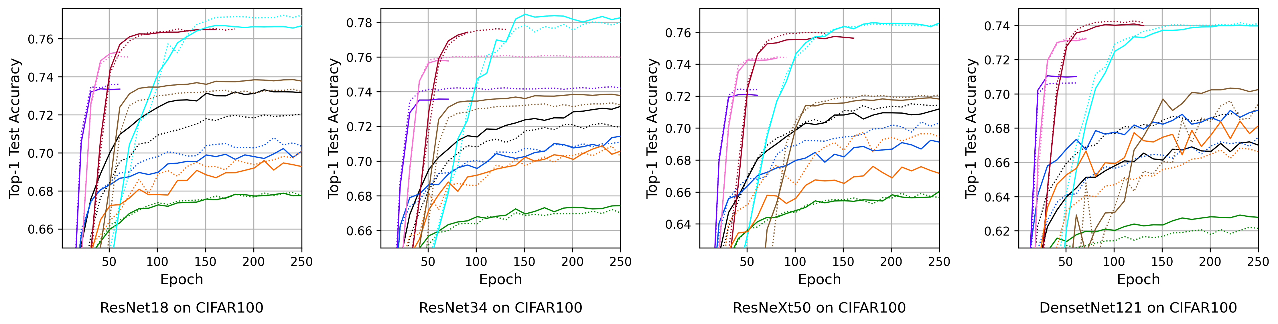
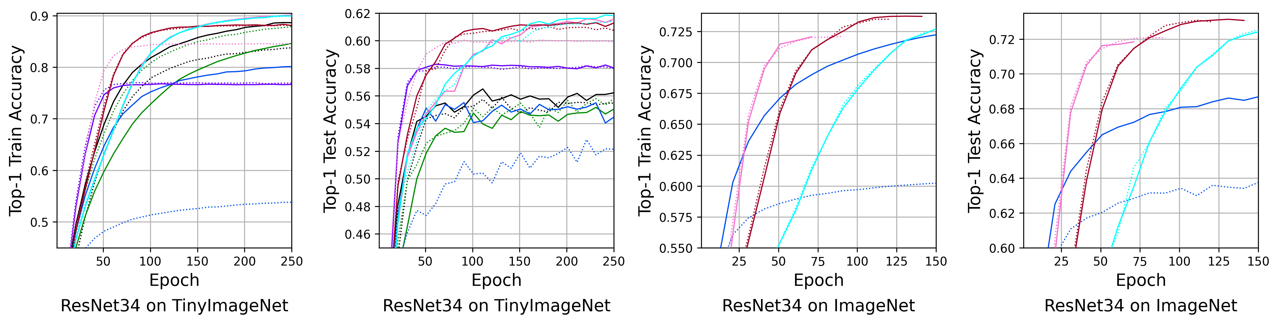
Figure E.5: Results of the (a) ablative study and (b) Random Search comparison experiments. Titles below plots indicate what experiment the above plots refers to. Legend labels marked by ‘*’ (solid lines) show results for autoHyper generated learning rates and dotted lines are the (a) baselines and (b) Random Search results.

Figure E.6: Test accuracy and trianing loss for EfficientNetB0 applied to CIFAR100. Importantly, EfficientNetB0 is an unstable network architecture in relation to our response surface and yet our method, autoHyper, is still able to converge and achieve competitive performance.

Figure E.7: Demonstration of the importance of initial learning rate in scheduled learning rate case, for ResNet18 applied on CIFAR10, using Step-Decay method with step-size = 25 epochs and decay rate = 0.5. As before, the dotted line represents the baseline results, with initial learning rate = 0.1, and the solid line represents the results using autoHyper’s suggested learning rate of 0.008585. These results highlight the importance of initial learning rate, even when using a scheduled learning rate heuristic, and demonstrates the importance of the additional step-size and decay rate hyper-parameters. Despite better initial performance from the autoHyper suggest learning rate, the step-size and decay rate choice cause the performance to plateau too early.

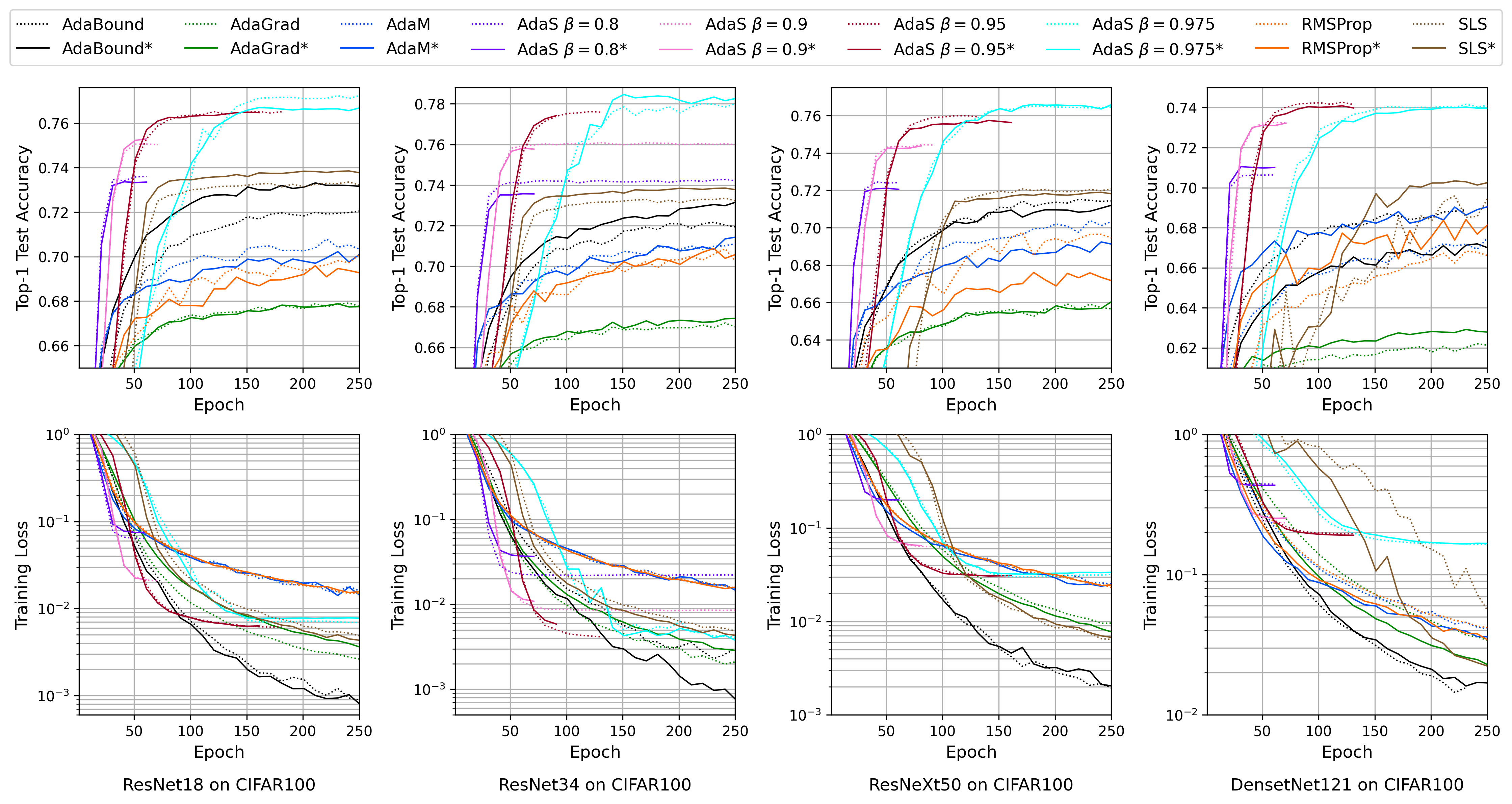
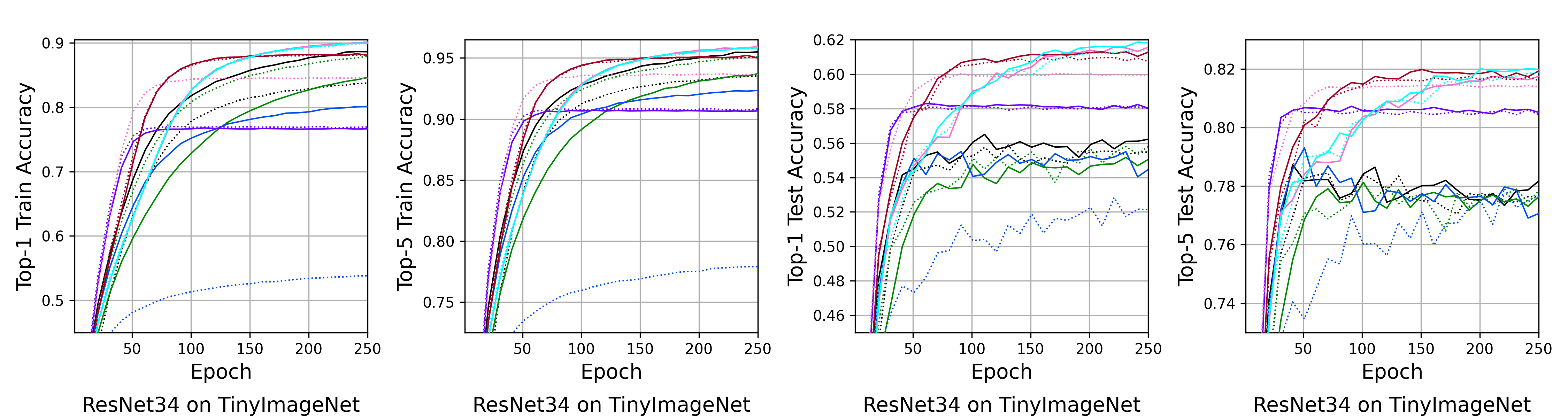
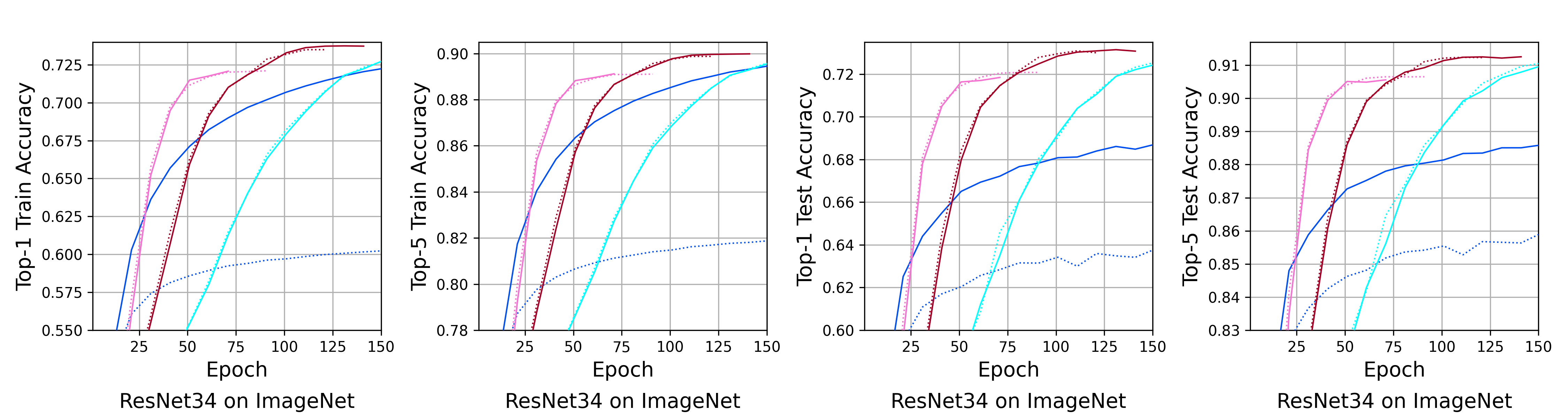
Figure E.8: Full results of CIFAR100, TinyImageNet, and ImageNet experiments. Top-1 test accuracy and training losses are reported for CIFAR100 experiments and top-1 and top-5 test and training accuracies are reported for TinyImageNet and ImageNet. Titles below the figures indicate to which experiments the above figures belong to. As before, lines indicated by the ‘*’ (solid lines), are results using initial learning rate as suggested by autoHyper.

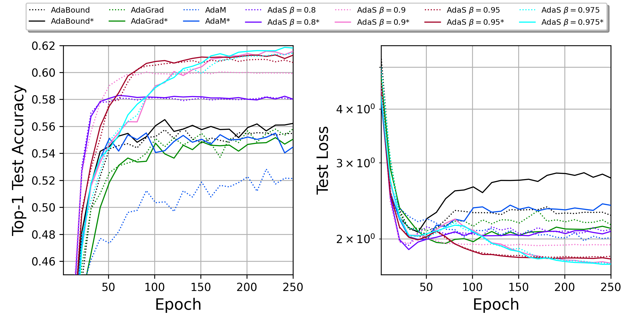
Figure E.9: Top-1 Test Accuracy and Test Loss for ResNet34 Experiments applied on TinyImageNet. As before, lines indicated by the ‘*’ (solid lines), are results using initial learning rate as suggested by autoHyper. These results visualize the inconsistency in tracking test loss as a metric to optimize final testing accuracy. This can be seen, for example, when looking at the test loss and test accuracy plots for Adam, where the test loss for the baseline is lower than that of the autoHyper suggested results but autoHyper achieves better test accuracy. These results also highlight the instability of tracking testing accuracy or less instead of the metric defined in Equation 5.

References

- Balandat et al. (2020) Maximilian Balandat, Brian Karrer, Daniel R. Jiang, Samuel Daulton, Benjamin Letham, Andrew Gordon Wilson, and Eytan Bakshy. BoTorch: A Framework for Efficient Monte-Carlo Bayesian Optimization. In Advances in Neural Information Processing Systems 33, 2020. URL https://proceedings.neurips.cc/paper/2020/hash/f5b1b89d98b7286673128a5fb112cb9a-Abstract.html.
- Bergstra and Bengio (2012) James Bergstra and Yoshua Bengio. Random search for hyper-parameter optimization. The Journal of Machine Learning Research, 13(1):281–305, 2012.
- Choi et al. (2020) Dami Choi, Christopher J. Shallue, Zachary Nado, Jaehoon Lee, Chris J. Maddison, and George E. Dahl. On empirical comparisons of optimizers for deep learning, 2020.
- Duchi et al. (2011) John Duchi, Elad Hazan, and Yoram Singer. Adaptive subgradient methods for online learning and stochastic optimization. Journal of machine learning research, 12(7), 2011.
- Falkner et al. (2018) Stefan Falkner, Aaron Klein, and Frank Hutter. Bohb: Robust and efficient hyperparameter optimization at scale, 2018.
- He et al. (2015) Kaiming He, Xiangyu Zhang, Shaoqing Ren, and Jian Sun. Deep residual learning for image recognition, 2015.
- Hosseini and Plataniotis (2020) Mahdi S. Hosseini and Konstantinos N. Plataniotis. Adas: Adaptive scheduling of stochastic gradients, 2020.
- Hosseini et al. (2021) Mahdi S Hosseini, Jia Shu Zhang, Zhe Liu, Andre Fu, Jingxuan Su, Mathieu Tuli, and Konstantinos N Plataniotis. Conet: Channel optimization for convolutional neural networks. In Proceedings of the IEEE/CVF International Conference on Computer Vision, pages 326–335, 2021.
- Huang et al. (2017) Gao Huang, Zhuang Liu, Laurens Van Der Maaten, and Kilian Q Weinberger. Densely connected convolutional networks. In Proceedings of the IEEE conference on computer vision and pattern recognition, pages 4700–4708, 2017.
- Jaegerman et al. (2021) Jonathan Jaegerman, Khalil Damouni, Mahdi S Hosseini, and Konstantinos N Plataniotis. In search of probeable generalization measures. In International Conference on Machine Learning Applications (IMLCA), 2021.
- Kingma and Ba (2014) Diederik P. Kingma and Jimmy Ba. Adam: A method for stochastic optimization, 2014.
- Krizhevsky et al. (2009) Alex Krizhevsky, Geoffrey Hinton, et al. Learning multiple layers of features from tiny images. 2009.
- (13) Fei-Fei Li, Andrej Karpathy, and Justin Johnson. URL https://tiny-imagenet.herokuapp.com/.
- Li et al. (2017) Lisha Li, Kevin Jamieson, Giulia DeSalvo, Afshin Rostamizadeh, and Ameet Talwalkar. Hyperband: A novel bandit-based approach to hyperparameter optimization. The Journal of Machine Learning Research, 18(1):6765–6816, 2017.
- Luo et al. (2019) Liangchen Luo, Yuanhao Xiong, Yan Liu, and Xu Sun. Adaptive gradient methods with dynamic bound of learning rate, 2019.
- Nakajima et al. (2013) Shinichi Nakajima, Masashi Sugiyama, S Derin Babacan, and Ryota Tomioka. Global analytic solution of fully-observed variational bayesian matrix factorization. Journal of Machine Learning Research, 14(Jan):1–37, 2013.
- Russakovsky et al. (2015) Olga Russakovsky, Jia Deng, Hao Su, Jonathan Krause, Sanjeev Satheesh, Sean Ma, Zhiheng Huang, Andrej Karpathy, Aditya Khosla, Michael Bernstein, Alexander C. Berg, and Li Fei-Fei. ImageNet Large Scale Visual Recognition Challenge. International Journal of Computer Vision (IJCV), 115(3):211–252, 2015. 10.1007/s11263-015-0816-y.
- Sivaprasad et al. (2020) Prabhu Teja Sivaprasad, Florian Mai, Thijs Vogels, Martin Jaggi, and François Fleuret. Optimizer benchmarking needs to account for hyperparameter tuning, 2020.
- Tieleman and Hinton (2012) Tijmen Tieleman and Geoffrey Hinton. Lecture 6.5-rmsprop: Divide the gradient by a running average of its recent magnitude. COURSERA: Neural networks for machine learning, 4(2):26–31, 2012.
- Vaswani et al. (2019) Sharan Vaswani, Aaron Mishkin, Issam H. Laradji, Mark Schmidt, Gauthier Gidel, and Simon Lacoste-Julien. Painless stochastic gradient: Interpolation, line-search, and convergence rates. CoRR, abs/1905.09997, 2019. URL http://arxiv.org/abs/1905.09997.
- Wilson et al. (2017) Ashia C. Wilson, Rebecca Roelofs, Mitchell Stern, Nathan Srebro, and Benjamin Recht. The marginal value of adaptive gradient methods in machine learning, 2017.
- Xie et al. (2016) Saining Xie, Ross Girshick, Piotr Dollár, Zhuowen Tu, and Kaiming He. Aggregated residual transformations for deep neural networks, 2016.