Joint Sensing and Communication for Situational Awareness in Wireless THz Systems

Abstract

Next-generation wireless systems are rapidly evolving from communication-only systems to multi-modal systems with integrated sensing and communications. In this paper a novel joint sensing and communication framework is proposed for enabling wireless eXtended reality (XR) at terahertz (THz) bands. To gather rich sensing information and a higher line-of-sight (LoS) availability, THz-operated reconfigurable intelligent surfaces (RISs) acting as base stations are deployed. The sensing parameters are extracted by leveraging THz’s quasi-opticality and opportunistically utilizing uplink communication waveforms. This enables the use of the same waveform, spectrum, and hardware for both sensing and communication purposes. The environmental sensing parameters are then derived by exploiting the sparsity of THz channels via tensor decomposition. Hence, a high-resolution indoor mapping is derived so as to characterize the spatial availability of communications and the mobility of users. Simulation results show that in the proposed framework, the resolution and data rate of the overall system are positively correlated, thus allowing a joint optimization between these metrics with no tradeoffs. Results also show that the proposed framework improves the system reliability in static and mobile systems. In particular, the highest reliability gains of $10\text{\,}\%$ are achieved in a walking speed mobile environment compared to communication only systems with beam tracking.

I Introduction

The sixth generation (6G) of wireless systems is expected to support radically intelligent and autonomous services in an system [1]. Supporting such applications requires versatile wireless capabilities that go beyond communications to encompass sensing, localization, and control. Such versatile capabilities can enable many applications such as XR . In fact, successfully designing a versatile wireless XR system that delivers a multi-sensory immersive experience faces several networking challenges. First, to transmit high-definition $360^{\circ}$ XR content, the network must guarantee extremely high data rates beyond what is supported by modern-day systems. Second, along with these data rates, providing reliable (multi-sensory) haptic XR communications also requires maintaining near-zero end-to-end (E2E) latency, which cannot be achieved even at the 5G millimeter wave (mmWave)bands. Third, to support wireless XR, there is a need for instantaneous tracking of the six degrees of freedom (6DoF) of the head and body of each user along with a cognizant situational awareness of the XR users’ surroundings. Empowering a wireless network with these capabilities can be done by leveraging higher frequency bands, namely the terahertz (THz) band ($0.1-$10\text{\,}\mathrm{T}\mathrm{H}\mathrm{z}$$). Owing to their abundant bandwidth and directional transmission, THz bands can deliver extremely high data rates (order of Tbps), and, simultaneously, they can provide a high-resolution environmental sensing capability (at the centimeter level) [2].
This joint sensing and communication capability of THz systems opens the door for a mutual feedback between the communication and sensing functions. Particularly, the sensing input can be exploited for two purposes: 1) Sensing information is needed to enhance the service intelligence (used to precisely teleport users in collaborative XR, e.g., a multiplayer XR game setup), and, most importantly, 2) Sensing a dynamic environment allows wireless networks to be cognizant of the environment’s stochasticity in real-time, thus, achieving operational intelligence. For instance, THz beams are narrow, and they are highly susceptible to changes induced by the mobility of users. To overcome this challenge, beam training and channel estimation of mobile user equipment (UE) should be performed more frequently. However, this causes significant overhead and delays, and it falls short of delivering stringent requirements. Meanwhile, a joint sensing and communication system that shares the waveform, hardware, and spectrum can help overcome the aforementioned challenges by achieving a higher spectral efficiency.
Nonetheless, designing joint sensing and communication systems faces multiple challenges, as sensing and communication are two operations that are functionally different. Hence, to successfully leverage high-rate communication links for sensing purposes, simultaneously and in real-time, we must answer the following fundamental questions:

1. Given a particular resolution, how much environmental sensing information can we extract from THz communication links, and how?

2. Can we perform such an operation in near real-time without adding a substantial latency to the network’s E2E delay?

3. What are the gains achieved with such information in terms of minimizing frequent beam training and channel estimations? (to fulfill wireless XR requirements)

I-A Prior Works

The concept of joint communication and sensing has recently seen a surge in the literature [3, 4, 5, 6, 7]. In [3], the authors studied the problem of joint sensing and communication in memoryless state-dependent channels. The work in [4] designed a joint sensing and communication integrated system to support these dual functions for 5G millimeter wave (mmWave) bands. The authors in [5] analyzed the performance of a massive multiple-input multiple-output (MIMO)-radar base station (BS)jointly using the same spectrum for communication and sensing. However, the work in [3] relies on an information-theoretic construct whose analysis is limited to a single transmitter and receiver. Here, the solutions of [4] and [5] cannot perform sensing and communication within the same spatial-temporal frames given that they multiplex sensing and communication in time or space. Furthermore, the works in [3, 4, 5] do not leverage the THz band’s quasi-opticality. Meanwhile, the authors in [6] and [7] investigated the sensing capabilities of THz bands. For instance, in [6] model-based and model-free hybrid beamforming techniques were investigated for a joint radar and communication system. The work in [7] considered the join detection, mapping and navigation problem by a drone with real-time learning capabilities. Nonetheless, these works [3, 4, 5, 6, 7] do not opportunistically utilize the same spectrum, waveform and hardware at THz for joint sensing and communications Consequently, such joint deployment strategies lead to higher costs in terms of hardware and resources, which is not suitable for commercial XR services. In fact, the works in [3, 4, 5, 6, 7] do not study the extraction of sensing parameters from uplink communication signals. Such sensing parameters, if properly extracted and estimated at the THz bands, can provide new opportunities for system performance enhancements.
The main contribution of this paper is, thus, a novel joint sensing and communication framework for XR systems leveraging THz-operated reconfigurable intelligent surfaces (RISs). In our considered network, the THz uplink communication waveform is used to both deliver high data rate XR content and opportunistically extract environmental sensing parameters. These parameters allow us to reduce the constant need for beam training in the highly varying THz channel. Also, this framework enables performing high-resolution sensing while harnessing a communication system’s resources, waveform, spectrum, and hardware. In particular, we propose a novel approach that uses tensor decomposition to leverage the sparsity of the THz channel and guarantees extracting a unique solution for the environmental sensing parameters. This approach allows near real-time processing of an indoor high-resolution situational-awareness map that is then used to localize active users, asses the blockage score, and consequently identify the spatial availability of line-of-sight (LoS)communication links between XR users and their RISs unit. To our best knowledge, this is the first work that performs interleaved user-environment tracking while harnessing the uplink signal at THz frequency bands for wireless XR systems. Simulation results show that the resolution and data rate of our proposed approach are positively correlated, thus allowing us to jointly optimize both with no tradeoffs. Our proposed framework achieves a high spectral efficiency, that is, respectively, $42\text{\,}\%$ and $75\text{\,}\%$ superior to communication only systems with beam tracking and a joint sensing and communication system in hardware only.

II System Model

Consider the uplink of an RIS-based single cell operating as a joint sensing and communication system in a confined indoor area. A set $\mathcal{B}$ of $B$ RISs acting as THz operated base stations (BSs) are transmitting XR content and providing situational awareness for a set $\mathcal{U}$ of $U$ mobile wireless XR users. Here, situational awareness is a mapping of the physical world in terms of location, orientation and state of physical objects in the digital realm at a certain level of correctness. In our model, on the one hand, we use RISs to provide nearly continuous LoS data links to XR users. On the other hand, this RIS-enhanced architecture enables creation of multiple independent paths capable of gathering rich information about the environment [8] and [9].

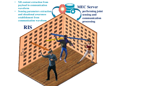
Figure 1: Illustrative example of the proposed THz system model for joint communication and sensing in XR applications.

Each RIS consists of a two-dimensional large antenna array that has an array of subarray (AoSA) structure as in [10]. In this structure, the antenna elements of the same subarray are connected to the same phase shifter and radio frequency (RF) chain, thus reducing the amount of phase shifters needed compared to a fully-connected array structure. Each subarray constitutes an RIS unit that has a square shape and a large number of antennas $M$. The antenna spacing within each RIS subarray is $\delta_{m}$. The total number of subarrays is $N$ with the spacing between subarrays being $\Delta_{N}$. These subarrays collectively adopt a hybrid beamforming architecture. Without loss of generality, we assume $N\geq U$, thus providing XR users with sufficient degrees of freedom in terms of association. This subarray structure allows us to have $N$ independent channels for a single RIS. The RISs are static and their locations are known a priori by other RISs. Let $\boldsymbol{v}^{b,n}=\left[v^{b,n}_{x},v^{b,n}_{y}\right]^{T}\in\mathbb{R}^{2}$ be the position of the $n$th subarray of RIS $b\in\mathcal{B}$. The XR users are mobile and may change their locations and orientations at any point in time. Let $\boldsymbol{p}^{u}=\left[p^{u}_{x},p^{u}_{y}\right]^{T}\in\mathbb{R}^{2}$ be the position of the user $u$.

II-A Joint Communication and Sensing Model

Consider an arbitrary RIS in $\mathcal{B}$ that captures the situational awareness and mapping information, and receives high data rate XR content as shown in Fig. 1. We assume that the RIS has performed synchronization and initial beam alignment according to existing techniques (e.g. [11]). To maintain high-resolution real-time user tracking of the users and a situational awareness of the indoor area, the RIS will continuously collect a sequence of $T$ snapshots of the received uplink communication signal. These snapshots enable the RISs to estimate and track the angle of arrival (AoA), angle of departure (AoD), and of users as well as the location of obstacles leading to non-line-of-sight (NLoS) communications. Since we use indoor RISs, then blockages mostly occur due to bodies of the users.
Each XR user has a uniform linear array (ULA) of $Q$ antennas and $R$ RF chains. Hence, if all XR users are active, $U$ data signaling beams are sent simultaneously to the RIS. To mitigate the high effect of schemes, a is used to maintain high energy efficiency at the UE. The far-field electromagnetic (EM) wave condition is assumed to be met. After beamforming, the transmitted signal by the UE at subcarrier $k$ is $\boldsymbol{s}_{k}(t)=\boldsymbol{F}_{\mathrm{R}}(t)\boldsymbol{F}_{k}(t)\boldsymbol{x}_{k}(t),\quad\forall k=1,\ldots,K$, where $\boldsymbol{x}_{k}(t)\in\mathbb{C}^{l\times 1}$ is the transmitted uplink communication signal, $\boldsymbol{F}_{k}\in\mathbb{C}^{R\times l}$ is the digital precoding matrix for subcarrier $k$, and $\boldsymbol{F}_{\mathrm{R}}(t)\in\mathbb{C}^{Q\times R}$ is the RF precoder for all subcarriers. After processing the communication waveform of subcarrier $k$, the uplink received signal at each RIS subarray $n$ will be:

$$y_{n,k}(t)=\boldsymbol{w}_{n,k}^{T}\boldsymbol{H}_{n,u}^{k}(t)\boldsymbol{s}_{k}(t)+\nu_{n,k}(t),$$ (1)

where $\boldsymbol{w}_{n,k}\in\mathbb{C}^{M\times 1}$ is the combining vector of RIS subarray $n$ at subcarrier $k$, $\boldsymbol{H}_{n,u}^{k}\in\mathbb{C}^{M\times Q}$ is the uplink channel matrix for subcarrier $k$, and $\nu_{n,k}\sim\mathcal{C}\mathcal{N}\left(\boldsymbol{0},\boldsymbol{I}_{M\times Q}\right)$ is the additive Gaussian noise vector at subarray $n$ and subcarrier $k$. To construct a single realization for sensing the wireless environment, $T$ snapshots are recorded by the RIS, each of which captures $J$ uplink measurements:

$$\boldsymbol{y}_{n,k}(t)=\boldsymbol{W}_{n,k}^{T}\boldsymbol{H}_{n,u}^{k}(t)\boldsymbol{F}_{\mathrm{R}}^{m}(t)\boldsymbol{F}_{k}(t)\boldsymbol{s_{k}}(t)+\boldsymbol{\nu}_{n,k}(t),$$ (2)

where $\boldsymbol{y}_{n,k}(t)\triangleq\left[y_{n,k,1}(t)\ldots y_{n,k,J}(t)\right]^{T},\boldsymbol{\nu}_{n,k}(t)\triangleq\left[\nu_{n,k,1}(t)\ldots\nu_{n,k,J}(t)\right]^{T},\boldsymbol{W_{n,k}}\triangleq\left[\boldsymbol{w}_{n,k,1}\ldots\boldsymbol{w}_{n,k,J}\right].$ Moreover, the $M\times Q$ MIMO channel matrix between user $u$ and RIS subarray $n$ in the time domain can be written as: $\boldsymbol{H}_{n,u}(t)=\sum_{p=1}^{P}\alpha^{p}_{n,u}\boldsymbol{a_{r}}\left(\phi^{p}_{n,u}\right)\boldsymbol{a_{t}}^{H}\left(\theta^{p}_{n,u}\right)\delta(t-\tau_{n,u}),$ where $\left(.\right)^{H}$ is the conjugate transpose, $\alpha^{l}_{n,u}\in\mathbb{C}$ is the complex channel gain, $P$ is the number of distinct spatial paths, $\theta_{n,u}^{l}$ is the AoD of the $p$th path of antenna $u$, $\tau_{n,u}$ is the of the path, $\phi_{n,u}^{p}$ is the AoA of the $p$th path at subarray $n$, and $\boldsymbol{a_{t}}\left(\theta^{p}_{n,u}\right)=\frac{1}{\sqrt{Q}}\left[1,e^{j\frac{2\pi}{\delta_{m}}\sin\left(\theta^{p}_{n,u}\right)},\cdots,e^{j(Q-1)\frac{2\pi}{\delta_{n}}\sin\left(\theta^{p}_{n,u}\right)}\right]^{T}$ is the array steering vector of the antenna array of the XR UE $\boldsymbol{a_{r}}\left(\phi^{pk}_{n,u}\right)=\frac{1}{\sqrt{M}}\left[1,e^{j\frac{2\pi}{\delta_{m}}\sin\left(\phi^{p}_{n,u}\right)},\cdots,e^{j(M-1)\frac{2\pi}{\delta_{n}}\sin\left(\phi^{p}_{n,u}\right)}\right]^{T}$ is the array steering vector of the RIS subarray that has a ULA structure Consequently, the channel matrix in the frequency domain associated with the $k$th subcarrier is given by:

$$\boldsymbol{H}^{k}_{n,u}(f)=\sum_{p=1}^{P}\alpha^{p}_{n,u}\boldsymbol{a_{r}}\left(\phi^{p}_{n,u}\right)\boldsymbol{a_{t}}^{H}\left(\theta^{p}_{n,u}\right)\exp\left(-\frac{j2\pi f\tau_{n,u}}{K}\right).$$ (3)

The snapshots in (2) can be collected over LoS or NLoS communication signal waveforms. In the case of a LoS uplink transmission, the channel gain will be [12]: $\alpha^{L}_{n,u}=\frac{c}{4\pi fr_{n,u}}e^{-\frac{k(f)r_{n,u}}{2}}e^{-j2\pi f\tau^{L}_{n,u}}.$ Here, $c$ is the speed of light, $k(f)$ is the overall molecular absorption coefficients of the medium at THz band, $f$ is the operating frequency, and $r_{n,u}$ is the distance between the XR user $u$ and the RIS subarray $n$. From this channel gain, we can see that in LoS conditions, the parameters to be estimated are $\{\theta^{L}_{n,u},\phi^{L}_{n,u},\tau^{L}_{n,u}\}$. This process allows tracking XR users in real-time. Here, we do not consider NLoS links for communications purposes due to the poor propagation characteristics of THz signals (e.g., limited reflection) and their high susceptibility to blockage. That is, such a NLoS link cannot meet the high-rate XR needs. Nonetheless, from a sensing standpoint, instead of discarding the NLoS signal completely, we use it to track the user and gather a situational awareness of the blockage incidence. In NLoS conditions, the channel gain is given by [13]:

$$\alpha^{N}_{n,u}=\frac{c}{4\pi f(r^{(1)}_{n,u}+r^{(2)}_{n,u})}e^{\left({-\frac{k(f)(r^{(1)}_{n,u}+r^{(2)}_{n,})}{2}}\right)}R(f)e^{-j2\pi f\tau^{N}_{n,u}},$$ (4)

where $r^{(1)}_{n,u}$ is the distance between the XR user $u$ and the reflecting point, and $r^{(2)}_{n,u}$ is the distance between the reflecting point and the RIS subarray $n$. For reflections, we consider the transverse electric part of the EM wave, that is, the signal is assumed to be perpendicular to the plane of incidence. This assumption is valid given the placement of our RIS as shown in Fig. 1. As such, $R_{n,u}(f)=\gamma_{n,u}(f)\rho_{n,u}(f)$ is the reflection coefficient, where $\gamma(f)\approx-\exp\left(\frac{-2\cos\left(\psi_{n,u}\right)}{\sqrt{\eta(f)^{2}-1}}\right)$ is the Fresnel reflection coefficient and $\rho_{n,u}(f)=\exp\left(-\frac{8\pi^{2}f^{2}\sigma^{2}\cos^{2}\left(\psi_{n,u}\right)}{c^{2}}\right)$ is the Rayleigh factor that characterizes the roughness effect. $\psi_{n,u}$ is the angle of the incident signal to the reflector, $\eta(f)$ is the refractive index, and $\sigma$ is the surface height standard deviation. Thus, for NLoS, the parameters to be estimated are: $\{\theta^{N}_{n,u},\phi^{N}_{n,u},\tau^{N}_{n,u},\psi_{n,u}\}$. Next, we formulate the problem of estimating the sensing parameters from the $J$ collected snapshots in (2). To do so, we leverage the sparsity of the THz channel matrix and reformulate the received uplink signal expression as a tensor.

III Situational Awareness Estimation via Tensor Decomposition

III-A Problem Formulation

Estimating the sensing parameters from $T$ communication snapshots recorded at the RIS subarray faces multiple challenges. First, existing estimation techniques [14, 15, 16] rely on the collection of pilot signals and their goal is to estimate the channel. In contrast, our goal here is to collect uplink communication signals that are being used by XR users during an XR session so as to continuously track the sensing parameters. Second, existing parameter estimation methods suffer from particular caveats: Off-grid methods like cannot jointly estimate multiple sensing parameters, leading to a difficult pairing problem [17]. Also, the algorithm cannot be readily applied to the peculiar AoSA structure of hybrid THz beamforming systems as the complexity of the method becomes impractical with large antenna arrays [18]. Moreover, on-grid methods like compressive sensing are constrained by their grid spacing, which increases complexity if a high-resolution is desired.
To successfully estimate the THz sensing parameters, we concatenate $T$ snapshots of the received uplink signal:

$$\boldsymbol{Y}_{n,k}=\boldsymbol{W}_{n,k}^{T}\boldsymbol{H}_{n,u}^{k}(f)\boldsymbol{\Omega}+\boldsymbol{N}_{n,k},$$ (5)

$$\boldsymbol{Y}_{n,k}\triangleq\left[\begin{array}[]{lll}\boldsymbol{y}_{n,k}(1)\ldots&\boldsymbol{y}_{n,k}(T)\end{array}\right],$$

$$\boldsymbol{N}_{n,k}\triangleq\left[\begin{array}[]{lll}\boldsymbol{\nu}_{n,k}(1)&\ldots&\boldsymbol{\nu}_{n,k}(T)\end{array}\right],$$

$$\boldsymbol{\Omega}\triangleq\left[\begin{array}[]{lll}\boldsymbol{F}_{\mathrm{R}}^{m}(1)\boldsymbol{F}_{k}(1)\boldsymbol{s_{k}}(1)&\ldots&\boldsymbol{F}_{\mathrm{R}}^{m}(T)\boldsymbol{F}_{k}(T)\boldsymbol{s_{k}}(T)\end{array}\right].$$

From (5), we observe that the received signal has three modes that represent the number of measurements, the number of snapshots, and the number of subcarriers, respectively. Thus, we can model it as a three-order tensor, namely, $\boldsymbol{\chi}\in\mathbb{C}^{J\times T\times K}$. In fact, substituting (3) in (5):

$$\boldsymbol{Y}_{n,k}(t) =\sum_{p=1}^{P}\Lambda_{n,u,k}^{p}\boldsymbol{\zeta}(\phi^{p}_{n,u})\boldsymbol{\xi}(\theta^{p}_{n,u})^{H}+\boldsymbol{N}_{n,k}.$$ (6)

In (6), $\Lambda_{n,u,k}^{p}\triangleq\alpha^{p}_{n,u}\exp(-\frac{j2\pi f\tau_{n,u}}{K})$, $\boldsymbol{\zeta_{k}}(\phi^{p}_{n,u})\triangleq\boldsymbol{W}_{n,k}^{T}\boldsymbol{a_{r}}\left(\phi^{p}_{n,u}\right)$, and $\boldsymbol{\xi_{k}}(\theta^{p}_{n,u})\triangleq\boldsymbol{\Omega}^{H}\boldsymbol{a_{t}}\left(\theta^{p}_{n,u}\right)$. Consequently, we can see that each slice $\boldsymbol{Y}_{n,k}$ corresponding to the tensor $\boldsymbol{\chi}$ is a weighted sum of a common set of rank-one outer products. Hence, we can factorize the tensor as follows:

$$\boldsymbol{\chi}=\sum_{p=1}^{P}\boldsymbol{\zeta_{k}}(\phi^{p}_{n,u})\circ\boldsymbol{\xi_{k}}(\theta^{p}_{n,u})\circ\Lambda_{n,u}^{p}+\mathcal{W}=\left[\left[\mathbf{A},\mathbf{B},\mathbf{C}\right]\right]+\mathcal{W},$$

$$\boldsymbol{A} \triangleq\left[\begin{array}[]{lll}\boldsymbol{\zeta}_{1}(\phi_{n,u}^{P})&\ldots&\boldsymbol{\zeta}_{K}(\phi_{n,u}^{P})\end{array}\right],$$ (7)

$$\boldsymbol{B} \triangleq\left[\begin{array}[]{lll}\boldsymbol{\xi}_{1}(\theta^{p}_{n,u})&\ldots\boldsymbol{\xi}_{K}(\theta^{p}_{n,u})&\end{array}\right],$$

$$\boldsymbol{C} \triangleq\left[\begin{array}[]{lll}\boldsymbol{\Lambda}_{n,u,1}^{p}&\ldots&\boldsymbol{\Lambda}_{n,u,K}^{p}\end{array}\right].$$

Here, $\circ$ is the outer product symbol, $\boldsymbol{\Lambda}_{n,u,k}^{p}=\left\{\alpha^{p}_{n,u}\exp(-\frac{j2\pi f\tau_{n,u}}{K})\right\}_{t=1}^{T}$, and $\mathcal{W}$ is $\boldsymbol{N}_{n,k}$ in the tensor domain. $\boldsymbol{A},\boldsymbol{B},$ and $\boldsymbol{C}$ are the three factor matrices associated to the tensor $\boldsymbol{\chi}$.

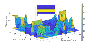
(a)

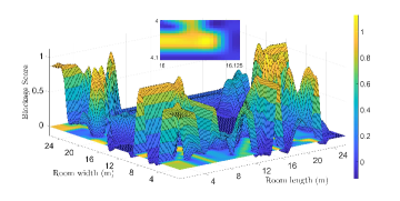
(b)

Figure 2: Spatial blockage score mapping at $f=$0.275\text{\,}\mathrm{T}\mathrm{H}\mathrm{z}$$ (a) $W=$7\text{\,}\mathrm{G}\mathrm{H}\mathrm{z}$$, (b) $W=$15\text{\,}\mathrm{G}\mathrm{H}\mathrm{z}$$, whereby a better resolution and more continuous visualizations are observed for higher bandwidths.

Here, we make some important remarks. First, owing to the THz channel’s sparsity and the few number of paths $P$, the tensor decomposition method becomes more efficient given that the uniqueness of this decomposition is guaranteed. Second, our approach can characterize the sensing parameters from the collected snapshots without imposing additional constraints or assumptions. For instance, alternatively adopting matrix factorization almost never leads to a unique solution unless the rank of the matrix is one or further conditions are imposed on the factor matrices.

III-B Proposed Sensing Parameters Estimation Method

After factorizing the tensor $\boldsymbol{\chi}$, extracting the sensing parameters and estimating them requires solving the following optimization problem:

$$\min_{\widetilde{\boldsymbol{A}},\widetilde{\boldsymbol{B}},\widetilde{\boldsymbol{C}}}\left\|\boldsymbol{\chi}-\sum_{p=1}^{P}\widetilde{\boldsymbol{a}}_{p}\circ\tilde{\boldsymbol{b}}_{p}\circ\widetilde{\boldsymbol{c}}_{p}\right\|_{F}^{2},$$ (8)

where $\widetilde{\mathbf{A}}=\left[\widetilde{\boldsymbol{a}_{1}}\cdots\widetilde{\boldsymbol{a}}_{P}\right],\widetilde{\boldsymbol{B}}=\left[\widetilde{\boldsymbol{b}}_{1}\cdots\widetilde{\boldsymbol{b}}_{P}\right],\widetilde{\boldsymbol{C}}=\left[\widetilde{\boldsymbol{c}}_{1}\cdots\widetilde{\boldsymbol{c}}_{P}\right]$ are the three estimated factor matrices. To solve this problem, the three factor matrices need to be estimated. To do so, we leverage the sparsity of the THz channel that guarantees the uniqueness condition for tensor decomposition. This allows us to establish a relationship between the true factor matrices and their estimates. Thus, given these relationships we derive the environmental sensing parameters as follows:

Proposition 1

The AoA, AoD, and corresponding to path $p$ between RIS subarray $n$ and user $u$ are:

$$\widetilde{\phi}^{P}_{n,u}=\arg\max_{\phi^{P}_{n,u}}\frac{\left|\widetilde{\boldsymbol{a}}_{k}^{H}\tilde{\boldsymbol{\zeta}}_{k}\left(\phi^{P}_{n,u}\right)\right|}{\left\|\widetilde{\boldsymbol{a}}_{k}\right\|_{2}\left\|\tilde{\boldsymbol{\zeta}}_{k}\left(\phi^{P}_{n,u}\right)\right\|_{2}},$$ (9)

$$\widetilde{\theta}^{P}_{n,u}=\arg\max_{\theta^{P}_{n,u}}\frac{\left|\widetilde{\boldsymbol{b}}_{k}^{H}\tilde{\boldsymbol{\xi}}_{k}\left(\theta^{P}_{n,u}\right)\right|}{\left\|\widetilde{\boldsymbol{b}}_{k}\right\|_{2}\left\|\tilde{\boldsymbol{\xi}}_{k}\left(\theta^{P}_{n,u}\right)\right\|_{2}},$$ (10)

$$\widetilde{\tau}^{P}_{n,u}=\arg\min_{\tau^{P}_{n,u}}\frac{\left|\widetilde{\boldsymbol{c}}_{k}^{H}\tilde{\boldsymbol{\Lambda}}^{P}_{n,u,k}\left(\theta^{P}_{n,u}\right)\right|}{\left\|\widetilde{\boldsymbol{c}}_{k}\right\|_{2}\left\|\tilde{\boldsymbol{\Lambda}}^{P}_{n,u,k}\left(\tau^{P}_{n,u}\right)\right\|_{2}}.$$ (11)

Proof:

See Appendix A ∎

(9)-(11) can be solved by performing a one-dimensional search. Thus, the estimated AoA, AoD, and allow us to track the XR user in near real-time (after collecting and processing the $T$ snapshots). Subsequently, after obtaining $\widetilde{\phi}^{P}_{n,u},\widetilde{\theta}^{P}_{n,u},$ and $\widetilde{\tau}^{P}_{n,u}$, the attenuation factor $\alpha^{P}_{n,u}$ can be obtained by substitution. Moreover, the proposed Algorithm 1 enables the RIS to track the users in real-time and characterize the spatial availability of communications.

Algorithm 1 High-resolution situational awareness mapping

while XR Session do

    Initialize real-time tracking mesh and blockage score mesh respectively: $\boldsymbol{E(t)}$ and $\boldsymbol{\Sigma(t)}.$

    if $\alpha^{P}_{n,u}\geq\epsilon$ then

        LoS link, determine $\boldsymbol{p}^{u}=\left[p^{u}_{x},p^{u}_{y}\right]^{T}$ from:

        $\phi_{n,u}^{L}=\arctan\frac{p^{u}_{y}-v^{b,n}_{y}}{p^{u}_{x}-v^{b,n}_{x}}$ and $\tau_{n,u}^{L}=\frac{\left\|\boldsymbol{p}^{u}-\boldsymbol{v}^{b,n}\right\|}{c}.$

    else if $\alpha^{P}_{n,u}\leq\epsilon$ then

        NLoS link:

        Determine $\psi_{n,u}$ from (4) while using the refractive $\eta$ index

        of human skin.

        Determine $r^{(1)}_{n,u}$ and $r^{(2)}_{n,u}$ by substituting $\phi_{n,u}^{N},\theta_{n,u}^{P},$ and $\psi_{n,u}$

        into the sine law equation.

        Determine obstacle location $\boldsymbol{o}^{n,u}=\left[o^{n,u}_{x},o^{n,u}_{y}\right]^{T}.$

        Determine $\boldsymbol{p}^{u}=\left[p^{u}_{x},p^{u}_{y}\right]$ from:

        $\phi_{n,u}^{L}=\arctan\frac{p^{u}_{y}-o^{n,u}_{y}}{p^{u}_{x}-o^{n,u}_{x}}.$

        $r^{(1)}_{n,u}=\sqrt{\left(p^{u}_{x}-o^{n,u}_{x}\right)^{2}+\left(p^{u}_{y}-o^{n,u}_{y}\right)^{2}}.$

    end if

    for $i=\boldsymbol{p}^{u}$ or $i=\boldsymbol{o}^{n,u}$ do

        $\boldsymbol{e}_{i}(t)\leftarrow 1.$

        $\boldsymbol{\sigma}_{i}(t)\leftarrow\boldsymbol{\sigma}_{i}(t-1)+1.$

    end for

    for $i=\boldsymbol{r}^{L}_{n,u}$ or $i=\boldsymbol{r}^{1}_{n,u}$ $i=\boldsymbol{r}^{2}_{n,u}$ do

        $\boldsymbol{\sigma}_{i}(t)\leftarrow\boldsymbol{\sigma}_{i}(t-1)+1.$

    end for

    Normalize blockage score map: $\bar{\boldsymbol{\Sigma}}(t)=\frac{\boldsymbol{\Sigma(t)}}{\arg\max_{\boldsymbol{\sigma}(t)}\boldsymbol{\Sigma}(t)}.$

end while

First, owing to the high gap between LoS and NLoS links, the channel gain estimated is compared to a threshold to distinguish LoS from NLoS links. Second, based on the LoS or NLoS operation, the position of the user and blocker (if available) are calculated from the estimated parameters, setup geometry, and the refractive index of human skin. Then, based on the obtained positions and orientations, a normalized spatial blockage map for every set of snapshots is evaluated. This map’s goal is to provide RISs with a near real-time estimate of the environment dynamics.
In our subsequent simulations, we obtain a realization of blockage score mapping while varying the system bandwidth to understand the system tradeoffs. We also compare the spectral efficiency and reliability of our system to frameworks without joint sensing and communications.

IV Simulation Results and Analysis

For our simulations, the RISs are deployed over the three walls of an indoor area modeled as a square of size $$24\text{\,}\mathrm{m}$\times$24\text{\,}\mathrm{m}$$. The molecular absorption was obtained from the sub-THz model in [19] with $1\%$ of water vapor molecules. For our parameters, we have: $N=$64\text{\,}$$ antennas, $Q=$32\text{\,}$$ antennas, $f=$0.275\text{\,}\mathrm{T}\mathrm{H}\mathrm{z}$$, $W=$10\text{\,}\mathrm{G}\mathrm{H}\mathrm{z}$$ (unless mentioned otherwise), and $p=$30\text{\,}\mathrm{d}\mathrm{B}\mathrm{m}$$. All statistical results are averaged over a large number of independent runs. The network was simulated with data generated from XR users moving according to a random walk which constitutes the most general scheme for user mobility.
Fig. 2 shows the effect of varying the bandwidth on the spatial blockage score map. That is, in the figure’s close-up we can see how a higher bandwidth visualizes a more continuous range of values for the blockage score. This is attributed to the fact that environmental sensing parameters extracted at a higher bandwidth can be computed at higher resolutions. It should be emphasized that increasing the bandwidth on the one hand, improves the data rate of our communication system, and on the other hand enhances our sensing resolution. Thus, our proposed approach does not face a rate-resolution tradeoff. On the contrary, these two metrics are positively correlated.
Fig. 3 shows the system reliability versus the number of users. Here, the system reliability follows the definition in [12], i.e., the probability that the E2E delay falls below a particular threshold. The E2E delay includes both downlink an uplink delays which include the processing, queuing, and transmission time (and beam tracking when valid). The threshold used for the total E2E delay here is $20\text{\,}\mathrm{m}\mathrm{s}$. We can see that our proposed approach has a higher reliability in static, low, and high mobility. Here, low mobility refers to a walking speed of XR users, i.e., $4.5\text{\,}\mathrm{k}\mathrm{m}\mathrm{/}\mathrm{h}$, and high mobility refers to a higher pace of $9\text{\,}\mathrm{k}\mathrm{m}\mathrm{/}\mathrm{h}$. Fig. 3 shows that the highest gains achieved using our proposed approach is in a low mobility setup, i.e., a $10\text{\,}\%$ improvement for the average number of users and a $19\text{\,}\%$ improvement for $U=20$, whereby the mapping configured captures the real-time state of the environment. Moreover, in a static setup, sensing information is not very useful. In contrast, for high mobility, the sensing measurements may lag the instantaneous dynamics and thus induce delays.
In Fig. 4, the total spectral efficiency defined as in [20] is shown. Fig. 4 clearly shows the benefits reaped from deploying a joint sensing and communication system that shares hardware, waveform, and spectrum. In fact, our proposed joint sensing and communication approach achieves a $42\text{\,}\%$ and $75\text{\,}\%$ improvement respectively compared to a communication system with beam training and a standalone sensing and communication system.

V Conclusion

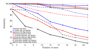
Figure 3: System reliability versus number of users

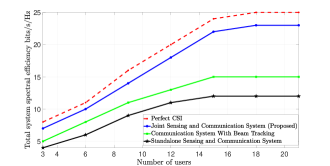
Figure 4: Spectral efficiency versus number of users

In this paper, we have proposed a new joint sensing and communication system framework for wireless XR at THz frequency bands. In particular, we have opportunistically used uplink communication waveforms for interleaved user and environment tracking. In particular, we have exploited the sparsity of THz channels to extract unique sensing parameters from the received uplink signals. Subsequently, a high-resolution indoor mapping is derived so as to characterize the spatial availability of communications and the blockage score of the area. Such a mapping allows us to reduce the need for a continuous beam tracking and improves the overall spectrum efficiency of the system.

-A Proof of Proposition 1

Problem (8) can be solved efficiently by the alternating least squares matrix factorization procedure [21]. Since we deal with a third order tensor, this factorization has three iterative steps. Then, it fixes two factor matrices and minimizes the error with respect to the considered factor matrix as:

$$\small\widetilde{\boldsymbol{A}}^{(t+1)}=\arg\min_{\widetilde{\boldsymbol{A}}}\left\|\boldsymbol{Y}_{n,(1)}^{T}-\left(\widetilde{\boldsymbol{C}}^{(t)}\odot\widetilde{\boldsymbol{B}}^{(t)}\right)\widetilde{\boldsymbol{A}}^{T}\right\|_{F}^{2},$$

$$\small\widetilde{\boldsymbol{B}}^{(t+1)}=\arg\min_{\widetilde{\boldsymbol{B}}}\left\|\boldsymbol{Y}_{n,(2)}^{T}-\left(\widetilde{\boldsymbol{C}}^{(t)}\odot\widetilde{\boldsymbol{A}}^{(t+1)}\right)\widetilde{\boldsymbol{B}}^{T}\right\|_{F}^{2},$$

$$\small\widetilde{\boldsymbol{C}}^{(t+1)}=\arg\min_{\widetilde{\boldsymbol{C}}}\left\|\boldsymbol{Y}_{n,(3)}^{T}-\left(\widetilde{\boldsymbol{B}}^{(t+1)}\odot\widetilde{\boldsymbol{A}}^{(t+1)}\right)\widetilde{\boldsymbol{C}}^{T}\right\|_{F}^{2},$$ (12)

where, $\odot$ is the Khatri-Rao product symbol. The exact factor matrices are related to their estimates according to: $\widetilde{\boldsymbol{A}}=\boldsymbol{A}\boldsymbol{\Upsilon}_{1}\boldsymbol{\Gamma}+\boldsymbol{E}_{1},\hskip 2.84544pt\widetilde{\boldsymbol{B}}=\boldsymbol{B}\boldsymbol{\Upsilon}_{2}\boldsymbol{\Gamma}+\boldsymbol{E}_{2},\hskip 2.84544pt\widetilde{\boldsymbol{C}}=\boldsymbol{C}\boldsymbol{\Upsilon}_{3}\boldsymbol{\Gamma}+\boldsymbol{E}_{3},$ where $\{\boldsymbol{\Upsilon_{1}},\boldsymbol{\Upsilon_{2}},\boldsymbol{\Upsilon_{3}}\}$ are unknown nonsingular diagonal matrices that satisfy $\boldsymbol{\Upsilon_{1}}\boldsymbol{\Upsilon_{2}}\boldsymbol{\Upsilon_{3}}=\boldsymbol{I}$, $\boldsymbol{\Gamma}$ is an unknown permutation matrix, and $\{\boldsymbol{E_{1}},\boldsymbol{E_{2}},\boldsymbol{E_{3}}\}$ are estimation error matrices. By applying a maximum likelihood estimator on each of the equations and assuming that the estimation error matrices $\{\boldsymbol{E_{1}},\boldsymbol{E_{2}},\boldsymbol{E_{3}}\}$ follow an independently and identically distributed (i.i.d.) circularly symmetric Gaussian distribution [22], we obtain (9), (10), and (11).

References

- [1] W. Saad, M. Bennis, and M. Chen, “A vision of 6G wireless systems: Applications, trends, technologies, and open research problems,” IEEE network, vol. 34, no. 3, pp. 134–142, Oct. 2020.
- [2] H. Sarieddeen, M.-S. Alouini, and T. Y. Al-Naffouri, “An overview of signal processing techniques for terahertz communications,” Proceedings of the IEEE, vol. 109, no. 10, pp. 1628–1665, Aug. 2021.
- [3] M. Ahmadipour, M. Kobayashi, M. Wigger, and G. Caire, “An information-theoretic approach to joint sensing and communication,” arXiv preprint arXiv:2107.14264, 2021.
- [4] Q. Zhang, X. Wang, Z. Li, and Z. Wei, “Design and performance evaluation of joint sensing and communication integrated system for 5g MmWave enabled CAVs,” IEEE Journal of Selected Topics in Signal Processing, Sept. 2021.
- [5] S. Buzzi, C. D’Andrea, and M. Lops, “Using massive MIMO arrays for joint communication and sensing,” in Proc. of the 53rd Asilomar Conference on Signals, Systems, and Computers, Pacific Grove, CA, USA, Nov. 2019, pp. 5–9.
- [6] A. M. Elbir, K. V. Mishra, and S. Chatzinotas, “Terahertz-band joint ultra-massive MIMO radar-communications: Model-based and model-free hybrid beamforming,” arXiv preprint arXiv:2103.00328, 2021.
- [7] A. Guerra, F. Guidi, D. Dardari, and P. M. Djurić, “Real-time learning for THz radar mapping and uav control,” in Proc. of IEEE International Conference on Autonomous Systems (ICAS), Montreal, QC, Canada, Aug 2021, pp. 1–5.
- [8] C. Chaccour, M. N. Soorki, W. Saad, M. Bennis, P. Popovski, and M. Debbah, “Seven defining features of terahertz (THz) wireless systems: A fellowship of communication and sensing,” arXiv preprint arXiv:2102.07668, 2021.
- [9] E. Basar, M. Di Renzo, J. de Rosny, M. Debbah, M.-S. Alouini, and R. Zhang, “Wireless communications through reconfigurable intelligent surfaces,” arXiv preprint arXiv:1906.09490, 2019.
- [10] A. Faisal, H. Sarieddeen, H. Dahrouj, T. Y. Al-Naffouri, and M.-S. Alouini, “Ultramassive MIMO systems at terahertz bands: Prospects and challenges,” IEEE Vehicular Technology Magazine, vol. 15, no. 4, pp. 33–42, Oct. 2020.
- [11] A.-A. A. Boulogeorgos and A. Alexiou, “Performance evaluation of the initial access procedure in wireless THz systems,” in Proc. of the 16th International Symposium on Wireless Communication Systems (ISWCS), Oulu, Finland, Aug. 2019, pp. 422–426.
- [12] C. Chaccour, M. N. Soorki, W. Saad, M. Bennis, and P. Popovski, “Can terahertz provide high-rate reliable low latency communications for wireless VR?” arXiv preprint arXiv:2005.00536, 2020.
- [13] A. Moldovan, M. A. Ruder, I. F. Akyildiz, and W. H. Gerstacker, “LOS and NLOS channel modeling for terahertz wireless communication with scattered rays,” in Proc. of IEEE Globecom Workshops (GC Wkshps), pp. 388–392.
- [14] R. Mendrzik, F. Meyer, G. Bauch, and M. Z. Win, “Enabling situational awareness in millimeter wave massive MIMO systems,” IEEE Journal of Selected Topics in Signal Processing, vol. 13, no. 5, pp. 1196–1211, Aug. 2019.
- [15] C. D. Ozkaptan, E. Ekici, O. Altintas, and C.-H. Wang, “OFDM pilot-based radar for joint vehicular communication and radar systems,” in Proc. of IEEE Vehicular Networking Conference (VNC), Taipei, Taiwan, Dec. 2018, pp. 1–8.
- [16] A. Guerra, F. Guidi, D. Dardari, and P. M. Djuric, “Near-field tracking with large antenna arrays: Fundamental limits and practical algorithms,” arXiv preprint arXiv:2102.05890, 2021.
- [17] M. H. Gruber, “Statistical digital signal processing and modeling,” 1997.
- [18] G. Zhu, K. Huang, V. K. Lau, B. Xia, X. Li, and S. Zhang, “Hybrid beamforming via the kronecker decomposition for the millimeter-wave massive MIMO systems,” IEEE Journal on Selected Areas in Communications, vol. 35, no. 9, pp. 2097–2114, Jun. 2017.
- [19] J. Kokkoniemi, J. Lehtomäki, and M. Juntti, “A line-of-sight channel model for the 100–450 gigahertz frequency band,” EURASIP Journal on Wireless Communications and Networking, vol. 2021, no. 1, pp. 1–15, Apr. 2021.
- [20] A. R. Chiriyath, B. Paul, and D. W. Bliss, “Radar-communications convergence: Coexistence, cooperation, and co-design,” IEEE Transactions on Cognitive Communications and Networking, vol. 3, no. 1, pp. 1–12, Feb. 2017.
- [21] N. D. Sidiropoulos, L. De Lathauwer, X. Fu, K. Huang, E. E. Papalexakis, and C. Faloutsos, “Tensor decomposition for signal processing and machine learning,” IEEE Transactions on Signal Processing, vol. 65, no. 13, pp. 3551–3582, Apr. 2017.
- [22] Z. Zhou, J. Fang, L. Yang, H. Li, Z. Chen, and R. S. Blum, “Low-rank tensor decomposition-aided channel estimation for millimeter wave mimo-ofdm systems,” IEEE Journal on Selected Areas in Communications, vol. 35, no. 7, pp. 1524–1538, Apr 2017.