Generalization Performance of Empirical Risk Minimization on Over-parameterized Deep ReLU Nets

Abstract

In this paper, we study the generalization performance of global minima for implementing empirical risk minimization (ERM) on over-parameterized deep ReLU nets. Using a novel deepening scheme for deep ReLU nets, we rigorously prove that there exist perfect global minima achieving almost optimal generalization error rates for numerous types of data under mild conditions. Since over-parameterization is crucial to guarantee that the global minima of ERM on deep ReLU nets can be realized by the widely used stochastic gradient descent (SGD) algorithm, our results indeed fill a gap between optimization and generalization of deep learning.

I Introduction

Deep learning [27] that conducts feature exaction and statistical modelling on a unified deep neural network (deep net) framework has attracted enormous research activities in the past decade. It has made significant breakthroughs in numerous applications including computer vision [32], speech recognition [33] and go games [57]. Simultaneously , it also brings several challenges in understanding the running mechanism and magic behind deep learning, among which the generalization issue in statistics [59] and convergence issue in optimization [2] are crucial.

The generalization issue pursues theoretical advantages of deep learning via presenting its better generalization capability than shallow learning such as kernel methods and shallow networks. Along with the rapid development of deep nets in approximation theory [16, 43, 58, 48, 55, 54, 18], essential progress on the excellent generalization performance of deep learning has been made in [29, 8, 37, 53, 17, 25]. To be detailed, [53] proved that implementing empirical risk minimization (ERM) on deep ReLU nets is better than shallow learning in embodying the composite structure of the well known regression function [24]; [25] showed that implementing ERM on deep ReLU nets succeeds in improving the learning performance of shallow learning by capturing the group-structure of inputs; and [17] derived that, with the help of massive data, implementing ERM on deep ReLU nets is capable of reflecting spatially sparse properties of the regression function while shallow learning fails. In a word, with appropriately selected number of free parameters, the generalization issue of deep learning seems to be successfully settled in terms that deep learning can achieve optimal learning rates for numerous types of data, which is beyond the capability of shallow learning.

The convergence issue concerns the convergence of some popular algorithms such as the stochastic gradient descent (SGD) and adaptive moment estimation (Adam) to solve ERM on deep nets. Due to the highly nonconvex nature, it is generally difficult to find global minima of such ERM problems, since there are numerous local minima, saddle points, plateau and even some flat regions [22]. It is thus highly desired to declare when and where the corresponding SGD or Adam converges. Unfortunately, in the under-parameterized setting exhibited in [29, 8, 37, 53, 17, 25], the convergence issue remains open. Alternatively, studies in optimization theory show that over-parameterizing deep ReLU nets enhance the convergence of SGD [21, 41, 2, 1]. In fact, it was proved in [2, 1] that SGD converges to either a global minimum or a local minimum near some global minimum of ERM, provided there are sufficiently many free parameters in deep ReLU nets. Noting further that implementing ERM on over-parameterized deep ReLU nets commonly yields infinitely many global minima and usually leads to over-fitting, it is difficult to verify the good generalization performance of the obtained global minima in theory.

As mentioned above, there is an inconsistency between generalization and convergence issues of deep learning in the sense that good generalization requires under-parameterization of deep ReLU nets while provable convergence needs over-parameterization, which makes the running mechanism of deep learning be still a mystery. Such an inconsistency stimulates to rethink the classical bias-variance trade-off in modern machine learning practice [12], since numerical evidences in [59] illustrated that there are over-parameterized deep nets generalizing well despite they achieved extremely small training error. In particular, [9] constructed an exact interpolation of training data that achieves optimal generalization error rates based on Nadaraya-Watson kernel estimates; [7] derived a sufficient condition for the data under which the global minimum of over-parameterized linear regression possesses excellent generalization performance; [36] studied the generalization performance of kernel-based least norm interpolation and presented generalization error estimates under some restrictions on the data distribution. Similar results can also be found in [11, 26, 45, 38, 6] and references therein. All these exciting results provide a springboard to understand benign over-fitting in modern machine-learning practice and present novel insights in developing learning algorithms to avoid the traditional bias-variance dilemma. However, it should be pointed out that these existing results are incapable of settling the generalization and convergence challenges of deep learning, mainly due to the following three aspects:

$\bullet$ Difference in model: the existing theoretical analysis for benign over-fitting is only available to convex linear models, but ERM on deep ReLU nets involves highly nonconvex nonlinear models.

$\bullet$ Difference in theory: the existing results for benign over-fitting focus on pursuing the restrictions on data distributions so that all global minima for over-parameterized linear models are good learners, which does not hold for deep learning, since it is easy to provide a counterexample for benign over-fitting of deep ReLU nets, even for noise-less data (see Proposition 1 below).

$\bullet$ Difference in requirements of dimension: Theoretical analysis in the existing work frequently requires the high dimensionality assumption of the input space, while the numerical experiments in [59] showed that deep learning can lead to benign over-fitting in both high and low dimensional input spaces.

Based on these three interesting observations, there naturally arises the following problem:

Problem 1

Without strict restrictions on data distributions and dimensions of input spaces, are there global minima of ERM on over-parameterized deep ReLU nets achieving the optimal generalization error rates obtained by under-parameterized deep ReLU nets?

There are roughly two schemes to settle the inconsistency between optimization and generalization for deep learning. One is to pursue the convergence guarantee for SGD on under-parameterized deep ReLU nets and the other is to study the generalization performance of implementing ERM on over-parameterized deep ReLU nets. To the best of our knowledge, there isn’t any theoretical analysis for the former, even when strict restrictions are imposed on the data distributions. An answer to Problem 1, a stepping-stone to demonstrate the feasibility of the latter, not only provides solid theoretical evidences for the benign over-fitting phenomenon of deep learning in practice [59], but also presents theoretical guidance on setting network structures to balance the generalization and optimization inconsistency.

The aim of the present paper is to present an affirmative answer to Problem 1. Our main tool for analysis is a novel network deepening approach based on the localized approximation property [16, 17] and product-gate property [58, 48] of deep nets. The network deepening approach succeeds in constructing over-parameterized deep nets (student network) via deepening and widening an arbitrary under-parameterized network (teacher network) so that the obtained student network exactly interpolates the training data and possesses almost the same generalization capability as the teacher network. In this way, setting the teacher network to be the one in [29, 8, 37, 53, 17, 25], we actually prove that there are global minima for ERM on over-parameterized deep ReLU nets that possess optimal generalization error rates, provided that the networks are deeper and wider than the corresponding student network.

The main contributions of the paper are two folds. Since the presence of noise is a crucial factor to result in over-fitting and it is not difficult to design learning algorithms with good generalization performance to produce perfect fit for noiseless data [34, 14], our first result is then to study the generalization capability of deep ReLU nets that exactly interpolate noiseless data. In particular, we construct a deep ReLU net that exactly interpolates the noiseless data but performs extremely badly in generalization and also prove that for deep ReLU nets with more than two hidden layers, there always exist global minima of ERM that can generalize extremely well, provided the number of free parameters achieves a certain level and the data are noiseless. This is different from the linear models studied in [9, 11, 12, 26, 36, 45, 38, 6] and shows the difficulty in analyzing over-parameterized deep ReLU nets. Our second result, more importantly, focuses on the existence of a perfect global minimum of ERM on over-parameterized deep ReLU nets that achieves almost optimal generalization error rates for numerous types of data. Using the network deepening approach, we rigorously prove that, if the depth and width of a deep net are larger than specific values, then there always exists such a perfect global minimum. This finding partly demonstrates the reason of the benign over-fitting phenomenon of deep learning and shows that implementing ERM on over-parameterized deep nets can derive an estimator of high quality. Different from the existing results, our analysis requires neither high dimensionality of the input space nor strong restrictions on the covariance matrix of the input data.

The rest of this paper is organized as follows. In the next section, after introducing the deep ReLU nets, we provide theoretical guarantee for the existence of good deep nets interpolant for noiseless data. In Section III, we present our main results via rigorously proving the existence of perfect global minima. In Section IV, we compare our results with related work and present some discussions. In Section V, we conduct numerical experiments to verify our theoretical assertions. We prove our results in the last section.

II Global Minima of ERM on Over-Parameterized Deep Nets for Noiseless Data

Let $L\in\mathbb{N}$ be the depth of a deep net, $d_{0}=0$ and $d_{\ell}\in\mathbb{N}$ be the width of the $\ell$-th hidden layer for $\ell=1,\dots,L-1$. Denote by the affine operator $\mathcal{J}_{\ell}:\mathbb{R}^{d_{\ell-1}}\rightarrow\mathbb{R}^{d_{\ell}}$ with $\mathcal{J}_{\ell}(x):=W_{\ell}x+b_{\ell}$ for $d_{\ell}\times d_{\ell-1}$ weight matrix $W_{\ell}$ and bias vector $b_{\ell}\in\mathbb{R}^{d_{\ell}}$. For the ReLU function $\sigma(t)=t_{+}:=\max\{t,0\}$, write $\sigma(x)=(\sigma(x^{(1)}),\dots,\sigma(x^{(d)}))^{T}$ for $x=(x^{(1)},\dots,x^{(d)})^{T}$. Define an $L$-layer deep ReLU net by

$$\mathcal{N}_{d_{1},\dots,d_{L}}(x)=a\cdot\sigma\circ\mathcal{J}_{L}\circ\sigma\circ\mathcal{J}_{L-1}\circ\dots\circ\sigma\circ\mathcal{J}_{1}(x),$$ (1)

where $a\in\mathbb{R}^{d_{L}}$. The structure of $\mathcal{N}_{d_{1},\dots,d_{L}}$ is determined by the weight matrices $W_{\ell}$ and bias vectors $b_{\ell}$, $\ell=1,\dots,L$. In particular, full weight matrices correspond to deep fully connected nets (DFCN) [58]; sparse weight matrices are associated with deep sparsely connected nets (DSCN) [48]; and Toeplitz-type weight matrices are related to deep convolutional neural networks (DCNN) [60]. In particular, for DFCN, we have the number of training parameters

$$n=d_{L}+\sum_{\ell=1}^{L}(d_{\ell-1}d_{\ell}+d_{\ell})$$ (2)

and for DSCN, $n$ is much smaller than the number in (2). In this paper, we mainly focus on analyzing the benign over-fitting phenomenon for DFCN. Denote by $\mathcal{N}_{d_{1},\dots,d_{L}}^{DFCN}$ the set of all DFCNs of the form (1). Define the width of DFCN to be $U:=\max\{d,d_{1},\dots,d_{L}\}.$

Given a sample set $D=\{(x_{i},y_{i})_{i=1}^{m}\}$, we are interested in global minima of the following empirical risk minimization (ERM):

$${\arg\min}_{f\in\mathcal{N}_{d_{1},\dots,d_{L}}^{DFCN}}\frac{1}{m}\sum_{i=1}^{m}(f(x_{i})-y_{i})^{2}.$$ (3)

Denote by $\Psi_{{d_{1},\dots,d_{L}},m}$ the set of global minima of the optimization problem (3), i.e.,

$$\Psi_{d_{1},\dots,d_{L},m}:=\{f:f\ \mbox{is the solution to}\ (\ref{target-optimization})\}.$$ (4)

Before studying the quality of the global minima of (3), we present some properties of $\Psi_{d_{1},\dots,d_{L},m}$ in the following lemma.

Lemma 1

If $d_{1}\geq m$, then for any $L\geq 1$ and $d_{2},\dots,d_{L}\geq 2$, there are infinitely many functions in $\Psi_{d_{1},\dots,d_{L},m}$ and for any $f\in\Psi_{d_{1},\dots,d_{L},m}$, there holds $f(x_{i})=y_{i},i=1,\dots,m$.

Lemma 1 is a direct extension of [49, Theorem 5.1], where similar conclusion is drawn for $\mathcal{N}_{d_{1}}^{DFCN}$ with $d_{1}\geq m$. Based on [49, Theorem 5.1], the proof of Lemma 1 is obvious by noting $t=\sigma(t)-\sigma(-t)$ and $d_{2},\dots,d_{L}\geq 2$. Lemma 1 implies that if $m$ is sufficiently large and the network structure satisfying $d_{1}\geq m$, then there are always infinitely many solutions to (3) and any global minimum $f$ exactly interpolates the given data. It should be mentioned that similar results also hold for any DSCNs that contain a shallow net with $m$ neurons. Since we place particular emphasis on DFCN, we leave the corresponding assertions for DSCN for interested readers.

Let $\mathbb{I}^{d}:=[-1,1]^{d}$. Denote by $L^{p}(\mathbb{I}^{d})$ the space of $p$th-Lebesgue integrable functions endowed with norm $\|\cdot\|_{L^{p}(\mathbb{I}^{d})}$. In this section, we are concerned with noiseless data, that is, there is some $f^{*}\in L^{p}(\mathbb{I}^{d})$ such that

$$f^{*}(x_{i})=y_{i},\qquad i=1,\dots,m.$$ (5)

At first, we provide a negative result for running ERM on over-parameterized deep ReLU nets, showing that there is some $f\in\Psi_{{d_{1},\dots,d_{L}},m}$ performs extremely badly in generalization.

Proposition 1

Let $1\leq p<\infty$. If $L\geq 2$, $d_{1}\geq 4dm$, $d_{2}\geq m$ and $d_{3},\dots,d_{L}\geq 2$, then there are infinitely many $f\in\Psi_{d_{1},d_{2},\dots,d_{L},m}$ such that for any $f^{*}$ satisfying (5) and $\|f^{*}\|_{L^{p}(\mathbb{I}^{d})}\geq c$ there holds

$$\|f^{*}-f\|_{L^{p}(\mathbb{I}^{d})}\geq c/2,$$ (6)

where $c$ is an absolute constant.

Proposition 1 shows that in the over-parameterized setting, there are infinitely many global minima of (3) behaving extremely badly, even for the noiseless data. It should be highlighted that the construction of $f$ in our proof is independent of $f^{*}$. In fact, due to the localized approximation of deep ReLU nets, we can construct deep ReLU nets $f$ which can exactly interpolate the training sample but satisfy $\|f\|_{L^{p}(\mathbb{I}^{d})}\leq\varepsilon$ for arbitrarily small $\varepsilon>0$. Different from the results in [12, 26, 45, 36], it is difficult to quantify conditions on distributions and dimensions of input spaces such that all global minima of over-parameterized deep ReLU nets possess good generalization performances. This is mainly due to the nonlinear nature of the hypothesis space, though the capacities, measured by the covering numbers [23, 5], for deep ReLU nets and linear models are comparable, provided there are similar numbers of free parameters involved in hypothesis spaces and the depth is not so large.

Proposition 1 provides extremely bad examples for global minima of (3) in generalization, even for noiseless data. It seems that over-parameterized deep ReLU nets are always worse than under-parameterized networks, which is standard from a viewpoint of classical learning theory [19]. However, in our following theorem, we will show that if the number of free parameters increases to a certain extent, then there are also infinitely many global minima of (3) possessing excellent generalization performance. To this end, we need two concepts concerning the data distribution and the smoothness of the target function $f^{*}$.

Denote $\Lambda:=\{x_{i}\}_{i=1}^{m}$ as the input set. The separation radius [46] of $\Lambda$ is defined by

$$q_{\Lambda}=\frac{1}{2}\min_{i\neq j}\|x_{i}-x_{j}\|_{2},$$ (7)

where $\|x\|_{2}$ denotes the Euclidean norm of $x\in\mathbb{R}^{d}$. The separation radius is half of the smallest distance between any two distinct points in $\Lambda$ and naturally satisfies $q_{\Lambda}\leq m^{-1/d}$. Let us also introduce the standard smoothness assumption [24, 58, 48, 37, 62]. Let $c_{0}>0$ and $r=s+\mu$ with $s\in\mathbb{N}_{0}:=\{0\}\cup\mathbb{N}$ and $0<\mu\leq 1$. We say a function $f:\mathcal{A}\subseteq\mathbb{R}^{d}\rightarrow\mathbb{R}$ is $(r,c_{0})$-smooth if $f$ is $s$-times differentiable and for every $\alpha_{j}\in\mathbb{N}_{0}$, $j=1,\dots,d$ with $\alpha_{1}+\dots+\alpha_{d}=s$, its $s$-th partial derivative satisfies the Lipschitz condition

$$\left|\frac{\partial^{s}f}{\partial x_{1}^{\alpha_{1}}\dots\partial x_{d}^{\alpha_{d}}}(x)-\frac{\partial^{s}f}{\partial x_{1}^{\alpha_{1}}\dots\partial x_{d}^{\alpha_{d}}}(x^{\prime})\right|\leq c_{0}\|x-x^{\prime}\|_{2}^{\mu},\quad\forall\ x,x^{\prime}\in\mathcal{A}.$$ (8)

Denote by $Lip_{\mathcal{A}}^{(r,c_{0})}$ the set of all $(r,c_{0})$-smooth functions defined on $\mathcal{A}$.

We are in a position to state our first main result to show the existence of good global minima of (3) for noiseless data.

Theorem 2

Let $r,c_{0}>0$ and $N\in\mathbb{N}$. If $f^{*}\in Lip_{\mathbb{I}^{d}}^{(r,c_{0})}$ satisfies (5), $N\succeq q_{\Lambda}^{-d}$, $L\succeq\log N$, $d_{1}\succeq N$ and $d_{\ell}\succeq\log N$ for $\ell=2,\dots,L$, then there are infinitely many $h^{*}\in\Psi_{d_{1},\dots,d_{L},m}$, such that

$$\|h^{*}-f^{*}\|_{L^{\infty}(\mathbb{I}^{d})}\leq CN^{-r/d},$$ (9)

where $C>0$ is a constant depending only on $r,d$ and $c_{0}$, and $a\succeq b$ for $a,b>0$ means that there is some constant $C^{\prime}$ depending only on $r,d$ and $c_{0}$ such that $a\geq C^{\prime}b$.

A consensus on deep nets approximation is that it can break the “curse of dimensionality”, which was verified in interesting work [43, 30, 55, 31, 18, 53] in terms of deriving dimension-independent approximation rates. However, it should be pointed out that to achieve such dimension-independent approximation rates, strict restrictions have been imposed on target functions, which become stronger as the dimension $d$ grows, just as [4, P.68] observed. In this way, though the approximation error of deep nets is independent of the dimension, the applicable target functions become more and more stringent as $d$ grows. Our result presented in Theorem 2 drives a different direction to show that even for well-studied smooth functions, there is a deep net that interpolates the training data without degrading the approximation rate. We highlight that the approximation rate depends on the a-priori knowledge of the target functions. In particular, if we impose strict restriction such as $f^{*}\in Lip_{\mathbb{I}^{d}}^{(r,c_{0})}$ with $r\geq d/2$, which is standard in kernel learning [15], then the approximation rate can be at least of order $n^{-1/2}$, which is also dimension-independent.

It is well known that deep learning has achieved great success in applications whose input space are of high dimensionality such as image processing [32] and game theory [57], showing the excellent performance of deep learning with large $d$. However, recent progress in inventory management [52], finance prediction [28] and earthquake intensity analysis [25] demonstrated that deep learning is also efficient for applications with low-dimensional input spaces. Therefore, numerous research activities have been triggered to verify the advantage of deep nets from approximation theory [58, 48, 61] and learning theory [29, 31, 17] that regarded $d$ as a constant. This paper follows from this direction to assume $d$ to be a constant and is much smaller than the size of data. As we mentioned above, if $d$ is extremely large, more restrictions on the target functions should be imposed, just as Theorem 4 below purports to show.

Noting that there are totally $\mathcal{O}(N\log N)$ parameters in $h^{*}$ in (9), the derived error rate is almost optimal in the sense that up to a logarithmic factor, the derived upper bound is of the same order of lower bound [58, 23], i.e., $C_{1}^{\prime}(N\log N)^{-r/d}$ for some $C_{1}^{\prime}>0$ independent of $N$. This means that for $N\succeq q_{\Lambda}^{-d}$ and $L\succeq\log N$, we can get almost optimal deep nets via finding suitable global minima of (3). Theorem 2 also shows that in the over-parameterized setting, where all global minima exactly interpolate the data, the interpolation restriction does not always affect the approximation performance of deep nets. Theorem 2 actually presents a sufficient condition for the number of free parameters of deep ReLU nets , $N\succeq q_{\Lambda}^{-d}$, to guarantee the existence of perfect global minima when we are faced with noiseless data. It should be highlighted that $q_{\Lambda}$ can be numerically determined, provided the data set is given. If $\{x_{i}\}_{i=1}^{m}$ are drawn identically and independently (i.i.d.) according to some distribution, the lower bound of $q_{\Lambda}$ is easy to be derived in theory [24, 36, 38].

III Global Minima of ERM on Over-Parameterized Deep Nets for Noisy Data

In this section, we conduct our study in the standard least-square regression framework [24, 19] and assume

$$y_{i}=f^{*}(x_{i})+\varepsilon_{i},\qquad i=1,\dots,m,$$ (10)

where $\{x_{i}\}_{i=1}^{m}$ are i.i.d. drawn according to an unknown distribution $\rho_{X}$ on an input space $\mathcal{X}\subseteq[0,1]^{d}$ and $\{\varepsilon_{i}\}_{i=1}^{m}$ are independent random variables that are independent of $\{x_{i}\}_{i=1}^{m}$ and satisfy $|\varepsilon_{i}|\leq 1$, $\mathbf{E}[\varepsilon_{i}]=0$, $i=1,\dots,m.$ Denote by $\Xi$ a set of Borel probability measures on $\mathcal{X}$ and $\Theta$ a set of functions defined on $\mathcal{X}$, respectively. Write

$$\mathcal{M}(\Theta,\Xi):=\{(\rho_{X},f^{*}):\rho_{X}\in\Xi,f^{*}\in\Theta\}.$$

Let $\Gamma_{D}$ be the class of all functions that are derived based on the data set $D$. Define

$$e(\Theta,\Xi):=\sup_{{(\rho_{X},f^{*})}\in\mathcal{M}(\Theta,\Xi)}\inf_{f_{D}\in\Gamma_{D}}\mathbf{E}(\|f^{*}-f_{D}\|^{2}_{L^{2}_{\rho_{X}}}).$$ (11)

It is easy to see that $e(\Theta,\Xi)$ measures the theoretically optimal generalization bound a learning scheme, based on data set $D$ satisfying (10), can achieve when $f^{*}\in\Theta$ and $\rho_{X}\in\Xi$ [24]. Our purpose is to compare generalization errors of the global minima defined by (3) with $e(\Theta,\Xi)$ to illustrate whether the global minima can achieve the theoretically optimal generalization error bounds.

Before presenting our main results, we introduce a negative result derived in [31, Theorem 2], which shows that without any restriction imposed to the distribution $\rho_{X}$, over-parameterized deep nets do not generalize well.

Lemma 2

If $d_{1}\geq m$, then for any $L\geq 1$ and $d_{2},\dots,d_{L}\geq 2$ and any $h\in\Psi_{d_{1},\dots,d_{L},m}$, there exists a probability measure $\rho_{X}^{*}$ on $\mathcal{X}$ such that

$$\sup_{f^{*}\in Lip_{\mathbb{I}^{d}}^{(r,c_{0})},\rho_{X}=\rho_{X}^{*}}\mathbf{E}[\|f^{*}-h\|^{2}_{L^{2}_{\rho_{X}^{*}}}]\geq 1/6.$$ (12)

Lemma 2 shows that without any restrictions to the distribution, even for the widely studied smooth functions, all of the global minima of (3) in the over-parameterized setting are bad estimators. This is totally different from the under-parameterized setting, in which distribution-free optimal generalization error rates were established [24, 40]. Lemma 2 seems to contradict with the numerical results in [59] at the first glance. However, we highlight that $\rho_{X}^{*}$ in (12) is a very special distribution that is even not continuous with respect to the Lebesgue measure. If we impose some mild conditions to exclude such distributions, then the result will be totally different.

The restriction we study in this paper is the following well known distortion assumption of $\rho_{X}$ [56, 17], which is slightly stricter than the standard assumption that $\rho_{X}$ is absolutely continuous with respect to the Lebesgue measure. Let $p\geq 2$ and $J_{p}$ be the identity mapping

$$L^{p}(\mathcal{X})~{}~{}{\stackrel{{\scriptstyle J_{p}}}{{\longrightarrow}}}~{}~{}L^{2}_{\rho_{X}}.$$

Define $D_{\rho_{X},p}:=\|J_{p}\|,$ where $\|\cdot\|$ denotes the operator norm. Then $D_{\rho_{X},p}$ is called the distortion of $\rho_{X}$ (with respect to the Lebesgue measure), which measures how much $\rho_{X}$ distorts the Lebesgue measure. In our analysis, we assume $D_{\rho_{X},p}<\infty$, which holds for the uniform distribution for all $p\geq 2$ obviously. Denote by $\Xi_{p}$ the set of $\rho_{X}$ satisfying $D_{\rho_{X},p}<\infty$.

We then provide optimal generalization error rates for global minima of (3) for different a-priori information. Let us begin with the widely used class of smooth regression functions. The classical results in [24] showed that

$$C_{1}m^{-\frac{2r}{2r+d}}\leq e(Lip^{(r,c_{0})}_{\mathbb{I}^{d}},\Xi_{p})\leq C_{2}{m}^{-\frac{2r}{2r+d}},\qquad p\geq 2,$$ (13)

where $C_{1}$, $C_{2}$ are constants independent of $m$ and $e(Lip^{(r,c_{0})}_{\mathbb{I}^{d}},\Xi_{p})$ is defined by (11). It demonstrates the optimal generalization error rates for $f^{*}\in Lip^{(r,c_{0})}_{\mathbb{I}^{d}}$ and $\rho_{X}\in\Xi_{p}$ that a good learning algorithm should achieve. Furthermore, it can be found in [53, 25] that there is some network structure $\Phi_{n,L}$ such that all global minima of ERM on under-parameterized deep ReLU nets can reach almost optimal error rates in the sense that if $L\sim\log m$, $d_{1}\sim m^{\frac{d}{2r+d}}$ and $d_{2},\dots,d_{L}\sim\log m$, then

$$C_{1}m^{-\frac{2r}{2r+d}}\leq\sup_{f^{*}\in Lip^{(r,c_{0})}_{\mathbb{I}^{d}},\rho_{X}\in\Xi_{p}}\mathbf{E}[\|f^{under}_{global}-f^{*}\|_{L_{\rho_{X}^{2}}}^{2}]\leq C_{3}\left(\frac{m}{\log m}\right)^{-\frac{2r}{2r+d}},$$ (14)

where $C_{3}$ is a constant depending only on $r,c_{0},d,p$ and $f^{under}_{global}$ is an arbitrary global minimum of (3) with depth and width specified as above.

It follows from (14) and (13) that all global minima of ERM on under-parameterized deep ReLU nets are almost optimal learners to tackle data i.i.d. drawn according to $\rho\in\mathcal{M}(Lip^{(r,c_{0})},\Xi_{p})$. In the following theorem, we show that, if the network is deepened and widened, there also exist global minima of (3) for over-parameterized deep ReLU nets possessing similar generalization performance.

Theorem 3

Let $p\geq 2$, $r,c_{0}>0$. If $L\succeq\log m$, $d_{1}\succeq m$ and $d_{2},\dots,d_{L}\succeq\log m$, then there exist infinitely many $h\in\Psi_{d_{1},\dots,d_{L},m}$ such that

$$C_{1}m^{-\frac{2r}{2r+d}}\leq\sup_{f^{*}\in Lip^{(r,c_{0})}_{\mathbb{I}^{d}},\rho_{X}\in\Xi_{p}}\mathbf{E}[\|h-f^{*}\|_{L_{\rho_{X}}^{2}}^{2}]\leq 2C_{3}\left(\frac{m}{\log m}\right)^{-\frac{2r}{2r+d}}.$$ (15)

Due to Lemma 1, any $h\in\Psi_{d_{1},\dots,d_{L},m}$ is an exact interpolant of $D$, i.e. $h(x_{i})=y_{i}$, $i=1,\dots,m$. Therefore, Theorem 3 presents theoretical verifications of benign over-fitting for deep ReLU nets, which was intensively discussed recently [9, 12, 36, 38, 7]. It should be mentioned that our main novelties are two folds. On one hand, we are concerned with deep ReLU nets while the existing results focused on linear hypothesis spaces. On the other hand, we provide evidence of existence of good global minima without high-dimensionality and strong distribution assumptions while the existing results focused on searching strong conditions on the dimension of input spaces and data distributions to guarantee that all global minima have excellent generalization performances.

Theorem 3 shows that implementing ERM on over-parameterized deep ReLU nets can achieve the almost optimal generalization error rates, but it does not demonstrate the power of depth since shallow learning also reaches these bounds [15, 40]. To show the power of depth, we should impose more restrictions on regression functions. For this purpose, we introduce the generalized additive models that are widely used in statistics and machine learning [24, 53]. For $r,\gamma,c_{0},c_{0}^{\prime}>0$, we say that $f$ admits a generalized additive model if $f=h\left(\sum_{i=1}^{d}f_{i}(x^{(i)})\right),$ where $h\in Lip^{(r,c_{0})}_{\mathbb{R}}$ and $f_{i}\in Lip^{(\gamma,c_{0}^{\prime})}_{\mathbb{I}}$. Write $\mathcal{W}_{r,\gamma,c_{0},c_{0}^{\prime}}$ as the set of all functions admitting a generalized additive model. If $L\sim\log m$, $d_{1}\sim m^{\frac{1}{2r+1}}$ and $d_{2},\dots,d_{L}\sim\log m$, it can be found in [53, 25] that for any $p\geq 2$, there holds

$$C_{4}\left(m^{-\frac{2r}{2r+1}}+m^{-\frac{2\gamma(r\wedge 1)}{2\gamma(r\wedge 1)+1}}\right)\leq e(\mathcal{W}_{r,\gamma,c_{0},c_{0}^{\prime}},\Xi_{p})$$ (16)

$$\leq \sup_{f^{*}\in\mathcal{W}_{r,\gamma,c_{0},c_{0}^{\prime}},\rho_{X}\in\Xi_{p}}\mathbf{E}[\|f_{global}^{under}-f^{*}\|_{L^{2}_{\rho_{X}}}^{2}]$$

$$\leq C_{5}\left(m^{-\frac{2r}{2r+1}}+m^{-\frac{2\gamma(r\wedge 1)}{2\gamma(r\wedge 1)+1}}\right)\log^{3}m,$$

where $C_{4}$, $C_{5}$ are constants independent of $m$ and $f_{global}^{under}$ is an arbitrary global minimum of (3). Noticing that shallow learning is difficult to achieve the above generalization error rates: even for a special case of the generalized additive model with $f_{i}(x^{(i)})=(x^{(i)})^{2}$, it has been proved in [18] that shallow nets with any activation functions cannot achieve the aforementioned generalization error rates. The following theorem presents the existence of perfect global minima of (3) to show the power of depth in the over-parameterized setting.

Theorem 4

Let $p\geq 2$ and $r,\gamma,c_{0},c_{0}^{\prime}>0$. If $L\succeq\log m$, $d_{1}\succeq m$, and $d_{2},\dots,d_{L}\succeq\log m$, then there are infinitely many $h\in\Psi_{d_{1},\dots,d_{L},m}$ such that

$$C_{4}\left(m^{-\frac{2r}{2r+1}}+m^{-\frac{2\gamma(r\wedge 1)}{2\gamma(r\wedge 1)+1}}\right)\leq\sup_{f^{*}\in\mathcal{W}_{r,\gamma,c_{0},c_{0}^{\prime}},\rho_{X}\in\Xi_{p}}\mathbf{E}[\|h-f^{*}\|_{L_{\rho_{X}}^{2}}^{2}]$$ (17)

$$\leq 2C_{5}\left(m^{-\frac{2r}{2r+1}}+m^{-\frac{2\gamma(r\wedge 1)}{2\gamma(r\wedge 1)+1}}\right)\log^{3}m.$$

Theorem 4 shows that there are infinitely many global minima of ERM on over-parameterized deep ReLU nets theoretically breakthroughing the bottleneck of shallow learning. This illustrates an advantage of adopting over-parameterized deep ReLU nets to build up hypothesis spaces in practice.

Finally, we show the power of depth in capturing the widely used spatially sparse features with the help of massive data. It has been discussed in [17, 39] that spatial sparseness is an important data feature for image and signal processing and deep ReLU nets perform excellently in reflecting the spatial sparseness. Partition $\mathbb{I}^{d}$ by $(N^{*})^{d}$ sub-cubes $\{A_{j}\}_{j=1}^{(N^{*})^{d}}$ of side length $(N^{*}){-1}$ and with centers $\{\zeta_{j}\}_{j=1}^{(N^{*})^{d}}$. For $u\in\mathbb{N}$ with $u\leq(N^{*})^{d}$, define

$$\Upsilon_{u}:=\left\{j_{\ell}:j_{\ell}\in\{1,2,\dots,(N^{*})^{d}\},1\leq\ell\leq u\right\}.$$

If the support of $f\in L^{p}(\mathbb{I}^{d})$ is contained in $S:=\cup_{j\in\Upsilon_{u}}A_{j}$ for a subset $\Upsilon_{u}$ of $\{1,2,\dots,(N^{*})^{d}\}$ of cardinality at most $u$, we then say that $f$ is $u$-sparse in $(N^{*})^{d}$ partitions. Denote by $Lip^{(N^{*},u,r,c_{0})}_{\mathbb{I}^{d}}$ the set of all $f\in Lip^{(r,c_{0})}_{\mathbb{I}^{d}}$ which are $s$-sparse in $(N^{*})^{d}$ partitions. Let $L\sim\log m$, $d_{1},d_{2}\sim\left(m\left(\frac{u}{(N^{*})^{d}}\right)/\log m\right)^{1/(2r+d)}$, $d_{3},\dots,d_{L}\sim\log m$. If $m$ is large enough to satisfy $\frac{m}{\log m}\geq\tilde{C}_{4}\frac{(N^{*})^{\frac{2d+4r+2d}{(2r+d)p}}}{u^{\frac{1}{2r+d}}},$ then it can be easily deduced from [17] that there exists a DSCN structure contained in $\mathcal{N}_{d_{1},\dots,d_{L}}^{DFCN}$ such that

$$C_{6}m^{-\frac{2r}{2r+d}}\left(\frac{u}{(N^{*})^{d}}\right)^{\frac{d}{2r+d}}\leq e(Lip^{(N^{*},u,r,c_{0})}_{\mathbb{I}^{d}},\Xi_{p})$$ (18)

$$\leq \sup_{\rho\in\mathcal{M}(Lip^{((N^{*})^{d},u,r,c_{0})},\Xi_{p})}\mathbf{E}[\|f_{global}^{under}-f^{*}\|_{L^{2}_{\rho_{X}}}^{2}]$$

$$\leq C_{7}\left(\frac{m}{\log m}\right)^{-\frac{2r}{2r+d}}\left(\frac{u}{(N^{*})^{d}}\right)^{\frac{2}{p}-\frac{2r}{2r+d}},$$

where $\tilde{C}_{4},C_{6},C_{7}$ are constants independent of $m$ and $f_{global}^{under}$ is an arbitrary global minimum of ERM on the DSCN. In (18), $\left(\frac{m}{\log m}\right)^{-\frac{2r}{2r+d}}$ reflects the smoothness of $f^{*}$ and $\left(\frac{u}{(N^{*})^{d}}\right)^{\frac{2}{p}-\frac{2r}{2r+d}}$ embodies the spatial sparseness of $f^{*}$. As discussed above, given a sparsity level $u$ and the number of partitions $(N^{*})^{d}$, the size of data should satisfy $\frac{m}{\log m}\geq\tilde{C}_{4}\frac{(N^{*})^{\frac{2d+4r+2d}{(2r+d)p}}}{u^{\frac{1}{2r+d}}}$ to embody the spatially sparse feature of $f^{*}$. In particular, if the number of samples is smaller than the sparsity level $u$, it is impossible to develop learning schemes to realize the support of $f^{*}$. Recalling the localized approximation property of deep ReLU nets [16, 17], with the help of massive data, (18) shows that deep ReLU nets are capable of capturing the spatial sparseness, which is beyond the capability of shallow nets due to its lack of localized approximation [16]. We refer the readers to [17] for more details about the above assertions. If $p=2$, it can be found in (18) that ERM on deep ReLU nets in the under-parameterized setting can achieve almost optimal generalization error rates. The following theorem shows the existence of perfect global minima of (3) in the over-parameterized setting.

Theorem 5

Let $r,c_{0}>0$, $N^{*}\in\mathbb{N}$, $u\leq(N^{*})^{d}$ and $m$ satisfy $\frac{m}{\log m}\succeq\frac{(N^{*})^{\frac{2d+4r+2d}{(2r+d)p}}}{u^{\frac{1}{2r+d}}}.$ If $L\succeq\log m$, $d_{1},d_{2}\succeq m$ and $d_{3},\dots,d_{L}\succeq\log m$, then there are are infinitely many $h\in\Psi_{d_{1},\dots,d_{L}}$ such that

$$C_{6}m^{-\frac{2r}{2r+d}}\left(\frac{u}{(N^{*})^{d}}\right)^{\frac{d}{2r+d}}\leq\sup_{\rho\in\mathcal{M}(Lip^{(N^{*},u,r,c_{0})},\Xi_{2})}\mathbf{E}[\|h-f^{*}\|_{L^{2}_{\rho_{X}}}^{2}]$$ (19)

$$\leq 2C_{7}\left(\frac{m}{\log m}\right)^{-\frac{2r}{2r+d}}\left(\frac{u}{(N^{*})^{d}}\right)^{\frac{d}{2r+d}}.$$ (20)

Theorem 5 shows that for spatially sparse regression functions, there are infinitely many global minima of (3) in the over-parameterized setting achieving the almost optimal generalization error rates. Besides the given three types of regression functions, we can provide similar results for numerous regression functions including the general composite functions [53], hierarchical interaction models [30] and piecewise smooth functions [29] by using the same approach in this paper. In particular, to derive similar assertions as our theorems, it is sufficient to apply the proposed deepening scheme developed in Theorem 6 below on the corresponding generalization error estimates in [30, 29, 53]. We remove the details for the sake of brevity.

Based on the above theorems, we can derive the following corollary, which shows the versatility of over-parameterized deep ReLU nets in regression.

Corollary 1

Let $p\geq 2$ and $r,\gamma,c_{0},c_{0}^{\prime}>0$, $N\in\mathbb{N}$, $u\leq N^{d}$ and $m$ satisfy $\frac{m}{\log m}\succeq\frac{N^{\frac{2d+4r+2d}{(2r+d)p}}}{u^{\frac{1}{2r+d}}}.$ If $L\succeq\log m$, $d_{1},d_{2}\succeq m$ and $d_{3},\dots,d_{L}\succeq\log m$, then there are are infinitely many $h\in\Psi_{d_{1},\dots,d_{L}}$ such that (14), (17), and (19) hold simultaneously.

A crucial problem of deep learning is on how to specify the structure of deep nets for a given learning task. It should be highlighted that in the under-parameterized setting, both the width and depth should be carefully tailored to avoid the bias-variance trade-off phenomenon, making the structures of deep nets for different learning tasks quite different [30, 29, 53, 17, 25]. However, as shown in Corollary 1, over-parameterizing succeeds in avoiding the structure selection problem of deep learning in the sense that there exist a unified over-parameterized structure of DFCN which contains perfect global minima for different learning tasks.

IV Related Work and Discussions

In this section, we review some related work on the generalization performance of deep ReLU nets and make some comparisons to highlight our novelty. From the classical bias-variance trade-off principle, the over-parameterized setting makes the deep nets model so flexible that its global minima suffer from the well known over-fitting phenomenon [19] in the sense that they fit the training data perfectly but fail to predict new query points. Surprisingly, numerical evidences [59] showed that the over-fitting may not occur. This interesting phenomenon leads to a rethinking of the modern machine-learning practice and bias-variance trade-off.

The interesting result in [9] is the first work, to the best of our knowledge, to theoretically study the generalization performance of interpolation methods. In [9], multivariate triangulations are constructed to interpolate data and the generalization error bounds are exhibited as a function with respect to the dimension $d$, which shows that the interpolation method possesses good generalization performance when $d$ is large. After imposing certain structure constraints on the covariance matrices, [26, 7] derived tight generalization error bounds for over-parameterized liner regression. In [45], the authors revealed several quantitative relations between linear interpolants and the structures of covariance matrices and then provided a hybrid interpolating scheme whose generalization error was rate-optimal for sparse liner model with noise. Motivated by these results, [36] proved that kernel ridgeless least squares possess a good generalization performance for high dimensional data, provided the distribution $\rho_{X}$ satisfies certain restrictions. In [38], the generalization error of kernel ridgeless least squares was proved to be bounded by means of some differences of kernel-based integral operators.

It should be mentioned that there are some strict restrictions concerning the dimensionality, structures of covariance matrices and marginal distributions $\rho_{X}$ to guarantee the good generalization performance of interpolation methods in the existing literature. Indeed, it was proved in [31] that some restriction on the marginal distribution $\rho_{X}$ is necessary, without which there is a $\rho_{X}^{*}$ such that all interpolation methods may perform extremely badly (see Lemma 2). However, the high dimensional assumption and structure constrains of covariance matrices are removable, since [9] have already constructed a piecewise interpolation based on the well known Nadaraya-Watson estimator and derived optimal generalization error rates, without any restrictions on the dimension and covariance matrices.

Compared with the above mentioned existing work, there are mainly three novelties of our results. First, we aim to explain the over-fitting resistance phenomenon for deep learning rather than linear algorithms such as linear regression and kernel regression. Due to the nonlinear nature of (3), we rigorously prove the existence of bad minima and perfect global ones. Therefore, it is almost impossible to derive the same results as linear models [12, 45, 36] for deep ReLU nets to determine which conditions are sufficient to guarantee the perfect generalization performance of all global minima. Furthermore, our theoretical results coincide with the experimental phenomenon in the sense that global minima (with training error to be 0) with different parameters frequently have totally different behaviors in generalization. Then, our results present essential advantages of running ERM on over-parameterized deep ReLU nets by means of proving the existence of deep ReLU nets possessing the almost optimal generalization error rates, which is beyond the capability of shallow learning. Finally, our results are established with mild conditions on distributions and without any restrictions on the dimension of the input space.

Another related work is [44], where the authors discussed the generalization performance of interpolation methods based on histograms and also established the existence of bad and good interpolation neural networks. The main arguments of [44] and our paper are similar: there are global minima of ERM on deep ReLU nets that can avoid over-fitting. The main differences are as follows: 1) It is well known that an approximant or learner based on histograms suffers from the well known saturation problem in the sense that the approximation or learning rate cannot be improved further once the regularity (or smoothness) of the regression function achieves certain level [58]. In particular, as shown in [58, 17], deep ReLU nets with two hidden layers can provide localized approximation but is difficult to approximate extremely smooth functions. In our paper, we avoid this saturation phenomenon via deepening the networks and thus break through the bottleneck of the analysis in [44]. 2) We provide detailed structures of deep ReLU nets and derive the quantitative requirement of the number of free parameters to guarantee the existence of global minima of ERM on deep ReLU nets, which is different from [44]. 3) More importantly, we devote to answering Problem 1 via showing the optimal generalization error rates and the power of depth of some global minima of ERM on deep ReLU networks. In particular, using the deepening approach, we prove that there exist infinitely many global minima of ERM on over-parameterized deep ReLU nets that perform almost the same as the under-parameterized deep ReLU nets.

In summary, we provide an affirmative answer to Problem 1 via providing several examples for perfect global minima of (3). It would be interesting to study the distribution of these perfect global minima and design feasible schemes to find them. We will keep in studying this topic and consider these two more challenging problems.

V Numerical Examples

In this section, we conduct numerical simulations to support our theoretical assertions on the existence of benign overfitting of running ERM on over-parameterized deep ReLU nets. There are mainly four purposes of our simulations. In the first simulation, we aim to show the relation between the generalization performance of global minima of (3) and the number of parameters (or width) of deep ReLU nets. In the second one, we devote to verifying the over-fitting resistance of (3) via showing the relation between the generalization error and the number of algorithmic iterations (epoches). In the third one, we show the existence of good and bad global minima of (3). Finally, we compare our learned global minima with some widely used learning schemes to show the learning performance of (3) on over-parameterized deep ReLU nets.

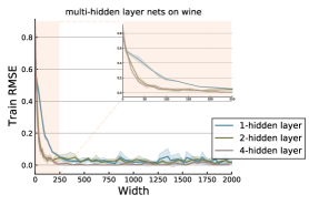
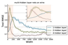
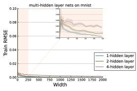
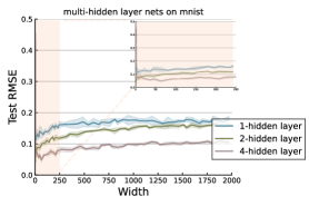
Figure 1: Relation between training and testing errors and the width

For these purposes, we adopt fully connected ReLU neural networks with $L$ hidden layers and $k$ neurons paved on each layer. In all simulations, we set $L\in\{1,2,4\}$ and $k\in\{1,\dots,2000\}.$ We use the well known Adam optimization algorithm on deep ReLU nets with step-size being constantly $0.001$ and initialization being the default PyTorch values. Without especial declaration, the training is stopped after $50,000$ iterations.

we report our results on two real-world data numerical simulations on two datasets. The first one is a Wine Quality dataset from UCI database. The Wine Quality dataset is related to red and white variants of the Portuguese “Vinho Verde” wine with $1599$ red and $4898$ white examples. We select white wine for experiments. There are $12$ attributes in the data set: fixed acidity, volatile acidity, citric acid, residual sugar, chlorides, free sulfur dioxide, total sulfur dioxide, density, pH, aulphates, alcohol and quality (score between $0$ and $10$). Therefore, it can be viewed as a regression task on input data of $11$ dimension. Regarding the preferences, each sample was evaluated by a minimum of three sensory assessors (using blind tastes), which graded the wine in a scale ranging from $0$ (very bad) to $10$ (excellent). We sample $2/3$ data points as our training set and $1/3$ for testing.

The second dataset is MNIST. MNIST dataset is widely used in classification tasks. Here we follow [36] to create a regression task using MNIST. MNIST inlcudes 70000 samples in total. Each sample includes a 28*28 dimensional feature and a target representing a digit ranging from 0 to 9. We randomly pick 291 samples with targeting digits equaling to 0 or 1, and separate 221 samples for training and 70 for testing. We label digit 0 as -1 and digit 1 as 1. Then we get a dataset with a $28\times 28=784$ dimensional feature and a label -1 or 1. The regression task is then built.

Simulation 1. In this simulation, we study the relation between the RMSE (rooted mean squared error) of test error and widths of deep ReLU nets with $L=1,2,4$. Our results are recorded via 5 independent single trials. The solid line is the mean value from these trials, and the shaded part indicates the deviation. The numerical results are reported in Figure 1.

Figure 1 presents the perfect global minima by exhibiting the relation between training and testing RMSE and the number of free parameters. From Figure 1, we obtain the following four observations: 1) The left figure shows that neural networks with more hidden layers are easier to produce exact interpolations of the training data. This coincides with the common consensus since more hidden layers with the same width involves much more free parameters; 2) For each depth, it can be found in the right figure that the testing curves exhibit an approximate doubling descent phenomenon as declared in [12] for linear models. It should be highlighted that such a phenomenon does not always exist for deep ReLU nets training and we only choose a good trend from several trails to demonstrate the existence of perfect global minima; 3) As the width (or capacity of the hypothesis space) increases, it can be found in the right figure that the testing error does not increase, exhibiting a totally different phenomenon from the classical bias-variance trade-off. This shows that for over-parameterized deep ReLU nets, there exist good global minima of (3), provided the depth is appropriately selected; 4) It can be found that deeper ReLU nets perform better in generalization, which demonstrates the power of depth in tackling the Wine Quality data. All these verify our theoretical assertions in Section III and show that there exist perfect global minima of (3) to realize the power of deep ReLU nets.

Simulation 2. In this simulation, we devote to numerically studying the role of iterations (epoches) in (3) in both under-parameterized and over-parameterized settings. We run ERM on DFCNs with depth 4 and width $2,40,2000$ on Wine dataset and MNIST dataset. Since the number of training data is 3265(221 in MNIST dataset, resp.), it is easy to check that deep ReLU nets with depth 4 and widths 2 and 40 are under-parameterized, while those with depth 4 and width 2000 is over-parameterized. The numerical results are reported in Figure 2.

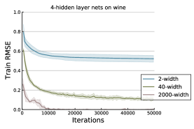
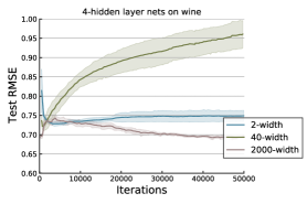
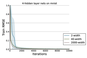
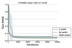
Figure 2: Relation between the training and testing errors and the number of iterations

There are also three interesting findings exhibited in Figure 3: 1) For under-parameterized ReLU nets, it is almost impossible to produce a global minimum acting as an exact interpolation of the data. However, for over-parameterized deep ReLU nets, running Adam with sufficiently many epoches attains a training error to be zero. Furthermore, after a specific value, the number of iterations does not affect the training error. This means that Adam converges to a global minimum of (3) on over-parameterized deep ReLU nets; 2) The testing error for under-parameterized ReLU nets, exhibited in the right figure, behaves according to the classical bias-variance trade-off principle in the sense that the error firstly decreases with respect to the epoch and then increases after a specific value of epoches. Therefore, early-stopping is necessary to guarantee the good performance in this setting; 3) The testing error for over-parameterized ReLU nets is always non-increasing with respect to the epoch. This shows the over-fitting resistance of deep ReLU nets training and also verifies the existence of the perfect global minima of (3) on over-parameterized deep ReLU nets. It should be highlighted the numerical result presented in Figure 3 is also a single trial selected from numerous results, since we are concerned with the existence of perfect global minima. In fact, there are also numerous examples for bad global minima of (3).

Simulation 3 In this simulation, we show that although there exist perfect global minima in over-parameterized settings, bad global minima can also be found sometimes. We test the performance of deep ReLU nets with depth 4 and width 2000 on Wine dataset and MNIST dataset. It take different numbers of steps to converge to a good training performance on these two datasets. We trigger several runs with different learning rates and net parameter initializations, and pick good and bad global minima from two trials respectively. We report the numerical results in Figure3.

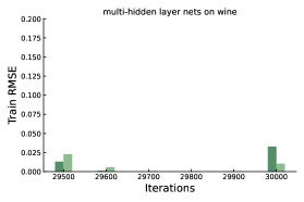
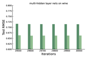
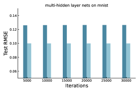
Figure 3: Comparison of good and bad global minima

From Figure 3, we find that different global minima of Figure 3 perform totally differently in generalization, though the training loss both comes to 0. In particular, the testing errors of bad global minima can be much larger than those of good global minima. It should be mentioned that the bad interpolants in the above simulations are also derived from Adam. Therefore, their orders of testing errors are comparable with those of good interpolants. We highlight that this is due to the implementation of the ADAM algorithm rather than the model (3). As far as the model is concerned, it can be shown in our next simulation that the orders of bad interpolants are also larger than those of good ones.

Simulation 4 In this simulation, we compare (3) on over-parameterized deep ReLU nets with some standard learning algorithms including ridge regression (Ridge), support vector regression (SVR), kernel interpolation(KIR) and kernel ridge regression (KRR) to show that the numerical phenomenon exhibited in previous figures is not built upon sacrificing the generalization performance. For the sake of fairness, we test various models under the same condition to our best efforts via tuning hyper-parameters. In particular, we implement the referenced methods by using the standard scikit-learn package. In the experiment with the wine dataset specifically, we use ridge regression with regularization parameter being $1$. In KRR, we use the Gaussian kernel with width being $20$ and regularization parameter being $0.0002$. KIR uses the Gaussian kernel with width being $5$ and regularization parameter being 0. SVR keeps the default sklearn hyper-parameters. In the experiment with the MNIST dataset, we change regularization parameter in ridge regression to 10 and keep other parameters fixed. In this simulation, we also use the deep ReLU nets with depth $4$ and width $2000$ and conduct 5 trials to record the average training and testing RMSE.

In addition, we construct a ReLU net that achieves 0 training error but performs extremely badly in the testing set to show that there really exist extremely bad interpolants, just as Proposition 1 illustrated. We introduce some notations at first. Denote $x_{i}=\left(x_{i}^{(1)},\ldots,x_{i}^{(d)}\right)$. Define $T_{\tau,a,b}(t)=\frac{1}{\tau}\{\sigma(t-a+\tau)-\sigma(t-a)-\sigma(t-b)+\sigma(t-b-\tau)\}$, where $\sigma$ is the ReLU activation function and $\tau$ is a parameter which we set to be small enough ($e^{-10}$ in this simulation). A feature input is expressed as $x=\left(x^{(1)},\ldots,x^{(d)}\right)$. We call the corresponding output of the constructed net (CN) as $N_{1,m,\tau}(x)$. Note that we drop duplicated samples when implementing CN. CN is constructed as bellow:

$$N_{1,m,\tau}(x)=\sum_{i=1}^{m}y_{i}\sigma\left(\sum_{l=1}^{d}T_{\tau,x_{i}^{(l)}-\frac{1}{m^{5}},x_{i}^{(l)}+\frac{1}{m^{5}}}\left(x^{(l)}\right)-(d-1)\right).$$

More details of the construction of $N_{1,m,\tau}$ can be found in the proof of Proposition 1. We introduce $N_{1,m,\tau}$ in this simulation is to show that as an interpolant, $N_{1}$ performs quite poorly to show that there are extremely bad global minima of (3). The numerical results are reported in Table I.

Wine Quality Data
	Methods	Train RMSE	Test RMSE
	Ridge	0.534	0.735
	kernel interpolation	0.000	13.031
	KRR	0.668	0.706
	SVR	0.628	0.696
	4-hidden layer DFCN (good case)	0.000	0.668
	CN (bad case)	0.000	5.931

MNIST Data
	Methods	Train RMSE	Test RMSE
	Ridge	0.056	0.304
	kernel interpolation	0.000	0.135
	KRR	0.031	0.140
	SVR	0.073	0.154
	4-hidden layer DFCN (good case)	0.000	0.097
	CN (bad case)	0.000	1.000

TABLE I: Comparison with other regression methods

There are four interesting observation in Table I: 1) Learning schemes such as SVR, KRR and Ridge perform stablely, since for both high-dimensional applications and low-dimensional simulations. The main reason is that a regularization term is introduced to balance the bias and variance for these schemes. As a result, the training error of these schemes are always non-zero; 2) Kernel interpolation performs well in high dimensional applications but fails to generalize well in low dimensional simulations. The main reason is that if $d$ is large, then the separation radius $q_{\Lambda}$ is large [36, 38], which in turn implies that the condition number of the kernel matrix is relatively small, making the kernel interpolation perform well. However, if $d$ is small, the condition number of the kernel matrix is usually extremely large, making the prediction instable; 3) There exist deep ReLU nets exactly interpolating the training data, leading to zero training error, but possessing an excellent generalization capability in yield small testing error, implying that the obtain estimator is a benign over-fitter for the data. Furthermore, it is shown in the table that the testing error of over-parameterized deep ReLU nets is the smallest, demonstrating the power of depth as declared in our theoretical assertions in Section III; 4) There also exist deep ReLU nets interpolating the data but performing extremely badly in generalization, for both high-dimensional applications and low dimensional simulations. All these findings verify our theoretical assertions that there are good global minima for ERM on over-parameterized deep ReLU nets but not all global minima are good.

VI Proofs

In this section, we aim at proving our results stated in Section II and Section III. The main novelty of our proof is a deepening scheme that produces an over-parameterized deep ReLU net (student network) based on a specific under-parameterized one (teacher network) so that the student network exactly interpolates the training data and possesses almost the same generalization performance as the teacher network.

VI-A Deepening scheme for ReLU nets

Given a teacher network $g$, the deepening scheme devotes to deepening and widening it to produce a student network $f$ that exactly interpolates the given data $D$ and possesses almost the same generalization performance as $g$. The following theorem presents the deepening scheme in our analysis.

Theorem 6

Let $g_{n,L,U}$ be any deep ReLU nets with $L$ layers, $n$ free parameters and width not larger than $U\in\mathbb{N}$ satisfying $\|g_{n,L,U}\|_{L^{\infty}(\mathbb{I}^{d})}\leq C^{*}$ for some $C^{*}>0$. If $\rho_{X}\in\Xi_{p}$ with $p\in[2,\infty)$, then for any $\varepsilon>0$, there exist infinitely many DFCNs $f_{D,n,L,U,g}$ of depth $\mathcal{O}(L+\log\varepsilon^{-1})$ and width $\mathcal{O}(m+U+\log\varepsilon^{-1})$ such that

$$f_{D,n,L,U,g}(x_{i})=y_{i},\qquad\ \forall i=1,\dots,m,$$ (21)

and

$$\|f_{D,n,L,U,g}-g_{n,L}\|_{L_{\rho_{X}}^{2}}\leq\varepsilon,$$ (22)

where $\tilde{C}$ is a constant depending only on $d$.

The deepening scheme developed in Theorem 6 implies that all deep ReLU nets that have been verified to possess good generalization performances in the under-parameterized setting [29, 53, 38, 25] can be deepened to corresponding deep ReLU nets in the over-parameterized setting such that the deepened networks exactly interpolate the given data and possess good generalization error bounds.

The main tools for the proof of Theorem 6 are the localized approximation property of deep ReLU nets developed in [17] and the product gate property of deep ReLU nets proved in [58]. Let us introduce the first tool as follows. For $a,b\in\mathbb{R}$ with $a<b$, define a trapezoid-shaped function $T_{\tau,a,b}$ with a parameter $0<\tau\leq 1$ as

$$T_{\tau,a,b}(t) := \frac{1}{\tau}\big{\{}\sigma(t-a+\tau)-\sigma(t-a)$$ (23)

$$- \sigma(t-b)+\sigma(t-b-\tau)\big{\}}.$$

We consider

$${\mathcal{N}}_{a,b,\tau}(x):=\sigma\left(\sum_{j=1}^{d}T_{\tau,a,b}(x^{(j)})-(d-1)\right).$$ (24)

The following lemma proved in [17] presents the localized approximation property of ${\mathcal{N}}_{a,b,\tau}$.

Lemma 3

Let $a<b$, $0<\tau\leq 1$ and ${\mathcal{N}}_{a,b,\tau}$ be defined by (24). Then we have $0\leq{\mathcal{N}}_{a,b,\tau}(x)\leq 1$ for all $x\in\mathbb{I}^{d}$ and

$${\mathcal{N}}_{a,b,\tau}(x)=\left\{\begin{array}[]{cc}0,&\mbox{if}\ x\notin[a-\tau,b+\tau]^{d},\\ 1,&\mbox{if}\ x\in[a,b]^{d}.\end{array}\right.$$ (25)

The second tool, as shown in the following lemma, presents the product-gate property of deep ReLU nets [58].

Lemma 4

For any $\ell\in\{2,3,\dots,\}$ and $\nu\in(0,1)$, there exists a DFCN with ReLU activation functions $\tilde{\times}_{\ell,\nu}:\mathbb{R}^{\ell}\rightarrow\mathbb{R}$ with $\mathcal{O}\left(\ell\log\frac{1}{\varepsilon}\right)$ depth, $\mathcal{O}\left(\ell\log\frac{1}{\varepsilon}\right)$ width, and free parameters bounded by $\mathcal{O}(\ell^{\beta}\nu^{-\beta})$ for some $\beta>0$ such that

$$|u_{1}u_{2}\cdots u_{\ell}-\tilde{\times}_{\ell,\nu}(u_{1},\dots,u_{\ell})|\leq\nu,\qquad\forall u_{1},\dots,u_{\ell}\in[-1,1]$$

and

$$\tilde{\times}_{\ell,\nu}(u_{1},\dots,u_{\ell})=0,\qquad\mbox{if}\quad u_{j}=0\quad\mbox{for some}\quad j=1,\dots,\ell.$$

With the above tools, we can prove Theorem 6 as follows.

Proof:

Let ${\mathcal{N}}_{\tau}={\mathcal{N}}_{-\tau,\tau,\tau/2}$ be given in Lemma 3 and $\tilde{\times}_{2,\nu}:\mathbb{R}^{2}\rightarrow\mathbb{R}$ in Lemma 4 with $\ell=2$. Then it follows from (25) that

$${\mathcal{N}}_{\tau}(x-x_{i})=\left\{\begin{array}[]{cc}0,&\mbox{if}\ x\notin x_{i}+[-3\tau/2,3\tau/2]^{d},\\ 1,&\mbox{if}\ x\in x_{i}+[-\tau,\tau]^{d}.\end{array}\right.$$ (26)

Since $\|g_{n,L,U}\|_{L^{\infty}(\mathbb{I}^{d})}\leq C^{*}$, we can define a function $\mathcal{N}_{\tau,\nu,D,g}$ on $\mathbb{R}^{d}$ by

$$\mathcal{N}_{\tau,\nu,D,g}(x) := \sum_{i=1}^{m}y_{i}{\mathcal{N}}_{\tau}(x-x_{i})$$ (27)

$$+ C^{*}\tilde{\times}_{2,\nu}\left(\frac{g_{n,L,U}(x)}{C^{*}},1-\sum_{i=1}^{m}{\mathcal{N}}_{\tau}(x-x_{i})\right).$$

If $\tau<\frac{2q_{\Lambda}}{3\sqrt{d}}$, then for any $j\neq i$, we have from (26) that ${\mathcal{N}}_{\tau}(x_{j}-x_{i})=0.$ Noting further ${\mathcal{N}}_{\tau}(x_{i}-x_{i})=1$, we have for any $j=\{1,\dots,m\}$ that $\sum_{i=1}^{m}{\mathcal{N}}_{\tau}(x_{j}-x_{i})=1$ and

$$\mathcal{N}_{\tau,\nu,D,g}(x_{j})=\sum_{i=1}^{m}y_{i}{\mathcal{N}}_{\tau}(x_{j}-x_{i})=y_{j}.$$ (28)

Moreover, for $i\neq j$ and any $x\in\mathbb{R}^{d}$,

$$\|x_{i}-x-(x_{j}-x)\|_{2}=\|x_{i}-x_{j}\|_{2}\geq\frac{2q_{\Lambda}}{\sqrt{d}}>3\tau$$

implies $\mathcal{N}_{\tau}(x-x_{j})=0.$ Hence $1-\sum_{i=1}^{m}\mathcal{N}_{\tau}(x-x_{i})\in[0,1]$. Therefore, Lemma 4 yields $\tilde{\times}_{2,\nu}\left(\frac{g_{n,L,U}(x_{j})}{C^{*}},1-\sum_{i=1}^{m}{\mathcal{N}}_{\tau}(x_{j}-x_{i})\right)=0$. This implies

$$\mathcal{N}_{\tau,\nu,D,g}(x_{j})=y_{j},\qquad j=1,\dots,m.$$ (29)

Define further a function $h_{D}$ on $\mathbb{R}^{d}$ by

$$h_{D}(x):=\sum_{i=1}^{m}y_{i}{\mathcal{N}}_{\tau}(x-x_{i})+g_{n,L,U}(x)\left(1-\sum_{i=1}^{m}{\mathcal{N}}_{\tau}(x-x_{i})\right).$$

It follows from Lemma 4 that

$$|h_{D}(x)-\mathcal{N}_{\tau,\nu,D,g}(x)|\leq\nu,\qquad\ \forall x\in\mathbb{I}^{d}.$$ (30)

If $x-x_{i}\notin[-3\tau/2,3\tau/2]^{d}$ for all $i=1,\dots,m$, then it follows from (26) that $\sum_{i=1}^{m}{\mathcal{N}}_{\tau}(x-x_{i})=0$, which implies $h_{D}(x)=g_{n,L}(x)$. Hence,

$$\|g_{n,L,U}-h_{D}\|_{L^{p}(\mathbb{I}^{d})}^{p}=\int_{\mathbb{I}^{d}}|g_{n,L,U}(x)-h_{D}(x)|^{p}dx$$

$$\leq \sum_{i=1}^{m}\int_{[x_{i}-3\tau/2,x_{i}+3\tau/2]^{d}}|g_{n,L,U}(x)-h_{D}(x)|^{p}dx\leq m(3\tau)^{d}2^{p}(C^{*})^{p}.$$

This implies

$$\|g_{n,L,U}-h_{D}\|_{L^{p}(\mathbb{I}^{d})}\leq 2C^{*}3^{d/p}m^{1/p}\tau^{d/p}.$$

The above estimate together with (30) yields

$$\|h_{D}-\mathcal{N}_{\tau,\nu,D,g}\|_{L^{p}(\mathbb{I}^{d})}\leq\|h_{D}-\mathcal{N}_{\tau,\nu,D,g}\|_{L^{p}(\mathbb{I}^{d})}+\|g_{n,L,U}-h_{D}\|_{L^{p}(\mathbb{I}^{d})}$$

$$\leq 2^{d/p}\nu+2C^{*}3^{d/p}m^{1/p}\tau^{d/p}.$$

Set $\nu=\varepsilon$ and $\tau\leq\min\{2q_{\Lambda}/(3\sqrt{d}),m^{-1/d}\varepsilon^{p/d}\}$. We obtain

$$\|h_{D}-\mathcal{N}_{\tau,\nu,D,g}\|_{L^{p}(\mathbb{I}^{d})}\leq C^{\prime}\varepsilon,$$ (31)

where $C^{\prime}:=2^{d/p}+2C^{*}3^{d/p}$. Denote by $\mathcal{N}^{*}(t)=\sigma(t)-\sigma(-t)=t$. Recalling (28), we can define

$$f_{D,n,L,U,g} := \sum_{i=1}^{m}y_{i}\overbrace{\mathcal{N}^{*}(\cdots\mathcal{N}^{*}}^{\mathcal{O}(L+\log\varepsilon^{-1})}({\mathcal{N}}_{\tau}(x-x_{i})))$$

$$+ C^{*}\tilde{\times}_{2,\nu}\left(\mathcal{N}^{*}\left(\frac{g_{n,L,U}(x)}{C^{*}}\right),1-\sum_{i=1}^{m}{\mathcal{N}}_{\tau}(x-x_{i})\right)$$

with $\tau$ and $\nu$ as above so that the two items on the righthand side of $f_{D,n,g}$ have the same depth. Then $f_{D,n,L,U,g}$ is a DFCN of depth $\mathcal{O}(L+\log\varepsilon^{-1})$ and width $\mathcal{O}(m+U+\log\varepsilon^{-1})$. Noting further $\rho_{X}\in\Xi_{p}$, we then have $\|f\|_{L^{2}_{\rho}(\mathbb{I}^{d})}\leq D_{\rho_{X}}\|f\|_{L^{p}(\mathbb{I}^{d})}$. This together with (31) yields

$$\|h_{D}-f_{D,n,L,U,g}\|_{L^{2}_{\rho_{X}}(\mathbb{I}^{d})}\leq C^{\prime}\varepsilon.$$

Recalling that there are infinitely many $\tau$ satisfying $\tau\leq\min\{2q_{\Lambda}/(3\sqrt{d}),m^{-1/d}\varepsilon^{p/d}\}$, then there are infinitely many such $f_{D,n,L,U,g}$. Theorem 6 is then proved by scaling. ∎

VI-B Proofs

In this part, we prove our main results by using the proposed deepening scheme (for results concerning noisy data) and a functional analysis approach developed in [46] (for results concerning noiseless data).

Firstly, we prove Proposition 1 based on Lemma 3.

Proof:

If $y_{i}=0$, $i=1,\dots,m$, we can set $f_{D,L}(x)=0$. Then our conclusion naturally holds. Otherwise, we define

$$\mathcal{N}_{\tau,D}(x):=\sum_{i=1}^{m}y_{i}{\mathcal{N}}_{-\tau,\tau,\tau/2}(x-x_{i}).$$ (32)

If $\tau<\frac{2q_{\Lambda}}{3\sqrt{d}}$, then it follows from (28) that $\mathcal{N}_{\tau,D}(x_{i})=y_{i}$. Since $\|f^{*}\|_{L^{p}(\mathbb{I}^{d})}\geq c$, a direct computation yields

$$\|f^{*}-\mathcal{N}_{\tau,D}\|_{L^{p}(\mathbb{I}^{d})}\geq\|f^{*}\|_{L^{p}(\mathbb{I}^{d})}-\|\mathcal{N}_{\tau,D}\|_{L^{p}(\mathbb{I}^{d})}\geq c-\|\mathcal{N}_{\tau,D}\|_{L^{p}(\mathbb{I}^{d})}.$$

But (26) together with (5) and ${\mathcal{N}}_{\tau}(x-x_{i})\leq 1$ for any $x\in\mathbb{I}^{d}$ yields

$$\|\mathcal{N}_{\tau,D}\|_{L^{p}(\mathbb{I}^{d})}\leq\sum_{i=1}^{m}\left(\int_{\mathbb{I}^{d}}\left|f^{*}(x_{i}){\mathcal{N}}_{-\tau,\tau,\tau/2}(x-x_{i})\right|^{p}dx\right)^{1/p}$$

$$\leq \sum_{i=1}^{m}|f^{*}(x_{i})|\left(\int_{\mathbb{I}^{d}}|{\mathcal{N}}_{-\tau,\tau,\tau/2}(x-x_{i})|dx\right)^{1/p}$$

$$\leq \sum_{i=1}^{m}|f^{*}(x_{i})|\left(\int_{x:\|x-x_{i}\|_{2}\leq\frac{2\tau}{3}}dx\right)^{1/p}=\sum_{i=1}^{m}|f^{*}(x_{i})|\left(\frac{3\tau}{2}\right)^{d/p}.$$

Therefore, for

$$\tau<\min\left\{\frac{2q_{\Lambda}}{3\sqrt{d}},\frac{2}{3}\left(\frac{c}{2}\right)^{p/d}\left(\sum_{i=1}^{m}|y_{i}|\right)^{-p/d}\right\},$$ (33)

we have $\|\mathcal{N}_{\tau,D}\|_{L_{p}(\mathbb{I}^{d})}\leq c/2$, which yields

$$\|f^{*}-\mathcal{N}_{\tau,D}\|_{L_{p}(\mathbb{I}^{d})}\geq c-c/2=c/2.$$

Note further that $\mathcal{N}_{\tau,D}$ is a DFCN with 2 hidden layers with $d_{1}=4dm$ and $d_{2}=m$. Since $t=\sigma(t)-\sigma(-t)$, we can define $f_{D,d_{1},d_{2},\dots,d_{L}}$ iteratively by $f_{D,d_{1},d_{2}}(x)$ satisfying $d_{1}\geq 4dm$, $d_{2}\geq m$ and

$$f_{D,d_{1},d_{2},\dots,d_{\ell+1}}=\sigma(f_{D,d_{1},d_{2},\dots,d_{\ell}})-\sigma(-f_{D,d_{1},d_{2},\dots,d_{\ell}}).$$

Then ${f_{D,d_{1},d_{2},\dots,d_{L}}}\in\Psi_{d_{1},d_{2},\dots,d_{L},m}$. Recalling the construction in (32), different $\tau$ corresponds to different neural networks and the above results hold hold for all $\tau$ satisfying (33). Therefore, there are infinitely many deep ReLU nets formed as (32). This completes the proof of Proposition 1. ∎

In the following, we construct some real-valued functions to feed $\tilde{\times}_{\ell,\nu}$ and derive a deep-net-based linear space possessing good approximation properties. For $t\in\mathbb{R}$, define

$$\psi(t)=\sigma(t+2)-\sigma(t+1)-\sigma(t-1)+\sigma(t-2).$$ (34)

Then

$$\psi(t)=\left\{\begin{array}[]{cc}1,&\mbox{if}\ |t|\leq 1,\\ 0,&\mbox{if}\ |t|\geq 2,\\ 2-|t|,&\mbox{if}\ 1<|t|<2.\end{array}\right.$$ (35)

For $N\in\mathbb{N}$, $\alpha=(\alpha^{(1)},\dots,\alpha^{(d)})\in\mathbb{N}_{0}^{d}$, $|\alpha|=\alpha^{(1)}+\dots+\alpha^{(d)}\leq s$ and $\mathbf{j}=(j_{1},\dots,j_{d})\in\{0,1,\dots,N\}^{d},$ define

$$\Phi_{N,\nu,s} := \mbox{span}\left\{\tilde{\times}_{d+s,\nu}(\psi_{1,{\bf j}},\dots,\psi_{d,{\bf j}},\overbrace{x^{(1)},\dots,x^{(1)}}^{\alpha^{(1)}},\right.$$ (36)

$$\left.\dots,\overbrace{x^{(d)},\dots,x^{(d)}}^{\alpha^{(d)}},\overbrace{1,\dots,1}^{s-|\alpha|})\right\},$$

where

$$\psi_{k,{\bf j}}(x)=\psi\left(3N\left(x^{(k)}-\frac{j_{k}}{N}\right)\right).$$ (37)

It is easy to see that for arbitrarily fixed $N,\nu,s$, $\Phi_{N,\theta,\nu,s}$ is a linear space of dimension at most $d(N+1)^{d}\left({}^{s+d}_{\ d}\right)$. Each element in $\Phi_{N,\nu,s}$ is a DFCN with depth $\mathcal{O}((s+d)\log\nu^{-1})$, $d_{1}=\mathcal{O}\left(d(N+1)^{d}\left({}^{s+d}_{\ d}\right)\right)$ and $d_{\ell}=\mathcal{O}(\log\nu^{-1}).$ The approximation capability of the constructed linear space was deduced in [25, Theorem 2] or [58].

Lemma 5

Let $\nu\in(0,1)$ and $s,N\in\mathbb{N}_{0}$. If $\nu=N^{-r-d}$ and $f\in Lip^{(r,c_{0})}_{\mathbb{I}^{d}}$ with $0<r\leq s+1$, then there holds

$$\min_{h\in\Phi_{N,\nu,s}}\|f-h\|_{L^{\infty}(\mathbb{I}^{d})}\leq C_{1}^{\prime}c_{0}N^{-r/d},$$ (38)

where $C_{1}^{\prime}$ is a constant depending only on $d$ and $r$.

To prove Theorem 2, we need the following lemma proved in [46]. It should be mentioned that for DFCN with larger depth and width, the above assertions obviously hold. We use the following functional analysis tool that presents a close relation interpolation and approximation to minimize the depth.

Lemma 6

Let $\mathcal{U}$ be a (possibly complex) Banach space, $\mathcal{V}$ a subspace of $\mathcal{U}$, and $W^{*}$ a finite-dimensional subspace of $\mathcal{U}^{*}$, the dual of $\mathcal{U}$. If for every $w^{*}\in W^{*}$ and some $\gamma>1$, $\gamma$ independent of $w^{*}$,

$$\|w^{*}\|_{\mathcal{U}^{*}}\leq\gamma\|w^{*}|_{\mathcal{V}}\|_{\mathcal{V}^{*}},$$

then for any $u\in\mathcal{U}$ there exists $v\in\mathcal{V}$ such that $v$ interpolates $u$ on $W^{*}$; that is, $w^{*}(u)=w^{*}(v)$ for all $w^{*}\in W^{*}$. In addition, $v$ approximates $u$ in the sense that $\|u-v\|_{\mathcal{U}}\leq(1+2\gamma)\mbox{dist}_{{}_{\mathcal{U}}}(u,\mathcal{V})$.

To use the above lemma, we need to construct a special function to facilitate the proof. Our construction is motivated by [46]. For any $w^{*}=\sum_{j=1}^{m}c_{j}\delta_{x_{j}}\in W^{*}$, define

$$g_{w}(x)=\sum_{j=1}^{m}\mbox{sgn}(c_{j})\left(1-\frac{\|x-x_{j}\|_{2}}{q_{\Lambda}}\right)_{+},$$ (39)

where $\delta_{x_{i}}$ is the point evaluation operator and $\mbox{sgn}(t)$ is the sign function satisfying $\mbox{sgn}(t)=1$ for $t\geq 0$ and $\mbox{sgn}(t)=0$ for $t<0$. Then it is easy to see that $g_{w}$ is a continuous function. In the following, we present three important properties of $g_{w}$.

Lemma 7

Let $W^{*}=\mbox{span}\{\delta_{x_{i}}:i=1,\dots,m\}$. Then for any $w^{*}\in W^{*}$, there holds (i) $\|g_{w}\|_{L^{\infty}(\mathbb{I}^{d})}=1,$   (ii) $w^{*}(g_{w})=\|w^{*}\|,$    (iii) $g_{w}\in Lip_{\mathbb{I}}^{(1,q_{\Lambda}^{-1})}$.

Proof:

Denote $A_{j}=B(x_{j},q_{\Lambda})\cap\mathbb{I}^{d}$, where $B(x_{j},q_{\Lambda})$ is the ball with center $x_{j}$ and radius $q_{\Lambda}$. Then it follows from the definition of $q_{\Lambda}$ that $\dot{A}_{j}\cap\dot{A}_{k}=\varnothing$, where $\dot{A}_{j}=A_{j}\backslash\partial A_{j}$ and $\partial A_{j}$ denotes the boundary of $A_{j}$. Without loss of generality, we assume $\mathbb{I}^{d}\backslash\bigcup_{j=1}^{m}A_{j}\neq\varnothing$. From (39), we have $g_{w}(x)=0$ for $x\in\mathbb{I}^{d}\backslash\bigcup_{j=1}^{m}A_{j}\neq\varnothing$. If there exist some $j\in\{1,\dots,m\}$ such that $x\in A_{j}$, then

$$g_{w}(x)=\mbox{sgn}(c_{j})\left(1-\frac{\|x-x_{j}\|_{2}}{q_{\Lambda}}\right).$$

So

$$|g_{w}(x)|=1-\frac{\|x-x_{j}\|_{2}}{q_{\Lambda}}\leq|g_{w}(x_{j})|=1.$$

Thus, $|g_{w}(x)|\leq 1$ for all $x\in\mathbb{I}^{d}$. Since $|g_{w}(x_{j})|=1$, $j=1,\dots,m$, we get $\|g_{w}\|_{L^{\infty}(\mathbb{I}^{d})}=1$, which verifies (i). For $w^{*}\in W^{*}$, we have

$$w^{*}(g_{w}) = \sum_{j=0}^{m}c_{j}\delta_{x_{j}}(g_{w})=\sum_{j=0}^{m}c_{j}g_{w}(x_{j})$$

$$= \sum_{j=0}^{m}c_{j}\mbox{sgn}(c_{j})=\sum_{j=0}^{m}|c_{j}|=\|w^{*}\|.$$

Thus (ii) holds. The remainder is to prove that $g_{w}$ satisfies (iii). We divide the proof into four cases.

If $x,x^{\prime}\in A_{j}$ for some $j\in\{1,\dots,m\}$, then it follows from (39) that

$$|g_{w}(x)-g_{w}(x^{\prime})|$$

$$= \left|\mbox{sgn}(c_{j})\left(1-\frac{\|x-x_{j}\|_{2}}{q_{\Lambda}}\right)-\mbox{sgn}(c_{j})\left(1-\frac{\|x^{\prime}-x_{j}\|_{2}}{q_{\Lambda}}\right)\right|$$

$$\leq \frac{|\|x-x_{j}\|_{2}-\|x^{\prime}-x_{j}\|_{2}|}{q_{\Lambda}}\leq\frac{\|x-x^{\prime}\|_{2}}{q_{\Lambda}}.$$

If $x,x^{\prime}\in\mathbb{I}^{d}\backslash\bigcup_{j=1}^{m}A_{j}$, then the definition of $g_{w}$ yields $g_{w}(x)=g_{w}(x^{\prime})=0$, which implies $|g_{w}(x)-g_{w}(x^{\prime})|\leq\frac{\|x-x^{\prime}\|_{2}}{q_{\Lambda}}.$

If $x\in A_{j},x^{\prime}\in A_{k}$ for $k\neq j$, then it is easy to see that for any $z\in\partial B(x_{j},q_{\Lambda})$, $j=1,\dots,m$, there holds $g_{w}(z)=0$. Let $z_{j},z_{k}$ be the intersections of the line segment $xx^{\prime}$ and $\partial B(x_{j},q_{\Lambda})$, and the line segment $xx^{\prime}$ and $\partial B(x_{k},q_{\Lambda})$, respectively. Then, we have $\|x-x^{\prime}\|_{2}\geq\|x-z_{j}\|_{2}+\|x^{\prime}-z_{k}\|_{2}$. Since $x,z_{j}\in A_{j}$, $x^{\prime},z_{k}\in A_{k}$ and $g_{w}(z_{j})=g_{w}(z_{k})=0$, we have

$$|g_{w}(x)-g_{w}(x^{\prime})|\leq|g_{w}(x)-g_{w}(z_{j})|+|g_{w}(x^{\prime})-g_{w}(z_{k})|$$

$$\leq \frac{\|x-z_{j}\|_{2}}{q_{\Lambda}}+\frac{\|x^{\prime}-z_{k}\|_{2}}{q_{\Lambda}}\leq\frac{\|x-x^{\prime}\|_{2}}{q_{\Lambda}}.$$

If $x\in A_{j}$ for some $j\in\{1,\dots,m\}$ and $x^{\prime}\in\mathbb{I}^{d}\backslash\bigcup_{j=1}^{m}A_{j}$, then we take $z_{j}$ to be the intersection of $\partial B(x_{j},q_{\Lambda})$ and the line segment $xx^{\prime}$. Then $\|x-z_{j}\|_{2}\leq\|x-x^{\prime}\|_{2}$ and

$$|g_{w}(x)-g_{w}(x^{\prime})|=|g_{w}(x)|=|g_{w}(x)-g_{w}(z_{j})|\leq\frac{\|x-z_{j}\|_{2}}{q_{\Lambda}}\leq\frac{\|x-x^{\prime}\|_{2}}{q_{\Lambda}}.$$

Combining all the above cases verifies $g_{w}\in Lip_{\mathbb{I}}^{(1,q_{\Lambda}^{-1})}$. This completes the proof of Lemma 7. ∎

With the above tools, we are in a position to prove Theorem 2.

Proof:

Let $\mathcal{U}=C(\mathbb{I}^{d})$, the space of continuous functions defined on $\mathbb{I}^{d}$, $\mathcal{W}^{*}=\mbox{span}\{\delta_{x_{i}}\}_{i=i}^{m}$ and $\mathcal{V}=\Phi_{N,\nu,s}$ in Lemma 6. For every $w^{*}\in\mathcal{W}^{*}$, we have $w^{*}=\sum_{i=1}^{m}c_{i}\delta_{x_{i}}$ for some $\vec{c}=(c_{1},\dots,c_{m})^{T}\in\mathbb{R}^{m}$. Without loss of generality, we assume $\|w^{*}\|=\sum_{i=1}^{m}|c_{i}|=1$. Let $g_{w}$ be defined by (39). Then, it follows from Lemma 5 and Lemma 7 that there is some $h_{g}\in\mathcal{V}$ such that

$$\|g_{w}-h_{g}\|_{L^{\infty}(\mathbb{I}^{d})}\leq C_{1}^{\prime}q_{\Lambda}^{-1}N^{-1/d}.$$

Let $N\geq\left\lceil\left(\frac{(\gamma+1)C_{1}^{\prime}}{(\gamma-1)q_{\Lambda}}\right)^{d}\right\rceil$ for some $\gamma>1$. We have

$$\|g_{w}-h_{g}\|_{L^{\infty}(\mathbb{I}^{d})}\leq\frac{\gamma-1}{\gamma+1}.$$

This together with (i) in Lemma 7 yields

$$\|h_{g}\|_{L^{\infty}(\mathbb{I}^{d})}\leq\frac{\gamma-1}{\gamma+1}+1=\frac{2\gamma}{\gamma+1}.$$

Since $w^{*}$ is a linear operator and (ii) in Lemma 7 holds, there holds

$$1=\|w^{*}\|=w^{*}(g_{w})=w^{*}(g_{w}-h_{g})+w^{*}(h_{g}).$$

Hence, from

$$\|w^{*}(g_{w}-h_{g})\|_{L^{\infty}(\mathbb{I}^{d})}\leq\|w^{*}\|\|g_{w}-h_{g}\|_{L^{\infty}(\mathbb{I}^{d})}\leq\frac{\gamma-1}{\gamma+1},$$

we have

$$w^{*}(h_{g})\geq 1-|w^{*}(g_{w}-h_{g})|\geq 1-\frac{\gamma-1}{\gamma+1}=\frac{2}{\gamma+1}.$$

Consequently,

$$\|w^{*}\| = 1\leq\frac{\gamma+1}{2}w^{*}(h_{g})\leq\frac{\gamma+1}{2}\|w^{*}|_{\Phi_{N,\theta,\nu,s}}\|\|h_{g}\|_{L^{\infty}(\mathbb{I}^{d})}$$

$$\leq \frac{\gamma+1}{2}\cdot\frac{2\gamma}{\gamma+1}\|\|w^{*}|_{\Phi_{N,\theta,\nu,s}}\|=\gamma\|w^{*}|_{\Phi_{N,\theta,\nu,s}}\|.$$

Setting $\gamma=2$, for any $f^{*}\in Lip_{\mathbb{I}^{d}}^{(r,c_{0})}$, it follows from Lemma 6 and Lemma 5 that there exists some $h^{*}\in\mathcal{V}=\Phi_{N,v,s}$ such that $h^{*}(x_{i})=f^{*}(x_{i})$ and

$$\|h^{*}-f^{*}\|_{L^{\infty}(\mathbb{I}^{d})}\leq 5\min_{h\in\mathcal{V}}\|h-f^{*}\|_{L^{\infty}(\mathbb{I}^{d})}\leq 5C_{1}^{\prime}c_{0}N^{-r/d}.$$

Setting $\nu\sim N^{-r-d}$ and recalling (37) and $t=\sigma(t)-\sigma(-t)$, $\Phi_{N,\nu,s}$ defined in (37) can be regarded as the set of DFCNs with depth $\mathcal{O}(\log N)$, $d_{1}=\mathcal{O}(N^{d})$ and $d_{\ell}=\mathcal{O}(\log N)$. Noting that there are infinitely many $\nu\sim N^{-r-d}$, there are infinitely many DFCNs satisfying the above assertions. This completes the proof of Theorem 2. ∎

The proofs of the other main results are simple by combining Theorem 6 with existing results.

Proof:

Setting the teacher network $g=f_{global}^{under}$ in (14), we obtain a student net $h$ based on Theorem 6 with $\varepsilon=m^{-2r/(2r+d)}$. Then, Theorem 3 follows from Theorem 6 and (14) directly. ∎

Proof:

Based on Theorem 6, we can set the teacher network to be the under-parameterized deep ReLU $f_{global}^{under}$ in (16). Then, Theorem 4 follows from Theorem 6 and (16) directly. ∎

Proof:

According to Theorem 6, it is easy to obtain a student network $h$ based on the teacher network $g=f_{global}^{under}$ in (18). Then, Theorem 5 follows directly from Theorem 6 and (18). ∎

References

- [1] Z. Allen-Zhu, Y. Li, and Z. Song. A convergence theory for deep learning via over-parameterization. ICML, 2019.
- [2] Z. Allen, Y. Li, and Y. Liang. Learning and generalization in overparametrized neural networks, going beyond two layers. arXiv:1811.04918, 2018.
- [3] M. Anthony and P. L. Bartlett. Neural Network Learning: Theoretical Foundations. Cambridge University Press, 2009.
- [4] A. R. Barron, A. Cohen, W. Dahmen and R. Devore. Approximation and learning by greedy algorithms. Ann. Statist., 36: 64-94, 2008.
- [5] P. L. Bartlett, N. Harvey, C. Liaw and A. Mehrabian. Nearly-tight VC-dimension and Pseudodimension Bounds for Piecewise Linear Neural Networks. J. Mach. Learn. Res., 20(63): 1-17, 2019.
- [6] P. L. Bartlett and P. M. Long. Failures of model-dependent generalization bounds for least-norm interpolation. J. Mach. Learn. Res., 22 (204): 1-15, 2021.
- [7] P. L. Bartlett, P. M. Long, G. Lugosi and A. Tsigler. Benign overfitting in linear regression. Proc. Nat. Acad. Sci. USA, 117 (48): 30063-30070, 2020.
- [8] B. Bauer and M. Kohler. On deep learning as a remedy for the curse of dimensionality in nonparametric regression. Ann. Statist., 47(4): 2261-2285, 2019.
- [9] M. Belkin. Approximation beats concentration? An approximation view on inference with smooth radial kernels. COLT 2018: 1348-1361.
- [10] M. Belkin. Fit without fear: remarkable mathematical phenomena of deep learning through the prism of interpolation. arXiv:2105.14368, 2021.
- [11] M. Belkin, D. Hsu and P. Mitra. Overfitting or perfect fitting? risk bounds for classification and regression rules that interpolate. NIPS 2018: 2300-2311.
- [12] M. Belkin, D. Hsu, S. Ma and S. Mandal. Reconciling modern machine-learning practice and the classical bias-variance trade-off. Proc. Nat. Acad. Sci. USA, 116 (32): 15849-15854, 2019.
- [13] Y. Bengio, A. Courville and Vincent. Representation learning: a review and new perspectives. IEEE Trans. Pattern Anal. Mach. Intel., 35: 1798–1828, 2013.
- [14] Y. Cao and Q. Gu. Generalization bounds of stochastic gradient descent for wide and deep neural networks. NIPS 2019: 10835-10845.
- [15] A. Caponnetto and E. DeVito. Optimal rates for the regularized least squares algorithm. Found. Comput. Math., 7: 331-368, 2007.
- [16] C. K. Chui, X. Li and H. N. Mhaskar. Neural networks for localized approximation. Math. Comput., 63: 607-623, 1994.
- [17] C. K. Chui, S. B. Lin, B. Zhang and D. X. Zhou. Realization of spatial sparseness by deep ReLU nets with massive data. IEEE Trans. Neural Netw. Learn. Syst., In Presee, 2020.
- [18] C. K. Chui, S. B. Lin and D. X. Zhou, Deep neural networks for rotation-invariance approximation and learning. Anal. Appl., 17(3): 737-772, 2019.
- [19] F. Cucker and D. X. Zhou. Learning Theory: An Approximation Theory Viewpoint. Cambridge University Press, Cambridge, 2007.
- [20] S. Du, J. Lee, Y. Tian, B. Poczós and A. Singh. Gradient descent learns one-hiddenlayer cnn: Don’t be afraid of spurious local minima. ICML 2018: 1339–1348.
- [21] S. Du, X. Zhai, B. Poczós and A. Singh. Gradient descent provably optimizes over-parameterized neural networks. ICLR 2019.
- [22] I. Goodfellow, Y. Bengio and A. Courville. Deep Learning. The MIT Press, 2016.
- [23] Z. C. Guo, L. Shi and S. B. Lin. Realizing data features by deep nets. IEEE Trans. Neural Netw. Learn. Syst., In Press, 2019.
- [24] L. Györfy, M. Kohler, A. Krzyzak and H. Walk. A Distribution-Free Theory of Nonparametric Regression. Springer, Berlin, 2002.
- [25] Z. Han, S. Yu, S. B. Lin, and D. X. Zhou. Depth selection for deep ReLU nets in feature extraction and generalization. IEEE Trans. on Pattern Anal. Mach. Intel., In Press.
- [26] T. Hastie, A. Montanari, S. Rosset and R. J. Tibshirani. Surprises in high-dimensional ridgeless least squares interpolation. arXiv:1903.08560.
- [27] G. E. Hinton, S. Osindero and Y. W. Teh. A fast learning algorithm for deep belief nets. Neural Comput., 18(7): 1527–1554, 2006.
- [28] J. Hong and P. R. Hoban. Writing more compelling creative appeals: a deep learning-based approach. Market. Sci., In Press.
- [29] M. Imaizumi and K. Fukumizu. Deep Neural Networks Learn Non-Smooth Functions Effectively. arXiv preprint arXiv:1802.04474, 2018.
- [30] M. Kohler and A. Krzyżak. Nonparametric regression based on hierarchical interaction models. IEEE Trans. Inf. Theory, 63: 1620–1630, 2017.
- [31] M. Kohler and A. Krzyżak. Over-parametrized deep nerual networks do not generalize well. arXiv:1912.03925, 2019.
- [32] A. Krizhevsky, I. Sutskever and G. E. Hinton. Imagenet classification with deep convolutional neural networks. NIPS 2012: 1097–1105.
- [33] H. Lee, P. T. Pham, L. Yan and A. Y. Ng. Unsupervised feature learning for audio classification using convolutional deep belief networks. NIPS 2009.
- [34] Y. Li and Y. Liang. Learning overparameterized neural networks via stochastic gradient descent on structured data. NIPS 2018: 8157-8166.
- [35] W. Li. Generalization error of minimum weighted norm and kernel interpolation. SIAM J. Math. Data Sci., 3(1): 414-438, 2021.
- [36] T. Liang and A. Rakhlin. Just interpolate: Kernel ¡°ridgeless¡± regression can generalize, The Annals of Statistics, 48: 1329–1347, 2020.
- [37] S. B. Lin. Generalization and expressivity for deep nets. IEEE Trans. Neural Netw. Learn. Syst. 30: 1392–1406, 2019.
- [38] S. B. Lin, X. Chang and X. Sun. Kernel interpolation of high dimensional scattered data. arXiv:2009.01514v2, 2020.
- [39] X. Liu, D. Wang and S. B. Lin. Construction of Deep ReLU Nets for Spatially Sparse Learning. IEEE Transactions on Neural Networks and Learning Systems, In Press.
- [40] V. Maiorov. Approximation by neural networks and learning theory. J. Complex., 22: 102-117, 2006.
- [41] S. Mei, A. Montanari and P. M. Nguyen. A mean field view of the landscape of two-layer neural networks. Proc. Nat. Acad. Sci. USA, 115 (33): E7665-E7671.
- [42] S. Mendelson and R. Vershinin. Entropy and the combinatorial dimension. Invent. Math., 125: 37-55, 2003.
- [43] H. N. Mhaskar and T. Poggio. Deep vs. shallow networks: An approximation theory perspective. Anal. Appl., 14: 829–848, 2016.
- [44] N. Mücke and I. Steinwart. Empirical Risk Minimization in the Interpolating Regime with Application to Neural Network Learning. arXiv preprint arXiv:1905.10686.
- [45] V. Muthukumar, K. Vodrahalli, V. Subramanian and A. Saha. Harmless interpolation of noisy data in regression. IEEE J. Selected Areas Inf. Theory, 1 (1): 67-83.
- [46] F. J. Narcowich and J. D. Ward. Scattered-Data interpolation on : Error estimates for radial basis and band-limited functions. SIAM J. Math. Anal., 36: 284-300, 2004.
- [47] B. Neyshabur, S. Bhojanapalli and N. Srebro. A PAC-Bayesian approach to spectrally-normalized margin bounds for neural networks. arXiv1707.09564v2, 2018.
- [48] P. Petersen and F. Voigtlaender. Optimal aproximation of piecewise smooth functions using deep ReLU neural networks. Neural Networks, 108: 296-330, 2018.
- [49] A. Pinkus. Approximation theory of the MLP model in neural networks. Acta Numerica, 8: 143-195, 1999.
- [50] M. Raghu, B. Poole, J. Kleinberg, S. Ganguli and J. Sohl-Dickstein, On the expressive power of deep neural networks. arXiv: 1606.05336, 2016.
- [51] T. Poggio, H. Mhaskar, L. Rosasco, B. Miranda and Q. Liao. Why and when can deep-but not shallow-networks avoid the curse of dimensionality: A review. Intern. J. Auto. Comput., DOI: 10.1007/s11633-017-1054-2, 2017.
- [52] M. Qi, Y. Shi, Y. Qi, C. Ma, R. Yuan, D. Wu and Z. J. M. Shen. A practical end-to-end inventory management model with deep learning. Management Sci., In Press.
- [53] J. Schmidt-Hieber. Nonparametric regression using deep neural networks with ReLU activation function. Ann. Statist., 48(4): 1875-1897, 2020.
- [54] C. Schwab and J. Zech. Deep learning in high dimension: Neural network expression rates for generalized polynomial chaos expansions in uq. Anal. Appl., 17: 19–55, 2019.
- [55] U. Shaham, A. Cloninger and R. R. Coifman. Provable approximation properties for deep neural networks. Appl. Comput. Harmonic Anal., 44: 537–557, 2018.
- [56] L. Shi. Learning theory estimates for coefficient-based regularized regression. Appl. Comput. Harmonic Anal., 34: 252–265, 2013.
- [57] D. Silver, A. Huang, C. J. Maddison, A. Guez, L. Sifre, G. V. D. Driessche, J. Schrittwieser, I. Antonoglou, V. Panneershelvam and M. Lanctot. Mastering the game of go with deep neural networks and tree search. Nature, 529(7587): 484–489, 2016.
- [58] D. Yarotsky. Error bounds for aproximations with deep ReLU networks. Neural Networks, 94: 103-114, 2017.
- [59] C. Zhang, S. Bengio, M. Hardt, B. Recht and O. Vinyals. Understanding deep learning requires rethinking generalization. arXiv: 1611.03530, 2016.
- [60] D. X. Zhou. Deep distributed convolutional neural networks: Universality. Anal. Appl., 16: 895-919, 2018.
- [61] D. X. Zhou. Universality of deep convolutional neural networks. Appl. Comput. Harmonic. Anal., 48: 784-794, 2020
- [62] D. X. Zhou. Theory of deep convolutional neural networks: Downsampling. Neural Netw., 124: 319-327, 2020.