Reconfiguration Problems on Submodular Functions

Abstract.

Reconfiguration problems require finding a step-by-step transformation between a pair of feasible solutions for a particular problem. The primary concern in Theoretical Computer Science has been revealing their computational complexity for classical problems.

This paper presents an initial study on reconfiguration problems derived from a submodular function, which has more of a flavor of Data Mining. Our submodular reconfiguration problems request to find a solution sequence connecting two input solutions such that each solution has an objective value above a threshold in a submodular function $f:2^{[n]}\to\mathbb{R}_{+}$ and is obtained from the previous one by applying a simple transformation rule. We formulate three reconfiguration problems: Monotone Submodular Reconfiguration (MSReco), which applies to influence maximization, and two versions of Unconstrained Submodular Reconfiguration (USReco), which apply to determinantal point processes. Our contributions are summarized as follows:

• We prove that MSReco and USReco are both PSPACE-complete.

• We design a $\frac{1}{2}$-approximation algorithm for MSReco and a $\frac{1}{n}$-approximation algorithm for (one version of) USReco.

• We devise inapproximability results that approximating the optimum value of MSReco within a $(1-\frac{1+\epsilon}{n^{2}})$-factor is PSPACE-hard, and we cannot find a $(\frac{5}{6}+\epsilon)$-approximation for USReco.

• We conduct numerical study on the reconfiguration version of influence maximization and determinantal point processes using real-world social network and movie rating data.

1. Introduction

Consider the following problem over the solution space:

Given a pair of feasible solutions for a particular source problem,
can we find a step-by-step transformation between them?

Such problems that involve transformation and movement are known by the name of reconfiguration problems in Theoretical Computer Science (van den Heuvel, 2013; Nishimura, 2018; Ito et al., 2011). A famous example of reconfiguration problems is the 15 puzzle (Johnson and Story, 1879), where a feasible solution is an arrangement of $15$ numbered tiles on a $4\times 4$ grid with one empty square, and a transformation involves sliding a single tile to the empty square. The goal is to transform from a given initial arrangement to the target arrangement such that the tiles are placed in numerical order. This paper aims to introduce the concept of reconfiguration into Data Mining, enabling us to connect or interpolate between a pair of feasible solutions. We explain two motivating examples of reconfiguration below:

Table 1. Complexity-theoretic results of submodular reconfiguration problems (see section 3.2 for definitions).

name	source	transformation	section 3 formulation	section 4 exact solution	section 5 approximability	section 6 inapproximability
MSReco	$\displaystyle\max_{S\in{[n]\choose k}}f(S)$	jump	Problem 3.2	PSPACE-complete	$\max\{\frac{1}{2},(1-\kappa)^{2}\}$-factor	$(1-\frac{1+\epsilon}{n^{2}})$-factor $\Rightarrow$ no FPTAS
			Problem 3.5	(Theorem 4.2)	(Theorem 5.1)	(Theorem 6.1)
USReco[tar]	$\displaystyle\max_{S\subseteq[n]}f(S)$	add/remove	Problem 3.3	PSPACE-complete	open	$(\frac{5}{6}+\epsilon)$-factor
			Problem 3.6	(Theorem 4.5)	(see also section 5.4)	(Theorem 6.3)
USReco[tjar]	$\displaystyle\max_{S\subseteq[n]}f(S)$	jump/add/remove	Problem 3.4	PSPACE-complete	$\frac{1}{n}$-factor	$(\frac{5}{6}+\epsilon)$-factor
			Problem 3.7	(Theorem 4.6)	(Theorem 5.3)	(Theorem 6.2)

$n$ denotes the size of the ground set; $\kappa$ denotes the total curvature of an input submodular function; $\epsilon$ is an arbitrarily small positive number.

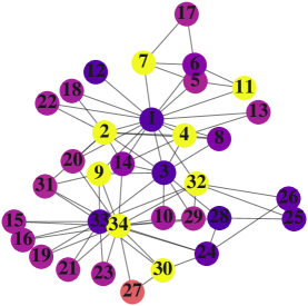
(a) $f(X)=23.2$
$X=\{2,4,7,9,11,30,32,34\}$

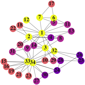
(b) $f(S^{(4)})=25.5$
$S^{(4)}=\{1,2,3,6,7,32,33,34\}$

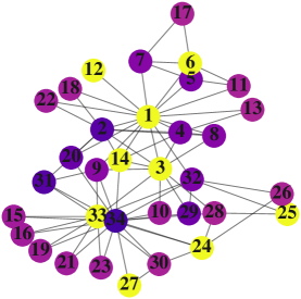
(c) $f(Y)=23.6$
$Y=\{1,3,6,14,24,25,27,33\}$

Figure 1. Example of influence maximization reconfiguration on karate network (see section 7.1). Each vertex is colored according to the activation probability. Given seed sets $X$ (1a) and $Y$ (1c), we wish to find a sequence of influential seed sets connecting them. The 4th seed set $S^{(4)}$ (1b) found by our algorithm (see section 5.2) is more influential than $X$ and $Y$.

Influence Maximization Reconfiguration (section 7.1): Suppose we are going to plan a viral marketing campaign (Domingos and Richardson, 2001) for promoting a company’s new product. Given structural data about a social network, we can solve influence maximization (Kempe et al., 2003) to identify a small group of influential users. However, the power of influence may decay as time goes by because social networks are evolving (Leskovec et al., 2007a; Ohsaka et al., 2016) or users may be affected by overexposure (Loukides et al., 2020). One strategy to circumvent this issue is replacing an outdated group with a newly-found one. When a change in user groups incurs a cost and we are given a limited budget (e.g., per day), we need to interpolate between an outdated group and a new one without significantly sacrificing the influence, which entails the concept of reconfiguration. Figure 1 depicts an example of influence maximization.

MAP Inference Reconfiguration (section 7.2): Consider that we are required to arrange a list of items to be displayed on a recommender system. If a feature vector is given for each item, we can use a determinantal point process (Borodin and Rains, 2005; Macchi, 1975) to extract a few items achieving a good balance between item quality and set diversity (Kulesza and Taskar, 2012; Gillenwater et al., 2012). Since novelty plays a crucial role in increasing the recommendation utility (Vargas and Castells, 2011), we would want to update the item list continuously. On the other hand, we need to ensure stability (Adomavicius and Zhang, 2012); i.e., the list should not be drastically changed over time, which gives rise to reconfiguration.

Source problems for both examples are formulated as Submodular Maximization (Nemhauser et al., 1978; Buchbinder and Feldman, 2018a, b; Krause and Golovin, 2014; Buchbinder et al., 2015), which finds many applications in data mining (see section 2). Unfortunately, the primary concern in the area of reconfiguration has been revealing the computational complexity of reconfiguration problems for classical problems such as graph-algorithmic problems and Boolean satisfiability (see section 2), which are incompatible with Data Mining and not applicable to the above examples. Our objective is to formulate, analyze, and apply reconfiguration problems derived from a submodular function.

1.1. Our Contributions

We present an initial, systematic study on reconfiguration problems on submodular functions. Our submodular reconfiguration problems request to determine whether there exists a solution sequence connecting two input solutions such that each solution has an objective value above a threshold in a submodular function $f:2^{[n]}\to\mathbb{R}_{+}$ and is obtained from the previous one by applying a simple transformation rule (e.g., a single element addition and removal). We formulate three submodular reconfiguration problems according to Ito et al. (2011)’s framework of reconfiguration:

• Monotone Submodular Reconfiguration (MSReco; Problem 3.2): This problem derives from Monotone Submodular Maximization and applies to influence maximization reconfiguration.

• Unconstrained Submodular Reconfiguration (USReco[tar] and USReco[tjar]; Problems 3.3 and 3.4): These problems derive from Unconstrained Submodular Maximization and two transformation rules. MAP inference reconfiguration fits into them.

We further formulate the optimization variants (Problems 3.5, 3.6 and 3.7), which aim to maximize the minimum objective value among the solutions in the output sequence. We analyze the proposed reconfiguration problems through the lens of computational complexity. Our complexity-theoretic results are summarized in Table 1.

Hardness (section 4)

We first investigate the computational tractability of the submodular reconfiguration problems. We prove that MSReco, USReco[tar], and USReco[tjar] are all PSPACE-complete (Theorems 4.2, 4.5 and 4.6), which is at least as hard as NP-completeness.

Approximability (section 5)

Having established the hardness of solving MSReco and USReco exactly, we seek for approximation in terms of the minimum function value in the output sequence; namely, we would like to maximize the minimum function value among the solutions as much as possible. We design a $\max\{\frac{1}{2},(1-\kappa)^{2}\}$-approximation algorithm for MSReco (Theorem 5.1), where $\kappa$ is the total curvature of a submodular function, and a $\frac{1}{n}$-approximation algorithm for USReco[tjar] (Theorem 5.3).

Inapproximability (section 6)

We further devise two hardness of approximation results. One is that approximating the optimum value of MSReco within a factor of $(1-\frac{1+\epsilon}{n^{2}})$ is PSPACE-hard (Theorem 6.1), implying that a fully polynomial-time approximation scheme does not exist assuming P $\neq$ PSPACE. The other is that we cannot find a $(\frac{5}{6}+\epsilon)$-approximation for USReco, without making a complexity-theoretic assumption. (Theorems 6.3 and 6.2).

Numerical Study (section 7)

We finally report numerical study on the reconfiguration version of influence maximization (Kempe et al., 2003) using network data and that of MAP inference on determinantal point process (Gillenwater et al., 2012) using movie rating data, which are formulated as MSReco and USReco[tjar], respectively. Comparing to an A* search algorithm, we observe that an approximation algorithm for MSReco quickly finds sequences that are better than the worst-case analysis, while that for USReco[tjar] is far worse than the optimal sequence.

2. Related Work

Reconfiguration Problems

The concept of reconfiguration has arisen in problems involving transformation and movement, such as the 15-puzzle (Johnson and Story, 1879) and the Rubik’s Cube. Ito et al. (2011) established the unified framework of reconfiguration. One of the most important reconfiguration problems is reachability, asking to decide the existence of a solution sequence between two feasible solutions for a particular source problem. Countless source problems derive the respective reconfiguration problems in Ito et al. (2011)’s framework, including graph-algorithmic problems, Boolean satisfiability, and others; revealing their computational complexity has been the primary concern in Theoretical Computer Science. Typically, an NP-complete source problem brings a PSPACE-complete reachability problem, e.g., Vertex Cover (Kamiński et al., 2012), Set Cover (Ito et al., 2011), 4-Coloring (Bonsma and Cereceda, 2009), Clique (Ito et al., 2011), and 3-SAT (Gopalan et al., 2009). On the other hand, a source problem in P usually induces a reachability problem in P, e.g., Matching (Ito et al., 2011) and 2-SAT (Gopalan et al., 2009). However, some exceptions are known; e.g., 3-Coloring is NP-complete, but its reachability version is in P (Johnson et al., 2016). See Nishimura (2018)’s survey for more information. This study explores reconfiguration problems for which the source problem is Submodular Maximization, which generalizes Vertex Cover and Set Cover and has more of a flavor of Data Mining.

Submodular Function Maximization

We review two submodular function maximization problems, which have been studied in Theoretical Computer Science and applied in Data Mining.

Given a monotone submodular function, Monotone Submodular Maximization requires finding a fixed-size set having the maximum function value. The simple greedy algorithm has a provable guarantee of returning a $(1-1/\mathrm{e})$-factor approximation in polynomial time (Nemhauser et al., 1978). This factor is the best possible as no polynomial-time algorithm can achieve a better approximation factor (Nemhauser and Wolsey, 1978; Feige, 1998). Since monotone submodular functions abide by the law of diminishing returns, Monotone Submodular Maximization has been applied to a diverse range of data mining tasks, e.g., influence maximization (Kempe et al., 2003) document summarization (Lin and Bilmes, 2011), outbreak detection (Leskovec et al., 2007b), and sensor placement (Krause et al., 2008). We develop a $\frac{1}{2}$-approximation algorithm for the corresponding reconfiguration problem (section 5.2).

Given a (not necessarily monotone) submodular function, Unconstrained Submodular Maximization requires finding a subset that maximizes the function value. This problem can be approximated within a $\frac{1}{2}$-factor (Buchbinder et al., 2015; Buchbinder and Feldman, 2018a), which is proven to be optimal (Feige et al., 2011). Some of the application tasks include movie recommendation, image summarization (Mirzasoleiman et al., 2016), and MAP inference on determinantal point process (Gillenwater et al., 2012). We develop a $\frac{1}{n}$-approximation algorithm for the corresponding reconfiguration problem (section 5.3).

3. Problem Formulation

Preliminaries

For a nonnegative integer $n$, let $[n]\triangleq\{1,2,\ldots,n\}$. $\mathbb{R}_{+}$ represents the set of nonnegative real numbers. For a finite set $S$ and a nonnegative integer $k$, we write ${S\choose k}$ for the family of all size-$k$ subsets of $S$. A sequence $\mathcal{S}$ consisting of a finite number of sets $S^{(0)},S^{(1)},\ldots,S^{(\ell)}$ is denoted as $\langle S^{(0)},S^{(1)},\ldots,S^{(\ell)}\rangle$, and we write $S^{(i)}\in\mathcal{S}$ to mean that $S^{(i)}$ appears in $\mathcal{S}$ (at least once). The symbol $\uplus$ is used to emphasize that the union is taken over two disjoint sets. Throughout this paper, we assume that every set function is nonnegative. For a set function $f:2^{[n]}\to\mathbb{R}_{+}$, we say that $f$ is monotone if $f(S)\leq f(T)$ for all $S\subseteq T\subseteq[n]$, $f$ is modular if $f(S)+f(T)=f(S\cap T)+f(S\cup T)$ for all $S,T\subseteq[n]$, and $f$ is submodular if $f(S)+f(T)\geq f(S\cap T)+f(S\cup T)$ for all $S,T\subseteq[n]$. Submodularity is known to be equivalent to the following diminishing returns property (Schrijver, 2003): $f(S\cup\{e\})-f(S)\geq f(T\cup\{e\})-f(T)$ for all $S\subseteq T\subseteq[n]$ and $e\in[n]\setminus T$. For a subset $R\subseteq[n]$, the residual (Krause and Golovin, 2014) is defined as a set function $f_{R}:2^{[n]\setminus R}\to\mathbb{R}_{+}$ such that $f_{R}(S)\triangleq f(S\uplus R)-f(R)$ for $S\subseteq[n]\setminus R$. If $f$ is monotone and submodular, then so is $f_{R}$ (Krause and Golovin, 2014). The total curvature $\kappa$ (Conforti and Cornuéjols, 1984; Vondrák, 2010) of a monotone submodular function $f:2^{[n]}\to\mathbb{R}_{+}$ is defined as $\kappa\triangleq 1-\min_{e\in[n]}\frac{f([n])-f([n]\setminus\{e\})}{f(\{e\})}.$ The total curvature $\kappa$ takes a value from $0$ to $1$, which captures how far away $f$ is from being modular; e.g., a modular function has curvature $\kappa=0$, and a coverage function has curvature $\kappa=1$. We assume to be given access to a value oracle for a set function $f$, which returns $f(S)$ whenever it is called with a query $S$. We recall the definitions of two submodular function maximization problems:

• Monotone Submodular Maximization: Given a monotone submodular function $f:2^{[n]}\to\mathbb{R}_{+}$ and a solution size $k$, maximize $f(S)$ subject to $S\in{[n]\choose k}$.

• Unconstrained Submodular Maximization: Given a submodular function $f:2^{[n]}\to\mathbb{R}_{+}$, maximize $f(S)$ subject to $S\subseteq[n]$.

3.1. Ito et al. (2011)’s Reconfiguration Framework

In reconfiguration problems, we wish to determine whether there exists a sequence of solutions between a pair of solutions for a particular “source” problem such that each is “feasible” and obtained from the previous one by applying a simple “transformation rule.” We recapitulate the reconfiguration framework of Ito et al. (2011). The reconfiguration framework requires three ingredients (Nishimura, 2018; Ito et al., 2011; Mouawad, 2015):

• a source problem, which is usually a search problem in P or NP-complete;

• a definition of feasible solutions;

• an adjacency relation over the pairs of two solutions, typically symmetric and polynomial-time testable (Nishimura, 2018).

An adjacency relation can be defined in terms of a reconfiguration step, which specifies how a solution can be transformed. We say that two solutions are adjacent if one can be transformed into the other by applying a single reconfiguration step. We now define a central concept called reconfiguration sequences.

Definition 3.1.

For two feasible solutions $X$ and $Y$, a reconfiguration sequence from $X$ to $Y$ is a sequence of feasible solutions $\mathcal{S}=\langle S^{(0)},S^{(1)},\ldots,S^{(\ell)}\rangle$ starting from $X$ (i.e., $S^{(0)}=X$) and ending with $Y$ (i.e., $S^{(\ell)}=Y$) such that every two consecutive solutions $S^{(i-1)}$ and $S^{(i)}$ for $i\in[\ell]$ are adjacent (i.e., $S^{(i)}$ is obtained from $S^{(i-1)}$ by a single reconfiguration step). The length $\ell$ of $\mathcal{S}$ is defined as the number of (possibly duplicate) solutions in it minus $1$.

There are several types of reconfiguration problems (Nishimura, 2018; Mouawad, 2015; van den Heuvel, 2013). One of the most important problems is reachability, asking to determine whether there exists a reconfiguration sequence between a pair of feasible solutions. Of course, reconfiguration problems for the same source problem can have different complexities depending on the definitions of feasibility and adjacency.

3.2. Defining Submodular Reconfiguration

We are now ready to formulate reconfiguration problems on submodular functions. We first designate the ingredients required for defining the reconfiguration framework. Source problems are either Monotone Submodular Maximization or Unconstrained Submodular Maximization. Given a submodular function $f:2^{[n]}\to\mathbb{R}_{+}$, we define the feasibility according to (Ito et al., 2011, §2.2): We introduce a threshold $\theta$, offering a lower bound on the allowed function values, and a set $S$ is said to be feasible if $f(S)\geq\theta$. For a set sequence $\mathcal{S}$, the value of $\mathcal{S}$, denoted $f(\mathcal{S})$, is defined as the minimum function value among all sets in $\mathcal{S}$, i.e., $f(\mathcal{S})\triangleq\min_{S^{(i)}\in\mathcal{S}}f(S^{(i)})$. Accordingly, a reconfiguration sequence $\mathcal{S}$ must satisfy $f(\mathcal{S})\geq\theta$. We consider three reconfiguration steps to specify an adjacency relation, some of which are established in the literature:

• Token jumping (tj) (Kamiński et al., 2012): Given a set, a tj step can remove one element from it and add another element not in it at the same time; i.e., two sets are adjacent under tj if they have the same size and their intersection has a size one less than their size.

• Token addition or removal (tar) (Ito et al., 2011): Given a set, a tar step can remove an element from it or add an element not in it; i.e., two sets are adjacent under tar if the symmetric difference has size $1$.

• Token jumping, addition, or removal (tjar): A tjar step can perform either a tj or tar step.

It is easy to see that these adjacency relations are symmetric and polynomial-time testable.

3.2.1. Reachability Problems

We define three reachability problems on a submodular function with different adjacency relations.

Problem 3.2 (Monotone Submodular Reconfiguration; MSReco).

Given a monotone submodular function $f:2^{[n]}\to\mathbb{R}_{+}$, two sets $X$ and $Y$ in ${[n]\choose k}$, and a threshold $\theta$, decide if there exists a reconfiguration sequence $\mathcal{S}$ from $X$ to $Y$ under tj such that $f(\mathcal{S})\geq\theta$.

Problem 3.3 (Unconstrained Submodular Reconfiguration in tar; USReco[tar]).

Given a submodular function $f:2^{[n]}\to\mathbb{R}_{+}$, two subsets $X$ and $Y$ of $[n]$, and a threshold $\theta$, decide if there exists a reconfiguration sequence $\mathcal{S}$ from $X$ to $Y$ under tar such that $f(\mathcal{S})\geq\theta$.

Problem 3.4 (Unconstrained Submodular Reconfiguration in tjar; USReco[tjar]).

Given a submodular function $f:2^{[n]}\to\mathbb{R}_{+}$, two subsets $X$ and $Y$ of $[n]$, and a threshold $\theta$, decide if there exists a reconfiguration sequence $\mathcal{S}$ from $X$ to $Y$ under tjar such that $f(\mathcal{S})\geq\theta$.

Note that these problems do not request an actual reconfiguration sequence. Without loss of generality, we assume that $\theta$ is at most $\min\{f(X),f(Y)\}$, because otherwise the answer is always “no.”

3.2.2. Optimization Variants

By definition, the answer to Problems 3.2, 3.3 and 3.4 is always “yes” if $\theta=0$. On the other hand, there exists a constant $\theta_{\mathrm{yes}}$, referred to as a reconfiguration index (Ito et al., 2016), for which the answer is “yes” if $\theta\leq\theta_{\mathrm{yes}}$ and “no” otherwise. We can thus think of the following optimization variants, requiring that $f(\mathcal{S})$ be maximized among all possible reconfiguration sequences. Such variants have been studied for Clique (Ito et al., 2011) and Subset Sum (Ito and Demaine, 2014).

Problem 3.5 (Maximum Monotone Submodular Reconfiguration; MaxMSReco).

Given a monotone submodular function $f:2^{[n]}\to\mathbb{R}_{+}$ and two sets $X$ and $Y$ in ${[n]\choose k}$, find a reconfiguration sequence $\mathcal{S}$ from $X$ to $Y$ under tj maximizing $f(\mathcal{S})$.

Problem 3.6 (Maximum Unconstrained Submodular Reconfiguration in tar; MaxUSReco[tar]).

Given a submodular function $f:2^{[n]}\to\mathbb{R}_{+}$ and two subsets $X$ and $Y$ of $[n]$, find a reconfiguration sequence $\mathcal{S}$ from $X$ to $Y$ under tar maximizing $f(\mathcal{S})$.

Problem 3.7 (Maximum Unconstrained Submodular Reconfiguration in tjar; MaxUSReco[tjar]).

Given a submodular function $f:2^{[n]}\to\mathbb{R}_{+}$ and two subsets $X$ and $Y$ of $[n]$, find a reconfiguration sequence $\mathcal{S}$ from $X$ to $Y$ under tjar maximizing $f(\mathcal{S})$.

4. Hardness

In this section, we prove that MSReco, USReco[tar], and USReco[tjar] are all PSPACE-complete to solve (Theorems 4.2, 4.5 and 4.6). Here, PSPACE is a class of decision problems that can be solved using polynomial space in the input size, and a decision problem is said to be PSPACE-complete if it is in PSPACE and every problem in PSPACE can be reduced to it in polynomial time. PSPACE is known to include (and believed to be outside (Arora and Barak, 2009)) P, NP, and $\sharp$P. Commonly known PSPACE-complete problems are Quantified Boolean Formula (Garey and Johnson, 1979), puzzles and games such as Sliding Blocks (Hearn and Demaine, 2005) and Go (Lichtenstein and Sipser, 1980). We can easily verify that submodular reconfiguration problems are included in PSPACE, whose proof is deferred to Appendix A.

Observation 4.1.

Problems 3.2, LABEL:, 3.3, LABEL: and 3.4 are in PSPACE.

4.1. PSPACE-completeness of MSReco

Theorem 4.2.

MSReco is PSPACE-complete.

To prove Theorem 4.2, we use a polynomial-time reduction from Minimum Vertex Cover Reconfiguration. Of a graph, a vertex cover is a set of vertices that include at least one endpoint of every edge of the graph. Given a graph and an integer $k$, it is NP-complete to decide if there exists a vertex cover of size $k$ (Karp, 1972). We define Minimum Vertex Cover Reconfiguration as follows.

Problem 4.3 (Minimum Vertex Cover Reconfiguration).

Given a graph $G=(V,E)$ and two minimum vertex covers $C^{x}$ and $C^{y}$ of the same size, determine whether there exists a sequence of minimum vertex covers from $C^{x}$ to $C^{y}$ under tj.

Our definition is different from that of Vertex Cover Reconfiguration due to (Ito et al., 2011; Ito et al., 2016), in which two input vertex covers may not be minimum. We show that Problem 4.3 is PSPACE-hard, whose proof is reminiscent of (Ito et al., 2011, Theorem 2) and deferred to Appendix A.

Lemma 4.4.

Problem 4.3 is PSPACE-hard.

Proof of Theorem 4.2.

We present a polynomial-time reduction from Minimum Vertex Cover Reconfiguration. Suppose we are given a graph $G=(V,E)$ and two minimum vertex covers $C^{x}$ and $C^{y}$. Define a set function $f:2^{V}\to\mathbb{R}_{+}$ such that $f(S)$ for $S\subseteq V$ is the number of edges in $E$ that are incident to $S$. In particular, $f(S)=|E|$ if and only if $S$ is a vertex cover of $G$. Since $f$ is monotone and submodular, we construct an instance of MSReco consisting of $f$, $C^{x}$, $C^{y}$, and a threshold $|E|$. Observe that a reconfiguration sequence for the Minimum Vertex Cover Reconfiguration instance is a reconfiguration sequence for the MSReco instance, and vice versa, which completes the reduction. ∎

4.2. PSPACE-completeness of USReco

Theorem 4.5.

USReco[tar] is PSPACE-complete.

Proof.

We demonstrate a polynomial-time reduction from Monotone Not-All-Equal 3-SAT Reconfiguration, which is PSPACE-complete (Cardinal et al., 2020). A 3-conjunctive normal form (3-CNF) formula $\phi$ is said to be monotone if no clause contains negative literals (e.g., $\phi=(x_{1}\vee x_{2}\vee x_{3})\wedge(x_{2}\vee x_{3}\vee x_{4})\wedge(x_{1}\vee x_{3}\vee x_{4})$). We assume that every clause of $\phi$ contains exactly three literals. We say that a truth assignment $\mathbf{\bm{\sigma}}$ not-all-equal satisfies $\phi$ if every clause contains exactly two literals with the same value; i.e., it contains at least one true literal and at least one false literal (e.g., $\mathbf{\bm{\sigma}}(x_{1})=\mathbf{\bm{\sigma}}(x_{2})=\mathbf{\bm{\sigma}}(x_{4})=\textsf{True}$ and $\mathbf{\bm{\sigma}}(x_{3})=\textsf{False}$). In Monotone Not-All-Equal 3-SAT Reconfiguration, given a monotone 3-CNF formula $\phi$ and two not-all-equal satisfying truth assignments $\mathbf{\bm{\sigma}}^{x}$ and $\mathbf{\bm{\sigma}}^{y}$ of $\phi$, we wish to determine whether there exists a sequence of not-all-equal satisfying truth assignments of $\phi$ between $\mathbf{\bm{\sigma}}^{x}$ and $\mathbf{\bm{\sigma}}^{y}$ such that each truth assignment is obtained from the previous one by a single variable flip; i.e., they differ in exactly one variable (cf. 3-SAT Reconfiguration (Gopalan et al., 2009) in Problem A.1).

Suppose we are given a monotone 3-CNF formula $\phi$ with $n$ variables $x_{1},\ldots,x_{n}$ and $m$ clauses $c_{1},\ldots,c_{m}$ and two not-all-equal satisfying truth assignments $\mathbf{\bm{\sigma}}^{x}$ and $\mathbf{\bm{\sigma}}^{y}$ of $\phi$. For a subset $S\subseteq[n]$, we write $\mathbf{\bm{\sigma}}_{S}$ for a truth assignment such that $\mathbf{\bm{\sigma}}_{S}(x_{i})$ for variable $x_{i}$ is True if $i\in S$ and False otherwise. For a truth assignment $\mathbf{\bm{\sigma}}$, we define the set $S_{\mathbf{\bm{\sigma}}}\triangleq\{i\in[n]\mid\mathbf{\bm{\sigma}}(x_{i})=\textsf{True}\}$. We now construct a set function $f_{\phi}:2^{[n]}\to\mathbb{R}_{+}$ such that $f(S)$ for $S\subseteq[n]$ is the number of clauses not-all-equal satisfied by $\mathbf{\bm{\sigma}}_{S}$. In particular, $f(S)=m$ if $\mathbf{\bm{\sigma}}_{S}$ not-all-equal satisfies $\phi$. Since $f$ is submodular, we construct an instance of USReco consisting of $f$, $S_{\mathbf{\bm{\sigma}}^{x}}$, $S_{\mathbf{\bm{\sigma}}^{y}}$, and a threshold $m$. Observe that there exists a reconfiguration sequence for the Monotone Not-All-Equal 3-SAT Reconfiguration instance if and only if there exists a reconfiguration sequence for the USReco instance, which completes the reduction. ∎

The last PSPACE-completeness result is shown below, whose proof is based on a reduction from Minimum Vertex Cover Reconfiguration and deferred to Appendix A.

Theorem 4.6.

USReco[tjar] is PSPACE-complete.

Algorithm 1 Greedy algorithm.

1:function $f:2^{[n]}\to\mathbb{R}_{+}$; set $N\subseteq[n]$; solution size $k\leq|N|$.

2:for each $i=1\;\textbf{to}\;k$ do $\displaystyle e_{i}\leftarrow\operatorname*{arg\,max}_{e\in N\setminus\{e_{1},\ldots,e_{i-1}\}}f(\{e_{1},\ldots,e_{i-1},e\})$.

3:return sequence $\langle e_{1},\ldots,e_{k}\rangle$.

5. Approximability

In the previous section, we saw that MSReco, USReco[tar], and USReco[tjar] are all PSPACE-complete, implying that their optimization variants are also hard to solve exactly in polynomial time. However, there is still room for consideration of approximability. A $\rho$-approximation algorithm for $\rho\leq 1$ is a polynomial-time algorithm that returns a reconfiguration sequence $\mathcal{S}$ such that $f(\mathcal{S})\geq\rho\cdot f(\mathcal{S}^{*})$, where $\mathcal{S}^{*}$ is an optimal reconfiguration sequence with the maximum value. We design a $\max\{\frac{1}{2},(1-\kappa)^{2}\}$-approximation algorithm for MaxMSReco (section 5.2; Theorem 5.1), where $\kappa$ is the total curvature, and a $\frac{1}{n}$-approximation algorithm for MaxUSReco[tjar] (section 5.3; Theorem 5.3), while we explain the difficulty in algorithm development for MaxUSReco[tar] (section 5.4).

5.1. Greedy Algorithm

Before going into details of the proposed algorithms, we introduce the greedy algorithm shown in Algorithm 1, which is used as a subroutine. Given a set function $f:2^{[n]}\to\mathbb{R}_{+}$, a ground set $N\subseteq[n]$, and a solution size $k\leq|N|$, the greedy algorithm iteratively selects an element of $N$, not having been chosen so far, that maximizes the function value. The number of calls to a value oracle of $f$ is at most $|N|k$. Let $e_{i}$ denote an element chosen at the $i$-th iteration; define $S_{i}\triangleq\{e_{1},\ldots,e_{i}\}$. We call the output sequence $\langle e_{1},\ldots,e_{k}\rangle$ a greedy sequence. If $f$ is a submodular function, then the following inequality is known to hold for any $1\leq i\leq j\leq k$, see, e.g., (Krause and Golovin, 2014):

(1) $$f(S_{i})-f(S_{i-1})\geq f(S_{j})-f(S_{j-1}).$$

5.2. $\max\{\frac{1}{2},(1-\kappa)^{2}\}$-Approximation Algorithm for MaxMSReco

Algorithm 2 describes the proposed approximation algorithm for MaxMSReco. Given a monotone submodular function $f:2^{[n]}\to\mathbb{R}_{+}$ and two sets $X$ and $Y$ in ${[n]\choose k}$, it first invokes Algorithm 1 on $f_{R}$, $X\setminus R$, and $k^{\prime}$ (resp. $f_{R}$, $Y\setminus R$, and $k^{\prime}$), where $R\triangleq X\cap Y$ and $k^{\prime}\triangleq|X\setminus R|=|Y\setminus R|$, to obtain a greedy sequence $\langle x_{1},\ldots,x_{k^{\prime}}\rangle$ (resp. $\langle y_{1},\ldots,y_{k^{\prime}}\rangle$). It then returns a set sequence from $X$ to $Y$, the $i$-th set in which is defined as $S^{(i)}\triangleq\{x_{1},\ldots,x_{k^{\prime}-i}\}\uplus\{y_{1},\ldots,y_{i}\}\uplus R$. Our algorithm is guaranteed to return a $\max\{\frac{1}{2},(1-\kappa)^{2}\}$-approximation reconfiguration sequence in $\mathcal{O}(nk)$ time, where $\kappa$ is the total curvature of $f$. Algorithm 2 is thus nearly optimal whenever $\kappa\approx 0$. Such a small $\kappa$ can be observed in real-world problems, e.g., entropy sampling on Gaussian radial basis function kernels (Sharma et al., 2015).

Algorithm 2 $\max\{\frac{1}{2},(1-\kappa)^{2}\}$-approximation algorithm for MaxMSReco.

1:monotone submodular func. $f:2^{[n]}\to\mathbb{R}_{+}$; two sets $X,Y\in{[n]\choose k}$.

2:$R\leftarrow X\cap Y,\quad X^{\prime}\leftarrow X\setminus R,\quad Y^{\prime}\leftarrow Y\setminus R,\quad k^{\prime}\leftarrow|X^{\prime}|=|Y^{\prime}|$.

3:invoke Algorithm 1 on $f_{R},X^{\prime},k^{\prime}$ to get greedy sequence $\langle x_{1},\ldots,x_{k^{\prime}}\rangle$.

4:invoke Algorithm 1 on $f_{R},Y^{\prime},k^{\prime}$ to get greedy sequence $\langle y_{1},\ldots,y_{k^{\prime}}\rangle$.

5:for each $i=0\;\textbf{to}\;k^{\prime}$ do $S^{(i)}\leftarrow\{x_{1},\ldots,x_{k^{\prime}-i}\}\uplus\{y_{1},\ldots,y_{i}\}\uplus R$.

6:return sequence $\mathcal{S}=\langle S^{(0)},\ldots,S^{(k^{\prime})}\rangle$.

Theorem 5.1.

Given a monotone submodular function $f:2^{[n]}\to\mathbb{R}_{+}$ and two sets $X$ and $Y$ in ${[n]\choose k}$, Algorithm 2 returns a reconfiguration sequence $\mathcal{S}$ for MaxMSReco of length at most $k$ in $\mathcal{O}(nk)$ time such that $f(\mathcal{S})\geq\max\{\frac{1}{2},(1-\kappa)^{2}\}\min\{f(X),f(Y)\}$. In particular, it is a $\max\{\frac{1}{2},(1-\kappa)^{2}\}$-approximation algorithm for MaxMSReco.

Proof.

Define $R\triangleq X\cap Y$, $X^{\prime}\triangleq X\setminus R$, $Y^{\prime}\triangleq Y\setminus R$, and $k^{\prime}\triangleq|X^{\prime}|=|Y^{\prime}|$. Let $\langle x_{1},\ldots,x_{k^{\prime}}\rangle$ (resp. $\langle y_{1},\ldots,y_{k^{\prime}}\rangle$) denote the greedy sequence returned by Algorithm 1 invoked on $f_{R},X^{\prime},k^{\prime}$ (resp. $f_{R},Y^{\prime},k^{\prime}$). For each $i\in\{0\}\cup[k^{\prime}]$, we define $X_{i}\triangleq\{x_{1},\ldots,x_{i}\}$ and $Y_{i}\triangleq\{y_{1},\ldots,y_{i}\}$. Note that $X_{0}=Y_{0}=\emptyset$, $X_{k^{\prime}}=X^{\prime}$, and $Y_{k^{\prime}}=Y^{\prime}$. For each $i\in\{0\}\cup[k^{\prime}]$, $S^{(i)}$ in the returned reconfiguration sequence $\mathcal{S}$ is equal to $X_{k^{\prime}-i}\uplus Y_{i}\uplus R$, which is of size $k$. The correctness of Algorithm 2 comes from the fact that $S^{(i)}$ is obtained from $S^{(i-1)}$ by removing $x_{k^{\prime}-i+1}$ and adding $y_{i}$. The time complexity is apparent.

Showing that $f(S^{(i)})\geq\frac{1}{2}\min\{f(X),f(Y)\}$ for every $i$ now suffices to prove a $\frac{1}{2}$-approximation. Since the statement is clear if $i=0,k^{\prime}$, we will prove for the case of $i\in[k^{\prime}-1]$. Observe first that, whenever $i\leq j$, we have that $f_{R}(X_{i})-f_{R}(X_{i-1})\geq f_{R}(X_{j})-f_{R}(X_{j-1})$ due to Eq. 1. Hence, for any $i\in[k^{\prime}-1]$, we have that

$$\tfrac{1}{i}{\textstyle\sum\limits_{1\leq j\leq i}}(f_{R}(X_{j})-f_{R}(X_{j-1}))\geq\tfrac{1}{k^{\prime}-i}{\textstyle\sum\limits_{i+1\leq j\leq k^{\prime}}}(f_{R}(X_{j})-f_{R}(X_{j-1})).$$

Simple calculation further yields that $f_{R}(X_{i})\geq\frac{i}{k^{\prime}}f_{R}(X^{\prime})$, where we have used the nonnegativity of $f_{R}(\emptyset)$. Similarly, we can show that $f_{R}(Y_{i})\geq\frac{i}{k^{\prime}}f_{R}(Y^{\prime})$ for every $i\in[k^{\prime}-1]$. Using the two inequalities on $f_{R}(X_{k^{\prime}-i})$ and $f_{R}(Y_{i})$, we have that for any $i\in[k^{\prime}-1]$,

$$f(S^{(i)})=f_{R}(X_{k^{\prime}-i}\uplus Y_{i})+f(R)\geq\max\{f_{R}(X_{k^{\prime}-i}),f_{R}(Y_{i})\}+f(R)$$

(2) $$\geq\max\bigl{\{}\tfrac{k^{\prime}-i}{k^{\prime}}f_{R}(X^{\prime}),\tfrac{i}{k^{\prime}}f_{R}(Y^{\prime})\bigr{\}}+f(R)=\tfrac{1}{2}\min\{f(X),f(Y)\},$$

where the first inequality is due to the monotonicity of $f_{R}$. Proving a $(1-\kappa)^{2}$-approximation is deferred to Appendix A. ∎

Difficult Instance for Algorithm 2

We provide a specific instance of MaxMSReco for which Algorithm 2 returns a $\frac{3}{4}$-approximation reconfiguration sequence, whose proof is deferred to Appendix A. As a by-product, we give evidence that an optimal reconfiguration sequence can include elements outside $X\cup Y$.

Observation 5.2.

There exists an instance $f,X,Y$ of MaxMSReco such that the optimal reconfiguration sequence $\mathcal{S}^{*}$ has value $f(\mathcal{S}^{*})=1$, and any reconfiguration sequence $\mathcal{S}$ that is restricted to include only subsets of $X\cup Y$ has value $f(\mathcal{S})\leq\frac{3}{4}$. Thus, Algorithm 2 returns a $\frac{3}{4}$-approximation reconfiguration sequence for this instance.

5.3. $\frac{1}{n}$-Approximation Algorithm for MaxUSReco[tjar]

Algorithm 3 $\frac{1}{n}$-approximation algorithm for MaxUSReco[tjar].

1:submodular function $f:2^{[n]}\to\mathbb{R}_{+}$; two subsets $X,Y$ of $[n]$.

2:invoke Algorithm 1 on $f,X,|X|$ to get greedy sequence $\langle x_{1},\ldots,x_{|X|}\rangle$.

3:invoke Algorithm 1 on $f,Y,|Y|$ to get greedy sequence $\langle y_{1},\ldots,y_{|Y|}\rangle$.

4:declare empty sequence $\mathcal{S}=\langle\rangle$.

5:for each $i=|X|\;\textbf{to}\;1$ do append $\{x_{1},\ldots,x_{i}\}$ at the end of $\mathcal{S}$.

6:for each $i=1\;\textbf{to}\;|Y|$ do append $\{y_{1},\ldots,y_{i}\}$ at the end of $\mathcal{S}$.

7:return sequence $\mathcal{S}$.

Algorithm 3 describes the proposed approximation algorithm for MaxUSReco[tjar]. Given a submodular function $f:2^{[n]}\to\mathbb{R}_{+}$ and two subsets $X$ and $Y$ of $[n]$, it first invokes Algorithm 1 on $f,X,|X|$ and $f,Y,|Y|$ to obtain the greedy sequences $\langle x_{1},\ldots,x_{|X|}\rangle$ and $\langle y_{1},\ldots,y_{|Y|}\rangle$, respectively. It then returns the concatenation of a reconfiguration sequence from $X$ to $\{x_{1}\}$ and that from $\{y_{1}\}$ to $Y$. Our algorithm is guaranteed to return a $\frac{1}{n}$-approximation reconfiguration sequence in $\mathcal{O}(n^{2})$ time as claimed below.

Theorem 5.3.

Given a submodular function $f:2^{[n]}\to\mathbb{R}_{+}$ and two subsets $X$ and $Y$ of $[n]$, Algorithm 3 returns a reconfiguration sequence $\mathcal{S}$ for MaxUSReco[tjar] of length at most $2n$ in $\mathcal{O}(n^{2})$ time such that $f(\mathcal{S})\geq\frac{1}{n}\min\{f(X),f(Y)\}$. In particular, it is a $\frac{1}{n}$-approximation algorithm for MaxUSReco[tjar].

Proof.

Let $\langle x_{1},\ldots,x_{|X|}\rangle$ (resp. $\langle y_{1},\ldots,y_{|Y|}\rangle$) denote the greedy sequence returned by Algorithm 1 invoked on $f,X,|X|$ (resp. $f,Y,|Y|$). For each $i\in\{0\}\cup[|X|]$ (resp. $i\in\{0\}\cup[|Y|]$), we define $X_{i}\triangleq\{x_{1},\ldots,x_{i}\}$ (resp. $Y_{i}\triangleq\{y_{1},\ldots,y_{i}\}$). Observe that the sequence $\mathcal{S}$ returned by Algorithm 3 is a valid reconfiguration sequence for MaxUSReco[tjar] and consists of sets in the form of either $X_{i}$ or $Y_{i}$ for some $i\geq 1$. The time complexity is obvious.

We will show that $f(X_{i})\geq\frac{1}{|X|}f(X)$ for every $i\geq 1$. Since the value of $f(X_{i})-f(X_{i-1})$ is monotonically nonincreasing in $i\in[|X|]$ owing to Eq. 1, there exists an index $i^{*}$ such that $f(X_{i})-f(X_{i-1})\geq 0$ if $i\leq i^{*}$ and $f(X_{i})-f(X_{i-1})\leq 0$ if $i\geq i^{*}+1$. In the former case, we have that $f(X_{i})\geq f(X_{1});$ in the latter case, we have that $f(X_{i})\geq f(X).$ Using the inequality that $f(X)\leq\sum_{i\in[|X|]}f(\{x_{i}\})\leq|X|\cdot f(\{x_{1}\})$, we obtain that $f(X_{i})\geq\min\{f(X_{1}),f(X)\}\geq\frac{1}{|X|}f(X)$ for any $i\in[|X|]$. Similarly, we can derive an analogous inequality that for any $i\in[|Y|]$, $f(Y_{i})\geq\frac{1}{|Y|}f(Y).$ Accordingly, we derive that

(3) $$f(\mathcal{S})\geq\min\bigl{\{}\tfrac{1}{|X|}f(X),\tfrac{1}{|Y|}f(Y)\bigr{\}}\geq\tfrac{1}{n}\min\{f(X),f(Y)\},$$

which completes the proof. ∎

Does Algorithm 2 Work on MaxUSReco[tjar]?

Algorithm 3’s approximation factor of $\frac{1}{n}$ is not fascinating compared to a $\frac{1}{2}$-factor of Algorithm 2 on MaxMSReco. One might wonder if Algorithm 2 generates a good reconfiguration sequence on MaxUSReco[tjar], assuming that $|X|=|Y|$. However, we have bad news that Algorithm 2 does not have any positive approximation factor for MaxUSReco[tjar], whose proof is deferred to Appendix A.

Observation 5.4.

There exists an instance $f,X,Y$ of MaxUSReco[tjar] with $|X|=|Y|$ such that Algorithm 3 and Algorithm 2 return a reconfiguration sequence of value $1$ and $0$, respectively.

5.4. Difficulty in Designing Approximation Algorithms for MaxUSReco[tar]

Unfortunately, Algorithm 3 designed for MaxUSReco[tjar] does not produce a reconfiguration sequence for MaxUSReco[tar] because we cannot transform from $\{x_{1}\}$ to $\{y_{1}\}$ directly by a tar step. Here, we explain what makes it so challenging to design approximation algorithms for MaxUSReco[tar]. Eqs. 2 and 3 in the proofs of Theorems 5.1 and 5.3 indicate that if $f(X)$ and $f(Y)$ are positive, then there must exist a reconfiguration sequence $\mathcal{S}$ whose value is positive (which can be found efficiently). Such a feature is critical for proving $f(\mathcal{S})\geq\rho\cdot\min\{f(X),f(Y)\}$ for some positive $\rho>0$. We show, however, that this is not the case for MaxUSReco[tar]; i.e., it can be impossible to transform from $X$ to $Y$ without ever touching zero-value sets, whose proof is deferred to Appendix A.

Observation 5.5.

There exists an instance $f,X,Y$ of MaxUSReco[tar] such that $f(X)=f(Y)=1$ and every reconfiguration sequence $\mathcal{S}$ has value $f(\mathcal{S})=0$.

6. Inapproximability

In this section, we devise inapproximability results of MaxMSReco and MaxUSReco, which reveal an upper bound of approximation guarantees that polynomial-time algorithms can achieve. We first prove that it is PSPACE-hard to approximate the optimal value of MaxMSReco within a factor of $(1-\frac{1+\epsilon}{n^{2}})$ (section 6.1; Theorem 6.1), which is slightly stronger than Theorem 4.2. Though this factor asymptotically approaches $1$ (as $n$ goes to infinity), the result rules out the existence of a fully polynomial-time approximation scheme, assuming that P $\neq$ PSPACE (which is a weaker assumption than P $\neq$ NP). A fully polynomial-time approximation scheme (FPTAS) is an approximation algorithm that takes a precision parameter $\epsilon>0$ and returns a $(1-\epsilon)$-approximation in polynomial time in the input size and $\epsilon^{-1}$. We then show that both versions of MaxUSReco cannot be approximated within a factor of $(\frac{5}{6}+\epsilon)$ for any $\epsilon>0$ by using exponentially many oracle calls in $n$ and $\epsilon$, without making a complexity-theoretic assumption (section 6.2; Theorems 6.2 and 6.3).

6.1. Inapproximability Result of MaxMSReco

The first result is shown below, whose proof appears in Appendix A.

Theorem 6.1.

It is PSPACE-hard to approximate the optimal value of MaxMSReco within a factor of $(1-\frac{1+\epsilon}{n^{2}})$ for any $\epsilon>0$, where $n$ is the size of the ground set. In particular, an FPTAS for MaxMSReco does not exist unless P $=$ PSPACE.

6.2. Inapproximability Results of MaxUSReco

Theorem 6.2.

For any $\epsilon>0$, there is no $(\frac{5}{6}+\epsilon)$-approximation algorithm for MaxUSReco[tjar] making at most $\mathrm{e}^{\epsilon^{2}n/2}$ oracle calls.

Proof.

We show a reduction from Unconstrained Submodular Maximization in an approximation-preserving manner. Suppose we are given a submodular function $f:2^{[n]}\to\mathbb{R}_{+}$ and a number $\epsilon>0$, and we wish to find a $(\frac{1}{2}+\epsilon)$-approximation for Unconstrained Submodular Maximization. We first compute a $\frac{1}{2}$-approximation $\hat{O}$ in polynomial time (Buchbinder and Feldman, 2018a), and we define $\Upsilon\triangleq(2+2\epsilon)f(\hat{O})$. We have that $(1+\epsilon)\mathsf{OPT}\leq\Upsilon\leq(2+2\epsilon)\mathsf{OPT}$, where $\mathsf{OPT}\triangleq\max_{S\subseteq[n]}f(S)$ (which is unknown). We can safely assume that $\Upsilon>0$ because otherwise we can declare that the optimal value is $\mathsf{OPT}=0$. Define $V\triangleq\{x_{1},x_{2},y_{1},y_{2}\}$ and $N\triangleq[n]\uplus V$. We then construct a submodular function $g:2^{N}\to\mathbb{R}_{+}$ such that $g(T)\triangleq\frac{\Upsilon}{2}\cdot c(T\cap V)+f(T\cap[n])$ for each $T\subseteq N$, where $c$ is a cut function on graph $G=(V,E)$ with $E=\{(x_{1},y_{1}),(x_{1},y_{2}),(x_{2},y_{1}),(x_{2},y_{2})\}$. Since $\frac{\Upsilon}{2}\cdot c(\cdot)$ takes either of $0,\Upsilon,2\Upsilon$ as a value and $f(\cdot)$ takes a value within the range of $[0,\mathsf{OPT}]$, we have the following relation between $g(T)$ and $c(T\cap V)$:

• if $0\leq g(T)<\Upsilon$, then $\frac{\Upsilon}{2}\cdot c(T\cap V)=0$;

• if $\Upsilon\leq g(T)<2\Upsilon$, then $\frac{\Upsilon}{2}\cdot c(T\cap V)=\Upsilon$;

• if $g(T)\geq 2\Upsilon$, then $\frac{\Upsilon}{2}\cdot c(T\cap V)=2\Upsilon$.

Consider now MaxUSReco[tjar] defined by $g,X\triangleq\{x_{1},x_{2}\},Y\triangleq\{y_{1},y_{2}\}$. Note that $g(X)=g(Y)=2\Upsilon+f(\emptyset)$. Since we are allowed to use tar and tj steps, for any $S\subseteq[n]$, we can construct a reconfiguration sequence $\mathcal{S}$ whose value is $g(\mathcal{S})=\Upsilon+f(S)$: an example of such a sequence is $\langle\{x_{1},x_{2}\},\cdots$ adding elements of $S$ one by one $\cdots,\{x_{1},x_{2}\}\cup S,\{x_{1}\}\cup S,\{y_{1}\}\cup S,\{y_{1},y_{2}\}\cup S,\cdots$ removing elements of $S$ one by one $\cdots,\{y_{1},y_{2}\}\rangle$. Since we cannot transform from $\{x_{1},x_{2}\}$ to $\{y_{1},y_{2}\}$ without ever touching $T$ such that $\frac{\Upsilon}{2}\cdot c(T\cap V)\leq\Upsilon$, the optimal value for the MaxUSReco[tjar] instance must be $\Upsilon+\mathsf{OPT}$. Conversely, if a reconfiguration sequence $\mathcal{S}$ has a value $g(\mathcal{S})>\Upsilon$, we would be able to find a set $S^{(i)}\in\mathcal{S}$ such that $f(S^{(i)}\cap[n])=g(\mathcal{S})-\Upsilon$. In particular, given a $(\frac{5}{6}+\epsilon^{\prime})$-approximation algorithm for MaxUSReco[tjar], we can find $(\frac{1}{2}+\epsilon)$-approximation for Unconstrained Submodular Maximization by setting $\epsilon^{\prime}=\frac{4\epsilon}{9+6\epsilon}>0$ because $\frac{\Upsilon+(\frac{1}{2}+\epsilon)\mathsf{OPT}}{\Upsilon+\mathsf{OPT}}\leq\frac{5}{6}+\epsilon^{\prime}$. Since no algorithm making fewer than $\mathrm{e}^{\epsilon^{2}n/8}$ oracle calls cannot find a $(\frac{1}{2}+\epsilon)$-approximation to Unconstrained Submodular Maximization (Feige et al., 2011, Theorem 4.5), there is no $(\frac{5}{6}+\epsilon^{\prime})$-approximation algorithm for MaxUSReco[tjar] making fewer than $\mathrm{e}^{(\frac{9\epsilon^{\prime}}{4-6\epsilon^{\prime}})^{2}\frac{n}{8}}$ oracle calls, which is more than $\mathrm{e}^{{\epsilon^{\prime}}^{2}n/2}$, completing the proof. ∎

The last inapproximability result is presented below, whose proof is similar to that of Theorem 6.2 and deferred to Appendix A.

Theorem 6.3.

For any $\epsilon>0$, there is no $(\frac{5}{6}+\epsilon)$-approximation algorithm for MaxUSReco[tar] making at most $\mathrm{e}^{\epsilon^{2}n/2}$ oracle calls.

7. Numerical Study

We report numerical study on MSReco and USReco[tjar] using real-world data. We first applied Algorithm 2 for MaxMSReco to influence maximization reconfiguration. We discover that Algorithm 2 quickly returns a reconfiguration sequence whose value is substantially better than the worst-case guarantee (section 7.1). We second applied Algorithm 3 for USReco[tjar] to MAP inference reconfiguration on determinantal point processes. We find that Algorithm 3’s value is nine times smaller than the optimal value (section 7.2). We implemented an A* search algorithm for MSReco and USReco as a baseline (see Appendix B for details), which was found to make more oracle calls than Algorithms 2 and 3. Experiments were conducted on a Linux server with Intel Xeon E5-2699 2.30GHz CPU and 792GB RAM. All algorithms were implemented in Python 3.7.

7.1. Influence Maximization Reconfiguration

7.1.1. Problem Description

We formulate the reconfiguration of influence maximization as MSReco. Influence maximization (Kempe et al., 2003) requests to identify a fixed number of seed vertices that maximize the spread of influence in a social network. We adopt the independent cascade model (Goldenberg et al., 2001) to specify the process of network diffusion. Given an influence graph $G=(V,E,p)$, where $p:E\to[0,1]$ is an edge probability function, we consider the distribution over subgraphs $(V,E^{\prime})$ obtained by maintaining each edge $e$ of $E$ with probability $p(e)$. We say that a seed set $S\subseteq V$ activates a vertex $v\in V$ if $S$ can reach $v$ in $(V,E^{\prime})$; an objective function called the influence spread $\operatorname{\mathsf{Inf}}(S)$ is defined as the expected number of vertices that have been activated by $S$. Since $\operatorname{\mathsf{Inf}}(\cdot)$ is monotone and submodular (Kempe et al., 2003), the reconfiguration version of influence maximization corresponds to MSReco, whose motivation was described in section 1.

7.1.2. Setup

We prepare an influence graph $G=(V,E,p)$ and two input sets $X$ and $Y$. We used two publicly-available social network data, karate network with $34$ vertices and $78$ bidirectional edges, and physicians network with $117$ vertices and $542$ directed edges, from Koblenz Network Collection (Kunegis, 2013). We set the probability $p(u,v)$ of edge $(u,v)\in E$ to the inverse of the in-degree of $v$, which was adopted in (Tang et al., 2014; Arora et al., 2017; Ohsaka, 2020). Since exact computation of $\operatorname{\mathsf{Inf}}(\cdot)$ is $\sharp$P-hard (Chen et al., 2010), we used the approximation scheme in (Ohsaka, 2020, §5.2) to construct a monotone submodular function $f:2^{V}\to\mathbb{R}_{+}$ from $10^{5}$ reverse reachable sets (Borgs et al., 2014; Tang et al., 2014), which provides an unbiased estimate for the influence spread. We constructed $X$ and $Y$ so that they are disjoint and moderately influential. To that end, we ran the greedy algorithm interchangeably: Beginning with $X_{0}\triangleq\emptyset$ and $Y_{0}\triangleq\emptyset$, we compute $X_{i}$ and $Y_{i}$ for $i\geq 1$ as follows:

(4) $$X_{i} \triangleq X_{i-1}\cup\Bigl{\{}\operatorname*{arg\,max}_{e\in[n]\setminus(X_{i-1}\cup Y_{i-1})}f(X_{i-1}\cup\{e\})\Bigr{\}},$$

(5) $$Y_{i} \triangleq Y_{i-1}\cup\Bigl{\{}\operatorname*{arg\,max}_{e\in[n]\setminus(X_{i}\cup Y_{i-1})}f(Y_{i-1}\cup\{e\})\Bigr{\}}.$$

On karate, we define $X\triangleq X_{8}$ and $Y\triangleq Y_{8}$, where $f(X)=23.2$ and $f(Y)=23.6$, which are drawn in Figure 1. On physicians, we define $X\triangleq X_{16}$ and $Y\triangleq Y_{16}$, where $f(X)=93.2$ and $f(Y)=93.3$.

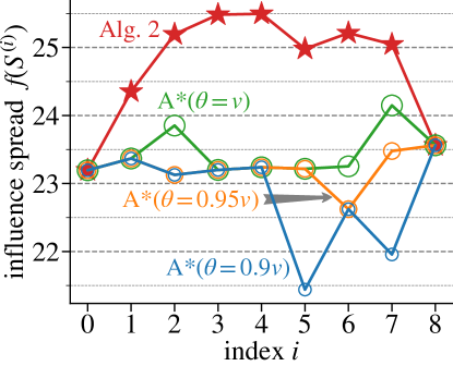
(a) karate network

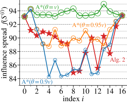
(b) physicians network

Figure 2. Influence spread of each set in the reconfiguration sequences returned by A* algorithm ($\theta=0.9v,0.95v,v$) and Algorithm 2, where $v=\min\{f(X),f(Y)\}$.

7.1.3. Results

We ran Algorithm 2 and the A* algorithm with $\theta=0.9v,0.95v,v$, where $v\triangleq\min\{f(X),f(Y)\}$, on karate and physicians. The obtained sequences were found to be all the shortest. Figure 2 displays the influence spread of sets in each reconfiguration sequence. On karate, the A* algorithm with $\theta=v$ and Algorithm 2 found an optimal reconfiguration sequence of value $v$. We can observe that the intermediate sets for Algorithm 2 were more influential than those for the A* algorithm. Figure 1 draws karate network, where each vertex is colored according to its probability of being activated by $X$, the fourth subset $S^{(4)}$ returned by Algorithm 2, or $Y$. We can see that many vertices are more likely to be activated by $S^{(4)}$ than by $X$ or $Y$, making it easy to transform from $X$ to $Y$. (See Appendix C for the entire reconfiguration sequence returned by Algorithm 2.) On physicians, Algorithm 2 found a reconfiguration sequence of value $84.9\approx 0.91v$, which is still drastically better than $\frac{1}{2}v$ envisioned from Theorem 5.1, though the A* algorithm’s sequence has value $v$. We finally report the number of oracle calls for an influence function: On karate, Algorithm 2 made $72$ calls and the A* algorithm made $1{,}428$ calls; on physicians, Algorithm 2 made $272$ calls and the A* algorithm made $53{,}987$ calls. (We stress that we do not report actual running time as it heavily depends on implementations of an unbiased estimator (Ohsaka, 2020) and scalability against large instances is beyond the scope of this paper.) In summary, Algorithm 2 produced a reconfiguration sequence of reasonable quality by making fewer oracle calls.

7.2. MAP Inference Reconfiguration

7.2.1. Problem Description

We formulate the reconfiguration of maximum a posteriori (MAP) inference on determinantal point process as USReco[tjar]. Determinantal point processes (DPPs) (Macchi, 1975; Borodin and Rains, 2005) are a probabilistic model on the power set $2^{[n]}$, which captures negative correlations among objects. Given a Gram matrix $\mathbf{\bm{A}}\in\mathbb{R}^{n\times n}$, a DPP defines the probability mass of each subset $S\subseteq[n]$ to be proportional to $\det(\mathbf{\bm{A}}_{S})$. Seeking a subset with the maximum determinant (i.e., $\max_{S\subseteq[n]}\det(\mathbf{\bm{A}}_{S})$), which is equivalent to MAP inference (Gillenwater et al., 2012), finds applications in recommendation and summarization (Wilhelm et al., 2018; Yao et al., 2016; Kulesza and Taskar, 2012). Since $\log\det(\mathbf{\bm{A}}_{S})$ as a set function in $S$ is submodular, the reconfiguration counterpart of MAP inference is USReco, whose motivation was explained in section 1.

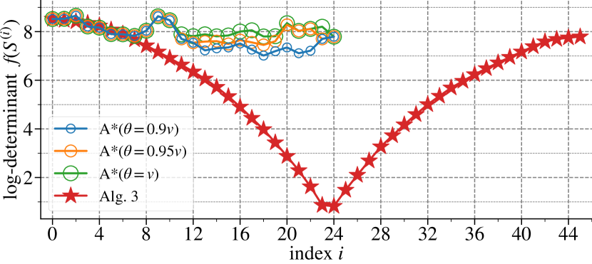
Figure 3. Log-determinant of each set in the reconfiguration sequences returned by A* algorithm ($\theta=0.9v,0.95v,v$) and Algorithm 3 on MovieLens 1M, where $v=\min\{f(X),f(Y)\}$.

7.2.2. Setup

We prepare a Gram matrix $\mathbf{\bm{A}}$ and a pair of input sets $X$ and $Y$. We used MovieLens 1M (Harper and Konstan, 2015), which consists of $1$ million ratings on $3{,}900$ movies from $6{,}040$ users of an online movie recommendation website MovieLens. We first selected $n=207$ movies with at least $1{,}000$ ratings and $m=839$ users who rated at least $100$ movies, resulting in an $n\times m$ movie-user rating matrix. We then ran Nonnegative Matrix Factorization (Boutsidis and Gallopoulos, 2008) with dimension $64$ to extract a feature vector $\mathbf{\bm{\phi}}_{i}\in\mathbb{R}^{64}$ with $\|\mathbf{\bm{\phi}}_{i}\|_{2}=1$ for each movie $i\in[n]$. The Gram matrix $\mathbf{\bm{A}}\in\mathbb{R}^{n\times n}$ is constructed as $A_{i,j}=\langle 2^{r_{i}-4}\mathbf{\bm{\phi}}_{i},2^{r_{j}-4}\mathbf{\bm{\phi}}_{j}\rangle$ for all $i,j\in[n]$, where $r_{i}$ is an average rating of movie $i$ between $[1,5]$. Since $\det(\mathbf{\bm{A}}_{S})$ is equal to $(\prod_{i\in S}2^{r_{i}-4})^{2}$ times the square volume of the parallelepiped spanned by $\{\mathbf{\bm{\phi}}_{i}\}_{i\in S}$ (Kulesza and Taskar, 2012), movies in a subset of large determinant are expected to be highly-rated and of diverse genres. An input submodular function $f$ is defined as $f(S)\triangleq\log\det(\mathbf{\bm{A}}_{S})$ for $S\subseteq[n]$. We created $X$ and $Y$ in a similar manner to the first experiment: We computed $X_{i}$ and $Y_{i}$ for $i\geq 1$ according to Eq. 4 until no further selection is possible and extracted those with the largest determinant, resulting is that $X\triangleq X_{24}$ and $Y\triangleq Y_{22}$, where $f(X)=8.52$ and $f(Y)=7.79$.

7.2.3. Results

We ran Algorithm 3 and the A* algorithm with $\theta=0.9v,0.95v,v$, where $v\triangleq\min\{f(X),f(Y)\}$. The A* algorithm produced reconfiguration sequences of length $24$ while Algorithm 3 produced a reconfiguration sequence of length $45$. Figure 3 plots the log-determinant of sets in each reconfiguration sequence. The A* algorithm with $\theta=v$ was able to find an optimal reconfiguration sequence $\mathcal{S}^{*}$. $22$ of the $24$ steps in $\mathcal{S}^{*}$ were found to be tj steps, which is quite different from the behavior of Algorithm 3. One possible reason is that log-determinant functions exhibit monotonicity when every eigenvalue of $\mathbf{\bm{A}}$ is greater than $1$ (Sharma et al., 2015); in fact, the principal submatrix of $\mathbf{\bm{A}}$ induced by $X$ and $Y$ has the minimum eigenvalue of $0.70$ and $0.76$, respectively, while the minimum eigenvalue of $\mathbf{\bm{A}}$ was approximately $0$. Hence, there is a sequence of tj steps that preserves the log-determinant large. As opposed to the success of Algorithm 2 for MSReco, Algorithm 3’s value was $0.823\approx 0.11v$, which is nine times smaller than the optimal value $v$. This result is easily expected from the mechanism of Algorithm 3, which includes singletons (i.e., $\{x_{1}\}$ and $\{y_{1}\}$) into the output sequence. The number of oracle calls for a log-determinant function was $553$ for Algorithm 3 and $105{,}412$ for the A* algorithm. We conclude that Algorithm 3 consumes fewer oracle calls but further development on approximation algorithms for MaxUSReco[tjar] is required.

8. Conclusion and Open Questions

We established an initial study on submodular reconfiguration problems, including intractability, (in)approximability, and numerical results. We conclude this paper with two open questions.

• Can we devise an approximation algorithm for MaxUSReco[tar]?

• Can the approximation factors in section 5 be made tight? We conjecture an $\mathcal{O}(1)$-factor approximability for MaxUSReco[tjar].

Appendix A Missing Proofs

Proof of Observation 4.1.

It is known (van den Heuvel, 2013) that a reachability problem defined in the reconfiguration framework is in NPSPACE if the following assumptions hold:

• given a possible solution, we can determine whether it is feasible in polynomial time;

• given two feasible solutions, we can decide if there is a reconfiguration step from one to the other in polynomial time.

It is easy to see that Problems 3.2, LABEL:, 3.3, LABEL: and 3.4 meet these assumptions. By Savitch’s theorem (Savitch, 1970), we have that PSPACE $=$ NPSPACE, which completes the proof. ∎

To prove PSPACE-hardness of Minimum Vertex Cover Reconfiguration (Lemma 4.4), we use a reduction from 3-SAT Reconfiguration (Gopalan et al., 2009). Given a 3-conjunctive normal form (3-CNF) formula $\phi$, of which each clause contains at most three literals (e.g., $\phi=(x_{1}\vee\overline{x_{2}}\vee x_{3})\wedge(x_{2}\vee\overline{x_{3}}\vee x_{4})\wedge(\overline{x_{1}}\vee x_{3}\vee\overline{x_{4}})$), 3-SAT asks to decide if there exists a truth assignment $\mathbf{\bm{\sigma}}$ for the variables of $\phi$ that satisfies all clauses of $\phi$ (e.g., $\mathbf{\bm{\sigma}}(x_{1})=\mathbf{\bm{\sigma}}(x_{2})=\textsf{True}$ and $\mathbf{\bm{\sigma}}(x_{3})=\mathbf{\bm{\sigma}}(x_{4})=\textsf{False}$). 3-SAT Reconfiguration is defined as:

Problem A.1 (3-SAT Reconfiguration (Gopalan et al., 2009)).

Given a 3-CNF formula $\phi$ and two satisfying truth assignments $\mathbf{\bm{\sigma}}^{x}$ and $\mathbf{\bm{\sigma}}^{y}$ of $\phi$, determine whether there exists a sequence of satisfying truth assignments of $\phi$ from $\mathbf{\bm{\sigma}}^{x}$ to $\mathbf{\bm{\sigma}}^{y}$, $\langle\mathbf{\bm{\sigma}}^{(0)}=\mathbf{\bm{\sigma}}^{x},\mathbf{\bm{\sigma}}^{(1)},\ldots,\mathbf{\bm{\sigma}}^{(\ell)}=\mathbf{\bm{\sigma}}^{y}\rangle$, such that each truth assignment is obtained from the previous one by a single variable flip; i.e., they differ in exactly one variable.

3-SAT is widely known to be NP-complete (Cook, 1971; Levin, 1973) while 3-SAT Reconfiguration is PSPACE-complete (Gopalan et al., 2009).

Proof of Lemma 4.4.

The proof mostly follows (Ito et al., 2011). We show a polynomial-time reduction from 3-SAT Reconfiguration. Suppose we are given a 3-CNF formula $\phi$ with $n$ variables $x_{1},\ldots,x_{n}$ and $m$ clauses $c_{1},\ldots,c_{m}$ and two satisfying truth assignments $\mathbf{\bm{\sigma}}^{x}$ and $\mathbf{\bm{\sigma}}^{y}$ of $\phi$. Starting with an empty graph, we construct a graph $G_{\phi}$ in polynomial time according to (Ito et al., 2011, Proof of Theorem 2):

• Step 1. for each variable $x_{i}$ in $\phi$, we add an edge to $G_{\phi}$, the endpoints of which are labeled $x_{i}$ and $\overline{x}_{i}$;

• Step 2. for each clause $c_{j}$ in $\phi$, we add a clique of size $|c_{j}|$ to $G_{\phi}$, each vertex in which corresponds to a literal in $c_{j}$;

• Step 3. we connect between two vertices in different components by an edge if they correspond to opposite literals of the same variable, e.g., $x_{i}$ and $\overline{x}_{i}$.

It is proven (Ito et al., 2011) that $G_{\phi}$ has a maximum independent set $I$ of size $m+n$ if and only if $\phi$ is satisfiable; here, $n$ vertices in $I$ are chosen from the endpoints of the $n$ edges corresponding to the variables of $\phi$, and $m$ vertices in $I$ are chosen from the $m$ cliques corresponding to the clauses of $\phi$. Using such $I$, we can uniquely construct a satisfying truth assignment $\mathbf{\bm{\sigma}}_{I}$ of $\phi$, which assigns True (resp. False) to $x_{i}$ if $I$ includes the endpoint labeled $x_{i}$ (resp. $\overline{x_{i}}$). On the other hand, for a fixed truth satisfying assignment $\mathbf{\bm{\sigma}}$, there may be exponentially many maximum independent sets $I$ such that $\mathbf{\bm{\sigma}}_{I}=\mathbf{\bm{\sigma}}$. Observe now the following facts for $G_{\phi}$ for which $\phi$ is satisfiable:

• For any two satisfying truth assignments $\mathbf{\bm{\sigma}}_{1}$ and $\mathbf{\bm{\sigma}}_{2}$ that differ in exactly one variable, there exist two maximum independent sets $I_{1}$ and $I_{2}$ such that $I_{1}$ is obtained from $I_{2}$ by a single tj step, $\mathbf{\bm{\sigma}}_{I_{1}}=\mathbf{\bm{\sigma}}_{1}$ and $\mathbf{\bm{\sigma}}_{I_{2}}=\mathbf{\bm{\sigma}}_{2}$.

• For any two maximum independent sets $I_{1}$ and $I_{2}$ corresponding to the same satisfying truth assignments (i.e., $\mathbf{\bm{\sigma}}_{I_{1}}=\mathbf{\bm{\sigma}}_{I_{2}}$), there exists a sequence of maximum independent sets corresponding to the same satisfying truth assignment from $I_{1}$ to $I_{2}$ under tj.

We now translate the above discussion into the language of vertex cover. Because a vertex set $C\subseteq V(G_{\phi})$ is a minimum vertex cover of $G_{\phi}$ if and only if $V(G_{\phi})\setminus C$ is a maximum independent set of $G_{\phi}$, $G_{\phi}$ has a minimum vertex cover $C$ of size $|V(G_{\phi})|-m-n$ if and only if $\phi$ is satisfiable; we can uniquely construct a satisfying truth assignment $\mathbf{\bm{\sigma}}_{V(G_{\phi})\setminus C}$. Consequently, for any two minimum vertex covers $C^{x}$ and $C^{y}$ of size $|V(G_{\phi})|-m-n$ such that $\mathbf{\bm{\sigma}}_{V(G_{\phi})\setminus C^{x}}=\mathbf{\bm{\sigma}}^{x}$ and $\mathbf{\bm{\sigma}}_{V(G_{\phi})\setminus C^{y}}=\mathbf{\bm{\sigma}}^{y}$, there exists a sequence of satisfying truth assignments from $\mathbf{\bm{\sigma}}^{x}$ to $\mathbf{\bm{\sigma}}^{y}$ that meets the specification for 3-SAT Reconfiguration if and only if there exists a sequence of minimum vertex covers from $C^{x}$ to $C^{y}$ under tj. Such vertex covers $C^{x}$ and $C^{y}$ can be found in polynomial time, which completes the reduction from 3-SAT Reconfiguration to MSReco. ∎

Proof of Theorem 4.6.

We demonstrate a polynomial-time reduction from Problem 4.3. Given a graph $G=(V,E)$ and two minimum vertex covers $C^{x}$ and $C^{y}$ of size $k$, we define a submodular function $f:2^{V}\to\mathbb{R}_{+}$ such that $f(S)$ is “the number of edges in $E$ that are incident to $S$ minus $\frac{1}{2}(n-|S|)$,” where $n\triangleq|V|$. Consider USReco[tjar] defined by $f$, $C^{x}$, $C^{y}$, and a threshold $\theta\triangleq|E|-\frac{k}{2}+\frac{n}{2}$. It turns out that any reconfiguration sequence from $C^{x}$ to $C^{y}$ does not include a vertex set of size either $k-1$ or $k+1$—that is, we can only apply tj steps—in the following case analysis on $f(S)$:

• if $|S|=k-1$ ($S$ cannot be a vertex cover): $f(S)\leq|E|-\frac{k}{2}+\frac{n}{2}-\frac{1}{2}$;

• if $|S|=k$ and $S$ is a vertex cover: $f(S)=|E|-\frac{k}{2}+\frac{n}{2}$;

• if $|S|=k$ and $S$ is not a vertex cover: $f(S)\leq|E|-\frac{k}{2}+\frac{n}{2}-1$;

• if $|S|=k+1$ ($S$ may be a vertex cover): $f(S)\leq|E|-\frac{k}{2}+\frac{n}{2}-\frac{1}{2}$.

Therefore, a reconfiguration sequence on the Minimum Vertex Cover Reconfiguration instance is a reconfiguration sequence on the USReco[tjar] instance, and vice versa, which completes the reduction; the PSPACE-hardness follows from Lemma 4.4. ∎

Proof for $(1-\kappa)^{2}$-approximation in Theorem 5.1.

We reuse the notations $R,X^{\prime},Y^{\prime},k^{\prime},x_{i},y_{i},X_{i},Y_{i}$ from the proof of Theorem 5.1 in the main body. We denote by $\kappa$ the total curvature of $f$; note that the residual $f_{R}$ has a total curvature not more than $\kappa$.

Showing that $f(\mathcal{S})\geq(1-\kappa)^{2}\min\{f(X),f(Y)\}$ is sufficient. For each $i\in[k^{\prime}]$, we denote $\Delta x_{i}\triangleq f_{R}(X_{i})-f_{R}(X_{i-1})$ and $\Delta y_{i}\triangleq f_{R}(Y_{i})-f_{R}(Y_{i-1})$. Note that $\Delta x_{i}$ and $\Delta y_{i}$ are monotonically nonincreasing in $i$ due to Eq. 1; i.e., $\Delta x_{1}\geq\Delta x_{2}\geq\cdots\geq\Delta x_{k^{\prime}}$ and $\Delta y_{1}\geq\Delta y_{2}\geq\cdots\geq\Delta y_{k^{\prime}}$. We define a set function $\overline{f_{R}}:2^{[n]\setminus R}\to\mathbb{R}_{+}$ such that, for each $S\subseteq[n]\setminus R$, $\overline{f_{R}}(S)\triangleq\sum_{e\in S}f_{R}(\{e\}).$ Note that $\overline{f_{R}}$ is a monotone modular function, and that $\overline{f_{R}}(S)$ gives an upper bound of $f_{R}(S)$. Moreover, $\overline{f_{R}}$ gives a $(1-\kappa)$-factor approximation to $f_{R}$ (e.g., (Iyer et al., 2013, Lemma 2.1)); i.e.,

(6) $$(1-\kappa)\overline{f_{R}}(S)\leq f_{R}(S)\leq\overline{f_{R}}(S),\text{ for all }S\subseteq[n]\setminus R.$$

We will bound $\overline{f_{R}}(X_{k^{\prime}-i}\uplus Y_{i})$ from below for each $i\in[k^{\prime}-1]$ in a case analysis. We have two cases to consider:

• $\Delta y_{i}\geq\Delta x_{k^{\prime}-i+1}$. We then have that $\Delta y_{1}+\cdots+\Delta y_{i}\geq\Delta x_{k^{\prime}-i+1}+\cdots+\Delta x_{k}$. By adding $\sum_{1\leq j\leq k^{\prime}-i}\Delta x_{j}$ to both sides, we obtain that

  $$\sum_{1\leq j\leq i}\Delta y_{j}+\sum_{1\leq j\leq k^{\prime}-i}\Delta x_{j} \geq\sum_{k^{\prime}-i+1\leq j\leq k^{\prime}}\Delta x_{j}+\sum_{1\leq j\leq k^{\prime}-i}\Delta x_{j}$$

  $$\Rightarrow f_{R}(Y_{i})+f_{R}(X_{k^{\prime}-i}) \geq f_{R}(X_{k^{\prime}})+f_{R}(\emptyset).$$

  Simple calculation using Eq. 6 yields that $\overline{f_{R}}(Y_{i}\uplus X_{k^{\prime}-i})=\overline{f_{R}}(Y_{i})+\overline{f_{R}}(X_{k^{\prime}-i})\geq(1-\kappa)\overline{f_{R}}(X^{\prime}),$ where we note that $\overline{f_{R}}(\emptyset)=0$.

• $\Delta y_{i}\leq\Delta x_{k^{\prime}-i+1}$. We then have that $\Delta x_{1}+\cdots+\Delta x_{k^{\prime}-i}\geq\Delta y_{i+1}+\cdots+\Delta y_{k^{\prime}}$. By adding $\sum_{1\leq j\leq i}\Delta y_{j}$ to both sides and using Eq. 6, we obtain the following: $\overline{f_{R}}(Y_{i}\uplus X_{k^{\prime}-i})=\overline{f_{R}}(Y_{i})+\overline{f_{R}}(X_{k^{\prime}-i})\geq(1-\kappa)\overline{f_{R}}(Y^{\prime}).$

We thus have that, in either case,

(7) $$\overline{f_{R}}(X_{k^{\prime}-i}\uplus Y_{i})\geq(1-\kappa)\min\{\overline{f_{R}}(X^{\prime}),\overline{f_{R}}(Y^{\prime})\}.$$

Observing that Eq. 7 is true even if $i=0,k^{\prime}$, we bound the value $f(\mathcal{S})$ of the resulting reconfiguration sequence $\mathcal{S}$ as follows:

$$f(\mathcal{S}) =\min_{0\leq i\leq k^{\prime}}f_{R}(X_{k^{\prime}-i}\uplus Y_{i})+f(R)$$

$$\geq\min_{0\leq i\leq k^{\prime}}(1-\kappa)\overline{f_{R}}(X_{k^{\prime}-i}\uplus Y_{i})+f(R)$$

$$\geq(1-\kappa)^{2}\min\{\overline{f_{R}}(X^{\prime}),\overline{f_{R}}(Y^{\prime})\}+f(R)$$

$$\geq(1-\kappa)^{2}\min\{f(X),f(Y)\}.\qed$$

Proof of Observation 5.2.

We explicitly construct such an instance that meets the specification. Define $n\triangleq 5$, $\Sigma\triangleq\{a,b,c,d\}$, $V_{1}=\{a,b\}$, $V_{2}=\{c,d\}$, $V_{3}=\{a,c\}$, $V_{4}=\{b,d\}$, and $V_{5}=\Sigma$. We then define a coverage function $f:2^{[n]}\to\mathbb{R}_{+}$ such that $f(S)\triangleq\frac{|\bigcup_{i\in S}V_{i}|}{|\Sigma|}$ for $S\subseteq[n]$. Consider MaxMSReco defined by $f$, $X\triangleq\{1,2\}$, and $Y\triangleq\{3,4\}$. An optimal reconfiguration sequence from $X$ to $Y$ is $\mathcal{S}^{*}=\langle\{1,2\},\{1,5\},\{3,5\},\{3,4\}\rangle$, whose value is $f(\mathcal{S}^{*})=1$. On the other hand, when we are restricted to have subsets of $X\cup Y=\{1,2,3,4\}$ in the output sequence, we must touch either of $\{1,3\},\{1,4\},\{2,3\},\{2,4\}$, whose function value is $\frac{3}{4}$. ∎

Proof of Observation 5.4.

We construct such an instance that meets the specification. Suppose $n$ is a positive integer divisible by $4$. Define an edge-weighted graph $G=([n],E)$, where $E\triangleq\{(i,\frac{n}{2}+i)\mid i\in[\frac{n}{2}]\}$, and the weight of edge $(i,\frac{n}{2}+i)$ is $i^{-1}$. Let $f:2^{[n]}\to\mathbb{R}_{+}$ be a weighted cut function defined by $G$. Consider MaxUSReco[tjar] defined by $f$, $X\triangleq[\frac{n}{2}]$, and $Y\triangleq[n]\setminus S$. Algorithm 3 produces a reconfiguration sequence of value $1$. On the other hand, Algorithm 2 returns a reconfiguration sequence includes $\{1,\ldots,\frac{n}{4}\}\uplus\{\frac{n}{2}+1,\ldots,\frac{n}{2}+\frac{n}{4}\}$, whose cut value is $0$. ∎

Proof of Observation 5.5.

We construct such an instance that meets the specification. We define a submodular set function $f:2^{[2]}\to\mathbb{R}_{+}$ as $f(\emptyset)=f(\{1,2\})=0$ and $f(\{1\})=f(\{2\})=1$. Consider MaxUSReco[tar] defined by $f$, $X\triangleq\{1\}$, and $Y\triangleq\{2\}$. Since we can use tar steps only, any reconfiguration sequence $\mathcal{S}$ from $X$ to $Y$ (including the optimal one) must pass through at least either one of $\emptyset$ or $\{1,2\}$; thus, $f(\mathcal{S})$ must be $0$. ∎

Proof of Theorem 6.1.

We show that to solve Minimum Vertex Cover Reconfiguration exactly, a $(1-\frac{1+\epsilon}{n^{2}})$-approximation algorithm for MaxMSReco is sufficient. Recall that given a graph $G=(V,E)$ and two minimum vertex covers $C^{x}$ and $C^{y}$, the polynomial-time reduction introduced in the proof of Theorem 4.2 constructs an instance $f,C^{x},C^{y}$ of MaxMSReco, for which an optimal reconfiguration sequence $\mathcal{S}^{*}$ satisfies that $f(\mathcal{S}^{*})=|E|$ if the answer to the Minimum Vertex Cover Reconfiguration instance is “yes” and $f(\mathcal{S}^{*})\leq|E|-1$ otherwise. To distinguish the two cases, it is sufficient to approximate the optimal value of MaxMSReco within a factor of $\frac{|E|-1+\epsilon}{|E|}\leq 1-\frac{1+\epsilon}{n^{2}}$ for any $\epsilon>0$, completing the proof. ∎

Proof of Theorem 6.3.

The proof is almost the same as that of Theorem 6.2. We only need to claim that for any $S\subseteq[n]$, we can construct a reconfiguration sequence $\mathcal{S}$ whose value is $g(\mathcal{S})=\Upsilon+f(S)$ using only tar steps: an example of such a sequence is $\langle X,\cdots$ adding elements of $S$ one by one $\cdots,X\cup S,\{x_{1}\}\cup S,\{x_{1},y_{1}\}\cup S,\{y_{1}\}\cup S,Y\cup S,\cdots$ removing elements of $S$ one by one $\cdots,Y\rangle$. ∎

Appendix B A* Search Algorithm

Algorithm 4 describes an A* search algorithm for MSReco and USReco. In A* algorithms (Hart et al., 1968), we have a table $g$ for storing the minimum number of reconfiguration steps required to transform from $X$ to each set $S$, and a heuristic function $h:2^{[n]}\to\mathbb{R}$ for underestimating the number of reconfiguration steps required to transform from each set $S$ to $Y$. For example, $h(S)=\frac{|S\setminus Y|+|Y\setminus S|}{2}$ under tj and $h(S)=\max(|S\setminus Y|,|Y\setminus S|)$ under tjar, which are both admissible and consistent (Pearl, 1984). We continue the iterations, which pop a set $S$ with minimum $g[S]+h(S)$ and explore each of the adjacent feasible sets $T$, until we found $T=Y$ or no further expansion is possible. Since two or more tie sets may have the same score, we used a Last-In-First-Out policy (Asai and Fukunaga, 2016). Note that Algorithm 4 may require exponential time in the worst case.

Algorithm 4 A* algorithm for MSReco and USReco.

1:submodular function $f:2^{[n]}\to\mathbb{R}_{+}$, two sets $X,Y$, threshold $\theta$, heuristic function $h:2^{[n]}\to\mathbb{R}_{+}$.

2:initialize priority queue $\mathtt{OPEN}$, and $\mathtt{CLOSE}\leftarrow\emptyset$.

3:declare empty hash table $g$, and push $X$ with score $h(X)$ into $\mathtt{OPEN}$.

4:while $\mathtt{OPEN}$ is not empty do

5:    pop set $S$ with minimum score from $\mathtt{OPEN}$ and push $S$ into $\mathtt{CLOSE}$.

6:    if $S=Y$ then: return reconfiguration sequence constructed using $\pi$.

7:    for all set $T$ adjacent to $S$ such that $f(T)\geq\theta$ do

8:        if $T\in\mathtt{OPEN}$ and $g[S]+1<g[T]$ then $\triangleright$ reinsert node.

9:           $g[T]\leftarrow g[S]+1$ and $\pi[T]\leftarrow S$.

10:           remove $T$ from $\mathtt{OPEN}$ and push $T$ with score $g[T]+h(T)$ into $\mathtt{OPEN}$.

11:        else if $T\in\mathtt{CLOSE}$ and $g[S]+1<g[T]$ then $\triangleright$ reopen node.

12:           $g[T]\leftarrow g[S]+1$ and $\pi[T]\leftarrow S$.

13:           remove $T$ from $\mathtt{CLOSE}$ and push $T$ with score $g[T]+h(T)$ into $\mathtt{OPEN}$.

14:        else if $T\not\in\mathtt{OPEN}$ and $T\not\in\mathtt{CLOSE}$ then $\triangleright$ open node.

15:           $g[T]\leftarrow g[S]+1$ and $\pi[T]\leftarrow S$.

16:           push $T$ with score $g[T]+h(T)$ into $\mathtt{OPEN}$.             

Appendix C Additional Result

Table 2. Sequence returned by Algorithm 2 on karate.

index $i$	seed set $S^{(i)}$	influence $f(S^{(i)})$
0	$\{34,2,7,32,4,11,30,9\}$	23.2
1	$\{34,2,7,32,4,11,30,1\}$	24.3
2	$\{34,2,7,32,4,11,33,1\}$	25.2
3	$\{34,2,7,32,4,3,33,1\}$	25.5
4	$\{34,2,7,32,6,3,33,1\}$	25.5
5	$\{34,2,7,14,6,3,33,1\}$	25.0
6	$\{34,2,24,14,6,3,33,1\}$	25.2
7	$\{34,25,24,14,6,3,33,1\}$	25.0
8	$\{27,25,24,14,6,3,33,1\}$	23.6

References

- (1)
- Adomavicius and Zhang (2012) Gediminas Adomavicius and Jingjing Zhang. 2012. Stability of recommendation algorithms. ACM Trans. Inf. Syst. 30, 4 (2012), 23:1–23:31.
- Arora et al. (2017) Akhil Arora, Sainyam Galhotra, and Sayan Ranu. 2017. Debunking the Myths of Influence Maximization: An In-Depth Benchmarking Study. In SIGMOD. 651–666.
- Arora and Barak (2009) Sanjeev Arora and Boaz Barak. 2009. Computational Complexity: A Modern Approach. Cambridge University Press.
- Asai and Fukunaga (2016) Masataro Asai and Alex Fukunaga. 2016. Tiebreaking strategies for A* search: How to explore the final frontier. In AAAI. 673–679.
- Bonsma and Cereceda (2009) Paul Bonsma and Luis Cereceda. 2009. Finding paths between graph colourings: PSPACE-completeness and superpolynomial distances. Theor. Comput. Sci. 410, 50 (2009), 5215–5226.
- Borgs et al. (2014) Christian Borgs, Michael Brautbar, Jennifer Chayes, and Brendan Lucier. 2014. Maximizing Social Influence in Nearly Optimal Time. In SODA. 946–957.
- Borodin and Rains (2005) Alexei Borodin and Eric M. Rains. 2005. Eynard-Mehta theorem, Schur process, and their Pfaffian analogs. J. Stat. Phys. 121, 3–4 (2005), 291–317.
- Boutsidis and Gallopoulos (2008) Christos Boutsidis and Efstratios Gallopoulos. 2008. SVD based initialization: A head start for nonnegative matrix factorization. Pattern Recognit. 41, 4 (2008), 1350–1362.
- Buchbinder and Feldman (2018a) Niv Buchbinder and Moran Feldman. 2018a. Deterministic algorithms for submodular maximization problems. ACM Trans. Algorithms 14, 3 (2018), 1–20.
- Buchbinder and Feldman (2018b) Niv Buchbinder and Moran Feldman. 2018b. Submodular Functions Maximization Problems. In Handbook of Approximation Algorithms and Metaheuristics. Chapman and Hall/CRC, 771–806.
- Buchbinder et al. (2015) Niv Buchbinder, Moran Feldman, Joseph Seffi, and Roy Schwartz. 2015. A tight linear time (1/2)-approximation for unconstrained submodular maximization. SIAM J. Comput. 44, 5 (2015), 1384–1402.
- Cardinal et al. (2020) Jean Cardinal, Erik D. Demaine, David Eppstein, Robert A. Hearn, and Andrew Winslow. 2020. Reconfiguration of satisfying assignments and subset sums: Easy to find, hard to connect. Theor. Comput. Sci. 806 (2020), 332–343.
- Chen et al. (2018) Laming Chen, Guoxin Zhang, and Eric Zhou. 2018. Fast greedy MAP inference for determinantal point process to improve recommendation diversity. In NeurIPS. 5622–5633.
- Chen et al. (2010) Wei Chen, Chi Wang, and Yajun Wang. 2010. Scalable Influence Maximization for Prevalent Viral Marketing in Large-Scale Social Networks. In KDD. 1029–1038.
- Conforti and Cornuéjols (1984) Michele Conforti and Gérard Cornuéjols. 1984. Submodular set functions, matroids and the greedy algorithm: Tight worst-case bounds and some generalizations of the Rado-Edmonds theorem. Discrete Appl. Math. 7, 3 (1984), 251–274.
- Cook (1971) Stephen A. Cook. 1971. The complexity of theorem-proving procedures. In STOC. 151–158.
- Domingos and Richardson (2001) Pedro Domingos and Matt Richardson. 2001. Mining the Network Value of Customers. In KDD. 57–66.
- Feige (1998) Uriel Feige. 1998. A threshold of ln for approximating set cover. J. ACM 45, 4 (1998), 634–652.
- Feige et al. (2011) Uriel Feige, Vahab S. Mirrokni, and Jan Vondrák. 2011. Maximizing non-monotone submodular functions. SIAM J. Comput. 40, 4 (2011), 1133–1153.
- Garey and Johnson (1979) Michael R. Garey and David S. Johnson. 1979. Computers and Intractability: A Guide to the Theory of NP-Completeness. W. H. Freeman.
- Gillenwater et al. (2012) Jennifer Gillenwater, Alex Kulesza, and Ben Taskar. 2012. Near-optimal MAP inference for determinantal point processes. In NIPS. 2735–2743.
- Goldenberg et al. (2001) Jacob Goldenberg, Barak Libai, and Eitan Muller. 2001. Talk of the network: A complex systems look at the underlying process of word-of-mouth. Mark. Lett. 12, 3 (2001), 211–223.
- Gopalan et al. (2009) Parikshit Gopalan, Phokion G. Kolaitis, Elitza Maneva, and Christos H. Papadimitriou. 2009. The connectivity of Boolean satisfiability: computational and structural dichotomies. SIAM J. Comput. 38, 6 (2009), 2330–2355.
- Harper and Konstan (2015) F. Maxwell Harper and Joseph A. Konstan. 2015. The MovieLens datasets: History and context. ACM Trans. Interact. Intell. Syst. 5, 4 (2015), 1–19.
- Hart et al. (1968) Peter E. Hart, Nils J. Nilsson, and Bertram Raphael. 1968. A formal basis for the heuristic determination of minimum cost paths. IEEE Trans. Syst. Sci. Cybern. 4, 2 (1968), 100–107.
- Hearn and Demaine (2005) Robert A. Hearn and Erik D. Demaine. 2005. PSPACE-Completeness of Sliding-Block Puzzles and Other Problems through the Nondeterministic Constraint Logic Model of Computation. Theor. Comput. Sci. 343, 1-2 (2005), 72–96.
- Ito and Demaine (2014) Takehiro Ito and Erik D. Demaine. 2014. Approximability of the subset sum reconfiguration problem. J. Comb. Optim. 28, 3 (2014), 639–654.
- Ito et al. (2011) Takehiro Ito, Erik D. Demaine, Nicholas J.A. Harvey, Christos H. Papadimitriou, Martha Sideri, Ryuhei Uehara, and Yushi Uno. 2011. On the complexity of reconfiguration problems. Theor. Comput. Sci. 412, 12-14 (2011), 1054–1065.
- Ito et al. (2016) Takehiro Ito, Hiroyuki Nooka, and Xiao Zhou. 2016. Reconfiguration of vertex covers in a graph. IEICE Trans. Inf. & Syst. 99, 3 (2016), 598–606.
- Iyer et al. (2013) Rishabh K. Iyer, Stefanie Jegelka, and Jeff A. Bilmes. 2013. Curvature and optimal algorithms for learning and minimizing submodular functions. In NIPS. 2742–2750.
- Johnson et al. (2016) Matthew Johnson, Dieter Kratsch, Stefan Kratsch, Viresh Patel, and Daniël Paulusma. 2016. Finding shortest paths between graph colourings. Algorithmica 75, 2 (2016), 295–321.
- Johnson and Story (1879) Wm Woolsey Johnson and William Edward Story. 1879. Notes on the “15” puzzle. Am. J. Math. 2, 4 (1879), 397–404.
- Kamiński et al. (2012) Marcin Kamiński, Paul Medvedev, and Martin Milanič. 2012. Complexity of independent set reconfigurability problems. Theor. Comput. Sci. 439 (2012), 9–15.
- Karp (1972) Richard M. Karp. 1972. Reducibility among combinatorial problems. In Complexity of Computer Computations. 85–103.
- Kempe et al. (2003) David Kempe, Jon Kleinberg, and Éva Tardos. 2003. Maximizing the Spread of Influence through a Social Network. In KDD. 137–146.
- Krause and Golovin (2014) Andreas Krause and Daniel Golovin. 2014. Submodular Function Maximization. In Tractability: Practical Approaches to Hard Problems. 71–104.
- Krause et al. (2008) Andreas Krause, Ajit Paul Singh, and Carlos Guestrin. 2008. Near-optimal sensor placements in Gaussian processes: Theory, efficient algorithms and empirical studies. J. Mach. Learn. Res. 9 (2008), 235–284.
- Kulesza and Taskar (2012) Alex Kulesza and Ben Taskar. 2012. Determinantal Point Processes for Machine Learning. Found. Trends Mach. Learn. 5, 2–3 (2012), 123–286.
- Kunegis (2013) Jérôme Kunegis. 2013. KONECT – The Koblenz Network Collection. In WWW Companion. 1343–1350.
- Leskovec et al. (2007a) Jure Leskovec, Jon Kleinberg, and Christos Faloutsos. 2007a. Graph Evolution: Densification and Shrinking Diameters. ACM Trans. Knowl. Discov. Data 1, 1 (2007), 2.
- Leskovec et al. (2007b) Jure Leskovec, Andreas Krause, Carlos Guestrin, Christos Faloutsos, Jeanne VanBriesen, and Natalie Glance. 2007b. Cost-effective Outbreak Detection in Networks. In KDD. 420–429.
- Levin (1973) Leonid Anatolevich Levin. 1973. Universal sequential search problems. Probl. Peredachi Inf. 9, 3 (1973), 115–116.
- Lichtenstein and Sipser (1980) David Lichtenstein and Michael Sipser. 1980. Go is polynomial-space hard. J. ACM 27, 2 (1980), 393–401.
- Lin and Bilmes (2011) Hui Lin and Jeff Bilmes. 2011. A class of submodular functions for document summarization. In ACL-HLT. 510–520.
- Loukides et al. (2020) Grigorios Loukides, Robert Gwadera, and Shing-Wan Chang. 2020. Overexposure-aware influence maximization. ACM Trans. Internet Technol. 20, 4 (2020), 1–31.
- Lovász (1983) László Lovász. 1983. Submodular Functions and Convexity. In Mathematical Programming – The State of the Art. 235–257.
- Macchi (1975) Odile Macchi. 1975. The coincidence approach to stochastic point processes. Adv. Appl. Probab. 7, 1 (1975), 83–122.
- Mirzasoleiman et al. (2016) Baharan Mirzasoleiman, Ashwinkumar Badanidiyuru, and Amin Karbasi. 2016. Fast constrained submodular maximization: Personalized data summarization. In ICML. 1358–1367.
- Mouawad (2015) Amer Mouawad. 2015. On Reconfiguration Problems: Structure and Tractability. Ph. D. Dissertation. University of Waterloo.
- Nemhauser and Wolsey (1978) George L. Nemhauser and Laurence A. Wolsey. 1978. Best algorithms for approximating the maximum of a submodular set function. Math. Oper. Res. 3, 3 (1978), 177–188.
- Nemhauser et al. (1978) George L. Nemhauser, Laurence A. Wolsey, and Marshall L. Fisher. 1978. An analysis of the approximations for maximizing submodular set functions. Math. Program. 14 (1978), 265–294.
- Nishimura (2018) Naomi Nishimura. 2018. Introduction to Reconfiguration. Algorithms 11, 4 (2018), 52.
- Ohsaka (2020) Naoto Ohsaka. 2020. The solution distribution of influence maximization: A high-level experimental study on three algorithmic approaches. In SIGMOD.
- Ohsaka et al. (2016) Naoto Ohsaka, Takuya Akiba, Yuichi Yoshida, and Ken-ichi Kawarabayashi. 2016. Dynamic Influence Analysis in Evolving Networks. Proc. VLDB Endow. 9, 12 (2016), 1077–1088.
- Pearl (1984) Judea Pearl. 1984. Heuristics: Intelligent Search Strategies for Computer Problem Solving. (1984).
- Savitch (1970) Walter J. Savitch. 1970. Relationships between nondeterministic and deterministic tape complexities. J. Comput. Syst. Sci. 4, 2 (1970), 177–192.
- Schrijver (2003) Alexander Schrijver. 2003. Combinatorial Optimization: Polyhedra and Efficiency. Springer Science & Business Media.
- Sharma et al. (2015) Dravyansh Sharma, Ashish Kapoor, and Amit Deshpande. 2015. On greedy maximization of entropy. In ICML. 1330–1338.
- Tang et al. (2014) Youze Tang, Xiaokui Xiao, and Yanchen Shi. 2014. Influence Maximization: Near-Optimal Time Complexity Meets Practical Efficiency. In SIGMOD. 75–86.
- van den Heuvel (2013) Jan van den Heuvel. 2013. The complexity of change. In Surveys in Combinatorics 2013. Vol. 409. 127–160.
- Vargas and Castells (2011) Saúl Vargas and Pablo Castells. 2011. Rank and relevance in novelty and diversity metrics for recommender systems. In RecSys. 109–116.
- Vondrák (2010) Jan Vondrák. 2010. Submodularity and Curvature: The Optimal Algorithm (Combinatorial Optimization and Discrete Algorithms). RIMS Kôkyûroku Bessatsu 23 (2010), 253–266.
- Wilhelm et al. (2018) Mark Wilhelm, Ajith Ramanathan, Alexander Bonomo, Sagar Jain, Ed H. Chi, and Jennifer Gillenwater. 2018. Practical diversified recommendations on YouTube with determinantal point processes. In CIKM. 2165–2173.
- Yao et al. (2016) Jin-ge Yao, Feifan Fan, Wayne Xin Zhao, Xiaojun Wan, Edward Y. Chang, and Jianguo Xiao. 2016. Tweet Timeline Generation with Determinantal Point Processes. In AAAI. 3080–3086.