Seeing behind black hole horizons in SYK

Abstract

We present an explicit reconstruction of the interior of an AdS₂ black hole in Jackiw-Teitelboim gravity, that is entirely formulated in the dual SYK model and makes no direct reference to the gravitational bulk. We do this by introducing a probe “observer” in the right wormhole exterior and using the prescription of [arXiv:2009.04476] to transport SYK operators along the probe’s infalling worldline and into the black hole interior, using an appropriate SYK modular Hamiltonian. Our SYK computation recovers the precise proper time at which signals sent from the left boundary are registered by our observer’s apparatus inside the wormhole. The success of the computation relies on the universal properties of SYK and we outline a promising avenue for extending it to higher dimensions and applying it to the computation of scattering amplitudes behind the horizon.

1 Introduction and summary

In this work, we perform an explicit computation demonstrating the ability of the recent proposal Jafferis:2020ora to holographically reconstruct operators behind black hole horizons, while relying entirely on boundary data.

The framework of Jafferis:2020ora outlines an intrinsically holographic method for transporting local operators along the trajectory of a selected bulk “observer” or probe, which propagates in some ambient geometry. The central idea is that upon tracing out the probe’s internal degrees of freedom, the rest of the Universe, which we call the system, is endowed with a reduced density matrix, $\rho$, as a consequence of its initial entanglement with the probe. The key observation was that, in certain states, the unitary flow $\rho^{is}$, called modular flow, propagates bulk operators, initially localized near the probe, along the probe’s worldline by translating them in proper time by an amount equal to

$$\tau_{proper}=\frac{\beta_{probe}}{2\pi}\,s$$ (1)

while keeping their location relative to the worldline fixed. The parameter $\beta_{probe}$ is an effective inverse temperature associated with the probe’s mixed state which we will make precise in the main text.

Practically, the introduction of the observer is achieved by entangling our holographic system with an external reference, representing the observer’s internal degrees of freedom; the system’s modular flow $\rho^{is}$ is then obtained by tracing out that reference. The reader is encouraged to consult Jafferis:2020ora for an in-depth exposition to the method and the arguments for it. The modular time/proper time correspondence, in the form stated here, has a limited regime of validity but it becomes the seed for a general holographic construction of an observer’s local proper time Hamiltonian, which is explained in an upcoming paper LamprouJafferisdeBoer . The most exciting possibility created by this proposal is obtaining holographic access to the local operators in the interior of black holes, by propagating bulk fields in the exterior with the modular flow of an infalling probe for the appropriate (finite) amount of modular time (Fig. 1c).

In this paper, we explicitly apply this method, within its expected regime of validity, in order to test this interior reconstruction. The setup of our computation is the $AdS_{2}$/SYK correspondence Sachdev:2010um , where an eternal $AdS_{2}$ wormhole solution of Jackiw-Teitelboim gravity is described microscopically by a pair of dynamically decoupled SYK systems (which we call SYK_l and SYK_r) in the thermofield double state. Each SYK model sachdev1993gapless ; kitaev2015simple is a quantum mechanical system that consists of $N$ Majorana fermions $\psi_{l,r}^{j}$ and has a $q$-local Hamiltonian with random couplings drawn from a Gaussian ensemble maldacena2016remarks . The infalling probe we wish to co-move with is a configuration of Majorana fermions introduced near the right asymptotic boundary, entangled with an external reference system of Dirac fermions. The probe is introduced by inserting in the Euclidean path integral that prepares the thermofield double state dual to the empty wormhole (Fig. 1a), an operator $U_{sys+ref}$ that entangles our system with the reference.

Following the proposal of Jafferis:2020ora , we proceed by analyzing, directly in the pair of SYK models, the evolution of a fermion $\psi_{r}$ of SYK_r with the unitary $\rho^{is}$, where $\rho$ is the reduced density matrix of SYK${}_{l}\times$SYK_r after tracing out the reference. To test the success of our reconstruction beyond the horizon, we study the causal influence of an excitation $\psi_{l}(t)$ inserted in the left asymptotic boundary at time $t$, on the modular flow of the right exterior operator $\rho^{-is}\psi_{r}\rho^{is}$, as a function of modular time $s$, by evaluating the anticommutator:

$$W(s,t)=\text{Tr}\left(\rho\{\rho^{-is}\psi_{r}\rho^{is},\psi_{l}(t)\}\right)$$ (2)

The bulk expectation for $W$ is the following: When the backreaction of the probe is small, the semiclassical geometry of the wormhole implies that the causal propagator $W$ vanishes for the range of proper times the flowed operator remains spacelike separated from the left insertion, and transitions to an $O(1)$ value at timelike separations, with a sharp spike occurring at the proper time when the former crosses the bulk lightcone of the latter.

Our SYK computation exactly reproduces this expected bulk propagator together with the precise proper time of lightcone crossing, in the large $q,N$ and low temperature limit, after the determination of the conversion factor $\beta_{probe}$ in (1). Our results, therefore, establish that the method proposed in Jafferis:2020ora constitutes a practically useful tool for the holographic reconstruction of black hole interior operators.

Summary of our results

We setup the SYK computation in Section 2. We first prepare the SYK state dual to an AdS wormhole that contains a probe entangled with a reference, in Section 2.1 and 2.2. We devote Section 2.3 to the detailed discussion of the bulk trajectory followed by this infalling probe and the behavior of the bulk-to-boundary causal propagator as a function of the probe’s proper time —the object we aim to compute holographically. In order to perform the dual SYK computation of $W$ and test its agreement with this bulk expectation, we introduce a replica trick, explained in Section 2.4, which translates the computation of $W$ to the evaluation of the SYK propagator on the Euclidean “necklace” diagram shown in Fig. 2a. In the rest of the paper, we present this computation from two different perspectives, using the microscopic SYK dynamics (Section 3) and the bulk JT path integral (Section 4), in an attempt to clarify the physics that underlies its success.

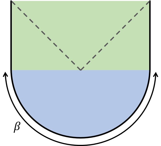
(a)

(b)

   

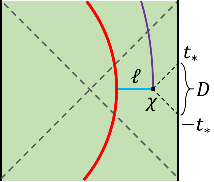
(c)

Figure 1: (a) Euclidean path integral preparation of the thermofield double state. The blue half disk is Euclidean path integral and the green strip is the Lorentzian continuation. (b) Euclidean path integral preparation of the thermofield double state with a probe following geodesic (25), which is plotted as the red curve. The purple curve is the Euclidean geodesic of the probe. (c) HKLL reconstruction of a bulk spinor field $\chi$ (black dot) with $\ell$ distance from the probe (red curve). Its boundary representation involves an integral of the HKLL kernel over the boundary region $D(t_{*})=[-t_{*},t_{*}]$ which is spacelike separated from $\chi$. Translating the bulk field $\chi$, originally located outside the horizon, along the proper time of the red geodesic, while keeping its geodesic distance from this geodesic fixed (purple curve), allows us to probe the $AdS_{2}$ wormhole interior. In the dual SYK model, this proper time translation is generated by the modular flow $\rho^{is}$ of the red probe, after tracing out the reference system it is entangled with.

In order to pave the way for the subsequent technical analysis, Section 2.4 offers some intuition for the behavior of the replica correlator in the limits of very large and very small probe entropy $S_{probe}$, showing that both lead to a trivial anticommutator $W(s,t)\rightarrow 0$, for all $s$, albeit for different reasons, and highlighting the importance of the intermediate $S_{probe}$ regime for getting interesting physics. In particular, $S_{probe}$ serves as an order parameter for the different phases of the dual Euclidean gravity path integral with the “necklace” diagram boundary conditions (Fig. 2a). At $S_{probe}\sim O(N)$ the dominant replica saddle consists of two disconnected disks associated with the left and right SYK boundary conditions, respectively —a factorization that yields a modular flow that does not mix SYK_l and SYK_r hence $W(s,t)\rightarrow 0$, for all $s$. The bulk interpretation of this behavior comes from the large backreaction of our probe which elongates the ambient wormhole and destroys the shared interior region, rendering the infalling observer incapable of receiving causal signals from the other side. As we decrease $S_{probe}$, a new dominant JT saddle appears describing a Euclidean wormhole with cylindrical topology (Fig. 2c) which, however, degenerates again as we take the limit $S_{probe}\to 0$ (Fig. 2d). It is precisely this Euclidean wormhole phase in the intermediate $S_{probe}$ regime that generates an interesting anticommutator $W$ which reflects the reception of signals sent from the left exterior by the observer falling in from the right. The critical point of this phase transition is studied in Appendix E. The remainder of our discussion is, thus, focused on studying this phase.

In Section 3, we perform the detailed computation working directly with the SYK dynamics, in a $1/q$ perturbative expansion. The computation amounts to obtaining the SYK propagator on the “necklace” diagram in Fig. 2a, with the different circles of the “necklace” glued together via conditions determined by the unitary $U_{sys+ref}$ used to insert the probe as explained in Section 3.1. While an exact solution to the equations of motion cannot be obtained due to the strong symmetry constraints discussed in Section 3.2 and further in Appendix A, we find a consistent approximation in Section 3.3 (with more technical details in Appendix B) that allows us to solve them in a wide parametric regime of interest that is specified in Appendix C.

The central ingredients of the computation are: (a) the quenched ensemble average over the random SYK couplings which connects dynamically the different replicas (circles of the “necklace”), (b) the entanglement with the reference generated by $U_{sys+ref}$ which, after tracing out the latter, results in an explicit coupling between left and right SYKs in the replica diagram, and (c) the emergent $SL(2,R)$ symmetry controlling the maximally chaotic dynamics of the IR sector which captures the universal effect of this coupling on the SYK solution. The replica propagator can be approximately computed when the entropy of the probe is not too large, and after an appropriate analytic continuation discussed in Section 3.4 it yields the expected bulk answer for $W$. This result can be combined with the standard HKLL reconstruction of bulk operators in the exterior of the black hole, in order to study the modular flow of a bulk field located at a finite distance from the infalling probe (Fig. 1c). From this pure SYK computation, we can read off the precise proper time at which the signal sent from the left boundary is registered by our observer’s apparatus in the wormhole interior!

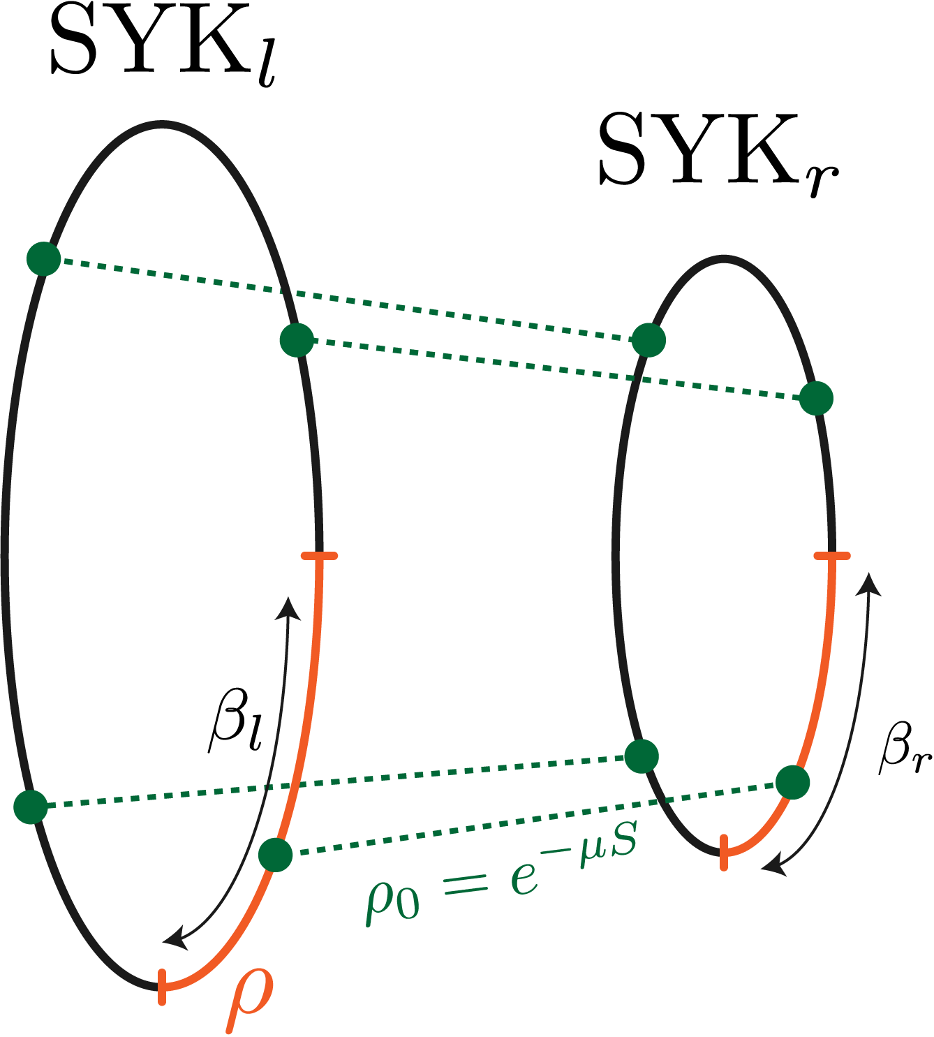
(a)

         
         

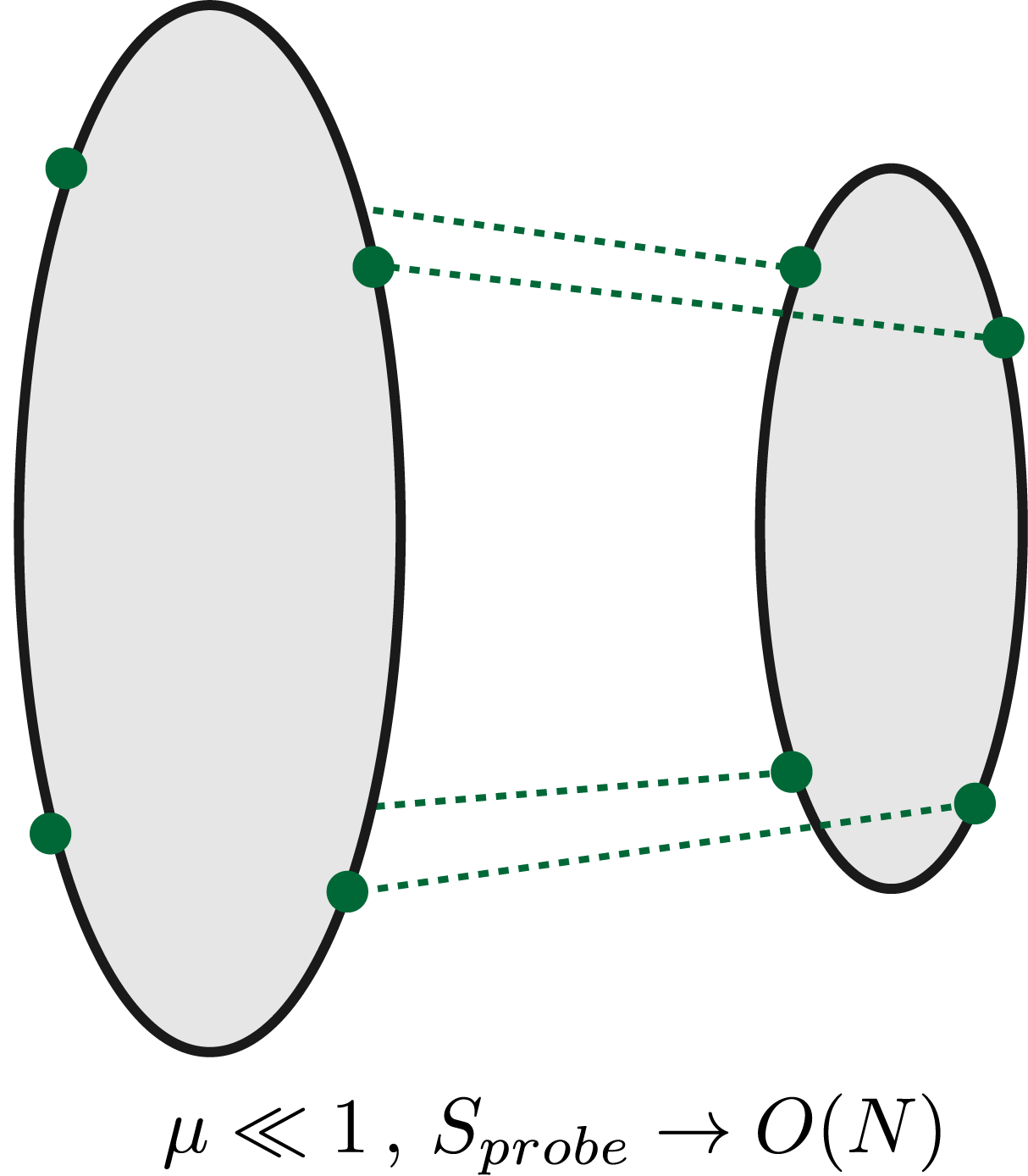
(b)

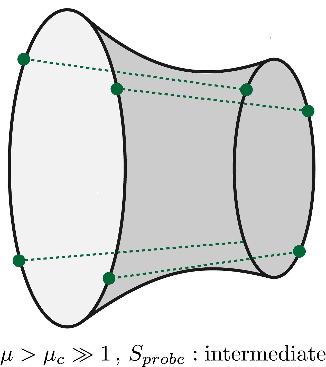
(c)

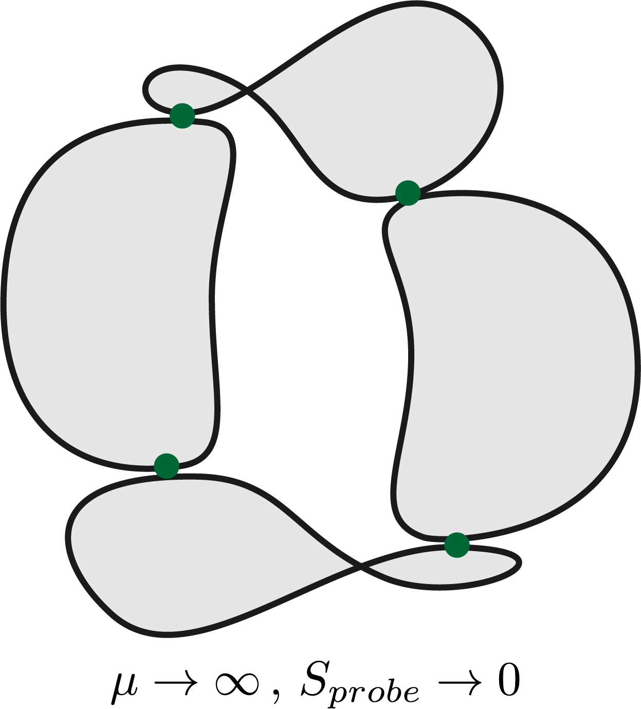
(d)

Figure 2: (a) The “necklace” SYK diagram, summarizing the replica manifold for $k=4$ replicas. The green dotted lines connecting SYK_l and SYK_r correspond to local insertions of $\rho_{0}=e^{-\mu S}$ where $S$ is the “size” operator (16) and $\mu$ a parameter related to the entropy of the probe $S_{probe}$ and defined in Section 2.1. This coupling between the two boundary quantum systems appears after we trace out the reference and is a consequence of the entanglement between the probe and the reference. The modular flowed anticommutator (2) is obtained by an analytic continuation of the SYK propagator on this “necklace” diagram. (b) The SYK “necklace” diagram serves as the boundary condition for the Euclidean path integral of the dual JT gravity. In the limit of probe entropy the dominant saddle is a pair of disconnected geometries with disk topology, leading to trivial modular flow. (c) At intermediate values of the probe entropy for $\mu$ greater than a critical value $\mu_{cr}$, the Euclidean wormhole saddle with cylindrical topology dominates, supported by the $\rho_{0}$ path integral insertions. The modular flowed commutator $W$ becomes non-trivial in this regime, allowing us to propagate into the black hole interior and detect signals sent from the other side. (d) At very small probe entropies, the backreaction of the $\rho_{0}$ becomes large, squeezing the wormhole at the insertion points, and causing it to “pinch off” into a product of $k=4$ disconnected disks with perimeter $\beta_{l}+\beta_{r}$. Modular flow becomes trivial in this limit.

In Section 4, we present the same replica computation from the perspective of the Euclidean path integral of JT gravity. In Section 4.1, we argue that the probe in the Euclidean path integral can be effectively understood as a localized injection of a fixed $SL(2,R)$ charge. The precise value of this charge constitutes UV data which we obtain from a microscopic SYK computation in Appendix D. We explicitly construct the Euclidean wormhole solution dominating in the intermediate $S_{probe}$ regime in Section 4.2 using the method developed in Stanford:2020wkf . The wormhole is supported by the localized couplings between the left and right boundaries generated by the entangling unitary $U_{sys+ref}$ after we trace out the reference. We show that the replica correlator computed in the bulk geodesic approximation exactly matches the microscopic SYK result in Section 4.3. As anticipated, the length of this wormhole is controlled by the entropy of the probe and it pinches off in the limits $S_{probe}\sim N$ and $S_{probe}\to 0$ in two different ways, as shown in Fig. 2b, 2d. It is precisely in the regime where the wormhole saddle dominates that the modular flow reliably takes us behind the horizon.

The Euclidean cylinder saddle found in Section 4 is reminiscent of the one discussed in Stanford:2020wkf and it hints, once again, at the important role played by the quenched ensemble average of the SYK couplings. Leveraging this intuition, we speculate in Section 5 on how the analogous computation may work in more general setups and higher dimensions and conclude with some thoughts on interesting future applications of this method.

2 A bulk infalling observer in SYK

2.1 Preparing the initial state

In this paper, we wish to explicitly use the tool of Jafferis:2020ora to access the behind the horizon region of two AdS₂ black holes connected by an Einstein-Rosen bridge, directly from the boundary quantum description. The first step in this process is to prepare the appropriate initial state, describing a wormhole geometry connecting two black hole exteriors, together with an “observer” inserted in the right asymptotic region whose microstates are entangled with an external reference.

An $AdS$ wormhole configuration is dual to a pair of identical holographic systems $l$ and $r$, dynamically decoupled ($H=H_{l}+H_{r}$) and in a special entangled state, the thermofield double state maldacena2013cool :

$$|\beta\rangle_{lr}\equiv\mathcal{Z}^{-\frac{1}{2}}\sum_{a}e^{-\frac{\beta E_{a}}{2}}|E_{a}\rangle_{r}|E_{a}\rangle_{l}=\mathcal{Z}^{-\frac{1}{2}}e^{-\frac{\beta}{4}H}\left|0\right\rangle_{lr}$$ (3)

where $|E_{a}\rangle_{l,r}$ are energy eigenstates of each system and $\left|0\right\rangle_{lr}$ is the maximally entangled state of the two systems obeying $(H_{l}-H_{r})\left|0\right\rangle_{lr}=0$. For simpler notation, we will omit the subscript $lr$ in $\left|0\right\rangle_{lr}$ from now on. For $AdS_{2}$, the dual boundary systems are two SYK models Maldacena:2017axo . Each SYK model is a quantum mechanical system of $N$ Majorana fermions $\psi_{l,r}^{j}$ obeying Clifford algebra

$$\{\psi_{a}^{j},\psi_{b}^{k}\}=\delta_{ab}\delta^{jk},\quad a,b=l,r.$$ (4)

The SYK Hamiltonian couples $1\ll q\ll N$ of them with coupling constants $J^{l,r}_{j_{1}\cdots j_{q}}$ which are random variables drawn from a Gaussian ensemble:

$$H_{l,r} =i^{q/2}\sum_{1\leq j_{1}<\cdots<j_{q}\leq N}J_{j_{1}\cdots j_{q}}^{l,r}\psi_{l,r}^{j_{1}}\cdots\psi_{l,r}^{j_{q}}$$ (5)

$$\mathbb{E}_{J}\left[J_{j_{1}\cdots j_{q}}^{l,r}\right] =0$$ (6)

$$\mathbb{E}_{J}\left[\left(J_{j_{1}\cdots j_{q}}^{l,r}\right)^{2}\right] =\frac{2^{q-1}\mathcal{J}^{2}(q-1)!}{qN^{q-1}}=\frac{J^{2}(q-1)!}{N^{q-1}}$$ (7)

The maximal entangled state is defined as

$$(\psi_{l}^{j}+i\psi_{r}^{j})\left|0\right\rangle=0,\quad\forall j=1,\cdots,N$$ (8)

which leads to $J_{j_{1}\cdots j_{q}}^{l}=i^{q}J_{j_{1}\cdots j_{q}}^{r}$. The state $|\beta\rangle_{lr}$ can be prepared via the standard SYK Euclidean path integral of Fig. 1a. Its holographic representation is given by the path integral of JT gravity+matter over half of the hyperbolic disk $\mathbb{H}_{2}$.

Inserting the probe

Suppose now we want to introduce a particle at the $t=0$ slice in the bulk, at some (regulated) geodesic distance $\rho$ from the right asymptotic boundary and initially at rest. We can do this simply by inserting a local operator in the path integral at a Euclidean time $\tau$ from the right endpoint (Fig. 1b)

$$|\beta,\tau\rangle_{lr}=\mathcal{Z}^{-\frac{1}{2}}\,e^{-\frac{(\beta-\tau)H_{l}}{2}}e^{-\frac{\tau H_{r}}{2}}O\,|0\rangle$$ (9)

Assuming that $O$ is dual to a bulk field with large enough mass $(1\ll m_{O}\ll N)$, the operator in (9) inserts a classical particle in the bulk path integral that will propagate along the corresponding $\mathbb{H}_{2}$ geodesic (a semi-circle), until it hits the $t=0$ slice at distance $\rho$ from right asymptotic boundary and at a normal angle. This is precisely the initial state of interest and Lorentzian evolution will propagate the particle along an infalling geodesic, like in Fig. 1b.

The formalism of Jafferis:2020ora , however, requires our probe to have a large number of microstates which are entangled with an external reference system. Since the details of the reference do not matter, we can take it, for convenience, to be a system with $N$ free Dirac fermions $c_{j}$ and $c_{j}^{\dagger}$, which we initiate in the vacuum state $|v\rangle_{ref}$. We are then interested in a state of the type:

$$|\beta,\tau\rangle_{l,r,ref}=\mathcal{Z}^{-\frac{1}{2}}\sum_{a}d_{a}\,e^{-\frac{(\beta-\tau)H_{l}}{2}}e^{-\frac{\tau H_{r}}{2}}O_{a}\,|0\rangle\,O^{ref}_{a}|v\rangle_{ref}$$ (10)

where $d_{a}$ are complex coefficients. An explicit and computationally tractable example of such a state that we will use for our analysis, is one where the desired entanglement between the system and the reference is created by a unitary $U$, generated by a bi-local fermion operator:

$$|\beta_{l},\beta_{r};\delta\rangle =\mathcal{Z}^{-\frac{1}{2}}\,e^{-\frac{\beta_{l}H_{l}}{2}}e^{-\frac{\beta_{r}H_{r}}{2}}\,U(\delta)|0\rangle|v\rangle_{ref}$$ (11)

$$U(\delta) =\exp\left[\sqrt{2}\delta\sum_{j=1}^{N}\psi^{j}_{r}(c^{\dagger}_{j}+c_{j})\right]$$ (12)

and we set $\beta_{l}=\beta-\tau$, $\beta_{r}=\tau$. This state can be expressed in the form (10) by Taylor expanding the unitary, to get:

$$|\beta_{l},\beta_{r};\delta\rangle =\mathcal{Z}^{-\frac{1}{2}}\,e^{-\frac{\beta_{l}H_{l}}{2}}e^{-\frac{\beta_{r}H_{r}}{2}}\sum_{k=0}^{N}e^{-\frac{1}{2}\mu(\delta)k}\sum_{I_{k}}\Gamma^{r}_{I_{k}}\,|0\rangle\,c^{\dagger}_{I_{k}}\,|v\rangle_{ref}$$ (13)

$$\mu(\delta) =\log\cot^{2}\delta,~{}~{}~{}~{}~{}I_{k}\equiv\{(i_{1},\cdots,i_{k})|1\leq i_{1}<\dots<i_{k}\leq N\}$$ (14)

where $c^{\dagger}_{I_{k}}\equiv c^{\dagger}_{i_{1}}\cdots c^{\dagger}_{i_{k}}$ generates fermion number basis of reference, and the Hermitian operators $\Gamma_{I_{k}}\equiv\Gamma^{a}_{i_{1}i_{2}\dots i_{k}}=2^{k/2}i^{k(k-1)}\psi_{a}^{i_{1}}\dots\psi_{a}^{i_{k}}$ for $a=l,r$ are the “size” eigenoperators of Roberts:2018mnp ; Qi:2018bje . We will regard the state as perturbation on thermofield double and thus restrict to nonnegative $\mu(\sigma)$, which is equivalent to the coupling range $\delta\in[0,\pi/4]$.

Tracing out the reference yields a reduced density matrix for the SYK${}_{l}\times$SYK_r system which reads:

$$\rho_{\beta_{l},\beta_{r},\mu} =\mathcal{Z}^{-1}\,e^{-\frac{\beta_{l}H_{l}}{2}-\frac{\beta_{r}H_{r}}{2}}\,\,\sum_{k=0}^{N}e^{-\mu(\delta)k}\sum_{I_{k}}\Gamma^{r}_{I_{k}}|0\rangle\langle 0|\Gamma^{r}_{I_{k}}\,\,e^{-\frac{\beta_{l}H_{l}}{2}-\frac{\beta_{r}H_{r}}{2}}$$

$$=\mathcal{Z}^{-1}\,e^{-\frac{\beta_{l}H_{l}}{2}-\frac{\beta_{r}H_{r}}{2}}\,\,e^{-\mu(\delta)S}\,\,e^{-\frac{\beta_{l}H_{l}}{2}-\frac{\beta_{r}H_{r}}{2}}$$ (15)

where

$$S=\frac{1}{2}\sum_{j=1}^{N}\left(1+2i\psi^{j}_{l}\psi_{r}^{j}\right)$$ (16)

is the “size” operator, defined and explored in a series of recent works Qi:2018bje ; Nezami:2021yaq ; Haehl:2021emt ; Jian:2020qpp ; Lensky:2020ubw ; Gao:2019nyj ; Lucas:2018wsc ; Schuster:2021uvg . It is clear from (15) that the entropy of probe $S_{probe}$ (which is the same as the entropy of $\rho_{\beta_{l},\beta_{r},\mu}$) is $O(N)$ for $\mu(\delta)\sim O(1)$. We are interested in probes that can be regarded as relatively small excitations of the thermofield double state, to avoid significant backreaction on the AdS₂ wormhole geometry we are trying to explore. We will, therefore, consider sufficiently small values $\delta$, however, not small enough for the excitation to be approximated by a single fermion insertion. In this case, $S_{probe}$ is intermediate as illustrated in Fig. 2c. More precisely, we will work in the limit $e^{-\mu(\delta)}\ll 1$ and $q,N,\beta\mathcal{J}\to\infty$ with $q/N\to 0$. The parametric regime in which our calculation is valid is discussed in detail in Appendix C.

2.2 Setting up the SYK computation

According to the prescription of Jafferis:2020ora , modular flow of a right exterior bulk operator $O_{r}(s)=\rho^{-is}\phi_{r}\rho^{is}$, where $\rho$ is the left-right density operator (15), translates $\phi_{r}$ along the geodesic of our infalling probe while keeping its geodesic distance from it fixed, with the modular time $s$ being proportional to the proper time along the worldline (Fig. 1c). We must emphasize that this prescription has certain important caveats discussed and resolved in Jafferis:2020ora which, however, will not be relevant in this work. A central objective of this paper is to explicitly apply this proposal to holographically reconstruct operators in the black hole interior, in SYK.

An infalling observer’s geodesic crosses the horizon of the 2-sided wormhole after a finite amount of proper time. Beyond this point, it is in causal contact with part of the left asymptotic boundary, which allows signals from the left boundary to reach our observer and influence their measurements. Such causally propagating signals are reflected in the appearance of a non-vanishing (anti-)commutator between left boundary operators $O_{l}(t)$ and right operators $O_{r}(s)$ that have been translated along the infalling geodesic.

We can, therefore, test the validity of this reconstruction in the black hole interior by computing quantum mechanically the correlator (2) with average over all Majorana fermions

$$W(s,t)=\frac{1}{N}\sum_{j=1}^{N}\text{Tr}\left(\rho\,\{\rho^{-is}\,\psi^{j}_{r}\,\rho^{is},\,\psi^{j}_{l}(t)\}\right)$$ (17)

which should be exponentially small for some finite range of $s$ and sharply reach a peak at some finite $s$. This peak signals that the flowed operator $\rho^{-is}\,\psi_{r}\,\rho^{is}$ has entered the bulk lightcone of the left boundary operator $\psi_{l}(t)$ (see Fig. 3a and 3b). More general modular flowed correlators of bulk exterior operators can be obtained from (17) by smearing the fermions in boundary time with the known HKLL kernel (see Fig. 1c and Section 3.5). As we will show, the SYK solution to (17) exactly matches semi-classical bulk computation reviewed in Section 2.3, in a parametric regime of $\beta_{l},\beta_{r},\mu$ we specify.

2.3 Bulk semiclassical expectation

We start with a discussion of what the correlation function (17) is expected to be, if the bulk interpretation of modular flow as proper time translations along the probe’s worldline in the bulk dual is correct. The two sided black holes spacetime is just a portion of global AdS₂. We can describe AdS₂ as the hypersurface Maldacena:2016upp

$$-Y_{-1}^{2}-Y_{0}^{2}+Y_{1}^{2} =-1$$ (18)

in a 3-dimensional embedding space with metric

$$ds^{2}=-dY_{-1}^{2}-dY_{0}^{2}+ dY_{1}^{2}$$ (19)

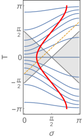
(a) $\xi=1$

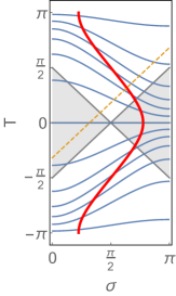
(b) $\xi=-1$

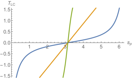
(c)

Figure 3: (a)(b) The worldline of probe (red curve) and spatial geodesics with equal $s_{p}$ separation and orthogonal to it (blue curves) in the two sided big black holes spacetime. The two shaded regions are left and right wedge respectively. The yellow dashed line is null and shot from left boundary from $T=-1$. We see clearly that the probe takes more proper time in (b) than (a) to reach the lightcone of the yellow line. (c) The location of past lightcone location $T_{LC}$ on left boundary of an atmosphere operator on right boundary after proper time $s_{p}$ evolution. Blue, yellow and green curves are for $\xi=2,0,-2$.

Parametrizing this surface as

$$Y_{-1}=\sin T\csc\sigma,\quad Y_{0}=\cos T\csc\sigma,\quad Y_{1}=-\cot\sigma$$ (20)

yields the global AdS₂ metric

$$ds^{2}=\frac{-dT^{2}+d\sigma^{2}}{\sin^{2}\sigma},\quad\sigma\in[0,\pi],\,\,\,T\in\mathbb{R}$$ (21)

The causal wedges of the left and right boundary in thermofield double state (shaded regions in Fig. 3a and Fig. 3b) only extend for $T\in[-\pi/2,\pi/2]$ and the local boundary time $t_{l,r}$ is defined as Maldacena:2016upp

$$\tan\frac{T}{2}=\tanh\frac{\pi}{\beta}t_{l,r}$$ (22)

where $\beta$ is the temperature of the thermofield double state.

AdS₂ has an $SO(2,1)$ symmetry whose embedding space representation reads:

$$M_{1}(x)=\begin{pmatrix}1&0&0\\ 0&\cosh x&\sinh x\\ 0&\sinh x&\cosh x\end{pmatrix},~{}M_{2}(y)=\begin{pmatrix}\cosh y&0&\sinh y\\ 0&1&0\\ \sinh y&0&\cosh y\end{pmatrix},~{}M_{3}(\theta) =\begin{pmatrix}\cos\theta&-\sin\theta&0\\ \sin\theta&\cos\theta&0\\ 0&0&1\end{pmatrix}$$ (23)

The simplest timelike geodesic in AdS₂ is the worldline $\sigma=\frac{\pi}{2}$. In embedding coordinates this reads $U^{\mu}Y_{\mu}=0$ for $U^{\mu}=(0,0,1)$. Any other timelike geodesic can be obtained from this one by an $SO(2,1)$ transformation

$$U^{\mu}[M_{1}]^{\kappa}_{\mu}(\xi)[M_{3}]^{\nu}_{\kappa}(c)Y_{\nu}=0,\quad$$ (24)

The general timelike geodesic can be expressed as

$$\cos\sigma=r\cos(T-c),\qquad r\in(-1,1),\,\,\,c\in[-\pi,\pi]$$ (25)

where we set $\tanh\xi=r$. The parameter $c$ sets the timeslice at which the geodesic is instantenously at rest, in the global AdS frame. For a state prepared by a Euclidean path integral over the half disk, we should take $c=0$. The limits $r\rightarrow\pm 1$ correspond to null geodesics. On the $T=c=0$ slice, positive/negative $r$ corresponds to probe starting from left/right wedge, respectively (Fig. 3a and Fig. 3b).

Proper time flow

The next step is to define a local bulk atmosphere operator by shooting a spacelike geodesic orthogonally from our probe’s worldline at the initial time, and following it for proper length $\ell$. We then want to propagate this operator along the timelike geodesic’s proper time while keeping its relative location and angle to the probe’s geodesic fixed. This is a natural choice of foliation related to the probe and is identical to the one used in Gao:2021uro for the discussion of phase space variables of JT gravity with dynamical EOW branes.

The spacelike geodesics orthogonal to $\sigma=\frac{\pi}{2}$ are $T=T_{0}$ for any $T_{0}$. In embedding space this reads $V^{\mu}Y_{\mu}=0$ with $V^{\mu}=(\cos T_{0},-\sin T_{0},0)$. An initial bulk operator located at $(T,\sigma)=(0,\sigma_{0})$ is at a geodesic distance from the probe equal to

$$\ell=\int_{\pi/2}^{\sigma_{0}}\frac{d\sigma}{\sin\sigma}=\frac{1}{2}\log\frac{1-\cos\sigma_{0}}{1+\cos\sigma_{0}}\implies\cos\sigma_{0}=-\tanh\ell$$ (26)

Propagation along the $\sigma=\frac{\pi}{2}$ geodesic for proper time $s_{p}=T_{0}$ then simply shifts the bulk operator to the global AdS point $(T_{0},\sigma_{0})$.

Propagation along a general probe’s geodesic (25) can be obtained by a simple $SO(2,1)$ transformation of the above, since AdS isometries preserve both geodesic lengths and relative angles. Restricting our attention to probes that are at rest at global time $T=0$, the AdS location of a bulk operator at distance $\ell$ from the probe, translated along the geodesic (25) for proper time $s_{p}=T_{0}$ is given by $(T_{b},\sigma_{b})$ determined by the equation

$$Y_{\mu} =[M_{1}]_{\mu}^{\nu}(\xi)Y_{\nu}^{(b)}$$

$$\Rightarrow\, (\sin T_{b}\csc\sigma_{b},\cos T_{b}\csc\sigma_{b}\cosh\xi-\cot\sigma_{b}\sinh\xi,\cos T_{b}\csc\sigma_{b}\sinh\xi-\cot\sigma_{b}\cosh\xi)$$

$$=(\sin T_{0}\csc\sigma_{0},\cos T_{0}\csc\sigma_{0},-\cot\sigma_{0}).$$ (27)

Using (26), we can solve that

$$\cot\sigma_{b} =\cos s_{p}\sinh\xi\cosh\ell-\sinh\ell\cosh\xi$$ (28)

$$\tan T_{b} =\frac{\sin s_{p}}{\cos s_{p}\cosh\xi-\tanh\ell\sinh\xi}$$ (29)

The past lightcone of this atmosphere operator meets the left boundary at $T_{LC}=T_{b}-\sigma_{b}$ which reads

$$T_{LC} =\arctan\frac{\sin s_{p}}{\cos s_{p}\cosh\xi-\tanh\ell\sinh\xi}-\arctan\frac{1}{\cos s_{p}\sinh\xi\cosh\ell-\sinh\ell\cosh\xi}$$

$$=2\arctan\left(\frac{\tan\frac{s_{p}}{2}-e^{\ell}}{e^{\xi}(1+e^{\ell}\tan\frac{s_{p}}{2})}\right)$$ (30)

where the second arctan in the first line takes values in $[0,\pi]$. We plot $T_{LC}$ as a function of proper time $s_{p}$ in Fig. 3c for an atmosphere operator near the right boundary, $\ell\rightarrow\infty$. From the plot, we see that only a finite range of $s_{p}$ leads to $T_{LC}\in[-\pi/2,\pi/2]$ as expected. Using (22), this lightcone crossing time corresponds to the left boundary time

$$t_{LC}=\frac{\beta}{\pi}\text{arctanh}\frac{\tan\frac{s_{p}}{2}-e^{\ell}}{e^{\xi}(1+e^{\ell}\tan\frac{s_{p}}{2})}$$ (31)

Matching to the path integral parameters

It is useful to express the lightcone crossing time (31) in terms of the parameters appearing in the path integral preparation of the state (Fig. 1b). For this, we need to work out the relation between $\xi$ and $\beta_{l,r}$ by considering the the purple curve in Fig. 1b as a Euclidean geodesic. To compute this, it is convenient to switch to a different global coordinate system of EAdS₂

$$ds^{2}=d\rho^{2}+\sinh^{2}\rho d\tau^{2}$$ (32)

where

$$\cosh\rho=\cosh T\csc\sigma,\quad\tan\tau=-\sinh T\sec\sigma$$ (33)

The parameter $\tau$ in (32) is an angular coordinate on $\mathbb{H}_{2}$ and it is related to the Euclidean time of the boundary path integral $\tau_{\partial}$ via:

$$\tau=\frac{2\pi\tau_{\partial}}{\beta}$$ (34)

The geodesic that is orthogonal to the $T=0$ slice at $T=0$, $\sigma=\arccos r$ is (assuming $r\in[0,1]$)

$$\frac{1+\sinh^{2}\rho\sin^{2}\tau}{(\cosh\rho+\sinh\rho\cos\tau)^{2}}=\frac{1+r}{1-r}$$ (35)

and it meets the EAdS boundary ($\rho\rightarrow+\infty$) at Euclidean time

$$\tau=\pm\pi\delta_{r}=\pm\arccos(-r)$$ (36)

where we defined $\delta_{l,r}\equiv\beta_{l,r}/\beta$. This leads to

$$\tan\pi\delta_{l}/2=\cot\frac{\arccos(-r)}{2}=\sqrt{\frac{1-r}{1+r}}=e^{-\xi}$$ (37)

where in the last step we used identity $\tanh\xi=r$.

2.4 A replica-trick for modular flowed correlators

The rest of this paper is devoted to performing the computation of (17) in two different ways and demonstrating its exact match to the bulk expectation (31) with the parameter relation (37). Both of them rely on employing a replica trick: We first consider the correlator

$$W^{k,s}_{ab}(\tau_{1},\tau_{2})=\frac{1}{N}\sum_{j=1}^{N}\text{Tr}\left[\rho^{k-s}\psi^{j}_{a}(\tau_{1})\rho^{s}\psi^{j}_{b}(\tau_{2})\right]/\text{Tr}\rho^{k}$$ (38)

where $\psi^{j}_{a}(\tau)\equiv e^{H_{a}\tau}\,\psi^{j}_{a}\,e^{-H_{a}\tau}$ and $a,b\in\{l,r\}$; we then obtain (17) from (38) via an appropriate analytic continuation in $k,s$ and $\tau_{1,2}$ with $(a,b)=(r,l)$. Here we average over all Majorana fermions in the SYK model. The replica correlator (38) corresponds the SYK propagator on the “necklace” diagram (Fig. 4). It is also important to remember that since SYK is a theory with random couplings, the correlator $W_{ab}^{k,s}$ refers to the statistical average over $J_{i_{1},i_{2},\dots,i_{q}}$ of the RHS, which we left implicit in (38). This fact will play a key role in our analysis and we will explicitly restore this ensemble average in formulas where it is important.

Before diving into the technical analysis of (38), it is illuminating to first consider two extreme limits of the computation: $\mu\to 0$ and $\mu\to\infty$.

(a) $\mu\to 0$ limit

Recalling the expression (15) for the system’s density matrix, we see that $\mu\to 0$ results in $e^{-\mu S}\to\mathbb{I}_{lr}$ and the state factorizes to a product of two thermal states for the left and right systems separately, with inverse temperatures $\beta_{l}$ and $\beta_{r}$ respectively

$$\rho_{\beta_{l},\beta_{r},\mu\to 0}\to\mathcal{Z}^{-1}e^{-\beta_{l}H_{l}}e^{-\beta_{r}H_{r}}$$ (39)

This limit corresponds to $\delta\to\frac{\pi}{4}$ in (11) which yields a maximally entangled state between the probe and the reference, with $S_{probe}\to O(N)$. The factorization of $\rho$ in this limit implies that introducing a probe with a very large entropy destroys the correlations between SYK_l and SYK_r and by extension the common geometric interior of the AdS₂ wormhole we wish to probe.

The replica correlation function of interest, i.e. (38) for $a=l$ and $b=r$, then becomes:

$$W^{k,s}_{rl}(\tau_{1},\tau_{2})\overset{\mu\to 0}{\rightarrow}\frac{1}{N\mathcal{Z}}\sum_{j=1}^{N}\mathbb{E}_{J}\left[\text{Tr}_{r}[e^{-\beta_{r}kH_{r}}\psi_{r}^{j}(\tau_{1})]\text{Tr}_{l}[e^{-\beta_{l}kH_{l}}\psi_{l}^{j}(\tau_{2})]\right]$$ (40)

where we explicitly restored the (quenched) average over the random couplings $J_{j_{1},j_{2},\dots,j_{q}}$ implicit in all SYK computations. In the bulk, the computation of (40) is dominated by the Euclidean gravitational path integral on two disconnected disks with circumferences $\beta_{l}k$ and $\beta_{r}k$ respectively (Fig. 2b), with the appropriate boundary fermion insertions on each side. This factorized contribution leads to an identically vanishing commutator (17) for all $s,t$, consistently with the expectation that inserting a large entropy probe results in a long and potentially non-geometric wormhole and, as a consequence, the probe never enters a region that can be causally influenced by the left boundary.

(b) $\mu\to\infty$ limit

The opposite limit, $\delta\to 0\Rightarrow\mu(\delta)\rightarrow\infty$, in turn, yields $e^{-\mu(\delta)S}\rightarrow\left|0\right\rangle\left\langle 0\right|$ up to normalization and $\rho_{\beta_{l},\beta_{r},\infty}$ approaches the projector onto the thermofield double state $|\beta\rangle$ with inverse temperature $\beta=\beta_{l}+\beta_{r}$:

$$\rho_{\beta_{l},\beta_{r},\mu\to\infty}\to|\beta\rangle\langle\beta|$$ (41)

The replica correlation function (38) then reduces to:

$$W^{k,s}_{rl}(\tau_{1},\tau_{2})\overset{\mu\to\infty}{\rightarrow}\begin{cases}\frac{1}{N}\sum_{j=1}^{N}\mathbb{E}_{J}\left[\langle\beta|\psi_{r}^{j}(\tau_{1})\psi_{l}^{j}(\tau_{2})|\beta\rangle\,\langle\beta|\beta\rangle^{k-1}\right]\,,\quad&\text{if: }s=0\\ \frac{1}{N}\sum_{j=1}^{N}\mathbb{E}_{J}\left[\langle\beta|\psi_{r}^{j}(\tau_{1})|\beta\rangle\langle\beta|\psi_{l}^{j}(\tau_{2})|\beta\rangle\,\langle\beta|\beta\rangle^{k-2}\right]\,,\quad&\text{if: }s\neq 0\end{cases}$$ (42)

The bulk replica computation in this regime is dominated by a product of $k$ disconnected hyperbolic disks, each having a circumference $\beta$ (Fig. 2d). Once again, this results in a vanishing commutator (17) since this is physically the case of a probe with infinitesimally small entropy $S_{probe}\to 0$ and, thus, trivial modular flow.

(c) intermediate $\mu$

The two limits above make it clear that modular flow can only be interesting in the intermediate $\mu$ regime, when the probe has an entropy that is finite but small compared to that of the ambient black hole. We can gain some intuition for the behavior of the replica correlator for finite $\mu$, by approaching it from the $\mu\to 0$ side. First notice that $W^{k,s}_{rl}$ can be expressed as

$$W_{rl}^{k,s}(\tau_{1},\tau_{2})=\frac{1}{N\mathcal{Z}}\sum_{j=1}^{N}\mathbb{E}_{J}\left[\text{Tr}[\rho^{k-s}\psi_{r}^{j}(\tau_{r})\rho^{s}\psi_{l}^{j}(\tau_{2})\right]$$

$$= \frac{1}{N\mathcal{Z}}\sum_{j=1}^{N}\mathbb{E}_{J}\left[\text{Tr}\left[{\cal T}\left\{e^{-k\beta_{l}H_{l}-k\beta_{r}H_{r}}\left(\prod_{\nu=0}^{k-1}e^{-\mu S(\nu+1/2)}\right)\psi_{r}^{j}(\tau_{1}+s\beta_{r})\,\psi_{l}^{j}(\tau_{2})\right\}\right]\right]$$ (43)

where we defined $S(x)=e^{(\beta_{l}H_{l}+\beta_{r}H_{r})x}\,S\,e^{-(\beta_{l}H_{l}+\beta_{r}H_{r})x}$ and $\psi_{l,r}^{j}(x)=e^{H_{l,r}x}\,\psi_{l,r}^{j}\,e^{-H_{l,r}x}$, the operator $S$ is the size operator defined in (16), ${\cal T}$ denotes Euclidean time ordering and the variables $\tau_{l,r}$ are restricted to the interval $\tau_{l,r}\in[0,\beta_{l,r}]$. As we take $\mu\to 0$ in (43) we explicitly recover (40).

The bulk AdS computation of (43) gets contributions from all geometries consistent with the boundary conditions set by “necklace” diagram (Fig. 2a). The two JT saddles of interest are: (a) the product of two disconnected hyperbolic geometries with disk topology and total perimeter lengths $k\beta_{l}$ and $k\beta_{r}$ respectively (Fig. 2b) and (b) the Euclidean wormhole geometry with cylindrical topology connecting the left and right boundaries (Fig. 2c). The latter is supported by the backreaction of the localized $\rho_{0}=e^{-\mu S}$ insertions, since minimizing the corresponding potential energy $V(\mu)=\mu\sum_{\nu=0}^{k-1}\langle S(\nu+1/2)\rangle$ favors large correlations between SYK_l and SYK_r. The disconnected contribution cannot give rise to a non-trivial left-right commutator after analytic continuation. It is, therefore, the Euclidean wormhole saddle that describes the physics of our probe crossing the lightcone of the left boundary fermion —when it dominates.

At small $\mu$, the insertion of $\rho_{0}$ in (43) can be expanded perturbatively about $\mu=0$, and described as the insertion of $l$-$r$ bi-local operators, of low dimension. The backreaction of these bi-locals is small and thus a Euclidean wormhole supported by them would be very long, with a large JT gravity action, hence the disconnected geometry dominates (43). The computation in large $q$ SYK model in Appendix E shows that, as $\mu$ increases, the backreaction of $\rho_{0}$ on the Euclidean geometry leads, on the one hand, to a slow and bounded decrease of the action of the disconnected contribution, and, on the other hand, to a linear decrease of the action of the wormhole contribution (Fig. 12), whose length decreases as well. At a critical value $\mu_{c}$ the two saddles exchange dominance and the dominant contribution to (43) is given by the boundary-to-boundary propagator about the Euclidean wormhole geometry of Fig. 2c. The critical value $\mu_{cr}\sim 2\beta\mathcal{J}/q^{2}$ is derived in Appendix E for the large $q$ SYK model at low temperature. In the rest of this paper, we will only focus on $\mu>\mu_{cr}$ and this connected wormhole phase.

In Section 4, we explicitly construct this bulk solution and the relevant propagator and show that its analytic continuation leads, indeed, to a modular flow consistent with the proper time translation interpretation discussed in Section 2.3. The computation breaks down for very large values of $\mu$, when the wormhole pinches off to $k$ disconnected disks (Fig. 2d).

3 Replica computation in SYK

In this Section, we perform the computation of (38) and its analytic continuation by working directly on the boundary quantum theory and finding an approximate solution to the large $q$ SYK dynamics on the “necklace” diagram (Fig. 4). We make all our approximations explicit and bound the errors in our analysis and its parametric regime of validity in Appendix C.

3.1 Large $q$ SYK on “necklace” diagram

As discussed in Section 2.1, the density matrix of interest is, up to normalization:

$$\rho=e^{-(\beta_{l}H_{l}+\beta_{r}H_{r})/2}\rho_{0}e^{-(\beta_{l}H_{l}+\beta_{r}H_{r})/2}$$ (44)

where

$$\rho_{0}\equiv\exp\left(-i\mu\sum_{j=1}^{N}\psi_{l}^{j}\psi_{r}^{j}\right)$$ (45)

We need to compute the correlation functions $W^{k,s}_{ab}(\tau_{1},\tau_{2})$ of $\psi_{a}^{j}$ (38) with $k$ copies of $\rho$ for positive integrer $k$ and nonnegative integer $s$ with $0\leq s\leq k$. This amounts to computing correlation functions on the “necklace” diagram of Fig. 4.

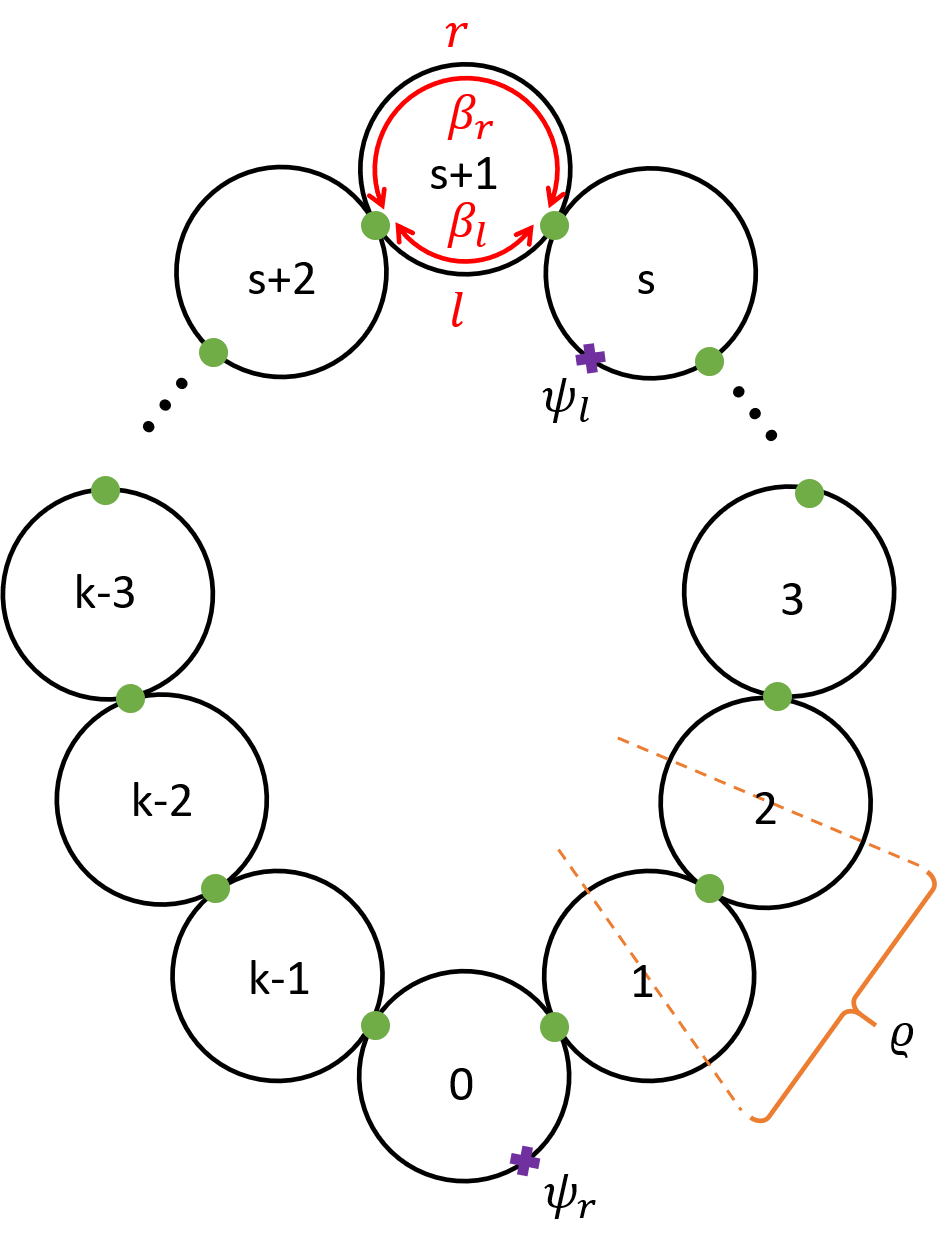
Figure 4: Necklace diagram. Splitting every circle into $l$ and $r$ on which the system evolves with SYK Hamiltonian $H_{l,r}$ respectively. Each green dot means insertion of $\rho_{0}$.

Let us first compute the correlation functions in the infinite $q$ limit, when both $l$ and $r$ SYK model Hamiltonians are zero. In this case, the correlation is only affected by the insertion of $\rho_{0}$. Therefore, the correlation function is piecewise constant and depends only on which circles the two fermions are located. The first step, it to note the following identity

$$\rho_{0}^{-1}\begin{pmatrix}\psi_{l}^{j}\\ i\psi_{r}^{j}\end{pmatrix}\rho_{0}=\begin{pmatrix}\cosh\mu&-\sinh\mu\\ -\sinh\mu&\cosh\mu\end{pmatrix}\begin{pmatrix}\psi_{l}^{j}\\ i\psi_{r}^{j}\end{pmatrix}\equiv M\begin{pmatrix}\psi_{l}^{j}\\ i\psi_{r}^{j}\end{pmatrix}$$ (46)

which means that whenever fermion crosses $\rho_{0}$, the correlation function is rotated by the matrix $M$. Let us define the 2 by 2 correlation matrix as

$$g(s)=\frac{1}{N}\sum_{j=1}^{N}\text{Tr}\left[\rho_{0}^{k-s}\begin{pmatrix}\psi_{l}^{j}\\ i\psi_{r}^{j}\end{pmatrix}\rho_{0}^{s}\begin{pmatrix}\psi_{l}^{j}\\ i\psi_{r}^{j}\end{pmatrix}^{\text{T}}\right]\bigg{/}\text{Tr}\rho_{0}^{k}$$ (47)

in which we multiplied $\psi_{r}$ by $i$ for later convenience. For $s=0$, it is clear that

$$g(0)=\begin{pmatrix}\frac{1}{2}&-x\\ x&-\frac{1}{2}\end{pmatrix}\implies g(s)=M^{s}g(0)$$ (48)

for some $x$ to be determined. The periodicity of the trace implies that

$$g(k)=M^{k}\begin{pmatrix}\frac{1}{2}&-x\\ x&-\frac{1}{2}\end{pmatrix}=g(0)^{\text{T}}=\begin{pmatrix}\frac{1}{2}&x\\ -x&-\frac{1}{2}\end{pmatrix}$$ (49)

This can be easily solved by

$$x=\frac{1}{2}\tanh\frac{k\mu}{2}$$ (50)

Plugging this solution back in (48), we have

$$g(s)=\frac{1}{2\cosh\frac{k\mu}{2}}\begin{pmatrix}\cosh\frac{(k-2s)\mu}{2}&-\sinh\frac{(k-2s)\mu}{2}\\ \sinh\frac{(k-2s)\mu}{2}&-\cosh\frac{(k-2s)\mu}{2}\end{pmatrix}$$ (51)

Now let us move on to the SYK Hamiltonian. The necklace diagram describes the Euclidean path integral of two SYK models on two different circles: the $l$ circle has circumstance of $k\beta_{l}$ and the $r$ circle has circumstance of $k\beta_{r}$. However, these two circles are not decoupled from each other. The coupling comes from two sources: one is the identical random coupling $J^{l,r}$, and the other is the localized insertion of $\rho_{0}$ after Euclidean evolution for $\beta_{l,r}$. We will adopt a hybrid treatment for these two types of couplings. For the former, we integrate over the random coupling $J^{l,r}$ and manifest the interaction between two circles; for the latter, we use (46) to transform the coupling into a specific gluing boundary condition for correlations. It is crucial that the random couplings $J^{l,r}$ are identical for all replicas and this leads to the quenched ensemble average when we integrate over $J^{l,r}$, otherwise the correlation between different replicas will be trivial. This quenched ensemble average is also important in the bulk and has been shown to be related to wormholes in recent studies Saad:2019lba ; Engelhardt:2020qpv . We will discuss more on this in Section 5.1.

After integrating over random couplings, we have the following bilocal effective action

$$S=-\frac{N}{2}\log\det(\partial_{\tau}\delta_{ab}-\Sigma_{ab})+\frac{N}{2}\int_{0}^{k\beta_{a}}d\tau\int_{0}^{k\beta_{b}}d\tau^{\prime}\left[\Sigma_{ab}(\tau,\tau^{\prime})G_{ab}(\tau,\tau^{\prime})-\frac{J^{2}}{q}s_{ab}G_{ab}(\tau,\tau^{\prime})^{q}\right]$$ (52)

where

$$s_{ab}=\begin{pmatrix}1&i^{q}\\ i^{q}&1\end{pmatrix}$$ (53)

and $G_{ab}$ is the time ordered correlation function

$$G_{ab}(\tau_{1},\tau_{2})=\frac{1}{N}\sum_{j=1}^{N}\left\langle\mathcal{T}\psi^{j}_{a}(\tau_{1})\psi^{j}_{b}(\tau_{2})\right\rangle_{necklace}$$ (54)

which has the symmetry

$$G_{ab}(\tau_{1},\tau_{2})=-G_{ba}(\tau_{2},\tau_{1})$$ (55)

It is important here to define a time ordering $\mathcal{T}$ on the “necklace” diagram, as follows. The ordering of fermions with the same subscript ($a=b$) is as usual; for those with different subscripts $a\neq b$, we first order them according to which necklace circle they are on, and in case they are on the same circle we take the ordering as it is.

Taking variations of $\Sigma$ and $G$ in (52), we have the equations of motion

$$G=(\partial_{\tau}\delta_{ab}-\Sigma_{ab})^{-1},\quad\Sigma_{ab}(\tau,\tau^{\prime})=J^{2}s_{ab}G_{ab}(\tau,\tau^{\prime})^{q-1}$$ (56)

From the definition, we see that $G_{ab}$ is related to $g_{ab}$ by appropriate factor of $i$. To have a simpler notation later, we will define a parallel version of $G_{ab}$ with $\psi_{r}\rightarrow i\psi_{r}$ and denoted by $\hat{g}_{ab}$. In the large $q$ limit, we make the standard assumption that the solution has the form

$$\hat{g}_{ab}(\tau_{1},\tau_{2})=g_{ab}(s)e^{\sigma_{ab}(\tau_{1},\tau_{2})/(q-1)},\quad s\equiv\left\lfloor\tau_{1}/\beta_{a}\right\rfloor-\left\lfloor\tau_{2}/\beta_{b}\right\rfloor\geq 0$$ (57)

whose definition for $s<0$ is given by symmetry (55). At leading order in $1/q$, the equations of motion read

$$\partial_{1}\partial_{2}\sigma_{ab}(\tau_{1},\tau_{2})\pm 2\mathcal{J}^{2}(2g_{ab}(s))^{q-2}e^{\sigma_{ab}(\tau_{1},\tau_{2})}=0$$ (58)

with $+$ sign for $ab=ll,rr$ and $-$ sign for $ab=lr,rl$. This is a piecewise Liouville equation whose general solution is

$$e^{\sigma_{ab}(\tau_{1},\tau_{2})}=\frac{f^{\prime}(\tau_{1})g^{\prime}(\tau_{2})}{\mathcal{J}^{2}(2g_{ab}(s))^{q-2}(1\pm f(\tau_{1})g(\tau_{2}))^{2}}$$ (59)

where $f$ and $g$ could be chosen differently on different circles. Any solution of the above type has an $SL(2)$ symmetry

$$f\rightarrow sl(f)\equiv\frac{a+bf}{c+df},\quad g\rightarrow sl_{\text{ad}}(g)\equiv\frac{d\mp cg}{\pm(-b\pm ag)},\quad bc-ad=1$$ (60)

We will use $\simeq$ to denote two pairs of function $(f,g)$ related by this $SL(2)$ symmetry.

Since we are looking for a piecewise solution for $\sigma_{ab}$ and translation of both fermions for integer number of circles along the “necklace” diagram does not change the solution, we will use a simpler notation by denoting $\sigma_{ab}^{s}(\tau_{1},\tau_{2})$ for $\sigma_{ab}(\tau_{1}+s\beta_{a},\tau_{2})$ where $\tau_{1,2}\in[0,\beta_{a,b}]$ from now on.

At every junction, the gluing boundary condition requires that

$$\hat{g}_{ab}(s\beta_{a+},\tau_{2}) =M_{ac}\hat{g}_{cb}(s\beta_{a-},\tau_{2}),\quad s=1,\cdots,k$$ (61)

$$\hat{g}_{ab}(\tau_{1},s\beta_{b+}) =M_{bc}\hat{g}_{ac}(\tau_{1},s\beta_{b-}),\quad s=1,\cdots,k$$ (62)

In terms of $\sigma^{s}_{ab}$, these conditions become

$$e^{\sigma^{s+1}_{aa}(0,\tau)/q_{-}}-e^{\sigma^{s}_{aa}(\beta_{a},\tau)/q_{-}} =\frac{\sinh\mu\sinh\frac{(k-2s)\mu}{2}}{\cosh\frac{(k-2(s+1))\mu}{2}}\left(e^{\sigma^{s}_{aa}(\beta_{a},\tau)/q_{-}}-e^{\sigma^{s}_{\bar{a}a}(\beta_{\bar{a}},\tau)/q_{-}}\right)$$ (63)

$$e^{\sigma^{s+1}_{a\bar{a}}(0,\tau)/q_{-}}-e^{\sigma^{s}_{a\bar{a}}(\beta_{a},\tau)/q_{-}} =\frac{\sinh\mu\cosh\frac{(k-2s)\mu}{2}}{\sinh\frac{(k-2(s+1))\mu}{2}}\left(e^{\sigma^{s}_{a\bar{a}}(\beta_{a},\tau)/q_{-}}-e^{\sigma^{s}_{\bar{a}\bar{a}}(\beta_{\bar{a}},\tau)/q_{-}}\right)$$ (64)

$$e^{\sigma^{s-1}_{aa}(\tau,0)/q_{-}}-e^{\sigma^{s}_{aa}(\tau,\beta_{a})/q_{-}} =\frac{\sinh\mu\sinh\frac{(k-2s)\mu}{2}}{\cosh\frac{(k-2(s-1))\mu}{2}}\left(e^{\sigma^{s}_{a\bar{a}}(\tau,\beta_{\bar{a}})/q_{-}}-e^{\sigma^{s}_{aa}(\tau,\beta_{a})/q_{-}}\right)$$ (65)

$$e^{\sigma^{s-1}_{a\bar{a}}(\tau,0)/q_{-}}-e^{\sigma^{s}_{a\bar{a}}(\tau,\beta_{\bar{a}})/q_{-}} =\frac{\sinh\mu\cosh\frac{(k-2s)\mu}{2}}{\sinh\frac{(k-2(s-1))\mu}{2}}\left(e^{\sigma^{s}_{aa}(\tau,\beta_{a})/q_{-}}-e^{\sigma^{s}_{a\bar{a}}(\tau,\beta_{\bar{a}})/q_{-}}\right)$$ (66)

where $\bar{a}$ means “$\neq a$” and $q_{-}\equiv q-1$. A special solution to the twist boundary condition is to assume that both the left and the right hand sides of these conditions are separately zero. This would mean that at each junction, all $\sigma_{ab}$ coincide. As we explain in Appendix A, this is impossible to achieve using the configurations (59). Nevertheless, a somewhat relaxed gluing condition of this form will be used as an approximation in Section 3.3, leading to a replica propagator that solves the SYK equations, up to a small error in the large $\beta,\mu,q$ limit.

3.2 Symmetries of $\sigma^{s}_{ab}$

In order to construct our SYK solution, it is helpful to understand the symmetries the propagator on the “necklace” diagram needs to satisfy.

First, note that $\hat{g}_{ab}$ is real, which can be easily shown using the definition of SYK Hamiltonian and $\rho_{0}$ and using the Grassmann algebra. The complex conjugate of the replica correlator then satisfies

$$\text{Tr}(\rho^{k-s}\psi_{a}(\tau_{1})\rho^{s}\psi_{b}(\tau_{2}))^{*}=\text{Tr}(\rho^{k-s}\psi_{b}(-\tau_{2})\rho^{s}\psi_{a}(-\tau_{1}))$$ (67)

which implies that

$$\sigma_{ab}^{s}(\tau_{1},\tau_{2})=\sigma_{ba}^{s}(\beta_{b}-\tau_{2},\beta_{a}-\tau_{1})$$ (68)

Physically, we can understand this condition as a KMS condition along the each circle in the “necklace” diagram. We will refer to this as the “small KMS symmetry”.

There is another symmetry for $s\neq 0,k$ which becomes evident by noting that

$$\text{Tr}(\rho^{k-s}\psi_{a}(\tau_{1})\rho^{s}\psi_{b}(\tau_{2}))=\text{Tr}(\rho^{s}\psi_{b}(\tau_{2})\rho^{k-s}\psi_{a}(\tau_{1}))$$ (69)

which implies

$$\sigma_{ab}^{s}(\tau_{1},\tau_{2})=\sigma_{ba}^{k-s}(\tau_{2},\tau_{1})$$ (70)

Together with (68) we have

$$\sigma_{ab}^{s}(\tau_{1},\tau_{2})=\sigma_{ab}^{k-s}(\beta_{a}-\tau_{1},\beta_{b}-\tau_{2})$$ (71)

Physically, we can understand this condition as a KMS condition for the whole “necklace” loop, which we dub the “big KMS symmetry”. For $s=0$ and $a\neq b$, we have

$$\text{Tr}(\rho^{k}\psi_{a}(\tau_{1})\psi_{b}(\tau_{2})) =-\text{Tr}(\rho^{k}\psi_{b}(\tau_{2})\psi_{a}(\tau_{1}))$$

$$\implies\sigma_{lr}^{0}(\tau_{1},\tau_{2}) =\sigma_{rl}^{0}(\tau_{2},\tau_{1})=\sigma_{lr}^{0}(\beta_{l}-\tau_{1},\beta_{r}-\tau_{2})$$ (72)

which extends (71) to the $s=0$ case. For the case $a=b$ becomes

$$\sigma_{aa}^{0}(\tau_{1},\tau_{2}) =\sigma_{aa}^{0}(\tau_{2},\tau_{1})$$ (73)

$$\sigma_{aa}^{0}(\tau,\tau) =0$$ (74)

$\sigma_{a}a$, however, is not smooth along $\tau_{1}=\tau_{2}=\tau$ due to the coincident fermions. Instead, we may use (73) and (74) of $\tau_{1}\geq\tau_{2}$ to define the case of $\tau_{1}\leq\tau_{2}$.

3.3 Approximate solution

The analysis of Appendix A highlights the difficulty of finding an exact large $q$ solution that satisfies all twist boundary conditions (63)-(66) and also respects all symmetries discussed in Section 3.2. We will, therefore, make a strategic retreat and look for an approximate solution, whose error will later bound.

We are interested in the regime of large $\mu$ where the correlation functions in the same circle of the “necklace”, say $s=0$, should be quite close to those in thermofield double state. We will thus build our approximate solution for finite $\mu$ by starting with the thermofield double solution ($\mu\to\infty$). A special case of our twisted boundary condition is to assume that $\sigma^{s}_{ab}$ is continuous at all junctions. This means that all LHS of (63)-(66) are zero. Of course, this condition alone does not guarantee the RHS of (63)-(66) are also zero, but we can work with this assumption regardless and confirm at the end of the computation that the violation of the twisted boundary conditions is much smaller than $1/q$ in the low temperature limit. Moreover, as analyzed in Appendix A the “big KMS symmetry” seems to be the main obstacle for obtaining an exact solution. As a fix, we construct an approximate solution by first finding a solution that violates the “big KMS symmetry” and then adding its KMS image

$$\hat{g}_{ab}(s\beta_{a}+\tau_{1},\tau_{2}) \approx g_{ab}(s)e^{\sigma_{ab}^{s}(\tau_{1},\tau_{2})/q}+g_{ba}(k-s)e^{\sigma_{ba}^{k-s}(\tau_{2},\tau_{1})/q}$$ (75)

for $0\leq s\leq k$ and then copy this solution antiperiodically for other $s$. Of course, this approximation does not solve the Liouville equation but we expect it to be very close to the real solution in the low temperature limit. A similar argument was used in Saad:2018bqo . Taking this approximation automatically satisfies the “big KMS symmetry” (70). We also show that our solution of $\sigma_{ab}^{s}$ guarantees the “small KMS symmetry” (68).

Let us first write down the solution for infinite $\mu$. In this case, $\rho_{0}$ reduces back to the projector onto the EPR state and any $s\neq 0$ correlation function is zero. For $s=0$, the correlation function is same as that in a thermofield double state with temperature $\beta=\beta_{l}+\beta_{r}$. The solution is well known

$$e^{\sigma_{ll}(\tau_{1},\tau_{2})} =e^{\sigma_{rr}(\tau_{1},\tau_{2})}=\frac{\omega^{2}}{\mathcal{J}^{2}\cos^{2}\omega(\tau_{12}-\beta/2)}$$ (76)

$$e^{\sigma_{rl}(\tau_{1},\tau_{2})} =e^{\sigma_{lr}(\tau_{1},\tau_{2})}=\frac{\omega^{2}}{\mathcal{J}^{2}\cos^{2}\omega(\tau_{1}+\tau_{2}-\beta/2)}$$ (77)

with

$$\omega=\mathcal{J}\cos\omega\beta/2$$ (78)

One can easily check that this solution satisfies the symmetries (68) and (72).

For the case of large but finite $\mu$ we may still use the aforementioned solution for $\sigma_{ab}^{0}$. To obtain the solution for $\sigma_{ab}^{s}$ in the other circles of the “necklace” we will assume continuity across the junctions

$$\sigma_{ab}^{s}(\beta_{a},\tau)=\sigma_{ab}^{s+1}(0,\tau),\quad\sigma_{ab}^{s}(\tau,0)=\sigma_{ab}^{s+1}(\tau,\beta_{b})$$ (79)

This condition is sufficient for obtaining all correlation functions, as we will show shortly. As usual, each solution $\sigma^{s}_{ab}$ of the Liouville equation is characterized by a pair of functions. By the argument of Appendix A, the continuity condition leads to the following function choices

$$\sigma_{ll}^{s}:=(f_{s},f),~{}\sigma_{rr}^{s}:=(\bar{h}_{s},h),~{}\sigma_{rl}^{s}:=(h_{s},f)$$ (80)

where all functions $f_{s},h_{s},\bar{h}_{s},f,h$ are related by SL(2) transformations. In particular, the solution (76) and (77) correspond to

$$f=h=\tan\omega\tau,\quad f_{0}=h_{0}=\bar{h}_{0}=\tan\omega(\tau-\beta/2)$$ (81)

The goal now is to use the continuity requirement to obtain this family of $SL(2,R)$ transformed functions in terms of the known $f,h,f_{0},h_{0},\bar{h}_{0}$.

$\sigma_{ll}^{s}$ and $\sigma_{rr}^{s}$

Let us first focus on $\sigma_{ll}^{s}$. We define

$$f_{s}=u_{s}+v_{s}\tan(\omega\tau+\gamma_{s}),\quad\mathcal{J}_{s}\equiv\mathcal{J}(2g_{ll}(s))^{q-2}=\mathcal{J}\left[\frac{\cosh\frac{(k-2s)\mu}{2}}{\cosh\frac{k\mu}{2}}\right]^{q-2}$$ (82)

where $\{u_{k},v_{k},\gamma_{k}\}$ are three parameters characterizing the $SL(2)$ transformation.

With this definition, we have

$$e^{\sigma_{ll}^{s}(\tau_{1},\tau_{2})}=\frac{\omega^{2}v_{s}}{\mathcal{J}\mathcal{J}_{s}(\cos(\omega\tau_{1}+\gamma_{s})(\cos\omega\tau_{2}+u_{s}\sin\omega\tau_{2})+v_{s}\sin\omega\tau_{2}\sin(\omega\tau_{1}+\gamma_{s}))^{2}}$$ (83)

The boundary condition (79) can be solved by

$$u_{s+1} =\tan(\omega\beta_{l}+\gamma_{s})-\frac{1}{2}\alpha_{s}v_{s}\sin 2\gamma_{s+1}\sec^{2}(\omega\beta_{l}+\gamma_{s})$$ (84)

$$v_{s+1} =\alpha_{s}v_{s}\cos^{2}\gamma_{s+1}\sec^{2}(\omega\beta_{l}+\gamma_{s})$$ (85)

$$\tan\gamma_{s+1} =\tan\gamma_{s}+\alpha_{s}v_{s}\sin\omega\beta_{l}\sec\gamma_{s}\sec(\omega\beta_{l}+\gamma_{s})$$ (86)

$$u_{s} =(1-v_{s})\tan(\omega\beta_{l}+\gamma_{s})$$ (87)

where

$$\alpha_{s}\equiv\mathcal{J}_{s+1}/\mathcal{J}_{s}=\left[\frac{\cosh\frac{(k-2(s+1))\mu}{2}}{\cosh\frac{(k-2s)\mu}{2}}\right]^{q-2}$$ (88)

which has symmetry $\alpha_{s}\alpha_{k-s-1}=1$. Note that in this solution, (84)-(86) are recurrence relation and (87) is a self-consistency condition for each $s$. In particular, one can check that (87) holds at every level of the recurrence if it is satisfied initially. Using (87) we can write $\sigma_{ll}^{s}$ as

$$e^{\sigma_{ll}^{s}(\tau_{1},\tau_{2})}= \frac{\omega^{2}v_{s}\cos^{2}(\omega\beta_{l}+\gamma_{s})}{\mathcal{J}\mathcal{J}_{s}\left[\cos(\omega\tau_{1}+\gamma_{s})\cos(\omega(\tau_{2}-\beta_{l})-\gamma_{s})+v_{s}\sin\omega\tau_{2}\sin\omega(\tau_{1}-\beta_{l})\right]^{2}}$$ (89)

In particular, $s=0$ corresponds to $v_{0}=1$ and $\gamma_{0}=-\omega\beta/2$. One can easily check that this solution obeys symmetry (68).

As $l$ and $r$ are identical systems, we can repeat above analysis to $\sigma_{rr}^{s}$. The solution will be the same as $\sigma_{ll}^{s}$ but with replacement $\beta_{l}\rightarrow\beta_{r}$ and parameters $\{u_{s},v_{s},\gamma_{s}\}\rightarrow\{\bar{u}_{s},\bar{v}_{s},\bar{\gamma}_{s}\}$ related to $\bar{h}_{s}$.

$\sigma_{rl}^{s}$ and $\sigma_{lr}^{s}$

Solving $\sigma_{rl}^{s}$ is quite similar. We define

$$h_{s}=\tilde{u}_{s}+\tilde{v}_{s}\tan(\omega\tau+\tilde{\gamma}_{s}),\quad\tilde{\mathcal{J}}_{s}\equiv\mathcal{J}(2g_{rl}(s))^{q-2}=\mathcal{J}\left[\frac{\sinh\frac{(k-2s)\mu}{2}}{\cosh\frac{k\mu}{2}}\right]^{q-2}$$ (90)

Taking ansatz (90) into (59), we have

$$e^{\sigma_{rl}^{s}(\tau_{1},\tau_{2})}=\frac{\omega^{2}\tilde{v}_{s}}{\mathcal{J}\tilde{\mathcal{J}}_{s}(\cos(\omega\tau_{1}+\tilde{\gamma}_{s})(\cos\omega\tau_{2}-\tilde{u}_{s}\sin\omega\tau_{2})-\tilde{v}_{s}\sin\omega\tau_{2}\sin(\omega\tau_{1}+\tilde{\gamma}_{k}))^{2}}$$ (91)

The boundary condition (79) can be solved by

$$\tilde{u}_{s+1} =\cot\omega\beta_{l}-\cos\gamma_{s}\csc\omega\beta_{l}\sec(\omega\beta_{r}+\tilde{\gamma}_{s})-\frac{1}{2}\tilde{\alpha}_{s}\tilde{v}_{s}\sec^{2}(\omega\beta_{r}+\tilde{\gamma}_{s})\sin 2\tilde{\gamma}_{s}$$ (92)

$$\tilde{v}_{s+1} =\tilde{\alpha}_{s}\tilde{v}_{s}\cos^{2}\tilde{\gamma}_{s+1}\sec^{2}(\omega\beta_{r}+\tilde{\gamma}_{s})$$ (93)

$$\tan\tilde{\gamma}_{s+1} =\tan\tilde{\gamma}_{s}-\tilde{\alpha}_{s}\tilde{v}_{s}\sin\omega\beta_{l}\sec\tilde{\gamma}_{s}\sec(\omega\beta_{r}+\tilde{\gamma}_{s})$$ (94)

$$\tilde{u}_{s} =\cot\omega\beta_{l}-\cos\tilde{\gamma}_{s}\csc\omega\beta_{l}\sec(\omega\beta_{r}+\tilde{\gamma}_{s})-\tilde{v}_{s}\tan(\omega\beta_{r}+\tilde{\gamma}_{s})$$ (95)

where

$$\tilde{\alpha}_{s}\equiv\tilde{\mathcal{J}}_{s+1}/\tilde{\mathcal{J}}_{s}=\left[\frac{\sinh\frac{(k-2(s+1))\mu}{2}}{\sinh\frac{(k-2s)\mu}{2}}\right]^{q-2}$$ (96)

which has symmetry $\tilde{\alpha}_{s}\tilde{\alpha}_{k-s-1}=1$. Again, in this solution, (92)-(94) are recurrence relation and (95) is a self-consistency condition for each $s$. Using (95) we can write $\sigma_{rl}^{s}$ as

$$e^{\sigma_{rl}^{s}(\tau_{1},\tau_{2})}= \frac{\omega^{2}\tilde{v}_{s}\cos^{2}(\omega\beta_{r}+\tilde{\gamma}_{s})\sin^{2}\omega\beta_{l}}{\mathcal{J}\tilde{\mathcal{J}}_{s}}\left[\cos(\omega\tau_{1}+\tilde{\gamma}_{s})(\cos\tilde{\gamma}_{s}\sin\omega\tau_{2}\right.$$

$$\left.-\cos(\omega\beta_{r}+\tilde{\gamma}_{s})\sin\omega(\tau_{2}-\beta_{l}))-\tilde{v}_{s}\sin\omega\beta_{l}\sin\omega\tau_{2}\sin\omega(\tau_{1}-\beta_{r})\right]^{-2}$$ (97)

In particular, $s=0$ corresponds to $\tilde{v}_{0}=1$ and $\tilde{\gamma}_{0}=-\omega\beta/2$.

To get $\sigma_{lr}^{s}$, we can simply use symmetry (68). However, we also need to check this procedure is consistent with our boundary condition (79) that defines above recurrence sequence. This turns out to be the case simply because (79) also respects the symmetry (68). In other words, taking $ab=rl$ in (79) together with the symmetry (68) exactly leads to $ab=lr$ in (79).

Approximate solution of recurrence

Solving these recurrence relations exactly and in closed form is a difficult task. Instead, we will leverage the observation that these recurrence sequences converge very fast and can be well approximated by their continuous version which are second order differential equations. Solving the differential equations leads to an approximate solution of the recurrence sequence and also offers a closed form which is required for the subsequent analytic continuation we want to perform. We perform this computation in Appendix B and present the result here.

Let us define the recurrence variables

$$y_{s} =\frac{\cos(\omega\beta_{l}+\gamma_{s})}{\cos\gamma_{s}},\quad x_{s}=v_{s}\sec^{2}\gamma_{s},\quad\lambda=\sin^{2}\omega\beta_{l}$$ (98)

$$\tilde{y}_{s} =\frac{\cos(\omega\beta_{r}+\tilde{\gamma}_{s})}{\cos\tilde{\gamma}_{s}},\quad\tilde{x}_{s}=\tilde{v}_{s}\sec^{2}\tilde{\gamma}_{s},\quad\tilde{\lambda}=\sin\omega\beta_{l}\sin\omega\beta_{r}$$ (99)

Their continuous versions obeying the aforementioned differential equations are denoted by exchanging the subscript $s$ for a variable $s$, e.g. $y_{s}\rightarrow y(s)$ etc. In the large $\mu$ limit, the solution is

$$y(s) =\begin{cases}\alpha^{1/2}\exp[c_{1}\coth(c_{1}s+b_{1})]&s\leq\left\lfloor k/2\right\rfloor\\ \alpha^{-1/2}\exp[c_{2}\coth(c_{2}s+b_{2})]&s>\left\lfloor k/2\right\rfloor\end{cases}$$ (100)

$$x(s) =\begin{cases}\frac{x_{0}\sinh^{2}b_{1}}{\sinh^{2}(c_{1}s+b_{1})}&s\leq\left\lfloor k/2\right\rfloor\\ \frac{x_{0}\sinh^{2}b_{1}\sinh^{2}(c_{2}\left\lfloor k/2\right\rfloor+b_{2})}{\sinh^{2}(c_{1}\left\lfloor k/2\right\rfloor+b_{1})\sinh^{2}(c_{2}s+b_{2})}&s>\left\lfloor k/2\right\rfloor\end{cases}$$ (101)

$$\tilde{y}(s) =\begin{cases}\alpha^{1/2}\exp[\tilde{c}_{1}\tanh(\tilde{c}_{1}s+\tilde{b}_{1})]&s\leq\left\lfloor k/2\right\rfloor\\ \alpha^{-1/2}\exp[\tilde{c}_{2}\tanh(\tilde{c}_{2}s+\tilde{b}_{2})]&s>\left\lfloor k/2\right\rfloor\end{cases}$$ (102)

$$\tilde{x}(s) =\begin{cases}\frac{\tilde{x}_{0}\cosh^{2}\tilde{b}_{1}}{\cosh^{2}(\tilde{c}_{1}s+\tilde{b}_{1})}&s\leq\left\lfloor k/2\right\rfloor\\ \frac{\tilde{x}_{0}\cosh^{2}\tilde{b}_{1}\cosh^{2}(\tilde{c}_{2}\left\lfloor k/2\right\rfloor+\tilde{b}_{2})}{\cosh^{2}(\tilde{c}_{1}\left\lfloor k/2\right\rfloor+\tilde{b}_{1})\cosh^{2}(\tilde{c}_{2}s+\tilde{b}_{2})}&s>\left\lfloor k/2\right\rfloor\end{cases}$$ (103)

in which $\alpha\equiv e^{-\mu(q-2)}\approx e^{-\mu q}$ and other parameters are defined as

$$c_{1} =\log(y_{\infty}/\alpha^{1/2}),\quad b_{1}=\text{arccoth}(\log(y_{0}/\alpha^{1/2})/\log(y_{\infty}/\alpha^{1/2}))$$ (104)

$$c_{2} =\log(y_{\infty}\alpha^{1/2}),\quad b_{2}=\text{arccoth}\left(\frac{\log\alpha+c_{1}\coth(c_{1}\left\lfloor k/2\right\rfloor+b_{1})}{c_{2}}\right)-c_{2}\left\lfloor k/2\right\rfloor$$ (105)

$$\tilde{c}_{1} =\log(\tilde{y}_{\infty}/\alpha^{1/2}),\quad\tilde{b}_{1}=\text{arctanh}(\log(\tilde{y}_{0}/\alpha^{1/2})/\log(\tilde{y}_{\infty}/\alpha^{1/2}))$$ (106)

$$\tilde{c}_{2} =\log(\tilde{y}_{\infty}\alpha^{1/2}),\quad\tilde{b}_{2}=\text{arctanh}\left(\frac{\log\alpha+\tilde{c}_{1}\tanh(\tilde{c}_{1}\left\lfloor k/2\right\rfloor+\tilde{b}_{1})}{\tilde{c}_{2}}\right)-\tilde{c}_{2}\left\lfloor k/2\right\rfloor$$ (107)

where $y_{\infty}$ and $\tilde{y}_{\infty}$ are limit values of recurrence sequences for which a closed form is presented in (233) and (231). However, their exact formula is not needed since they can reliably be approximated as $y_{1}$ and $\tilde{y}_{1}$ in large $\beta$ and small $\alpha$ limit.

In terms of $x(s)$, $y(s)$, $\tilde{x}(s)$ and $\tilde{y}(s)$, the large $q$ solution becomes

$$g_{ll}(s) e^{\sigma_{ll}^{s}(\tau_{1},\tau_{2})/q}=\frac{1}{2}\left(\omega\lambda\mathcal{J}^{-1}x(s)^{1/2}y(s)[(\sin\omega(\beta_{l}-\tau_{1})+y(s)\sin\omega\tau_{1})\right.$$

$$\left.\times(\sin\omega\tau_{2}+y(s)\sin\omega(\beta_{l}-\tau_{2}))-\lambda x(s)\sin\omega\tau_{2}\sin\omega(\beta_{l}-\tau_{1})]^{-1}\right)^{2/q}$$ (108)

$$g_{rl}(s) e^{\sigma_{rl}^{s}(\tau_{1},\tau_{2})/q}=\frac{\text{sgn}(g_{rl}(s))}{2}\left(\omega\tilde{\lambda}\mathcal{J}^{-1}\tilde{x}(s)^{1/2}\tilde{y}(s)[(\sin\omega(\beta_{r}-\tau_{1})+\tilde{y}(s)\sin\omega\tau_{1})\right.$$

$$\left.\times(\sin\omega\tau_{2}+\tilde{y}(s)\sin\omega(\beta_{l}-\tau_{2}))+\tilde{\lambda}\tilde{x}(s)\sin\omega\tau_{2}\sin\omega(\beta_{r}-\tau_{1})]^{-1}\right)^{2/q}$$ (109)

For $\sigma_{rr}^{s}$ and $\sigma_{lr}^{s}$, we can simply switch $\beta_{l}\leftrightarrow\beta_{r}$. Note that to get $\sigma_{lr}^{s}$, we can also use symmetry (68), which turns out to be the same as the swap $\beta_{l}\leftrightarrow\beta_{r}$.

It is worth recalling at this point, that the solution we obtained above is an approximate one, in a number of different ways. First and foremost, this solution does not exactly satisfy the twisted gluing conditions at the junctions of the “necklace” diagram. In Appendix B, we confirm that the errors of this approximation, namely the deviation of the RHS of (63)-(66) from zero, are much smaller than $1/q$ in the large $\mu,\beta$ limit (see Fig. 11). In Appendix C, we present a further systematic analysis of the errors introduced by all the approximations we make, in order to justify the validity of our solution in large $\mu,\beta$ limit.

3.4 Analytic continuation

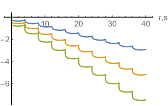
Figure 5: The plot of $\sigma_{rl}^{s}(\tau,\beta_{l}/2)/q$, where different $s$ are joined together in order. Blue, yellow and green curves are for $\mathcal{J}=20,200,2000$ respectively. We see the correlation decays exponentially as $s$ increases and the decay is stronger when we increase $\mathcal{J}$. Here other parameters are $\beta_{l}=1$, $\beta_{r}=4$, $\alpha=1/500$, $q=20$ and $k=9$.

Let us now return to the physical question of interest. The quantity we want to compute is the causal correlator (17), which we restate for convenience

$$W(s,t)=\frac{1}{N}\sum_{j=1}^{N}\text{Tr}\left(\rho\{\rho^{-is}\psi^{j}_{r}\rho^{is},\psi^{j}_{l}(t)\}\right)$$ (110)

The right SYK operator is evolved with the modular Hamiltonian $\rho^{is}$ — which is expected to be the SYK dual of the proper time evolution along the infalling probe’s worldline. The anti-commutator with the left boundary insertion is intended to detect the moment $\rho^{-is}\psi_{r}\rho^{is}$ crosses the bulk lightcone of $\psi_{l}(t)$ in the wormhole interior.

The causal propagator can be obtained from the imaginary part of Euclidean “necklace” diagram correlation function $\hat{g}_{rl}$ we computed in the previous Section

$$W(s,t)=2\Im\hat{g}_{rl}(is\beta_{r}+\beta_{r}/2,it+\beta_{l}/2)$$ (111)

To obtain this imaginary part, we need to analytically continue two parameters, $k$ and $s$. We do this using the following prescription. We first analytically continue $s$ to pure imaginary $is$ while keeping $k$ a positive odd integer greater than 1. Then we continue $k$ to $1$. Taking $s\rightarrow is$ first means that we should take the $s<\left\lfloor k/2\right\rfloor$ case of our $x,y,\tilde{x},\tilde{y}$ for $\sigma_{ab}^{s}$ and the other case for $\sigma_{ab}^{k-s}$ in (75). Then taking $k\rightarrow 1$ sets $\left\lfloor k/2\right\rfloor=0$ which leads to

$$b_{2} =\text{arccoth}(\log(y_{0}\alpha^{1/2})/\log(y_{\infty}\alpha^{1/2}))$$ (112)

$$\tilde{b}_{2} =\text{arctanh}(\log(\tilde{y}_{0}\alpha^{1/2})/\log(\tilde{y}_{\infty}\alpha^{1/2}))$$ (113)

The causal correlator $W(s,t)$ then reads:

$$W(s,t) =2\Im g_{rl}(is)\left(e^{\sigma_{rl}^{is}(\beta_{r}/2,\beta_{l}/2+it)/q}+e^{\sigma_{rl}^{1-is}(\beta_{r}/2,\beta_{l}/2-it)/q}\right)$$

$$= \Im\left(\frac{\omega\tilde{\lambda}\tilde{x}(is)^{1/2}\tilde{y}(is)/(\mathcal{J}\sin\omega\beta_{r}/2)}{(1+\tilde{y}(is))(\sin\omega(\beta_{l}/2+it)+\tilde{y}(is)\sin\omega(\beta_{l}/2-it))+\tilde{\lambda}\tilde{x}(is)\sin\omega(\beta_{l}/2+it)}\right)^{2/q}$$

$$+(t\leftrightarrow-t,\tilde{x}(is)\leftrightarrow\tilde{x}(1-is),\tilde{y}(is)\leftrightarrow\tilde{y}(1-is))$$ (114)

where for $\tilde{x}(is)$ and $\tilde{y}(is)$ we use $\tilde{c}_{1},\tilde{b}_{1}$ and for $\tilde{x}(1-is)$ and $\tilde{y}(1-is)$ we use $\tilde{c}_{2},\tilde{b}_{2}$. Only the first term in (114) is important because the second term becomes small in low temperature limit where $\beta_{l,r}$ are both large (or equivalently $\mathcal{J}$ is large). This can be seen already in the plot of the Euclidean correlator before analytic continuation in Fig. 5. In this plot, the amplitude of correlation function decreases when we increase (the real part of) $s$.

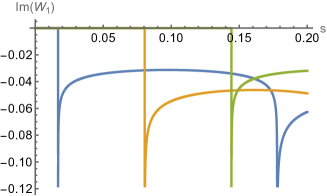
(a)

(b)

(c)

(d)

Figure 6: The plot of $\Im W_{1,2}(s,t)$ with different $t$. Blue, yellow and green curves are with $t=-3,0,3$ respectively. The parameters for (a) and (b) are $\beta_{l}=1,\beta_{r}=4$ (injection is in left side) and for (c) and (d) are $\beta_{l}=4,\beta_{r}=1$ (injection is in right side). Other parameters are $\alpha=10^{-5}$, $\mathcal{J}=10^{6}$ and $q=12$.

We can separate the two lines in (114) before taking imaginary part and denote them as $W_{1}$ and $W_{2}$ respectively. We plot their imaginary part in Fig. 6. $\Im W_{2}$ is generally smaller than $\Im W_{1}$ as expected, therefore, we can ignore it in the large $\mathcal{J},\mu$ limit. The analysis of Appendix C offers the following more accurate statement: $|W_{2}/W_{1}|\ll 1$ if $\frac{\beta\mathcal{J}\alpha^{1/2}}{\pi}\sin\pi\delta_{l}=\eta$ for $\eta\ll 1$, $\eta\gg 1$ and $|\eta-1|\ll 1$, where we assume $\delta_{l}\sim O(1)$. In other words, if $\beta\mathcal{J}$ and $\alpha^{-1/2}=e^{\mu q/2}$ are separate large scales or, alternatively, they are both large and fine tuned, $W_{2}$ becomes negligible.

There is another reason we should ignore $W_{2}$ that at $s=0$ the imaginary part of $W$ should be zero for any $t$. Clearly, $W_{1}$ obeys this rule as one can see it by plugging in the value of $\tilde{x}(0)$ and $\tilde{y}(0)$ from (197) and (198) but $W_{2}$ does not (unless $t=0$). This is an artifact of introducing the image for correlator. But in some large $\mathcal{J},\mu$ limit, this violation is small so we may expect our approximation close to true solution in this regime. This is similar to Saad:2018bqo where the image term is ignored in computation of the ramp of form factor in SYK model because it involves a long time.

The key observation is the existence of very sharp peaks of $\Im W_{1}$ at specific finite modular times $s$. In the bulk dual these should be interpreted as the infalling proper times at which $\psi_{r}$ enters the light-cone of the left boundary insertion $\psi_{l}(t)$. In particular, as we increase $t$, the location of peak moves towards large $s$, which is an important feature consistent with this interpretation. Furthermore, the blue curve in Fig. 6a has two peaks. If we plot $\Im W_{1}$ for a larger range of $s$, we will see periodic peaks for all different $t$. We should interpret these periodic peaks as $\psi_{r}$ entering the light-cone of $\psi_{l}(t)$ many times because the AdS boundary condition reflects null rays from $\psi_{l}(t)$ between two boundaries, causing the modular flowed operator to cross its lightcone an infinite number of times.

The location of the peak and the bulk lightcone

We can compute the location of peaks in the expectation value of the modular flowed commutator as follows. In the low temperature/strong coupling limit, we see that the sequence $\tilde{y}_{s}$ converges to its limit value extremely fast, Fig. 10. We can, therefore, replace $\tilde{y}_{\infty}$ with $\tilde{y}_{1}$ without affecting the result. Focusing on large SYK coupling $\mathcal{J}$, we can obtain the solution

$$\omega =\frac{\pi}{\beta}\left(1-\frac{2}{\beta\mathcal{J}}+O(1/\beta^{2}\mathcal{J}^{2})\right)$$ (115)

$$\tilde{y}_{0} \approx\frac{\beta\mathcal{J}}{\pi}\sin\pi\delta_{l},\quad\tilde{y}_{1}\approx\tilde{y}_{0}(1+\alpha),\quad\tilde{y}_{s}\approx\tilde{y}_{s-1}(1+O(\alpha(\alpha\tilde{y}_{0}^{-2})^{s-1}))$$ (116)

$$\tilde{x}_{0} \approx\beta^{2}\mathcal{J}^{2}/\pi^{2},\quad\tilde{x}_{s}\approx O(\alpha(\alpha\tilde{y}_{0}^{-2})^{s-1})$$ (117)

Note that the last equation estimates how close $\tilde{y}_{1}$ to $\tilde{y}_{\infty}$ in the small $1/\mathcal{J}$ and $\alpha$ limit. Using this formula, we have

$$\tilde{c}_{1}\approx\log\left(\frac{\beta\mathcal{J}}{\pi\alpha^{1/2}}\sin\pi\delta_{l}\right),\quad\tilde{b}_{1}\approx\frac{1}{2}\log(\tilde{c}_{1}/\alpha)$$ (118)

which are both large numbers. This means that the analytically continued function $\tilde{y}(is)$ is oscillating very quickly and with a small amplitude around a large mean value $\tilde{y}(0)$. Therefore, we can simply replace all $\tilde{y}(is)$ as $\tilde{y}_{0}$ in $W_{1}$ and get

$$W_{1}(s,t)\approx\left(\frac{(2\pi\sin\pi\delta_{l}/2)/(\beta\mathcal{J})}{X(s)\sin\omega(\beta_{l}/2-it)+X(s)^{-1}\sin\omega(\beta_{l}/2+it)}\right)^{2/q}$$ (119)

where

$$X(s)=\cos\tilde{c}_{1}s+i\tanh\tilde{b}_{1}\sin\tilde{c}_{1}s\rightarrow e^{i\tilde{c}_{1}s}$$ (120)

where, in last step, we also took the large $\tilde{b}_{1}$ limit as suggested by (118). With this approximation, we see clearly that $W_{1}$ is real for small $s$ until the denominator vanishes at modular time

$$s=\frac{1}{2\tilde{c}_{1}}\left(\pi+2\arctan\frac{\tanh\pi t/\beta}{\tan\pi\delta_{l}/2}+2\pi\mathbb{N}\right)$$ (121)

which determines the location of the peaks in Fig. 6a and Fig. 6c. Here $2\pi\mathbb{N}$ counts for all periodic peaks.

In the following, we only focus on the first peak that corresponds to choosing $0\in\mathbb{N}$. Clearly, (121) is a monotonically increasing function of $t$ as expected. For $t=0$, the peak location is fixed at $s=\pi/(2\tilde{c}_{1})$ and is independent on the value of $\delta_{l}$. This feature is also illustrated by the yellow curves in Fig. 6a and Fig. 6c, where the slight distinction is due to subleading corrections. On the other hand, taking a reflection $t\rightarrow-t$ flips the value of $s$ symmetrically around $\pi/(2\tilde{c}_{1})$.

This result matches exactly with the bulk expectation Fig. 3c in Section 2.3. Indeed, the $\ell\rightarrow\infty$ limit of (31) reduces to (121), if we identify

$$s=\frac{1}{2\tilde{c}_{1}}s_{p}$$ (122)

According to Jafferis:2020ora , the modular time parameter $s$ should be interpreted as the bulk proper time in units of the inverse temperature of probe black hole $\beta_{probe}/(2\pi)$. The matching condition above defines the effective temperature of our probe, produced by the entangling unitary (12) in Section 2.1, which reads:

$$\beta_{probe}=4\pi\tilde{c}_{1}=4\pi\log\left(\frac{\beta\mathcal{J}}{\pi\alpha^{1/2}}\sin\pi\delta_{l}\right)$$ (123)

This offers an explicit confirmation of the validity of the proposal of Jafferis:2020ora in the setup explored in this work.

A feature of our SYK result that is at odds with the proposal of Jafferis:2020ora , when taken at face value, is the fact that the modular flow associated with the probe we initiated in the right exterior gives consistent results even when it is used to evolve SYK_l operators (see Fig. 6a) This is far outside the expected regime of validity of the modular time/proper time connection: The arguments presented in Jafferis:2020ora only guarantee a coincidence of the two operators when acting on operators in the vicinity of the probe. The reason for the extended regime of validity of the prescription in our setup is the emergent SL$(2,R)$ symmetry of SYK which underlies the solution for the modular flowed correlator we studied.

3.5 Bulk fields behind horizon

In the previous Subsection we studied the modular flow of a right boundary Majorana fermion; this is an operator at an infinite geodesic distance $\ell\to\infty$ from the infalling probe’s worldline. We can generalize the discussion to the modular flow of a bulk field at a finite distance $\ell$ from the probe.

We can achieve this by expressing a bulk fermion, localized in the right exterior region on the initial $T=0$ slice, in terms of boundary fermions using the usual HKLL reconstruction Hamilton:2005ju ; Hamilton:2006az ; Hamilton:2006fh . The metric in the right Rindler wedge of eternal AdS₂ black hole reads

$$ds^{2}=d\rho^{2}-\left(\frac{2\pi}{\beta}\right)^{2}\sinh^{2}\rho dt^{2}$$ (124)

and the bulk spinor field is expressed as an integral over the Majorana operators of SYK_r as

$$\chi(\rho,t)=\int_{D(t_{*})}dt^{\prime}K(\rho,t;t^{\prime})\psi_{r}(t^{\prime})$$ (125)

where the integral range $D(t_{*})=[-t_{*},t_{*}]$ only includes the boundary time-strip that is spacelike separated from $(\rho,t)$. In for $t^{\prime}\in D(t_{*})$, $K(\rho,t;t^{\prime})$ is a real function. See Fig. 1c as an illustration. The relevant AdS₂ kernel, at leading order in $1/N$, was derived in Lensky:2020ubw .

The modular flow of the bulk spinor $\chi$ is

$$\chi_{s}(\rho,t)\equiv\rho^{-is}\chi(\rho,t)\rho^{is}=\int_{D(t_{*})}dt^{\prime}K(\rho,t;t^{\prime})\rho^{-is}\psi_{r}(t^{\prime})\rho^{is}$$ (126)

Let us take $t=0$ and some arbitrary finite $\rho$. After an amount $s$ of evolution with the infalling modular Hamiltonian, the causal correlation between $\chi_{s}(\rho,0)$ and $\psi_{l}(t)$ reads

$$\left\langle\{\chi_{s}(\rho,0),\psi_{l}(t)\}\right\rangle=\int_{D(t_{*})}dt^{\prime}K(\rho,0;t^{\prime})\cdot 2\Im\left(g_{rl}(is)e^{\sigma_{rl}^{is}(\beta_{r}/2+it^{\prime},\beta_{l}/2+it)/q}\right)$$ (127)

where we have, once again, omitted the sum over “big KMS” images in the SYK result for the commutator. Even without using the specific form of $K$, we can already read off the modular time at which the commutator (127) becomes nonzero: It is the value of $s$ for which the largest $t^{\prime}$ hits the lightcone of left insertion $\psi_{l}(t)$. Using the same approximation as (119), we have

$$\hat{W}(s,t;t^{\prime}) \equiv 2\Im\left(g_{rl}(is)e^{\sigma_{rl}^{is}(\beta_{r}/2+it^{\prime},\beta_{l}/2+it)/q}\right)$$

$$=\Im\left(\frac{(\pi\sin\pi\delta_{l})/(\beta\mathcal{J})}{e^{is_{p}/2}\cos\omega(\beta_{l}/2-it^{\prime})\sin\omega(\beta_{l}/2-it)+c.c}\right)^{2/q}$$ (128)

A bulk spinor located at distance $\ell$ away from the probe on the $T=0$ slice, is located at the AdS₂ point (28) and (29) with $s_{p}=0$. This operator is supported on the asymptotic boundary over the time strip $D(t_{*})$ with

$$t_{*}=\frac{\beta}{\pi}\text{arctanh}(e^{\xi-\ell})$$ (129)

On the other hand, the pole of $\tilde{W}(s,t;t_{*})$ is at

$$\Re\left(e^{is_{p}/2}\sin\omega(\beta_{r}/2+it_{*})\sin\omega(\beta_{l}/2-it)\right)=0$$ (130)

which can be solved to find:

$$t=\frac{\beta}{\pi}\text{arctanh}\frac{\tan\frac{\pi\delta_{l}}{2}\tanh\frac{\pi t_{*}}{\beta}\tan\frac{s_{p}}{2}-1}{\cot\frac{\pi\delta_{l}}{2}\tan\frac{s_{p}}{2}+\tanh\frac{\pi t_{*}}{\beta}}=\frac{\beta}{\pi}\text{arctanh}\frac{\tan\frac{s_{p}}{2}-e^{\ell}}{e^{\xi}(1+e^{\ell}\tan\frac{s_{p}}{2})}$$ (131)

where we used (37) and (129) in the second step. This result exactly matches with bulk expectation (31).

Locality of bulk modular flow

Using (128), we can show that modular flow preserves the locality of the field $\chi(\rho,t)$ in the bulk. The key fact is that, in the regime where (128) is valid, our modular flow reduces to an $SL(2)$ isometry $U(s)$ of AdS₂. Specifically, it is the symmetry that fixes a particular timelike bulk geodesic (what we referred to previously as our probe’s trajectory) and moves $\chi$ from $(\rho,t)$ to $U(s)(\rho,t)$ with reference to that geodesic, just as described in section 2.3

$$\chi_{s}(\rho,t)=\chi(U(s)(\rho,t))$$ (132)

In embedding coordinates, this $U(s)$ transformation can be expressed in a simple way

$$U(s)\cdot Y=M_{1}(\xi)^{-1}\cdot M_{3}(-s_{p})\cdot M_{1}(\xi)\cdot Y$$ (133)

where $M_{i}$ are given by (23).

To understand why this is so, note that bulk correlation functions between two points, $Y_{a}$ and $Y_{b}$, in AdS₂ are functions of geodesic length $\ell$ between them which is, in turn, given by $\cosh\ell=-Y_{a}\cdot Y_{b}$. One can easily show that (128) is proportional to $(-Y_{a}\cdot U(s)\cdot Y_{b})^{-2/q}$, with $Y_{a}$ at the left AdS boundary and $Y_{b}$ at the right, using the Rindler coordinate representation for $Y_{\mu}$

$$Y_{-1}=\sinh\rho\sinh\frac{2\pi}{\beta}t,~{}~{}Y_{0}=\cosh\rho,~{}~{}Y_{1}=\pm\sinh\rho\cosh\frac{2\pi}{\beta}t$$ (134)

where plus (minus) sign is for left (right) Rindler wedge. Now recall that the HKLL reconstruction of a bulk field is uniquely determined by the mode expansion of the dual boundary operator and the bulk equation of motion. Since the latter is invariant under $SL(2)$ isometry, the modular evolution of a boundary operator $\psi$ is uniquely extended to that of a bulk field and, therefore, acts on it exactly as (132).

4 Replica computation in EAdS₂

In this section, we compute the modular flowed commutator (17) using the replica trick (38) for the bulk JT gravity path integral. As discussed in Section 2.4, there are two classical geometries that contribute to the replica correlator $W_{ab}^{k,s}(\tau_{1},\tau_{2})$, shown in Fig. 2b and 2c. However, only the Euclidean wormhole contribution can lead to a non-trivial anticommutator between $\psi_{l}(t)$ and $\rho^{-is}\psi_{r}\rho^{is}$. We, therefore, start by constructing the relevant bulk wormhole saddle. We then compute the boundary-to-boundary propagator in this geometry and analytically continue it to obtain the desired anticommutator $W(s,t)$, finding exact agreement with (121). In Appendix E we specify the parameter regime in which the wormhole saddle is indeed the dominant contribution, deriving the regime of validity of our path integral analysis.

4.1 The replica path integral in JT gravity

Our starting point will be expression (43) for the finite $\mu$ replica correlator of interest which we repeat here for convenience

$$W_{rl}^{k,s}(\tau_{1},\tau_{2})=\frac{1}{N\mathcal{Z}}\sum_{j=1}^{N}\mathbb{E}_{J}\left[\text{Tr}[\rho^{k-s}\psi_{r}^{j}(\tau_{r})\rho^{s}\psi_{l}^{j}(\tau_{2})\right]$$

$$= \frac{1}{N\mathcal{Z}}\sum_{j=1}^{N}\mathbb{E}_{J}\left[\text{Tr}\left[{\cal T}\left\{e^{-k\beta_{l}H_{l}-k\beta_{r}H_{r}}\left(\prod_{\nu=0}^{k-1}e^{-\mu S(\nu+1/2)}\right)\psi_{r}^{j}(\tau_{1}+s\beta_{r})\,\psi_{l}^{j}(\tau_{2})\right\}\right]\right]$$ (135)

The head-on holographic computation of (135) in the large $\mu$ regime we are interested in is tricky. The difficulty lies in pinning down the precise deformation to the JT gravity action introduced by the potential term $\mu\sum_{\nu=0}^{k-1}S(\nu+1/2)$ when $\mu\gg 1$. We will make progress by exploiting the fact that the insertions of $\rho_{0}=e^{-\mu S}$ are localized on the boundary. This means that the bulk gravity action is the standard JT action, describing the familiar Schwarzian dynamics of a pair of boundary particles, almost everywhere in the bulk, except in the region near the $\rho_{0}$ insertions which have the physical effect of pulling the two boundary particles closer together, as discussed in Section 2.4. Such localized kicks of the boundary particle’s trajectory can be effectively parametrized by the change they induce in its $SL(2,R)$ charge. Focusing on the effect of $\rho_{0}$ on this charge amounts to looking only at its gravitational backreaction. The precise value of the $SL(2,R)$ charge $M$ associated to each insertion $\rho_{0}$, however, is UV information that needs to be computed microscopically using an SYK analysis.

Our strategy for this computation will, therefore, be the following: We look for a solution of pure JT gravity with a cylindrical topology, connecting two boundaries of total renormalized proper lengths $k\beta_{l}$ and $k\beta_{r}$, respectively, with $k$ localized insertions of $\rho_{0}$ at the appropriate points which we effectively treat as kicks with $SL(2,R)$ Casimir $M$. This yields a geometry that depends on the parameters $\beta_{l},\beta_{r},k$ and $M$. We compute the boundary-to-boundary propagator for fermions at arbitrarty replica separations $s$ in this geometry using the geodesic approximation and analytically continue it to $k\to 1$ and $s\to is$ to obtain the modular flowed correlator of interest. Finally, we use the microscopic solution of the previous Section to evaluate our effective charge $M$ in terms of the SYK parameters $\mu,{\cal J},q$ and import it in the solution. The final result for the modular flowed correlator precisely matches the SYK computation of the previous Section.

4.2 The Euclidean wormhole solution

Since any solution to the JT gravity equations is locally hyperbolic, the wormhole solution we are looking for can be understood as a patch of $\mathbb{H}_{2}$, endowed with the topology of a cylinder by a subsequent identification with respect to an isometry of $\mathbb{H}_{2}$. Our goal is, therefore, to identify the right patch of EAdS₂ and the relevant isometry used to compactify it. The appropriate patch and its identification is shown in Fig. 7.

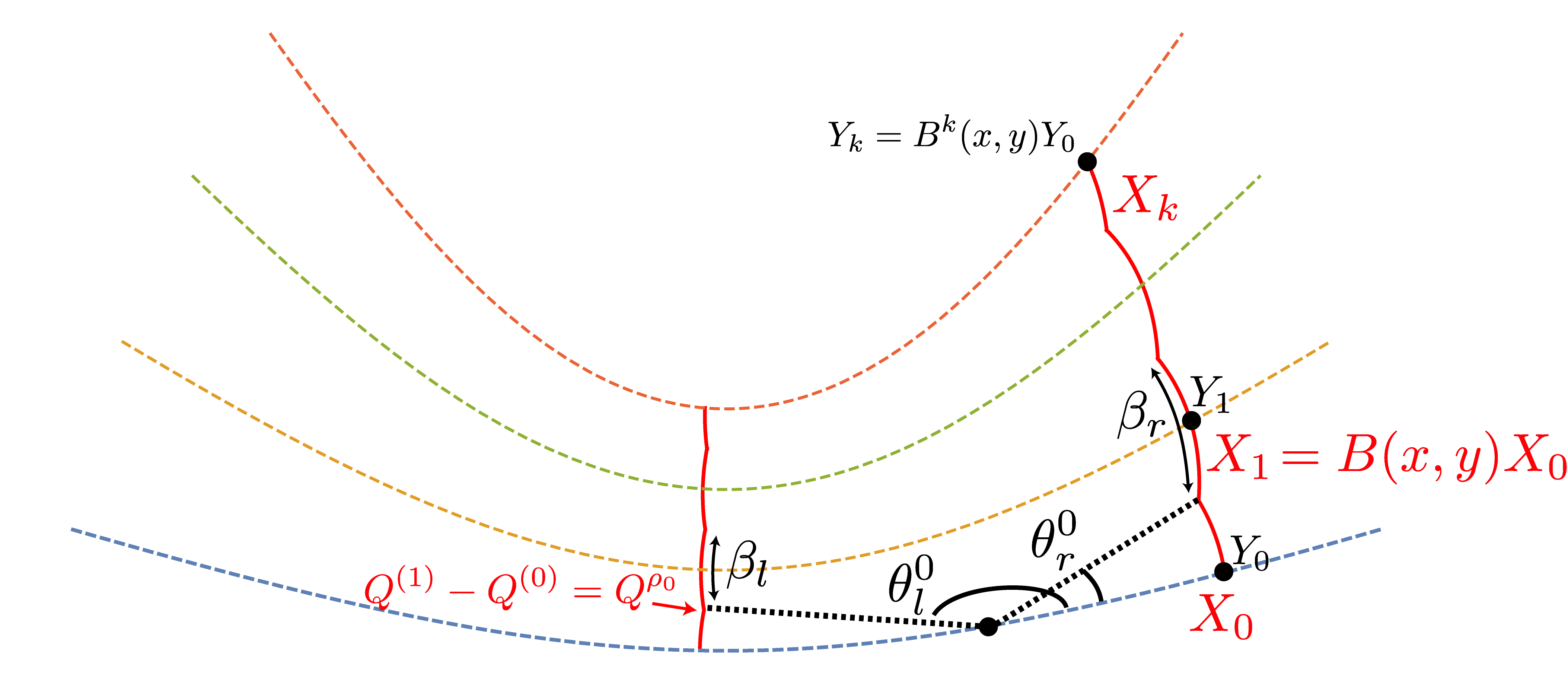
Figure 7: The Euclidean wormhole geometry dominating the bulk JT path integral with “necklace” diagram boundary conditions at intermediate values of $S_{probe}$, constructed from the patch of the hyperbolic plane $\mathbb{H}_{2}$ between the two solid red curves. Each red colored segment is an arc of a circle $X_{n}$, $n=0,1,\dots k$ (147), which are related to each other via iterative applications of the $SL(2,R)$ transformation $B(x,y)$ (144). Blue, yellow, green and red dashed curves are hyperbolic geodesics that define the diameters of each circles $X_{n}$, whose intersection with $X_{n}$ is chosen as angular starting point $Y_{n}$ of each circle respectively. The boost parameters $x,y$ and the radius $\rho$ of the circles are fixed by demanding that the arc lengths between circle intersections are $\beta_{l}$ and $\beta_{r}$ for the left and right boundaries respectively, and that the local kicks at the intersections, caused by the attractive force exerted by the $\rho_{0}$ insertions, correspond to changes of the boundary’s $SL(2,R)$ charge by an amount $Q^{\rho_{0}}$, with $(Q^{\rho_{0}})^{2}=-M^{2}$ being UV data obtained from a microscopic SYK calculation (Appendix D) and given by (159). The cylindrical topology is obtained by taking the quotient of $\mathbb{H}_{2}$ with respect to the action of $B^{k}(x,y)$, essentially identifying the geodesic diameters defining $Y_{0}$ and $Y_{k}$.

The rules of the construction are simple and were already discussed in Stanford:2020wkf . The JT dynamics in our case describes a pair of boundary particles that propagate according to the Schwarzian dynamics for proper lengths $\beta_{l}$ and $\beta_{r}$, respectively, before getting interrupted by a local insertion of $\rho_{0}$. Forgetting about the effect of the latter for the moment, the solution of the Euclidean Schwarzian equations of motion is well known and it describes a circular boundary particle trajectory in EAdS₂. Using the embedding space coordinate of EAdS₂

$$X_{0}^{\mu}(\theta)=\{\sinh\rho\sin\theta,\sinh\rho\cos\theta,\cosh\rho\}$$ (136)

with the same $(-,-,+)$ signature metric (19), this trajectory can be written as

$$X_{0}^{\mu}(\theta)Q^{(0)}_{\mu}=\frac{1}{2\epsilon},~{}\epsilon\to 0$$ (137)

with $SL(2,R)$ charge

$$Q^{(0)}_{\mu}=\{0,0,\frac{1}{2\epsilon\cosh\rho}\}$$ (138)

where the radius of the circle $\rho$ is meant to be taken to infinity simultaneously with $\epsilon\to 0$ so that:

$$2\pi\epsilon\sinh\rho\to\beta_{E}$$ (139)

The remaining parameter $\beta_{E}$ characterizes the solution and is related to the energy of the state via the thermodynamic relation $\beta_{E}=\frac{\pi^{2}}{E^{2}}$.

In the case at hand, this circular trajectory is interrupted by the $\rho_{0}$ insertions. To understand their effect, let us first select a diameter of $X_{0}$, intersecting with $X_{0}$ at two points with one point labelled as $Y_{0}$, with respect to which we will measure angular locations. It turns out that for coordinate given in (137), we can choose $\theta=0$ for $Y_{0}$. Starting from $Y_{0}$, the left and right boundary particles are initiated at $\theta=\pi$ and $\theta=0$, respectively, and then propagate along the two converging circular arcs of $X_{0}$ for proper lengths $\beta_{l}/2$ and $\beta_{r}/2$. At that point, their evolution is modified by the presence of $\rho_{0}$ which, as explained in Stanford:2020wkf , acts as a “kick” on both left and right boundary trajectories with $SL(2,R)$ Casimir $M$. The kick makes them start moving along arcs of a new EAdS circle $X_{1}$, which intersects $X_{0}$ at the location of the insertion but whose $SL(2,R)$ charge is shifted by the charge of the operator, $Q^{(1)}_{\mu}=Q^{(0)}_{\mu}+Q^{\rho_{0}}_{\mu}$, where $(Q^{\rho_{0}})^{2}=-M^{2}$. See Fig. 7 as an illustration.

Since all circles on hyperbolic space are related by $SL(2,R)$ transformations, this new circular trajectory can be described as:

$$X^{\mu}_{1}(\theta)=[B(x,y)]^{\mu}_{\nu}X^{\nu}_{0}(\theta)$$ (140)

where $B(x,y)$ is some 2-parameter element of $SL(2,R)$. As all circles are defined as the first equation of (137), it is equivalent to say that the new circular trajectory is defined with the new charge $Q^{(1)}=Q^{(0)}\cdot B(x,y)$. The reason for the 2-parameters $x,y$ is that together with $\beta_{E}$ they account for the 3 physical parameters of our problem, $\beta_{l},\beta_{r},M$. The goal is then to determine the precise transformation $B(x,y)$ and the value of $\beta_{E}$ given $\beta_{l},\beta_{r},M$.

Gluing conditions

The conditions on $B(x,y)$ and $\beta_{E}$ are simple to describe: (a) The intersection points of $X_{1}$ with $X_{0}$ must be at angular locations $\theta^{l,r}_{0}$ (with respect to starting point $Y_{0}$) such that the corresponding (renormalized) arc lengths of $X_{0}$ match the left and right inverse temperature parameters $\beta_{l,r}$ (Fig. 7):

$$\frac{\beta_{E}}{2\pi}\theta^{r}_{0} =\frac{\beta_{r}}{2}$$ (141)

$$\frac{\beta_{E}}{2\pi}(\pi-\theta^{l}_{0}) =\frac{\beta_{l}}{2}$$ (142)

and (b) the $SL(2,R)$ charge must be conserved at the intersection point, which can be ensured by:

$$\left(Q^{(0)}\cdot B(x,y)-Q^{(0)}\right)^{2}=-M^{2}$$ (143)

The boundary particles will then begin to follow $X_{1}$ starting from its intersection points with $X_{0}$, located at angular locations $\theta_{1}^{r}=-\theta_{0}^{r}$ and $\theta_{1}^{l}=-\theta_{0}^{l}$ (with respect to the starting point $Y_{1}=B(x,y)\cdot Y_{0}$ of $X_{1}$) for proper lengths $\beta_{r}$ and $\beta_{l}$ before encountering another operator insertion with a similar effect. The same story will then be repeated $k$ times.

The two conditions above can be satisfied by the $SL(2,R)$ transformation:

$$B(x,y)=M_{1}(-x)\cdot M_{2}(y)\cdot M_{1}(x)$$ (144)

where the generators $M_{i}$, $i=1,2,3$ of $SL(2,R)$ in embedding space were defined in (23). Taking (144) into (143), we have

$$\cosh x\sinh\frac{y}{2}=\frac{\beta_{E}M}{2\pi}$$ (145)

The intersections of the circles $X_{0}(\theta_{0})$ and $X_{1}(\theta_{1})$ are at the angular locations $\theta_{0}^{r,l}$ that solve the equation:

$$\coth(y/2)=\cosh x\coth\rho\csc\theta_{0}^{r,l}+\sinh x\cot\theta_{0}^{r,l}$$ (146)

Setting $\theta_{0}^{r,l}$ equal to (142) amounts to 2 constraints on the 3 undetermined parameters of our solution $x,y$ and $\rho$ (equivalently $\beta_{E}$) in terms of $\beta_{l},\beta_{r}$. The last constraint that allows us to solve the system comes from further imposing (145).

Iterating the procedure $k$ times is straightforward, by virtue of the homogeneity of EAdS₂: The sequence of $SL(2,R)$ transformed circles

$$X_{n}=B^{n}(x,y)\cdot X_{0}=M_{1}(-x)\cdot M_{2}(ny)\cdot M_{1}(x)\cdot X_{0}\,,\quad n=0,\dots k-1$$ (147)

are guaranteed to intersect each other at angular locations $\theta_{n}^{r,l}=\pm\theta_{0}^{r,l}$ (with respect to the $n$-th starting point $Y_{n}=B^{n}\cdot Y_{0}$) ensuring that the proper length of the arcs $I^{r}_{n}=[-\theta_{n}^{r},\theta_{n}^{r}]$ and $I^{l}_{n}=[\theta_{n}^{l},2\pi-\theta_{n}^{l}]$, $n=1,\dots,k-1$ between subsequent intersections is always $\beta_{r}$ and $\beta_{l}$ respectively. Fig. 7 shows the resulting patch of EAdS relevant for a wormhole with $k=3$.

Compactification

The final step, is to compactify this patch of hyperbolic space to obtain a solution with cylindrical topology. This is, also, straightforward since the entire configuration was constructed by subsequent applications of an $SL(2,R)$ transformation: We simply identify the diameter defining $Y_{0}$ of the initial circle $X_{0}$ with the diameter defining $Y_{k}=B^{k}(x,y)Y_{0}$ of the final one $X_{k}$ —namely, we quotient $\mathbb{H}_{2}$ by the action of $B^{k}(x,y)=M_{1}(-x)\cdot M_{2}(ky)\cdot M_{1}(x)$. This completes the construction of the Euclidean wormhole saddle of the replica JT path integral.

4.3 Modular flowed correlator

Having constructed the Euclidean wormhole solution, we can return to the computation of

$$W_{rl}^{k,s}(\tau)=\text{Tr}[\rho^{k-s}\psi_{r}\rho^{s}\psi_{l}(\tau)]$$ (148)

and we will take $s<k/2$ without loss of generality. The boundary correlator of conformal dimension $\Delta$ is given by $\propto\cosh^{-\Delta}\ell$ where $\ell$ is the geodesic distance of two boundary points Maldacena:2017axo . We can account for the cylindrical topology of the bulk configuration by employing the method of images:

$$W_{rl}^{k,s}(\tau)\sim\sum_{m=0}^{\infty}\frac{1}{\cosh^{\Delta_{\psi}}\ell(P^{(0)}_{l}(\tau),P_{r}^{(s+mk)})}+\sum_{m=0}^{\infty}\frac{1}{\cosh^{\Delta_{\psi}}\ell(P^{(0)}_{l}(\tau),P_{r}^{(k-s+mk)})}$$ (149)

where $\ell(\cdot,\cdot)$ is the length of the shortest geodesic connecting the 2 points in the Euclidean wormhole, ${\Delta_{\psi}}=1/q$ is the dimension of a Majorana fermion and $P_{l,r}^{(m)}$ are the embedding space coordinates of the left or right fermion insertions on the “necklace” diagram:

$$P^{(0)}_{l}(\tau) =X_{0}(\pi-\tau)\,,\quad\tau\in[-\theta_{0}^{r},\theta_{0}^{r}]$$ (150)

$$P^{(m)}_{r} =X_{m}(0)=B^{m}(x,y)X_{0}(0)$$ (151)

The second term in (149) that involves $k-s$ separation of “necklace circles” comes from the geodesics connecting two boundary point from the other circular direction on cylindrical topology. This is the same idea we used to sum over images in (75) in order to ensure the “big KMS symmetry”. As in the SYK computation of Section 4, let us focus on the dominant contribution to (149) which, after the final analytic continuation to $k\to 1$ $s\to is$, comes from the shortest wormhole geodesic, $\ell(P_{l}^{(0)}(\tau),P_{r}^{(s)})$. As long as $M\ll N$, we can approximate the length of the latter by the embedding space formula $\cosh\ell(P^{(0)}_{l},P_{r}^{(s)})=P^{(0)}_{l}\cdot P_{r}^{(s)}$ and the replica 2-point function becomes

$$W_{rl}^{k,s}(\tau)\approx\frac{1}{(X_{0}(\pi-\tau)\cdot B^{s}(x,y)\cdot X_{0}(0))^{\Delta_{\psi}}}\,,\quad\tau\in[-\theta_{0}^{r},\theta_{0}^{r}]$$ (152)

Since the dependence of the function (152) on the replica separation $s$ is through $M_{2}(sy)$, which is analytic in $s$, we can directly continue $k\to 1$, $s\to is$ and $\tau\rightarrow 2\pi it/\beta_{E}$. After a straightforward computation, the modular flowed correlation function under the limit of (139) is

$$W(s,t) =2^{-{\Delta_{\psi}}}\left(\frac{\beta_{E}\mathcal{J}}{2\pi}\right)^{-2{\Delta_{\psi}}}\left(e^{-x}\cos\frac{ys}{2}\cosh\frac{\pi t}{\beta_{E}}+\sin\frac{ys}{2}\sinh\frac{\pi t}{\beta_{E}}\right)^{-2{\Delta_{\psi}}}$$ (153)

wehre we removed the overall factor proportional to $\epsilon^{2\Delta_{\psi}}$ as a normalization choice. Here the replica-symmetric wormhole geometry parameters $x,y,\beta_{E}$ are fixed by the parameters $\beta_{l},\beta_{r},\mu$ of the SYK state via the conditions discussed in the previous Section. In the large $\beta_{E}$ limit, the latter admit the simple solution:

$$\theta_{0}^{l} =\theta_{0}^{r}\iff\beta_{E}=\beta_{l}+\beta_{r}$$ (154)

$$\tanh x \approx\cos\left(\frac{\pi\beta_{l}}{\beta_{E}}\right)\Rightarrow e^{-x}=\tan\frac{\pi\delta_{l}}{2}$$ (155)

$$\sinh\frac{y}{2} \approx\frac{\beta_{E}M}{2\pi}\frac{1}{\cosh x}\Rightarrow y\sim 2\log\frac{\beta_{E}M\sin\pi\delta_{l}}{\pi}$$ (156)

where we defined $\delta_{l}=\beta_{l}/\beta_{E}$ similarly as before. Note that (155) exactly matches (37) of the semiclassical particle analysis so the wormhole parameter $x$ corresponds to the boost parameter $x=\xi$.

The modular flowed 2-sided correlation function (153) will develop a branch cut and thus give rise to a non-trivial anticommutator (17) at the modular time:

$$s=\frac{2}{y}\text{arccot}\left(-e^{x}\tanh\frac{\pi t}{\beta_{E}}\right)=\frac{2}{y}\left[\pi+\text{arctanh}\left(\frac{\tanh\frac{\pi t}{\beta_{E}}}{\tan\frac{\pi\delta_{l}}{2}}\right)\right]$$ (157)

which exactly matches with (121), with the identification of $y$ with $\tilde{c}_{1}/2$ and $\beta_{E}$ with $\beta$. This determines the probe’s effective temperature to be

$$\beta_{probe}=2\pi y\approx 4\pi\log\frac{\beta_{E}M\sin\pi\delta_{l}}{\pi}$$ (158)

This value of $\beta_{probe}$ is consistent with the SYK expression for the normalization of the probe’s clock (123), after matching the $SL(2,R)$ charge $M$ to the SYK parameter

$$M=\mathcal{J}e^{\mu q/2}$$ (159)

This precise value of the $SL(2,R)$ charge (159) introduced by $\rho_{0}$, which was deduced here from consistency, can indeed be obtained directly from a microscopic SYK computation, as we show in Appendix D. The $SL(2,R)$ charge of $\rho_{0}$ increases as we dial up $\mu$, consistent with the expectation that as $\mu\to\infty$, $\rho_{0}$ approaches a projector onto the maximally entangled state between $l$ and $r$ causing the wormhole to pinch off and split into $k$ disconnected disks (Fig. 2d).

5 Discussion

5.1 Lessons for a general prescription for interior reconstruction

In this paper, we utilized the framework of Jafferis:2020ora in order to holographically reconstruct the degrees of freedom hidden behind the horizon of an $AdS_{2}$ black hole in Jackiw-Teitelboim gravity. Our motivation for this investigation was twofold: (a) provide an explicit application of the proposed interior reconstruction method in a setup that is under technical control and (b) identify the key ingredients of the computation that can clarify the relation of our approach to other interior reconstruction techniques, and may additionally offer clues for how to successfully apply the prescription in more interesting setups involving higher dimensional and possibly single-sided black holes.

Entanglement with reference couples the two exteriors via modular flow

The first noteworthy aspect of our construction that distinguishes it from previous works is the fact that we do not deform the boundary dynamics of the system in order to access the interior. It is well understood that turning on an explicit coupling between the two boundaries can lead to traversable wormholes Gao:2016bin that allow some left excitations to causally reach the right boundary after a finite time Gao:2018yzk ; Maldacena:2017axo . Explicit couplings between the two sides can also be utilized in the AdS₂/SYK correspondence to construct approximate SYK duals of the bulk $SL(2,R)$ symmetry generators which can transport operators behind the horizon Lin:2019qwu . Our conceptual contribution lies in demonstrating that the interior can be explored without such boundary Hamiltonian deformations, or even reference to a second asymptotic region.

Our construction, instead, relies on introducing a bulk probe whose microstates we entangle with an external reference. The preparation of this initial state is all the information we need to define the operator $\rho^{is}$ which transports local operators in relation to the bulk worldline our probe follows. We are essentially using the relative phases between our holographic system and the reference as an internal “clock” which allows us to specify the location of operator insertions in the bulk. This clock is relational in nature and is distinct from the boundary clock generated by the SYK Hamiltonians.

It is, of course, true that the modular flow couples SYK_l and SYK_r which is why we can get a non-trivial anti-commutator $\{\psi_{l},\rho^{-is}\psi_{r}\rho^{is}\}$ after sufficient $s$. However, this coupling is not an input but instead a consequence of the entanglement between our holographic system and the reference. The initial state determines the coupling between the 2 sides —we are not allowed to pick it by hand. This two-sided coupling appearing in modular flow after tracing out a subsystem is reminiscent of the discussion of Chandrasekaran:2021tkb .

The conceptual advantage of this perspective is highlighted by imagining an application of our reconstruction to single-sided black hole interiors. In this case, there exist no second microscopic system describing a second exterior wormhole region; we have a single holographic CFT in a high energy state. The Hamiltonian deformation that could move us into the interior —the analog of the $SL(2,R)$ generators of Lin:2019qwu — becomes unclear in this case (though see Kourkoulou:2017zaj ; DeBoer:2019yoe ; Brustein:2018fkr and the recent interesting work Leutheusser:2021qhd for suggestions) but our approach carries over unchanged. The situation is similar for 2-sided holographic systems in states dual to very long wormholes, where the 2-sided coupling required for propagating to the interior is exponentially complex Bouland:2019pvu , or for the case of AdS black holes evaporating into an external reservoir, where the interior becomes part of the “entanglement island” of the radiation system at sufficiently long times. Hence, the application of our method to the aforementioned setups appears to us to be a very promising avenue for future work.

At this point, it is important to point out that the interior reconstruction method we explored is highly non-linear: Every initial state we prepare our system in, provides us with a generally different operator $\rho^{is}$, after tracing out the reference. This extreme non-linearity leads to a number of problems when one attempts to apply our prescription starting from general initial states. These problems were discussed in Jafferis:2020ora and can be successfully addressed, as will be explained in an upcoming work LamprouJafferisdeBoer .

Chaos and universality of the effective coupling

Both microscopic and Euclidean JT path integral analysis highlight the role of the emergent $SL(2,R)$ symmetry of the IR sector of SYK: The generator of the probe’s modular flow effectively reduced, in the appropriate parameter regime, to an element of this $SL(2,R)$ algebra. This symmetry is only approximate and provides an effective description of the maximally chaotic dynamics of the quantum theory. In particular, the $SL(2,R)$ algebra can be organized into a boost element $B$ and its two eigen-operators, $P_{\pm}$ with eigenvalues $\pm i$

$$[B,P_{\pm}]=\pm iP_{\pm}\,,\quad[P_{+},P_{-}]=iB$$ (160)

which grow exponentially under the boost flow $e^{iBt}$. Holographically, $B$ is linked to the IR action of SYK Hamiltonian, while $P_{\pm}$ characterize the exponentially growing disruption of correlations caused by small perturbations as a function of boundary time, due to the so-called scrambling phenomenon in chaotic systems Lin:2019qwu . In fact, this very symmetry was the key principle that guided the construction of the effective theory of maximal chaos of Blake:2021wqj ; Blake:2017ris .

The prominent role of the $SL(2,R)$ symmetry in determining our modular flow, therefore, hints at a possible universality of the SYK modular evolution that takes us into the black hole interior —a universality established by maximal chaos. As explained above, entangling a probe introduced in the right asymptotic region to a reference system results in a modular flow that couples the two asymptotic regions of the wormhole, after tracing out the reference. Maximal chaos then appears to imply a particular universal form for this effective coupling which is largely independent of the precise details of the probe we introduced: its scrambling “potential”, characterized by the amount of $SL(2,R)$ charge the coupling injects, determines all the useful information about the modular flow, at least in the setup analyzed in this work, where all details of the exact microscopic coupling just amounts to tuning the value of the $SL(2,R)$ charge. It would be interesting to understand if maximal scrambling leads to a similarly universal modular flow in higher dimensions and whether it provides an avenue for connecting our approach to that of Leutheusser:2021qhd and DeBoer:2019yoe .

Ensemble average and operator randomness

The third important element of our construction was the quenched ensemble average over SYK couplings. In the microscopic treatment this was important for obtaining the Liouville equations dictating the fermion propagation on the “necklace” diagram, while it entered our bulk discussion via the appearance of the Euclidean wormhole saddle between the two boundaries.

In an attempt to understand the physical role of this averaging in more general situations, let us return to our original setup from Section 2.1: A thermofield double state of a pair of $0-$dimensional holographic quantum systems dual to an $AdS_{2}$ wormhole, which we entangle with an external reference in the completely general state

$$|\beta,\tau\rangle_{l,r,ref}=\mathcal{Z}^{-\frac{1}{2}}\sum_{i}d_{i}\,e^{-\frac{\beta_{l}H_{l}}{2}}e^{-\frac{\beta_{r}H_{r}}{2}}O_{i}\,|0\rangle\,O^{ref}_{i}|v\rangle_{ref}$$ (161)

where again $|0\rangle$ is the maximally entangled state of the two systems and written in energy basis is

$$\left|0\right\rangle\propto\sum_{\alpha}\left|E_{\alpha}\right\rangle_{l}\left|E_{\alpha}\right\rangle_{r}$$ (162)

This time, however, we will not make any specific choice of operator basis, $O_{i}$, as we did in the main text. Instead, we will treat the operators $O_{i}$ as random matrices within an energy window $E\in[0,E_{cut}]$ with $E_{cut}\lesssim O(N)$. This is motivated by the Eigenstate Thermalization Hypothesis (ETH) DAlessio:2015qtq , according to which the energy basis matrix elements $[O_{i}]_{\alpha\bar{\alpha}}$ of simple operators $O_{i}$ in a chaotic theory have the form:

$$[O_{i}]_{\alpha\bar{\alpha}} =e^{-\frac{S(E_{\alpha}+E_{\bar{\alpha}})}{2}}f_{i}(E_{\alpha},E_{\bar{\alpha}})R^{i}_{\alpha\bar{\alpha}}$$ (163)

where $R_{\alpha\bar{\alpha}}$ is to a good approximation a Gaussian random matrix with statistics

$$\mathbb{E}[R^{i}_{\alpha\beta}]\approx 0,~{}~{}~{}\mathbb{E}[R^{i}_{\alpha\beta}R^{i*}_{\alpha\beta}]\approx 1$$ (164)

Here we make an extra simplifying assumption and treat the envelope function $f_{i}$ as an energy filter, restricting the matrix elements to a sufficiently low energy sector:

$$f_{i}(E_{\alpha},E_{\beta})\approx\begin{cases}1\quad&E_{\alpha},E_{\beta}\lesssim O(N)\\ 0\quad&\text{otherwise}\end{cases}$$ (165)

Choosing $O^{ref}_{i}\left|v\right\rangle_{ref}$ to be an orthogonal basis in the reference and tracing out the latter yields the density matrix

$$\rho=\sum_{i}\left|d_{i}\right|^{2}\,\,\left(e^{-\frac{\beta_{l}}{2}H_{l}}\,e^{-\frac{\beta_{r}}{2}H_{r}}\,O_{i}|0\rangle\langle 0|\,O_{i}^{\dagger}\,e^{-\frac{\beta_{l}}{2}H_{l}}\,e^{-\frac{\beta_{r}}{2}H_{r}}\right)$$ (166)

whose matrix elements in the energy basis of the boundary systems read:

$$\rho_{\alpha\bar{\alpha},\beta\bar{\beta}} =\,_{l}\langle E_{\alpha}|\,_{r}\langle E_{\bar{\alpha}}|\,\rho\,|E_{\beta}\rangle_{l}|E_{\bar{\beta}}\rangle_{r}$$

$$=\sum_{i\alpha\beta\bar{\alpha}\bar{\beta}}\left|d_{i}\right|^{2}q_{l}^{\frac{E_{\alpha}+E_{\beta}}{2}}q_{r}^{\frac{E_{\bar{\alpha}}+E_{\bar{\beta}}}{2}}\,\,[O_{i}]_{\alpha\bar{\alpha}}[O_{i}]^{*}_{\beta\bar{\beta}}$$ (167)

where we introduced for convenience the notation $q_{l,r}=e^{-\beta_{l,r}}$.

We can consider now the same replica correlation function $W_{rl}(k,s)$ we studied in this paper:

$$W_{rl}(k,s)=\text{Tr}\left[\rho^{k-s}\phi_{r}\,\rho^{s}\,\phi_{l}\right]$$ (168)

whose analytic continuation in $k$ and $s$ produces the modular flowed correlation function that holographically describes the proper time evolved bulk propagator. Plugging in (168) the general expression for $\rho$, we obtain:

$$W_{rl}(k,s)=\sum_{i_{1},i_{2},\dots i_{k}}\left|d_{i_{1}}\right|^{2}\left|d_{i_{2}}\right|^{2}\dots\left|d_{i_{k}}\right|^{2}\sum_{\{\alpha_{j},\bar{\alpha}_{j}\}_{j=1}^{k}}q_{l}^{\frac{1}{2}(E_{\gamma}-E_{\alpha_{s+1}})+\sum_{j=1}^{k}E_{\alpha_{j}}}q_{r}^{\frac{1}{2}(E_{\bar{\gamma}}-E_{\bar{\alpha}_{1}})+\sum_{j=1}^{k}E_{\bar{\alpha}_{j}}}$$

$$\times[\phi_{r}]_{\bar{\gamma}\bar{\alpha}_{1}}[O_{i_{1}}]_{\alpha_{1},\bar{\alpha}_{1}}\,[O_{i_{1}}]^{*}_{\alpha_{2},\bar{\alpha}_{2}}[O_{i_{2}}]_{\alpha_{2},\bar{\alpha}_{2}}\,[O_{i_{2}}]^{*}_{\alpha_{3},\bar{\alpha}_{3}}\dots[O_{i_{s}}]_{\gamma\bar{\alpha}_{s+1}}^{*}[\phi_{l}]_{\gamma\alpha_{s+1}}\dots[O_{i_{k}}]_{\alpha_{k},\bar{\alpha}_{k}}\,[O_{i_{k}}]^{*}_{\alpha_{1}\bar{\gamma}}$$ (169)

The only aspect of (169) that interest us is the pattern of index contractions which, when combined with the randomness of the matrix elements (164), can help us understand the two distinct limiting phases of our computation, corresponding to the saddle of Fig. 2d or that of Fig. 2b, when the entropy of the probe becomes infinitesimally small ($S_{probe}\to 0$) or maximal ($S_{probe}\to O(N)$) respectively.

The first phase is recovered by choosing the weight $|d_{i}|^{2}$ to have support only on a single operator, say the identity for simplicity, reducing (169) to:

$$W_{rl}(k,s)\approx\begin{cases}\langle 0|e^{-\frac{\beta_{l}+\beta_{r}}{2}H_{l}}\phi_{r}\phi_{l}e^{-\frac{\beta_{r}+\beta_{l}}{2}H_{l}}|0\rangle\quad&s=0\\ \text{Tr}_{l}[e^{-(\beta_{l}+\beta_{r})H_{l}}\phi_{l}]\,\text{Tr}_{r}[e^{-(\beta_{l}+\beta_{r})H_{r}}\phi_{r}]\quad&s\neq 0\end{cases}$$ (170)

which obviously leads to trivial modular flow after analytic continuation.

The second phase is reached by taking $|d_{i}|^{2}$ to be an almost homogenous weight over a large subset of operators. It is reasonable to assume that homogeneously summing over all random operators (163) in the theory effectively acts as an ensemble average in the following sense:

$$\sum_{i}|d_{i}|^{2}\,R^{i}_{\alpha\beta}\approx 0,~{}~{}~{}\sum_{i}|d_{i}|^{2}\,R^{i}_{\alpha\bar{\alpha}}R^{i*}_{\beta\bar{\beta}}\approx\delta_{\alpha\beta}\delta_{\bar{\alpha}\bar{\beta}}$$ (171)

Note that this assumption is different from ETH because we are summing over a subset of matrices labelled by $i$. It is, however, motivated by it, and supported by the statistics of OPE coefficients in holographic CFT₂ discussed in the interesting recent works Collier:2019weq ; Belin:2020hea ; Belin:2021ryy . Using the assumption (171) in (169) and being mindful of the various index contractions, we find

$$W_{rl}(k,s)\approx\text{Tr}_{l}\left[e^{-k\beta_{l}H_{l}}\phi_{l}\right]\,\text{Tr}_{r}\left[e^{-k\beta_{r}H_{r}}\phi_{r}\right]$$ (172)

which precisely matches the SYK result in the $S_{probe}\to O(N)$ limit (40) corresponding to the disconnected bulk phase of Fig. 2b. Due to factorization of $W_{rl}$ the modular flow in this case is again trivial but for a different reason: The probe is too large, backreacting on the bulk wormhole and disconnecting the left and right exteriors.

As in our main text analysis, it is the intermediate regime that is of interest for probing the black hole interior using modular flow. The important feature of this intermediate regime in our SYK example was the existence of a coupling between the left and right systems in the Euclidean path integral which could support the bulk Euclidean wormhole saddle. Such a coupling in the general formalism sketched in this Section can appear by including deviations from the Gaussian statistics for the operator matrix elements (171). In fact, it is well known that the Gaussian approximation is inconsistent with maximal chaos, as manifested in the exponential decay of out-of-time-order 4-point functions Foini:2018sdb . Given the importance of the maximally chaotic dynamics of SYK in our work, it would be interesting to investigate whether the corrected operator statistics required for maximal scrambling suffice to support the Euclidean wormhole of Fig. 2c that enables us to modular flow into the interior. We leave a careful investigation of this question for future work.

5.2 Collisions behind the horizon

Our setup of modular flowed operator allows us to reconstruct bulk operators behind horizon in the reference frame of the infalling semiclassical probe. As the backreaction of the probe to geometry is negligible and its trajectory is well described by a geodesic, we can regard it as a free-falling classical apparatus that measures the scattering amplitude of collisons behind the horizon.

To be more precise, let us imagine we start with incoming particles generated by a series of boundary operators $\phi_{l}^{1}(t_{l,1})\cdots\phi_{l}^{n_{l}}(t_{l,n_{l}})\phi_{r}^{1}(t_{r,1})\cdots\phi_{r}^{n_{r}}(t_{r,n_{r}})$ acting on thermofield double state. Here we assume the $n_{l,r}\ll N$ such that perturbation theory of scattering holds. This incoming state consists of $n_{l}$ particles shooting from left boundary and $n_{r}$ particles shooting from right boundary. At some latter time, these particles will collide behind horizon to some outgoing particles. However, because of the horizon, these outgoing particles are not visible to boundary observer, which is the main obstacle to understand physics behind horizon.

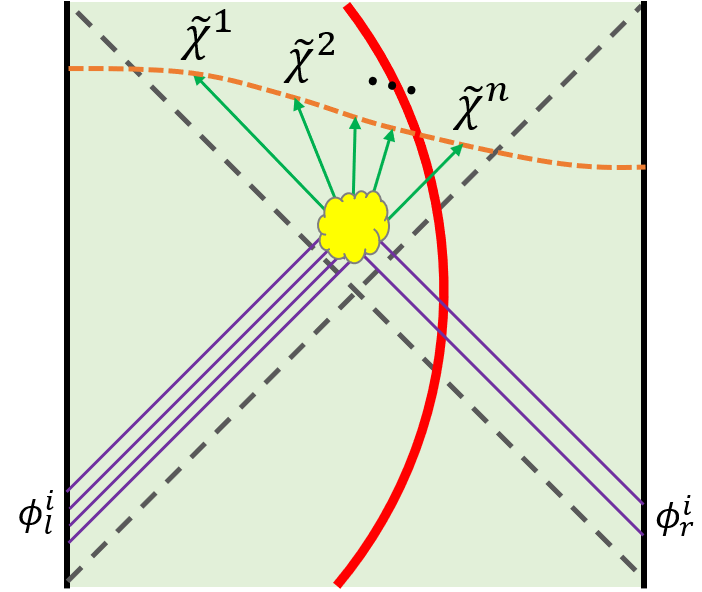
(a)

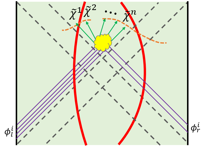
(b)

Figure 8: Measure the scattering amplitude of boundary particles behind horizon. (a) is sending one probe to measure the amplitude to outgoing particles $\{\tilde{\chi}^{1},\cdots,\tilde{\chi}^{n}\}$ on the whole Cauchy slice in thermofield double state, where $\tilde{\chi}^{j}(s)\equiv\rho^{-is}\chi^{j}\rho^{is}$ are the modular flowed bulk operators. (b) is sending two probes in a more general spacetime (say long wormholes) to measure the amplitude because the “atmosphere” of one probe can only extend to finite range. In both plots, red curves are worldlines of probe, orange dashed lines are the spatial slices (“atmosphere”) related to the probe.

There is one way to study the outgoing particles by turning on some explicit coupling between two boundaries to form a traversable wormhole after all incoming particles are injected. The traversable wormhole opens a throat for outgoing particles and they could be seen by boundary observer. This proposal was studied in Haehl:2021tft by computing six-point function in AdS₂. However, how many outgoing particles will be seen by boundary observer depends on the width of the throat opened by the traversable wormhole. Moreover, the negative energy from the explicit coupling to support the traversable wormhole will collide with the outgoing particles and thus modulates the outgoing signal with details depending on the collision process.

Alternatively, we can use our modular Hamiltonian to send the apparatus for outgoing particles into the horizon and measure the scattering amplitude without changing the geometry. We can study the following inner product

$$\mathcal{A}(\{\phi_{l}^{i},\phi_{r}^{j}\}\rightarrow\{\chi^{k}\})=\text{Tr}\left(\rho^{1-is}\chi^{1}\cdots\chi^{n}\rho^{is}\phi_{l}^{1}(t_{l1})\cdots\phi_{l}^{i}(t_{li})\phi_{r}^{1}(t_{r1})\cdots\phi_{r}^{j}(t_{rj})\right)$$ (173)

where $\{\chi^{k}\}$ is a set of bulk operators initiated on global $t=0$ slice acting on thermofield double state with the probe $\rho$. Note that the full set of $\chi^{k}$ could be reconstructed by HKLL method explained in Secrtion 3.5 by both left and right boundary data. Scanning all possible $\chi^{k}$ gives full information of the scattering amplitude of the collision among incoming particles behind horizon on a spatial slice related to the infalling probe after proper time $s\beta_{probe}/(2\pi)$. See Fig. 8a for an illustration. Because we measure the scattering behind horizon directly, this approach also has advantage of not modulating the outgoing signal comparing to the method in Haehl:2021tft .

One might suspect that modulation still occurs because incoming and outgoing particles will collide with the probe when they intersect with the worldline of the latter. However, this is a subleading effect for the collision among particles because this scattering amplitude is proportional to the energy of the probe, which is low due to its worldline being far from boundary. One can already see this from the computation in Section 3.5 that the pole location of causal correlator for $\ell>0$ does not contain Shapiro delay that one might have expected due to the collision between $\psi_{l}(t)$ with the probe before hitting $\chi_{s}$.

In more general spacetime, say long wormhole (e.g. Shenker:2013pqa ; Goel:2018ubv and also Brown:2019rox ), where we could only apply the modular flow to atmosphere operators that are close to the probe Jafferis:2020ora , we can simply generalize above approach by including multiple probes with different worldlines to detect outgoing particles at different locations using the same inner product (173) replacing $\rho$ by the reduced density matrix for multiple probes (Fig. 8b).

Appendix A Analysis of twisted boundary conditions

Given the solution of Liouville equation, we will not be able to construct a solution in which all $\sigma_{ab}$ meet at all $\mathbb{Z}\beta_{a}$ points and also respect all symmetries. First, requiring

$$\sigma_{rl}^{s}(\beta_{r},\tau)=\sigma_{rl}^{s+1}(0,\tau),\quad\sigma_{rl}^{s}(\tau,0)=\sigma_{rl}^{s+1}(\tau,\beta_{l})$$ (174)

for all $s$ is inconsistent with periodic condition $\sigma_{rl}^{k}=\sigma_{rl}^{0}$. Above condition requires the function pair choice for $\sigma_{rl}^{s}$ be $(h_{s},f)$ where the second function could be the same $f$. Also, a careful check of this ansatz leads to

$$h_{s}(\beta_{r})=h_{s+1}(0)$$ (175)

We must have $h_{s}$ and $f$ both to be monotonous function to guarantee correlation function to be real (because of $1/q$ power of $e^{\sigma}$). However, this obviously contradicts with (175) and $h_{k}=h_{0}$ because periodic function cannot be monotonous. Indeed, this argument can be generalized to the case where difference of both sides of (174) is a constant, in which (175) still holds.

There are many other inconsistencies related to $\sigma_{ll}^{s}$ and $\sigma_{rr}^{s}$. For $\sigma_{ll}^{s}$, the above periodic issue is avoid by the reflection (73). By similar argument, boundary condition

$$\sigma_{ll}^{s}(\beta_{l},\tau)=\sigma_{ll}^{s+1}(0,\tau),~{}\sigma_{ll}^{s}(\tau,0)=\sigma_{ll}^{s+1}(\tau,\beta_{l}),~{}\sigma_{ll}^{s}(\beta_{l},\tau)=\sigma_{rl}^{s}(\beta_{r},\tau),~{}\sigma_{ll}^{s}(0,\tau)=\sigma_{rl}^{s}(0,\tau)$$ (176)

requires the function choice for $\sigma_{ll}^{s}$ to be $(f_{s},f)$ where all $f_{s}$ are related by $SL(2)$ transformations. The periodic condition for $s=k$ leads to

$$(f_{k}(0),f(\tau))=(f_{0}(\tau),f(0))\implies f_{0}\simeq f$$ (177)

Hence, each $f_{s}$ is some $SL(2)$ transformation of $f$. Taking $f_{0}=\frac{a+bf}{c+df}$ into UV condition (73) leads to $f$ being in the form of $u+v\tan(\omega\tau+\gamma)$. Indeed, any $SL(2)$ of $f$ is also in this form.

Similarly, for $\sigma_{rr}^{s}$, we have

$$\sigma_{rr}^{s}(\beta_{r},\tau)=\sigma_{rr}^{s+1}(0,\tau),~{}\sigma_{rr}^{s}(\tau,0)=\sigma_{rr}^{s+1}(\tau,\beta_{r}),~{}\sigma_{rr}^{s}(\tau,\beta_{r})=\sigma_{rl}^{s}(\tau,\beta_{l}),~{}\sigma_{rr}^{s}(\tau,0)=\sigma_{rl}^{s}(\tau,0)$$ (178)

which leads to the function choice of $\sigma_{rr}^{s}$ to be $(\bar{h}_{s},h)$ where all $\bar{h}_{s}$ and $h_{s}$ are related by $SL(2)$. Moreover, the periodic condition for $s=k$ and UV condition leads to $h_{s}\simeq h$ with $h$ in the same form as $f$ but with possibly different parameters. Taking such tangent related functions, one can easily show that the last two equations of (176) (or (178)) that connect $\sigma_{rl}^{s}$ with $\sigma_{ll}^{s}$ (or $\sigma_{rr}^{s}$) on two ends cannot be satisfied.

Appendix B Solving the recurrence

There are two sequences to solve. To solve the recurrence, we first define the following new variables

$$y_{s} =\frac{\cos(\omega\beta_{l}+\gamma_{s})}{\cos\gamma_{s}},\quad x_{s}=v_{s}\sec^{2}\gamma_{s},\quad\lambda=\sin^{2}\omega\beta_{l}$$ (179)

$$\tilde{y}_{s} =\frac{\cos(\omega\beta_{r}+\tilde{\gamma}_{s})}{\cos\tilde{\gamma}_{s}},\quad\tilde{x}_{s}=\tilde{v}_{s}\sec^{2}\tilde{\gamma}_{s},\quad\tilde{\lambda}=\sin\omega\beta_{l}\sin\omega\beta_{r}$$ (180)

The recurrence (85) and (86) can be rewritten as

$$x_{s+1}=\alpha_{s}x_{s}y_{s}^{-2},\quad y_{s+1}-y_{s}=-\alpha_{s}\lambda x_{s}y_{s}^{-1}$$ (181)

and (93) and (94) can be rewritten as

$$\tilde{x}_{s+1}=\tilde{\alpha}_{s}\tilde{x}_{s}\tilde{y}_{s}^{-2},\quad\tilde{y}_{s+1}-\tilde{y}_{s}=\tilde{\alpha}_{s}\tilde{\lambda}\tilde{x}_{s}\tilde{y}_{s}^{-1}$$ (182)

It follows that

$$y_{s+1}/y_{s}-1=-\lambda x_{s+1},\quad\tilde{y}_{s+1}/\tilde{y}_{s}-1=\tilde{\lambda}\tilde{x}_{s+1}$$ (183)

Taking them back to the second equations of (181) and (182) leads to a recurrence for $y_{s}$ and $\tilde{y}_{s}$ on themselves

$$\frac{y_{s+1}/y_{s}-1}{y_{s}/y_{s-1}-1}=\alpha_{s}y_{s}^{-2},\quad\frac{\tilde{y}_{s+1}/\tilde{y}_{s}-1}{\tilde{y}_{s}/\tilde{y}_{s-1}-1}=\tilde{\alpha}_{s}\tilde{y}_{s}^{-2}$$ (184)

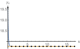
(a)

(b)

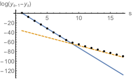
(c)

Figure 9: (a) Exact solution of $y_{s}$ versus approximation $y(s)$. (b) Exact solution of $x_{s}$ versus approximation $x(s)$. (c) Exact solution of $\log(y_{s}-y_{s-1})$ versus approximation $\log(y(s)-y(s-1))$. In all plots, the black dots are exact data, blue curve is the approximation for $s<\left\lfloor k/2\right\rfloor$ and yellow dashed curve is for $s>\left\lfloor k/2\right\rfloor$. We see that both $x_{s}$ and $y_{s}$ converge very fast and the approximations match very well. The difference between the approximations of $s<\left\lfloor k/2\right\rfloor$ and $s>\left\lfloor k/2\right\rfloor$ are very small and only visible when we check $y_{s}-y_{s-1}$ in log plot. Other parameters are $\beta_{l}=1$, $\beta_{r}=4$, $\mathcal{J}=20$, $\alpha=1/10$ and $k=17$.

However, these recurrence cannot be solved explicitly. We assume $k$ to be an odd number. Let us take large $\mu$ case in which $\alpha_{s}$ and $\tilde{\alpha}_{s}$ become identical and piecewise constant

$$\alpha_{s}=\tilde{\alpha}_{s}\rightarrow\begin{cases}\alpha=e^{-\mu(q-2)}&s=0,\cdots,\left\lfloor k/2\right\rfloor-1\\ 1&s=\left\lfloor k/2\right\rfloor\\ 1/\alpha&s=\left\lfloor k/2\right\rfloor+1,\cdots,k-1\end{cases}$$ (185)

Furthermore, we will solve (184) approximately by replacing it with its differential version

$$(\log(\log y)^{\prime})^{\prime}=\log\alpha_{s}-2\log y$$ (186)

where $y=y(s)$. This differential equation can be solved for each piece where $\alpha_{s}$ is a constant as

$$y(s)=\begin{cases}\alpha^{1/2}\exp\left[c_{1}\coth(c_{1}s+b_{1})\right]&s<\left\lfloor k/2\right\rfloor\\ \alpha^{-1/2}\exp\left[c_{2}\coth(c_{2}s+b_{2})\right]&s>\left\lfloor k/2\right\rfloor\end{cases}$$ (187)

Here we ignored the $s=\left\lfloor k/2\right\rfloor$ case because it is just one point and not related to our later analytic continuation. Here need to choose $c_{i}$ and $b_{i}$ to be real parameters because (181) shows that $y_{s}$ is monotonically decreasing sequence. To determine these four parameters, we will impose the following condtions. For small $\alpha$, we find that $y$ decays to its limit value very fast (see Fig. 9), we can use the limit value $y_{\infty}$ and initial value $y_{0}$ to fix $c_{1}$ and $b_{1}$. Here is a caveat that the limit value $y_{\infty}$ should be defined as the one using $\alpha_{s}=\alpha$ all along the sequence. But it turns out to be the same as the limit value if we use (185) and take $k$ to infinity limit, which we denote as $y_{\infty}$. To fix $c_{2}$ and $b_{2}$, besides the limit value $y_{\infty}$, we also use the continuity condition of $y(s)$ at $s=\left\lfloor k/2\right\rfloor$. One can easily solve them as

$$c_{1} =\log(y_{\infty}/\alpha^{1/2}),\quad b_{1}=\text{arccoth}(\log(y_{0}/\alpha^{1/2})/\log(y_{\infty}/\alpha^{1/2}))$$ (188)

$$c_{2} =\log(y_{\infty}\alpha^{1/2}),\quad b_{2}=\text{arccoth}\left(\frac{\log\alpha+c_{1}\coth(c_{1}\left\lfloor k/2\right\rfloor+b_{1})}{c_{2}}\right)-c_{2}\left\lfloor k/2\right\rfloor$$ (189)

The numerics in Fig. 9 show that this approximation matches with exact result pretty well. With solution (187), we can take it into the first equation of (181) and find

$$x_{s}=\begin{cases}x_{0}e^{-2c_{1}\sum_{i=0}^{s-1}\coth(c_{1}i+b_{1})}&s\leq\left\lfloor k/2\right\rfloor\\ x_{0}y(\lfloor k/2\rfloor)e^{-2c_{1}\sum_{i=0}^{\left\lfloor k/2\right\rfloor-1}\coth(c_{1}i+b_{1})-2c_{2}\sum_{i=\left\lfloor k/2\right\rfloor+1}^{s-1}\coth(c_{2}i+b_{2})}&s>\left\lfloor k/2\right\rfloor\end{cases}$$ (190)

Similarly, if we approximate the sum as integral (just like taking recurrence sequence as differential equation), we get

$$x(s)=\begin{cases}\frac{x_{0}\sinh^{2}b_{1}}{\sinh^{2}(c_{1}s+b_{1})}&s<\left\lfloor k/2\right\rfloor\\ \frac{x_{0}\sinh^{2}b_{1}\sinh^{2}(c_{2}\left\lfloor k/2\right\rfloor+b_{2})}{\sinh^{2}(c_{1}\left\lfloor k/2\right\rfloor+b_{1})\sinh^{2}(c_{2}s+b_{2})}&s>\left\lfloor k/2\right\rfloor\end{cases}$$ (191)

For our approximation (75), we will use the two solutions in (187) and (191) respectively in $\sigma_{ll}^{s}$ and $\sigma_{ll}^{k-s}$. In terms of $x(s)$ and $y(s)$, we have the large $q$ solution to be

$$g_{ll}(s) e^{\sigma_{ll}^{s}(\tau_{1},\tau_{2})/q}=\frac{1}{2}\left(\omega\lambda\mathcal{J}^{-1}x(s)^{1/2}y(s)[(\sin\omega(\beta_{l}-\tau_{1})+y(s)\sin\omega\tau_{1})\right.$$

$$\left.\times(\sin\omega\tau_{2}+y(s)\sin\omega(\beta_{l}-\tau_{2}))-\lambda x(s)\sin\omega\tau_{2}\sin\omega(\beta_{l}-\tau_{1})]^{-1}\right)^{2/q}$$ (192)

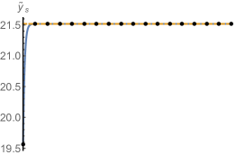
(a)

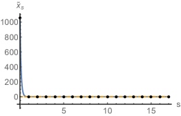
(b)

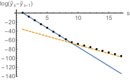
(c)

Figure 10: (a) Exact solution of $\tilde{y}_{s}$ versus approximation $\tilde{y}(s)$. (b) Exact solution of $\tilde{x}_{s}$ versus approximation $\tilde{x}(s)$. (c) Exact solution of $\log(\tilde{y}_{s}-\tilde{y}_{s-1})$ versus approximation $\log(\tilde{y}(s)-\tilde{y}(s-1))$. All settings are the same as Fig. 9.

It is very similar to solve the other recurrence sequence using the differential equation approximation. However, from the second equation in (182), $\tilde{y}_{s}$ is a monotonically increasing function. Hence, the solution to the same differential equation (186) should be chosen as

$$\tilde{y}(s)=\begin{cases}\alpha^{1/2}\exp\tilde{c}_{1}\tanh(\tilde{c}_{1}s+\tilde{b}_{1})&s<\left\lfloor k/2\right\rfloor\\ \alpha^{-1/2}\exp\tilde{c}_{2}\tanh(\tilde{c}_{2}s+\tilde{b}_{2})&s>\left\lfloor k/2\right\rfloor\end{cases}$$ (193)

where the parameters should be determined in the same way as

$$\tilde{c}_{1} =\log(\tilde{y}_{\infty}/\alpha^{1/2}),\quad\tilde{b}_{1}=\text{arctanh}(\log(\tilde{y}_{0}/\alpha^{1/2})/\log(\tilde{y}_{\infty}/\alpha^{1/2}))$$ (194)

$$\tilde{c}_{2} =\log(\tilde{y}_{\infty}\alpha^{1/2}),\quad\tilde{b}_{2}=\text{arctanh}\left(\frac{\log\alpha+\tilde{c}_{1}\tanh(\tilde{c}_{1}\left\lfloor k/2\right\rfloor+\tilde{b}_{1})}{\tilde{c}_{2}}\right)-\tilde{c}_{2}\left\lfloor k/2\right\rfloor$$ (195)

It follows that

$$\tilde{x}(s)=\begin{cases}\frac{\tilde{x}_{0}\cosh^{2}\tilde{b}_{1}}{\cosh^{2}(\tilde{c}_{1}s+\tilde{b}_{1})}&s<\left\lfloor k/2\right\rfloor\\ \frac{\tilde{x}_{0}\cosh^{2}\tilde{b}_{1}\cosh^{2}(\tilde{c}_{2}\left\lfloor k/2\right\rfloor+\tilde{b}_{2})}{\cosh^{2}(\tilde{c}_{1}\left\lfloor k/2\right\rfloor+\tilde{b}_{1})\cosh^{2}(\tilde{c}_{2}s+\tilde{b}_{2})}&s>\left\lfloor k/2\right\rfloor\end{cases}$$ (196)

From Fig. 10, we see clearly that our approximation works very well. By our solution of $s=0$, we have

$$x_{0} =\tilde{x}_{0}=\sec^{2}\omega(\beta_{l}+\beta_{r})/2$$ (197)

$$y_{0} =\tilde{y}_{0}=\cos\omega(\beta_{l}-\beta_{r})/2\sec\omega(\beta_{l}+\beta_{r})/2$$ (198)

In terms of $\tilde{x}(s)$ and $\tilde{y}(s)$, we have

$$g_{rl}(s) e^{\sigma_{rl}^{s}(\tau_{1},\tau_{2})/q}=\frac{\text{sgn}(g_{rl}(s))}{2}\left(\omega\tilde{\lambda}\mathcal{J}^{-1}\tilde{x}(s)^{1/2}\tilde{y}(s)[(\sin\omega(\beta_{r}-\tau_{1})+\tilde{y}(s)\sin\omega\tau_{1})\right.$$

$$\left.\times(\sin\omega\tau_{2}+\tilde{y}(s)\sin\omega(\beta_{l}-\tau_{2}))+\tilde{\lambda}\tilde{x}(s)\sin\omega\tau_{2}\sin\omega(\beta_{r}-\tau_{1})]^{-1}\right)^{2/q}$$ (199)

For $\sigma_{rr}^{s}$ and $\sigma_{lr}^{s}$, we can simply switch $\beta_{l}\leftrightarrow\beta_{r}$. Note that to get $\sigma_{lr}^{s}$, we can also use symmetry (68), which turns out to be the same as swap $\beta_{l}\leftrightarrow\beta_{r}$. This is a consistent check that based on the fact that $\tilde{x}_{s}$ and $\tilde{y}_{s}$ are both invariant under swap $\beta_{l}\leftrightarrow\beta_{r}$, which is because initial values $\tilde{x}_{0}$ and $\tilde{y}_{0}$ and recurrence equations all preserve this symmetry.

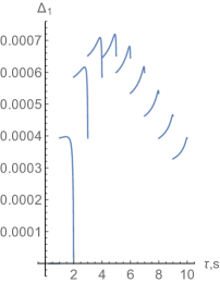
(a)

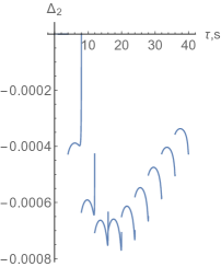
(b)

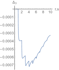
(c)

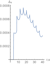
(d)

Figure 11: The errors of twist boundary condition. The horizontal axis is $\tau$ plotted over $[0,\beta_{l}]$ for $\Delta_{1,3}$ and over $[0,\beta_{r}]$ for $\Delta_{2,4}$ for all $s$ in order, that is, putting all different $s$ in one plot where $[0,\beta_{a}]$ is for $s=0$, $[\beta_{a},2\beta_{a}]$ is for $s=1$ and so on. Here the parameters are $\beta_{l}=1$, $\beta_{r}=4$, $\mathcal{J}=20$, $\alpha=1/500$, $q=20$ and $k=9$. If we increase $\beta$, namely decrease $\alpha$, the error will overall be smaller. We see that the error is much smaller than $1/q=0.05$ for this choice of small $\alpha$.

Given this solution, we need to check how much the twist boundary condition in (63)-(66) are violated. Note that in large $\beta$ limit, the factors involving hyperbolic functions become

$$\left|\frac{\sinh\mu\sinh\frac{(k-2(s-1))\mu}{2}}{\cosh\frac{(k-2s)\mu}{2}}\right| \approx\left|\frac{\sinh\mu\cosh\frac{(k-2(s-1))\mu}{2}}{\sinh\frac{(k-2s)\mu}{2}}\right|\rightarrow\begin{cases}\frac{1}{2}e^{2\mu}&s\leq\left\lfloor k/2\right\rfloor\\ \frac{1}{2}e^{\mu}&s=\left\lfloor k/2\right\rfloor+1\\ \frac{1}{2}&s>\left\lfloor k/2\right\rfloor+1\end{cases}$$ (200)

$$\left|\frac{\sinh\mu\sinh\frac{(k-2s)\mu}{2}}{\cosh\frac{(k-2(s-1))\mu}{2}}\right| \approx\left|\frac{\sinh\mu\cosh\frac{(k-2s)\mu}{2}}{\sinh\frac{(k-2(s-1))\mu}{2}}\right|\rightarrow\begin{cases}\frac{1}{2}&s\leq\left\lfloor k/2\right\rfloor\\ \frac{1}{2}e^{\mu}&s=\left\lfloor k/2\right\rfloor+1\\ \frac{1}{2}e^{2\mu}&s>\left\lfloor k/2\right\rfloor+1\end{cases}$$ (201)

All LHS of (63)-(66) are zero by our ansatz. RHS are generally nonzero and can be categorized into four types

$$\Delta_{1} =e^{2\mu}(\exp(\sigma_{ll}^{s}(\beta_{l},\tau)/q)-\exp(\sigma_{rl}^{s}(\beta_{r},\tau)/q))$$ (202)

$$\Delta_{2} =e^{2\mu}(\exp(\sigma_{lr}^{s}(\beta_{l},\tau)/q)-\exp(\sigma_{rr}^{s}(\beta_{r},\tau)/q))$$ (203)

$$\Delta_{3} =e^{2\mu}(\exp(\sigma_{lr}^{s}(\tau,0)/q)-\exp(\sigma_{ll}^{s}(\tau,0)/q))$$ (204)

$$\Delta_{4} =e^{2\mu}(\exp(\sigma_{rr}^{s}(\tau,0)/q)-\exp(\sigma_{rl}^{s}(\tau,0)/q))$$ (205)

which are upper bound of errors in RHS. In Fig. 11, we plot $\Delta_{i}$ for all choices of $\tau$ and $s$. In this figure, we find that when we increase $\beta$, equivalently decrease $\alpha$, the errors decrease. With the parameters Fig. 11, we see that the errors are typically much smaller than $1/q$. Therefore, we should trust our solution in large $\beta$ limit.

Appendix C Validity of large $q$ solution

Although we find perfect match between our large $q$ solution with bulk semiclassical computation, we should not expect the solution well describing black hole physics for arbitrary large $s$. On one hand, SYK model has distinct long time behavior than semiclassical gravity, e.g. ramp and plateau in the form factor Saad:2018bqo are described non-pertrubative effects in JT gravity. On the other hand, for a black hole, the probe will not extend its worldline inside horizon for infinite proper time because it will eventually hit singularity. However, it seems neither of these two bounds can be applied our current analysis. The first type of long time behavior is for boundary time. It is unclear how that will be related to the proper time of an infalling probe behind horizon. In particular, from Fig. 3a and Fig. 3b, it is clear that after just order one proper time evolution, the spatial slice of probe already goes beyond two Rindler wedges. The second type of limitation from singularity unfortunately does not exist in JT gravity because it has constant curvature everywhere. One could define the singularity of JT gravity as the curve with large and negative dilaton value $-\phi_{0}$ understood as dimensional reduction from higher dimensional near extremal black hole Harlow:2018tqv . However, for large $\phi_{0}$, the singularity is time-like and most probes are free from hitting it. It was argued in Jafferis:2020ora that the modular flow formula should hold up to scrambling time order of proper time. This seems to be the only bound for $s$. This bound is quite high and grants our solution to see the regions way behond horizon.

Besides $s$, we still need to check in more details on how other parameters are bounded for the validity of the large $q$ solution. These bounds mainly come from the limitation of various approximations we take in the solution. The first approximation is taking the correlation function in thermofield double state for $\sigma_{ab}^{0}$ in (76) and (77) when $\mu$ is large. To estimate the error, we need to use the following identity

$$e^{-\beta V} \propto\prod_{j=1}^{N}(1-2i\psi_{l}^{j}\psi_{r}^{j}\tanh\frac{\mu}{2})\propto\prod_{j=1}^{N}\left[\left|0_{j}\right\rangle\left\langle 0_{j}\right|+2e^{-\mu}\psi_{l}^{j}\left|0_{j}\right\rangle\left\langle 0_{j}\right|\psi_{l}^{j}\right]$$

$$\approx\left|0\right\rangle\left\langle 0\right|+e^{-\mu}\sum_{j=1}^{N}2\psi_{l}^{j}\left|0\right\rangle\left\langle 0\right|\psi_{l}^{j}$$ (206)

where we used $\left|0_{j}\right\rangle\left\langle 0_{j}\right|=(1-2i\psi_{l}^{j}\psi_{r}^{j})$ up to normalization and assumed $e^{-\mu}\ll 1$. Taking this into $s=0$ correlation function (here we suppress the average over indices for simplicity)

$$\hat{g}(\tau_{1},\tau_{2})=\frac{\text{Tr}\rho^{k}\psi_{a}(\tau_{1})\psi_{b}(\tau_{2})}{\text{Tr}\rho^{k}}\approx\hat{g}_{\text{tfd}}(\tau_{1},\tau_{2})\left(1+\frac{e^{-\mu k}\xi^{k}\mathcal{F}(\tau_{1},\tau_{2})}{1+Ne^{-\mu k}\xi^{k}}\right)+\text{subleading}$$ (207)

where

$$\xi \equiv\frac{2}{N}\sum_{j}\frac{\left\langle 0|\psi_{l}^{j}e^{-\beta_{l}H_{l}-\beta_{r}H_{r}}\psi_{l}^{j}|0\right\rangle}{Z_{\beta}}\sim O(1),\quad Z_{\beta}\equiv\left\langle 0|e^{-\beta_{l}H_{l}-\beta_{r}H_{r}}|0\right\rangle=\text{Tr}_{\mathcal{H}_{l}}e^{-\beta H_{l}}$$ (208)

$$\mathcal{F}(\tau_{1},\tau_{2}) \equiv N\left[\frac{\left\langle 0|\psi_{l}^{j}e^{-\beta_{l}H_{l}/2-\beta_{r}H_{r}/2}\psi_{a}(\tau_{1})\psi_{b}(\tau_{2})e^{-\beta_{l}H_{l}/2-\beta_{r}H_{r}/2}\psi_{l}^{j}|0\right\rangle}{\xi\left\langle 0|e^{-\beta H_{l}/2}\psi_{a}(\tau_{1})\psi_{b}(\tau_{2})e^{-\beta H_{l}/2}|0\right\rangle}-1\right]\sim O(1)$$ (209)

To derive this, we used large $N$ factorization and $SO(N)$ symmetry of correlators. To gurantee our thermofield double approximation works for all $k\geq 1$, we need to impose

$$e^{-\mu}/N\ll 1$$ (210)

which is obviously satisfied given $e^{-\mu}\ll 1$.

The second approximation is assuming $\sigma_{ab}^{s}$ continuous and checking if errors $\Delta_{i}\ll 1/q$. All four $\Delta_{i}$ are in the same order, and let us check $\Delta_{1}$ as an example. In large $\mathcal{J}$ limit, we can use (116) to show that $\tilde{y}_{s}\gg 1$ (unless $\delta_{l}$ is too close to 0 or $\pi$). Similarly, we can use recurrence to show that $y_{0}=\tilde{y}_{0}\gg 1$, $y_{1}\approx y_{0}(1-\alpha)$, $y_{k}\approx y_{k-1}(1-O(\alpha(\alpha y_{0}^{-2})^{s-1}))$ and $\tilde{y}_{s}-y_{s}\sim y_{0}\alpha$ for $s\geq 1$. Besides, $x_{s}$ has same scaling as $\tilde{x}_{s}$ in (117) and their difference is $x_{s}-\tilde{x}_{s}\sim O(\alpha^{2}(\alpha\tilde{y}_{0}^{-2})^{s-1})$ for $s\geq 2$ (and is zero for $s=0,1$). Then, we have

$$\Delta_{1} \approx e^{2\mu}\left[\left(\frac{\omega\sin\pi\delta_{l}x(s)^{1/2}/\mathcal{J}}{\sin\omega\tau+y(s)\sin\omega(\beta_{l}-\tau)}\right)^{2/q}-\left(\frac{\omega\sin\pi\delta_{l}\tilde{x}(s)^{1/2}/\mathcal{J}}{\sin\omega\tau+\tilde{y}(s)\sin\omega(\beta_{l}-\tau)}\right)^{2/q}\right]$$

$$\lesssim e^{2\mu}\left(\frac{\alpha^{1/2}(\alpha y_{0}^{-2})^{\frac{s-1}{2}}}{(\beta\mathcal{J})^{2}}\right)^{2/q}\frac{\alpha}{q}$$

$$\lesssim\frac{1}{q}e^{-\mu q}(\beta\mathcal{J})^{-4/q}$$ (211)

where we assume $\sin\omega\tau\sim\sin\omega(\beta_{l}-\tau)\sim O(1)$ and in the last line we take $s=1$ to get the upper bound. To guarantee it being smaller than $1/q$, we need to impose

$$e^{-\mu q}(\beta\mathcal{J})^{-4/q}\ll 1$$ (212)

The third approximation is replacing the recurrence sequence with differential equation. This approximation causes errors for $x_{s}$ and $y_{s}$ (and their tilde version). This error should be smaller than $x_{s}-\tilde{x}_{s}$ and $y_{s}-\tilde{y}_{s}$. As (211) could also be understood as counting for the error of latter type, we shoul validate this approximation under condition (212).

The last approximation is using the sum over image as the solution to Schwinger-Dyson equation. This error is exponentially small for $s$ not close to $\left\lfloor k/2\right\rfloor$ as indicated in Fig. 5. For $s$ close to $\left\lfloor k/2\right\rfloor$, the image and correlator itself are both exponentially small, there could exist $O(1)$ relative error though the absolute error is still exponentially small. It is not easy to analyze the error precisely there because we do not have a full solution to Schwinger-Dyson equation. However, we could understand this error as putting some restriction on our analytic continuation of $s$. In other words, we should require $\Im W_{2}\ll\Im W_{1}$ in (114) for some range of $s$. In large $\mathcal{J}$ limit, we have

$$\tilde{c}_{2}\approx\log\frac{\beta\mathcal{J}\alpha^{1/2}}{\pi}\sin\pi\delta_{l},\quad\tilde{b}_{2}\approx\frac{1}{2}\log(\tilde{c}_{2}/\alpha)$$ (213)

Here we see a competition between $\beta\mathcal{J}$ and $\alpha$ in $\tilde{c}_{2}$ and $\tilde{b}_{2}$ will have $\pm i\pi/2$ imaginary part if $\tilde{c}_{2}<0$. Nevertheless, we could require $|\Re(\tilde{c}_{2}+\tilde{b}_{2})|\gg 0$ for simplicity. This leads to

$$|\log\beta\mathcal{J}+\frac{1}{2}\Re\log\tilde{c}_{2}|\gg 0\implies\begin{cases}\alpha^{1/2}\beta\mathcal{J}\gg\exp(\beta^{-2}\mathcal{J}^{-2})\text{ or }\alpha^{1/2}\beta\mathcal{J}\ll\exp(-\beta^{-2}\mathcal{J}^{-2})&\text{(a)}\\ \left|\frac{\beta\mathcal{J}\alpha^{1/2}}{\pi}\sin\pi\delta_{l}-1\right|\ll\beta^{-2}\mathcal{J}^{-2}&\text{(b)}\end{cases}$$ (214)

where case (a) means overwhelming large $\beta\mathcal{J}$ or $1/\alpha$ leads to large $|\tilde{c}_{2}|$, and case (b) means $\tilde{c}_{2}$ is very close to zero. For case (a), $\tilde{y}(1-is)$ is again small oscillating function around its average value $\tilde{y}(1)$. Using a similar approximation towards (119), we have

$$W_{2}(s,t)\approx\left(\frac{(2\pi\sin\pi\delta_{l}/2)/(\beta\mathcal{J})}{Y(s)\sin\omega(\beta_{l}/2+it)+Y(s)^{-1}\sin\omega(\beta_{l}/2-it)}\right)^{2/q}$$ (215)

where

$$Y(s)=\frac{(1+\alpha)(\cosh(\tilde{c}_{2}+\tilde{b}_{2})\cos\tilde{c}_{1}s+i\sinh(\tilde{c}_{2}+\tilde{b}_{2})\sin\tilde{c}_{1}s)}{\cosh\tilde{b}_{2}}$$ (216)

As $|\tilde{c}_{2}|$ is very large, this leads to

$$|Y(s)|\sim e^{|\tilde{c}_{2}|}\implies|W_{2}/W_{1}|\sim e^{-2|\tilde{c}_{2}|/q}$$ (217)

For small image contribution, we need

$$(\beta\mathcal{J}\alpha^{1/2})^{\mp 2/q}\ll 1$$ (218)

where minus sign is for $\beta\mathcal{J}\alpha^{1/2}\gg 1$ and plus sign is for $\beta\mathcal{J}\alpha^{1/2}\ll 1$. For case (b), we have $\tilde{y}(1-is)\approx 1$ and $\tilde{x}(1-is)\approx\tilde{x}_{0}$ for all $s\ll 1/|\tilde{c}_{2}|\rightarrow\infty$, this leads to

$$W_{2}(s,t)\sim 1/x_{0}^{2/q}\sim(\beta^{2}\mathcal{J}^{2})^{-2/q}\implies|W_{2}/W_{1}|\sim(\beta\mathcal{J})^{-2/q}$$ (219)

For small image contribution, we need

$$(\beta\mathcal{J})^{-2/q}\ll 1$$ (220)

Summarizing above analysis, we should expect our solution valid generally for $e^{-\mu}\ll 1$ and $(\beta\mathcal{J})^{-1/q}\ll 1$. If the $e^{-\mu q/2}$ and $1/\beta\mathcal{J}$ are two distinct scales, we require the distinct large enough as (218). Otherwise, we require them to be in very close scales as $\beta\mathcal{J}e^{-\mu q/2}\rightarrow\pi/\sin\pi\delta_{l}$. For the case we are mostly interested in, we can first take large $\mu$ limit and then take large $\beta\mathcal{J}$, which is in validity of our solution.

Appendix D Euclidean wormhole $SL(2,R)$ charge from large $q$ SYK solution

The essence of $M$ in gravitational computation is the magnitude of $SL(2,R)$ charge carried by insertion of $\rho_{0}$. Therefore, we should first find a way to define $SL(2,R)$ charge for a given solution (59) on the “necklace” diagram. In the following, we will only focus on $\sigma_{rl}^{s}$, whose solution is copied here

$$e^{\sigma_{rl}^{s}(\tau_{1},\tau_{2})}=\frac{h_{s}^{\prime}(\tau_{1})f^{\prime}(\tau_{2})}{\mathcal{J}\tilde{\mathcal{J}}_{s}(1-h_{s}(\tau_{1})f(\tau_{2}))^{2}}$$ (221)

Let us first forget about all conditions that we impose to fix these functions as in Section 3.3. After fixing $f$, we could restrict ourselves to the subspace of solutions to Liouville equation in which all $h_{s}$ are related to each other by an $SL(2,R)$ transformation. This subspace is isomorphic to the group manifold of $SL(2,R)$. In this sense, our solution for each $s$ given in Section 3.3 is a point in this subpace. Finding a quantity to characterize the effect of insertion $\rho_{0}$ is equivalent to measuring the “distance” between $s$-th and $(s+1)$-th points.

Such “distance” has a natural constraint that if the translation $\tau_{1}\rightarrow\tau_{1}+c$ for a constant $c$ is an $SL(2,R)$ transformation of $h_{s}$, we should count it as no “distance” away from original solution. This corresponds to the $SL(2,R)$ charge defined in (138) for circular boundary particle trjectory in EAdS₂ being invariant under translation in $\theta$. In other words, we are counting the effect of $\rho_{0}$ relative to the time translation generated by SYK Hamiltonian.

The $PSL(2,R)$ group has a 3-dimensional faithful representation by acting $SL(2,R)$ on its $sl(2,R)$ algebra by conjugation, where for a given $SL(2,R)$ transformation

$$h_{s}\rightarrow\frac{ah_{s}+b}{ch_{s}+d},\quad ad-bc=1$$ (222)

we represent it as

$$Q\equiv\begin{pmatrix}V_{0}&V_{+}\\ V_{-}&-V_{0}\end{pmatrix}\rightarrow\begin{pmatrix}a&b\\ c&d\end{pmatrix}\begin{pmatrix}V_{0}&V_{+}\\ V_{-}&-V_{0}\end{pmatrix}\begin{pmatrix}a&b\\ c&d\end{pmatrix}^{-1},\quad V_{\pm,0}\in\mathbb{R}$$ (223)

where $V_{0,\pm}$ parameterize the representation space. Indeed, our transformations of solution from $s$ to $s+1$ are all in the subgroup $PSL(2,R)$ because we will keep the direction of time unflipped. As $Q$ are elements of the representation space, it is natural to define it as the charge for each solution and use it to measure “distance”. For any two charges $Q_{1}$ and $Q_{2}$, the inner product is defined as

$$(Q_{1},Q_{2})\equiv\text{Tr}Q_{1}Q_{2}$$ (224)

and the norm of $Q_{1}-Q_{2}$ is their “distance”. This “distance” coincides with the charge of $\rho_{0}$ (namely $M$) if $Q_{1,2}$ are charges of $s$-th and $(s+1)$-th solution respectively assuming charge conservation.

For $s=0$, we have $h_{0}(\tau)=\tan\omega(\tau+\tilde{\gamma}_{0})$, whose time translation acts as

$$h_{0}(\tau+\tau_{0})=\frac{\cos\omega\tau_{0}h_{0}(\tau)+\sin\omega\tau_{0}}{-\sin\omega\tau_{0}h_{0}(\tau)+\cos\omega\tau_{0}}$$ (225)

Invariance of $Q=Q_{0}$ under this $SL(2,R)$ transformation solves $V_{0,\pm}$ in (223) as

$$Q_{0}:\quad V_{0}=0,\quad V_{+}=-V_{-}=\kappa/\beta$$ (226)

Here $1/\beta$ is due to dimensional analysis that $Q_{0}$ should match with mass $M$. $\kappa$ is an order one number that does not depend on $\mu$. This is important because $s=0$ solution should not know anything about $\rho_{0}$. Starting with $Q_{0}$, we can represent the space of $PSL(2,R)/U(1)$ by conjugation (223) of $Q_{0}$, where $U(1)$ counts for the constraint from the time translation as we proposed above.

Moving to a finite $s$ solution leads to $SL(2,R)$ matrix

$$R_{s}=\begin{pmatrix}\tilde{v}_{s}-\tilde{u}_{s}\tan\tilde{\gamma}_{s0}&\tilde{u}_{s}+\tilde{v}_{s}\tan\tilde{\gamma}_{s0}\\ -\tan\tilde{\gamma}_{s0}&1\end{pmatrix}\frac{\cos\tilde{\gamma}_{s0}}{\sqrt{\tilde{v}_{s}}}$$ (227)

where $\tilde{\gamma}_{s0}\equiv\tilde{\gamma}_{s}-\tilde{\gamma}_{0}$ and which conjugating $Q_{0}$ leads to

$$Q_{s}=\kappa/\beta\begin{pmatrix}-\tilde{u}_{s}/\tilde{v}_{s}&\tilde{u}_{s}^{2}/\tilde{v}_{s}+\tilde{v}_{s}\\ -1/\tilde{v}_{s}&\tilde{u}_{s}/\tilde{v}_{s}\end{pmatrix}$$ (228)

Using (95) and (180), we can write $Q_{s}$ in terms of $\tilde{x}_{s}$ and $\tilde{y}_{s}$. Further using recurrence (182), we can represent $Q_{s}$ in terms of $\tilde{x}_{s-1}$ and $\tilde{y}_{s-1}$. The norm square of $Q_{s+1}-Q_{s}$ is

$$M_{s}^{2}= \text{Tr}(Q_{s+1}-Q_{s})(Q_{s+1}-Q_{s})$$

$$= \frac{2\kappa^{2}}{\alpha\beta^{2}\tilde{y}_{s}^{2}}\left[2\alpha\tilde{x}_{s}\left(\alpha+\tilde{y}_{s}^{2}\right)\sin\text{$\omega\beta_{l}$}\csc\text{$\omega\beta_{r}$}+\left(\alpha^{2}+\tilde{y}_{s}^{4}+(\alpha(\alpha+4)+1)\tilde{y}_{s}^{2}\right)\csc^{2}\text{$\omega\beta_{r}$}\right.$$

$$\left.+\alpha\left(\alpha\tilde{x}_{s}^{2}\sin^{2}\text{$\omega\beta_{l}$}-4\tilde{y}_{s}^{2}\right)-2(\alpha+1)\tilde{y}_{s}\cot\text{$\omega\beta_{r}$}\left(\alpha\tilde{x}_{s}\sin\text{$\omega\beta_{l}$}+\left(\alpha+\tilde{y}_{s}^{2}\right)\csc\text{$\omega\beta_{r}$}\right)\right]$$ (229)

where we take large $\mu$ to set all $\alpha_{s}$ equal to $\alpha$. One can easily show that this is indeed an exact identity of recurrence (182) if we set $\alpha_{s}=\alpha$, which means $M_{s}^{2}$ is a constant for all $s$. This exactly corresponds to the gravitational computation in Section 4.2 where the magnitude of $SL(2,R)$ charges of all $\rho_{0}$ insertion are the same and the $SL(2,R)$ transformation of boundary circular trajectory is just power of $B(x,y)$. In particular, taking $s=0$ leads to

$$M_{s}^{2}=M_{0}^{2}=\frac{2\kappa^{2}}{\beta^{2}}\left(\frac{(1+\alpha)^{2}}{\alpha\cos^{2}\frac{\omega\beta}{2}}-4\right)\rightarrow\frac{2\kappa^{2}\mathcal{J}^{2}}{\pi^{2}\alpha}$$ (230)

where in the last step we take large $\beta\mathcal{J}$ and small $\alpha$. This corresponds to the norm of charge carried by $\rho_{0}$. To match with (159), we simply choose $\kappa=\pi/\sqrt{2}$.

Another immediate application of recurrence identity is to compute $\tilde{y}_{\infty}$. Given $\tilde{x}_{\infty}=0$, using (230) for $s\rightarrow\infty$ leads to

$$\tilde{y}_{\infty}= \frac{1}{4}\sec\omega\beta/2\Big{[}2(\alpha+1)\cos\omega(\beta_{l}-\beta_{r})/2$$

$$+\sqrt{2\left((\alpha-1)^{2}+(\alpha+1)^{2}\cos\omega(\beta_{l}-\beta_{r})-4\alpha\cos\omega\beta\right)}\Big{]}$$ (231)

Expanding in small $\alpha$ and large $\beta\mathcal{J}$ limit, we see at leading order

$$\tilde{y}_{\infty}\approx\tilde{y}_{0}(1+\alpha)\approx\tilde{y}_{1}$$ (232)

which verifies our approximation (116). Using similar method, we can find another recurrence identity for $x_{s}$ and $y_{s}$, from which we can derive

$$y_{\infty}= \frac{1}{2}\sec\omega\beta/2\left[\cos\left(\frac{\omega(\beta_{l}-\beta_{r})}{2}\right)+\alpha\cos\left(\frac{\omega(3\beta_{l}+\beta_{r})}{2}\right)\right.$$

$$\left.+\sqrt{(1-\alpha)^{2}-\left(\sin\left(\frac{\omega(\beta_{l}-\beta_{r})}{2}\right)+\alpha\sin\left(\frac{\omega(3\beta_{l}+\beta_{r})}{2}\right)\right)^{2}}\right]$$ (233)

Appendix E Bulk phase transition in large $q$ SYK

There is a very simple estimation for the bulk phase transition by changing parameter $\mu$ in large $q$ SYK model. For disconnected phase, the correlation function between SYK_l and SYK_r scales as $N^{-(q-1)}$ because it can only be built by classical correlation of random coupling $J$ between left and right Kourkoulou:2017zaj . It follows that the contribution from insertion of probe scales as $\mu N\left\langle\psi_{l}\psi_{r}\right\rangle\sim\mu N^{-(q-2)}$ which vanishes in large $N$ limit (for $q>2$). At nonlinear orders, the insertion of probe contribute by the correlations within each SYK system. Nevertheless, we can treat the partition function of $k$ replica as product of the partition function of two SYK models with inverse temperature $k\beta_{l}$ and $k\beta_{r}$ respectively plus $\mu^{2}$ and higher order perturbation.

For each SYK model with temperature $\beta$, the large $q$ effective action is derived in Choi:2020tdj

$$S_{\text{eff}}=\frac{N}{4q^{2}}\int d\tau_{1}d\tau_{2}\left[\frac{1}{4}\partial_{1}\sigma(\tau_{1},\tau_{2})\partial_{2}\sigma(\tau_{1},\tau_{2})-\mathcal{J}^{2}e^{\sigma(\tau_{1},\tau_{2})}\right]$$ (234)

where the correlation function is in the form of $G(\tau_{1},\tau_{2})=\frac{1}{2}\text{sgn}(\tau_{12})e^{\sigma(\tau_{1},\tau_{2})/q}$. The equation of motion of (234) is Liouville equation and its equilibrium solution is

$$e^{\sigma(\tau_{1},\tau_{2})}=\frac{\omega^{2}}{\mathcal{J}^{2}\cos^{2}\omega(|\tau_{12}|-k\beta/2)}$$ (235)

where $\omega$ is defined by $\omega=\mathcal{J}\cos k\beta/2$. Taking this solution back to (234), we get the on-shell action of disconnected phase to be Sarosi:2017ykf

$$S_{\text{eff}}(k\beta) =\frac{N}{2q^{2}}\int_{\tau_{1}>\tau_{2}}d\tau_{1}d\tau_{2}\omega^{2}(1-2\sec^{2}(\omega\tau_{12}-\omega k\beta/2))$$

$$=\frac{N}{4q^{2}}k\beta\omega\left(k\beta\omega-4\tan\frac{\omega k\beta}{2}\right)\rightarrow-N\frac{k\beta\mathcal{J}}{q^{2}}$$ (236)

where in the last step we take large $\beta$ limit for simplicity. To count for the correct partition function, we also need to include a constant extremal entropy $S_{0}=-\frac{N}{2}\log 2$. This can be seen from high temperature limit $\beta\rightarrow 0$ where partition function should count the total dimension of Hilbert space. For two SYK models, the total partition function is

$$Z_{disconn.}(k\beta_{l},k\beta_{r})\approx e^{-2S_{0}-S_{\text{eff}}(k\beta)},~{}\beta\equiv\beta_{l}+\beta_{r}$$ (237)

The $\mu$ dependence at quadratic order is derived from expanding $\rho_{0}$ as

$$\rho_{0}=\cosh^{N}\frac{\mu}{2}\prod_{j=1}^{N}\left(1-2i\psi^{j}_{l}\psi^{j}_{r}\tanh\frac{\mu}{2}\right)$$ (238)

and contracting $k$ insertions of $1-2i\psi^{j}_{l}\psi^{j}_{r}\tanh\frac{\mu}{2}$ within each SYK model respectively for each $j$. Given insertions are located at equal spacing of $\beta_{l,r}$ on the thermal circle of circumstance $k\beta_{l,r}$, we just need to consider the nearest contractions in large $\beta$ limit. Due to $SO(N)$ symmetry and assuming large $N$ factorization, we can derive the following contribution to on-shell action from the nearest contractions

$$e^{-\delta S_{\text{eff}}/N}=\left(\frac{1-\sqrt{1+4x}}{2}\right)^{k}+\left(\frac{1+\sqrt{1+4x}}{2}\right)^{k},~{}~{}x\equiv 4\tanh^{2}\frac{\mu}{2}G_{l}(\beta_{l})G_{r}(\beta_{r})$$ (239)

where $G_{a}(\beta_{a})=\left\langle\psi_{a}(\beta_{a})\psi_{a}\right\rangle_{k\beta_{a}}\in[0,1/2]$ are correlation functions of Majorana fermions with $\beta_{a}$ spacing on the thermal circle with circumstance of $k\beta_{a}$. Note that $x\in[0,1]$ for $\mu\in\mathbb{R}$ and exponentially suppressed in large $\beta_{l,r}$ limit. It turns out that $\delta S_{\text{eff}}$ decreases monotonically until a finite value for increasing $\mu$.

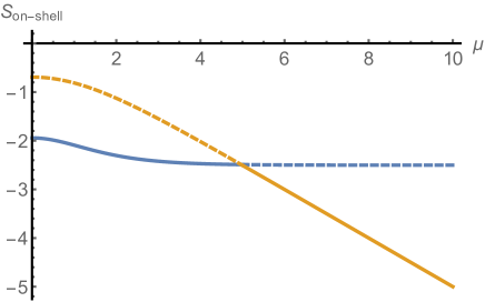
Figure 12: The comparison of on-shell action between disconnected phase (blue) and connected phase (yellow) as we increase $\mu$. At some finite $\mu=\mu_{cr}$, the dominant phase changes from the disconnected to the connected. The numbers in this plot are just for illustrative purpose.

On the other hand, for connected phase where $\mu$ is large, we can roughly ignore all SYK contributions but only keep the one coming from insertion of probe. This is equivalent to evaluating

$$Z_{conn.}(k)\approx\text{Tr}\prod_{j=1}^{N}\exp\left(-i\mu k\psi_{l}^{j}\psi_{r}^{j}\right)=\left(2\cosh\frac{\mu k}{2}\right)^{N}\approx e^{-N(-\mu k/2)}$$ (240)

where in the last step we take large $\mu$ limit. We can regard $-\mu k/2$ as the on-shell action for connected phase. It is important that this action does not include a constant extremal entropy term. Indeed, from JT gravity point of view, this reflects the fact that disconnected and connected phase have different contributions of topological term proportional to $S_{0}$. It is clear that when $-\mu kN/2>2S_{0}+S_{\text{eff}}(k\beta)+\delta S_{\text{eff}}$, the dominant phase will be disconnected and vice versa. If we ignore $\delta S$, the critical value of $\mu$ for phase transition is $\mu_{cr}\sim 2\beta\mathcal{J}/q^{2}$ in large $\beta\mathcal{J}$ limit. See Fig. 12 for an illustration. In this paper, we basically consider the regime $\mu>\mu_{cr}$ such that connected phase dominates.

References

- (1) D.L. Jafferis and L. Lamprou, Inside the Hologram: Reconstructing the bulk observer’s experience, 2009.04476.
- (2) B. Yoshida, Firewalls vs. Scrambling, JHEP 10 (2019) 132 [1902.09763].
- (3) B. Yoshida, Observer-dependent black hole interior from operator collision, Phys. Rev. D 103 (2021) 046004 [1910.11346].
- (4) J. de Boer, D.L. Jafferis and L. Lamprou, Inside holographic black holes: Melting the frozen vacuum, to appear.
- (5) S. Sachdev, Holographic metals and the fractionalized Fermi liquid, Phys. Rev. Lett. 105 (2010) 151602 [1006.3794].
- (6) S. Sachdev and J. Ye, Gapless spin-fluid ground state in a random quantum heisenberg magnet, Physical Review Letters 70 (1993) 3339.
- (7) A. Kitaev, A simple model of quantum holography, in KITP strings seminar and Entanglement, vol. 12, 2015.
- (8) J. Maldacena and D. Stanford, Remarks on the Sachdev-Ye-Kitaev model, Phys. Rev. D 94 (2016) 106002 [1604.07818].
- (9) D. Stanford, More quantum noise from wormholes, 2008.08570.
- (10) J. Maldacena and L. Susskind, Cool horizons for entangled black holes, Fortsch. Phys. 61 (2013) 781 [1306.0533].
- (11) J. Maldacena, D. Stanford and Z. Yang, Diving into traversable wormholes, Fortsch. Phys. 65 (2017) 1700034 [1704.05333].
- (12) D.A. Roberts, D. Stanford and A. Streicher, Operator growth in the SYK model, JHEP 06 (2018) 122 [1802.02633].
- (13) X.-L. Qi and A. Streicher, Quantum Epidemiology: Operator Growth, Thermal Effects, and SYK, JHEP 08 (2019) 012 [1810.11958].
- (14) S. Nezami, H.W. Lin, A.R. Brown, H. Gharibyan, S. Leichenauer, G. Salton et al., Quantum Gravity in the Lab: Teleportation by Size and Traversable Wormholes, Part II, 2102.01064.
- (15) F.M. Haehl and Y. Zhao, Size and momentum of an infalling particle in the black hole interior, JHEP 06 (2021) 056 [2102.05697].
- (16) S.-K. Jian, B. Swingle and Z.-Y. Xian, Complexity growth of operators in the SYK model and in JT gravity, JHEP 03 (2021) 014 [2008.12274].
- (17) Y.D. Lensky, X.-L. Qi and P. Zhang, Size of bulk fermions in the SYK model, JHEP 10 (2020) 053 [2002.01961].
- (18) P. Gao and D.L. Jafferis, A traversable wormhole teleportation protocol in the SYK model, JHEP 07 (2021) 097 [1911.07416].
- (19) A. Lucas, Operator size at finite temperature and Planckian bounds on quantum dynamics, Phys. Rev. Lett. 122 (2019) 216601 [1809.07769].
- (20) T. Schuster, B. Kobrin, P. Gao, I. Cong, E.T. Khabiboulline, N.M. Linke et al., Many-body quantum teleportation via operator spreading in the traversable wormhole protocol, 2102.00010.
- (21) J. Maldacena and X.-L. Qi, Eternal traversable wormhole, 1804.00491.
- (22) J. Maldacena, D. Stanford and Z. Yang, Conformal symmetry and its breaking in two dimensional Nearly Anti-de-Sitter space, PTEP 2016 (2016) 12C104 [1606.01857].
- (23) P. Gao, D.L. Jafferis and D.K. Kolchmeyer, An effective matrix model for dynamical end of the world branes in Jackiw-Teitelboim gravity, 2104.01184.
- (24) P. Saad, S.H. Shenker and D. Stanford, JT gravity as a matrix integral, 1903.11115.
- (25) N. Engelhardt, S. Fischetti and A. Maloney, Free energy from replica wormholes, Phys. Rev. D 103 (2021) 046021 [2007.07444].
- (26) P. Saad, S.H. Shenker and D. Stanford, A semiclassical ramp in SYK and in gravity, 1806.06840.
- (27) A. Hamilton, D.N. Kabat, G. Lifschytz and D.A. Lowe, Local bulk operators in AdS/CFT: A Boundary view of horizons and locality, Phys. Rev. D 73 (2006) 086003 [hep-th/0506118].
- (28) A. Hamilton, D.N. Kabat, G. Lifschytz and D.A. Lowe, Holographic representation of local bulk operators, Phys. Rev. D 74 (2006) 066009 [hep-th/0606141].
- (29) A. Hamilton, D.N. Kabat, G. Lifschytz and D.A. Lowe, Local bulk operators in AdS/CFT: A Holographic description of the black hole interior, Phys. Rev. D 75 (2007) 106001 [hep-th/0612053].
- (30) P. Gao, D.L. Jafferis and A.C. Wall, Traversable Wormholes via a Double Trace Deformation, JHEP 12 (2017) 151 [1608.05687].
- (31) P. Gao and H. Liu, Regenesis and quantum traversable wormholes, JHEP 10 (2019) 048 [1810.01444].
- (32) H.W. Lin, J. Maldacena and Y. Zhao, Symmetries Near the Horizon, JHEP 08 (2019) 049 [1904.12820].
- (33) V. Chandrasekaran, T. Faulkner and A. Levine, Scattering strings off quantum extremal surfaces, 2108.01093.
- (34) I. Kourkoulou and J. Maldacena, Pure states in the SYK model and nearly- gravity, 1707.02325.
- (35) J. De Boer, R. Van Breukelen, S.F. Lokhande, K. Papadodimas and E. Verlinde, Probing typical black hole microstates, JHEP 01 (2020) 062 [1901.08527].
- (36) S. Leutheusser and H. Liu, Causal connectability between quantum systems and the black hole interior in holographic duality, 2110.05497.
- (37) A. Bouland, B. Fefferman and U. Vazirani, Computational pseudorandomness, the wormhole growth paradox, and constraints on the AdS/CFT duality, 1910.14646.
- (38) M. Blake and H. Liu, On systems of maximal quantum chaos, JHEP 05 (2021) 229 [2102.11294].
- (39) M. Blake, H. Lee and H. Liu, A quantum hydrodynamical description for scrambling and many-body chaos, JHEP 10 (2018) 127 [1801.00010].
- (40) L. D’Alessio, Y. Kafri, A. Polkovnikov and M. Rigol, From quantum chaos and eigenstate thermalization to statistical mechanics and thermodynamics, Adv. Phys. 65 (2016) 239 [1509.06411].
- (41) S. Collier, A. Maloney, H. Maxfield and I. Tsiares, Universal dynamics of heavy operators in CFT2, JHEP 07 (2020) 074 [1912.00222].
- (42) A. Belin and J. de Boer, Random statistics of OPE coefficients and Euclidean wormholes, Class. Quant. Grav. 38 (2021) 164001 [2006.05499].
- (43) A. Belin, J. de Boer and D. Liska, Non-Gaussianities in the Statistical Distribution of Heavy OPE Coefficients and Wormholes, 2110.14649.
- (44) L. Foini and J. Kurchan, Eigenstate thermalization hypothesis and out of time order correlators, Phys. Rev. E 99 (2019) 042139 [1803.10658].
- (45) F.M. Haehl, A. Streicher and Y. Zhao, Six-point functions and collisions in the black hole interior, JHEP 08 (2021) 134 [2105.12755].
- (46) S.H. Shenker and D. Stanford, Black holes and the butterfly effect, JHEP 03 (2014) 067 [1306.0622].
- (47) A. Goel, H.T. Lam, G.J. Turiaci and H. Verlinde, Expanding the Black Hole Interior: Partially Entangled Thermal States in SYK, JHEP 02 (2019) 156 [1807.03916].
- (48) A.R. Brown, H. Gharibyan, G. Penington and L. Susskind, The Python’s Lunch: geometric obstructions to decoding Hawking radiation, JHEP 08 (2020) 121 [1912.00228].
- (49) D. Harlow and D. Jafferis, The Factorization Problem in Jackiw-Teitelboim Gravity, JHEP 02 (2020) 177 [1804.01081].
- (50) C. Choi, M. Mezei and G. Sárosi, Pole skipping away from maximal chaos, 2010.08558.
- (51) G. Sárosi, AdS2 holography and the SYK model, PoS Modave2017 (2018) 001 [1711.08482].