Preconditioned TBiCOR and TCORS Algorithms for Solving the Sylvester Tensor Equation
Guang-Xin Huang1, Qi-Xing Chen1, Feng Yin2 1. College of Mathematics and Physics, Chengdu University of Technology, P.R.China 2. College of Mathematics and statistics, Sichuan University of Science and Engineering, P.R.China Emails: huangx@cdut.edu.cn (G.X. Huang), qixinggenius@163.com (Q.X. Chen), fyin@suse.edu.cn (F. Yin)
{onecolabstract}
In this paper, the preconditioned TBiCOR and TCORS methods are presented for solving the Sylvester tensor equation. A tensor Lanczos -Biorthogonalization algorithm (TLB) is derived for solving the Sylvester tensor equation. Two improved TLB methods are presented. One is the biconjugate -orthogonal residual algorithm in tensor form (TBiCOR), which implements the decomposition for the triangular coefficient matrix derived by the TLB method. The other is the conjugate -orthogonal residual squared algorithm in tensor form (TCORS), which introduces a square operator to the residual of the TBiCOR algorithm. A preconditioner based on the nearest Kronecker product is used to accelerate the TBiCOR and TCORS algorithms, and we obtain the preconditioned TBiCOR algorithm (PTBiCOR) and preconditioned TCORS algorithm (PTCORS). The proposed algorithms are proved to be convergent within finite steps of iteration without roundoff errors. Several examples illustrate that the preconditioned TBiCOR and TCORS algorithms present excellent convergence.
This paper is concerned of the computation of the Sylvester tensor equation of the form
(1.1)
where matrices and the tensor are given, and the tensor is unknown.
The Sylvester tensor equation (1.1) plays vital roles in many fields such as image processing [8], blind source separation [22] and the situation when we describes a chain of spin particles [2].
If , then (1.1) can be reduced to the Sylvester matrix equation
(1.2)
which has many applications in system and control theory [12, 13, 14].
When , (1.1) becomes
(1.3)
which often arises from the finite element [20], finite difference [3] and spectral methods [21].
Many approaches are constructed to solve the Sylvester tensor equation (1.1) in recent years. Chen and Lu [9] proposed the GMRES method based on a tensor format for solving (1.1) and presented the gradient based iterative algorithms [10] for solving (1.3). Beik et al. [24] also presented some global iterative schemes based on Hessenberg process to solve the Sylvester tensor equation (1.3).
Beik et al. [5] solved the Sylvester tensor equation (1.1) with severely ill-conditioned coefficient matrices and considered its application in color image restoration. Heyouni et al. [15] proposed a general framework by using tensor Krylov projection techniques to solve high order the Sylvester tensor equation (1.1). Beik et al. [1] proposed the Arnoldi process and full orthogonalization method in tensor form, and the conjugate gradient and nested conjugate gradient algorithms in tensor form to solve the Sylvester tensor equation (1.1). When in (1.1) is a tensor with low rank, Bentbib et al. [6] proposed Arnoldi-based block and global methods. Kressner and Tobler [19] developed Krylov subspace methods based on extended Arnoldi process for solving the system of equation (1.1). The perturbation bounds and backward error are presented in [27] for solving (1.1). For more methods on other linear systems in tensor form we refer to [4, 16, 18, 23]. Using the nearest Kronecker product (NKP) in [28], Chen and Lu [9] presented an efficient preconditioner for solving Eq.(1.1) based on GMRES in tensor form. Very recently Zhang and Wang in [30] gave a preconditioned BiCG (PBiCG) and a preconditioned BiCR (PBiCR) based on the nearest Kronecker product (NKP) in [28].
Inspired by the Lanczos biorthogonalization (LB) algorithm in [26], BICOR and CORS methods in [11] for non-symmetric linear equation, in this paper, we present two improved Lanczos -orthogonal algorithms in tensor form for solving the Sylvester tensor equation (1.1). We further present preconditioned TBiCOR (PTLB) and preconditioned TCORS (TCORS) algorithms by using the NKP preconditioner in [9] for solving Eq (1.1). The preconditioned LB in tensor form (PTLB) is also considered.
The rest of this paper is organized as follows. Section 2 reviews some related symbols, concepts and lemmas that will be used in the contexture.
Section 3 presents a tensor Lanczos -biorthogonalization algorithm (TLB) and two improved TLB methods are shown in section 4. The tensor biconjugate -orthogonal residual(TBiCOR) and tensor conjugate -orthogonal residual squared(TCORS) algorithms for solving the tensor equation (1.1) are presented in subsections 4.1 and 4.2, respectively. The convergence of the TBiCOR and TCORS methods are proved. Section 5 presents the preconditioned TLB, TBiCOR and TCORS algorithms and the convergence of the preconditioned TBiCOR and TCORS algorithms. Section 6 presents several examples and some conclusions are drawn in section 7.
2 Preliminaries
The notations and definitions as follows are needed. For a positive integer , an -way or th-order tensor is a multidimensional array with entries, where . denotes the set of the th-order dimension tensors over the real field , while defines the set of the th-order dimension tensors over the complex field .
Let define the -mode (matrix) product of a tensor with a matrix , i.e.,
The -mode (vector) product of a tensor and a vector is denoted by , i.e.,
([1])
Let be an ()-order tensor with column tensors and vector . For any ()-order tensor with -order column tensors , it holds that
(2.7)
Lemma 4.
([15])
Let and be -order tensors with column tensors and . For and , we have
(2.8)
3 A Tensor Lanczos -Biorthogonalization Algorithm
Define the linear operator of the form
(3.1)
then the Sylvester tensor equation (1.1) can be represented as
(3.2)
Let define the dual linear operator of , i.e.,
(3.3)
then it holds that
for any .
Define the Krylov subspaces in tensor form as follows:
(3.4)
where , ,
then we have
(3.5)
Algorithm 1 lists the Lanczos -Biorthogonalization procedure in tensor form that will be used to produce two series of biorthogonalization tensors.
Algorithm 1 A Lanczos -biorthogonalization procedure in tensor form.
Initial: Let . Select and subject to . Set .
Output: biorthogonalization tensor series , ,
fordo
endfor
We have the following results for Algorithm 1. The proofs of these results are similar to the proof of Proposition 1 in [11] by using the definitions of the inner product (2.4), (2.5) and linear operator in (3.1) and are omitted.
Proposition 1.
If Alogrithm 1 stops at the -th step, then the tensors and produced Algorithm 1 are -biorthogonal, i.e.,
(3.6)
where
(3.7)
Proposition 2.
Suppose that is the ()-order tensor with columns , and
is the ()-order tensor with the columns ,
and are the ()-order tensors with the columns and , respectively.
Then we have
(3.8)
and
(3.9)
where
(3.10)
with
(3.11)
being a triangular matrix with its elements generated by Algorithm 1.
Moreover, it holds that
(3.12)
and
(3.13)
where denotes the identity matrix with order.
We remark that (3.8) and (3.9) can be represented as
(3.14)
and
(3.15)
where is an ()-order tensor with column tensors , and is an ()-order tensor with column tensors , and is an matrix of the form with being the -th column of .
With the results above we can present the Lanczos -Biorthogonalization algorithm in tensor form for solving (1.1).
For any initial tensor , let denote its residual. Let and
(3.16)
then
(3.17)
It is easy to verify that a series of tensors produced via Algorithm 1 form a basis of . Thus we have
Through a simple inner product operation and according to Eq.(2.6) and Lemma 3 we have
(3.21)
Submitting Eq.(3.13) into Eq.(3.21) results in the tridiagonal system on :
(3.22)
Once we compute by (3.22), we get the solution of (1.1) by (3.18). We summarize this method in Algorithm 2, which is called Tensor Lanczos -Biorthogonalization algorithm (TLB).
Algorithm 2 TLB: A tensor Lanczos -biorthogonalization Algorithm for solving (1.1)
Choose an initial tensor and compute .
Set , choose a tensor such that .
for until convergence do
Compute Lanczos -Biorthogonalization tensors , and by Algorithm 1.
We remark Algorithm 2 have to compute the inverse of . When is of large size, it needs much computation. We present two improved algorithms for Algorithm 2 in the next section.
4 The TBiCOR and TCORS Algorithms
4.1 The TBiCOR Algorithm
In this subsection, we develop an improved algorithm by introducing the decomposition to in Algorithm 2.
Let the decomposition of be
(4.1)
then, according to Lemma 1, substituting (3.22) and (4.1) into (3.18) results in
(4.2)
where and .
We consider the solution of the system . The dual approximation is the subspace that satisfies
Set and . If we choose such that , then similar to (3.18)-(3.22), the solution of the dual system can be represented as
(4.3)
where is derived from
(4.4)
Similar to (4.1), according to Lemma 1, (4.3) together with (4.1) and (4.4) results in
where , and .
Proposition 3.
Let and are the -th residual tensor and the -th dual residual tensor, respectively, then it holds that
Now we determine and in (4.11)-(4.14). According to (4.11) we have that
(4.15)
then by Propositions 3, 4 and (4.11)-(4.14) it holds that
(4.16)
Similarly according to
(4.17)
we have
(4.18)
Algorithm 3 summarizes the biconjugate -orthogonal residual algorithm in Tensor form for solving (1.1), which is abbreviated as TBiCOR.
Algorithm 3 TBiCOR: A tensor biconjugate -orthogonal residual algorithm for solving (1.1)
Compute ( is an initial guess)
Set
Set ,
for n=0,1,…, until convergence do
endfor
We have the following convergence properties on Algorithm 3.
Theorem 1.
Assume that the Sylvester tensor equation (1.1) is consistent. For any initial tensor , Algorithm 3 converges to an exact solution of (1.1) at most iteration steps in the absence of roundoff errors.
When Algorithm 3 does not break down, , which leads to . This means that ,,…, are linearly independent, while the dimension of tensor space is . This is a contradiction. Thus Algorithm 3 converges to an exact solution within steps.
∎
4.2 The TCORS Algorithm
This subsection presents an improved method on Algorithm 3 by introducing a squared operator of the residual of produced by Algorithm 3. The proposed method is called the conjugate -orthogonal residual squared algorithm in tensor form, which is abbreviated as TCORS.
Algorithm 4 TCORS: A tensor conjugate -orthogonal residual squared algorithm for solving (1.1)
Compute ; ( is an initial guess)
Set
for n=1,2,…, until convergence do
, ; ;
if , stop and reset the initial tensor .
if
; ; ;
else
;
;
end if
;
;
endfor
The residual tensor of produced by Algorithm 3 can be represented as
(4.19)
where is determined by Algorithm 3. Denote , then (4.19) can be represented as
(4.20)
Similarly, we have
(4.21)
where , and can be derived by Algorithm 3.
For the directions and in Algorithm (3), replacing in (4.20) and (4.21) with results in
Thus in (4.16) and in (4.18) can be represented as
(4.22)
(4.23)
According to (4.11)-(4.12), and can be expressed as
(4.24)
(4.25)
respectively.
Squaring on both sides of (4.24) and (4.25) results in
Algorithm 4 summarizes the TCORS algorithm for solving (1.1). The following results list the convergence of Algorithm 4.
Theorem 2.
Assume the Sylvester tensor equation (1.1) is consistent. For any initial tensor , the iteration solution produced by Algorithm 4 converge to an exact solution of (1.1) at most iteration steps without roundoff errors.
Proof.
The proof of Theorem 2 is similar to that of Theorem 1 by replacing with , thus is omitted.
∎
5 Preconditioned BiCOR and TCORSs Algorithms
This section presents two preconditioned methods based on Algorithms 3-4 for solving Eq.(5.1).
Using the definition of the Kronecker product in [4], one can transform Eq.(1.1) to its equivalent linear system
(5.1)
where , ’’ denotes the Kronecker product, , . We refer to [17] for more details.
Algorithm 5 PTBiCOR: A preconditioned tensor biconjugate -orthogonal residual algorithm for solving (1.1)
We are interested in constructing a preconditioner M that transforms Eq.(1.1) to a new system
(5.2)
which has the same solution with Eq.(5.1) and has better spectral properties than Eq.(5.1) does. In particular, if M is a good approximation of , then Eq.(5.2) can be solved more effectively than Eq.(5.1). Using the nearest Kronecker product (NKP) in [28], Chen and Lu [9] presented an efficient preconditioner for solving Eq.(5.1) based on GMRES in tensor form, which is abbreviated as preconditioned GMRES (PGMRES) later. Zhang and Wang in [30] gave a preconditioned BiCG (PBiCG) and a preconditioned BiCR (PBiCR) based on NKP in [28].
The preconditioner based on NKP approximates by with
(5.3)
where the optimal parameters in (5.3) can be computed by using the nonlinear optimization software, such as fminsearch in MATLAB.
Introducing the preconditioner based on NKP to Algorithms 3 and 4, we get our preconditioned TBiCOR (PTLB) algorithm and preconditioned TCORS (TCORS) algorithm for solving Eq (1.1), which are summarized in Algorithms 5 and 6, respectively.
Algorithm 6 PTCORS: A preconditioned tensor conjugate -orthogonal residual squared algorithm for solving (1.1)
We only give the convergence of Algorithm 5. Similarly we can obtain the convergence of Algorithm 6, thus omit it.
Theorem 3.
Let , , and be the iterative sequences given by Algorithm 5, then we have
(5.4)
and
(5.5)
Proof.
The proof is very similar to those of Propositions (3) and (4) with the operator being replaced by in Algorithm 5, and is omitted.
∎
Theorem 4.
Assume that the Sylvester tensor equation (1.1) is consistent. For any initial tensor , Algorithm 5 converges to an exact solution of (1.1) at most iteration steps in the absence of roundoff errors.
Proof.
The proof is similar to that of Theorem 1 by replacing with and is omitted.
∎
We can also obtain a preconditioned TLB (PTLB) by introducing the NKP preconditioner in [9] to Algorithm 2, which is listed in Algorithm 7.
Algorithm 7 PTLB: A preconditioned tensor Lanczos -biorthogonalization Algorithm for solving (1.1)
In this section, we show several numerical examples to illustrate Algorithms 2–7 and compare them with CGLS in [16], MCG in [23], preconditioned GMRES (PGMRES) in [9], preconditioned BiCG (PBiCG) and preconditioned BiCR (PBiCR) in [30]. All experiments are implemented on a computer with macOS Big Sur 11.1 and 8G memory. The MATLAB R2018a (9.4.0) is used to run all examples. All algorithms are stopped when the relative error , where is assumed to be an exact solution of (1.1).
Example 6.1.
In this example, we consider the Poisson equation in -dimensional space [4]
A finite difference discretization leads to the Sylvester tensor equation (1.1), where are
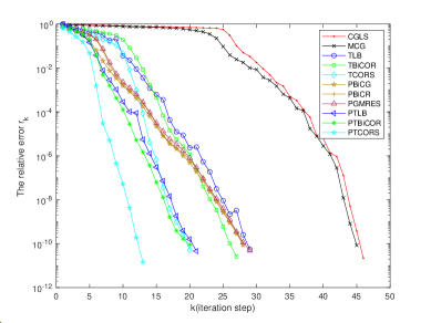
We set and let the initial tensor . The right-hand side of (1.1) is constructed by (1.1) with the exact solution of (1.3) derived by the MATLAB command in [7]. Algorithms 2-6 are used to solve (1.1) with the matrices in (6.1). These methods are compared with CGLS in [16] and MCG in [23], respectively.
Figure 1 shows the convergence of the relative error versus the number of iterations for all methods. From Figure 1, we can see that our preconditioned Algorithms 5-7 present better convergence than Algorithms 2-4 without preconditioning, PGMRES in [9], PBiCG and PBiCR in [30]. While Algorithms 2-4 can compare with PGMRES, PBiCG and PBiCR, and are better than CGLS [16] and MCG [23]. Algorithm 6 converges fastest among all algorithms. Algorithm 5 converges the second fastest among all algorithms.
Example 6.2.
Consider the convection-diffusion equation in [4, 29]
A standard finite difference discretization on equidistant nodes combined with the second order convergent scheme [20, 18] for the convection term leads to the linear system (1.1) with
(6.2)
where and the mesh-size .
Table 1: Comparison of the running time, total iteration number and the corresponding relative error for different method with different parameters when the criterion is satisfied for Example 6.2
Methods
time(s)
TIN
Methods
time(s)
TIN
CGLS
0.422117
131
9.7291e-11
PBiCG
0.407984
27
5.7115e-11
MCG
0.314574
130
9.1914e-11
PBiCR
0.333801
27
6.2653e-11
PGMRES
1.195048
26
8.4492e-11
TLB
0.439216
48
8.0006e-11
PTLB
0.413785
25
4.4981e-11
TBiCOR
0.379316
48
1.2006e-11
PTBiCOR
0.283238
24
4.5384e-11
TCORS
0.235870
32
7.9107e-11
PTCORS
0.202668
15
7.9490e-12
CGLS
0.420019
142
9.7422e-11
PBiCG
0.327606
39
7.7596e-11
MCG
0.349199
141
9.1934e-11
PBiCR
0.365583
39
7.7732e-11
PGMRES
2.643044
37
7.6420e-11
TLB
0.547317
57
2.2617e-11
PTLB
0.452652
24
6.9294e-11
TBiCOR
0.275463
51
6.4086e-11
PTBiCOR
0.240380
22
9.2513e-11
TCORS
0.199584
30
3.6561e-11
PTCORS
0.167069
13
1.5901e-11
CGLS
0.400485
137
7.8655e-11
PBiCG
0.345495
23
5.9009e-12
MCG
0.314983
136
7.9150e-11
PBiCR
0.420298
23
5.1618e-12
PGMRES
0.716276
20
2.9726e-11
TLB
0.490665
53
4.5843e-11
PTLB
0.412092
24
1.3665e-12
TBiCOR
0.431553
49
2.6997e-11
PTBiCOR
0.271265
22
6.3548e-11
TCORS
0.289261
29
4.6591e-11
PTCORS
0.182132
14
1.4634e-11
CGLS
0.619692
231
9.8161e-11
PBiCG
0.302540
24
9.6344e-11
MCG
0.479290
228
9.5604e-11
PBiCR
0.332252
25
1.8973e-11
PGMRES
0.969060
23
8.3597e-11
TLB
0.574761
60
6.1992e-11
PTLB
0.463983
25
6.7805e-11
TBiCOR
0.359788
59
6.2755e-11
PTBiCOR
0.294740
25
3.1182e-11
TCORS
0.259970
33
9.4662e-11
PTCORS
0.204611
15
1.2034e-11
CGLS
0.661334
234
8.5041e-11
PBiCG
0.321293
26
7.8704e-12
MCG
0.508388
231
9.1198e-11
PBiCR
0.435445
24
7.5118e-11
PGMRES
0.885821
22
7.6295e-11
TLB
0.500843
53
7.0480e-12
PTLB
0.360964
22
1.1481e-12
TBiCOR
0.275404
48
7.3762e-11
PTBiCOR
0.244606
20
5.4227e-11
TCORS
0.229283
28
1.0059e-12
PTCORS
0.146302
12
1.2266e-11
CGLS
0.658699
240
8.7261e-11
PBiCG
0.321684
39
9.3669e-11
MCG
0.517902
236
9.5783e-11
PBiCR
0.356874
38
9.4120e-11
PGMRES
2.472089
36
3.8573e-11
TLB
0.531822
55
6.9508e-11
PTLB
0.491639
29
8.5332e-12
TBiCOR
0.316190
54
5.6945e-11
PTBiCOR
0.268896
28
8.7378e-11
TCORS
0.203383
30
6.8170e-12
PTCORS
0.164989
16
2.5240e-12
We consider the case when and . The right-hand side is constructed by (1.1) with the exact solution of (1.3) produced by the MATLAB commend in [7].
Let the initial solution be a tensor with each element being zero. Algorithms 2-7 are used to solve (1.1) with given in (6.2). These methods are compared with CGLS [16], MCG [23], PGMRES in [9], PBiCG and PBiCR in [30].
Table 1 displays the running time, total iteration number (TIN) and relative error of different method with different parameters and .
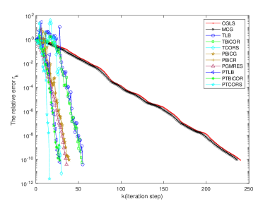
Figure 2 shows the convergence of the relative error for each method with the parameters , , and .
Table 1 shows that, when the stop criterion is satisfied, preconditioned Algorithms 5-6 require less CPU time and iterations than Algorithms 2-4, PGMRES, PBiCG and PBiCR. In most cases Algorithms 2-4 requires much less CPU time but more iterations than PGMRES, PBiCG and PBiCR, and are better than CGLS [16] and MCG [23] both in CPU time and the number of iterations. Algorithm 6 requires the minimal CPU time and iterations among all methods.
Figure 2 shows similar results to that in Figure 1.
Example 6.3.
We consider the Sylvester tensor equation (1.1) with the coefficient matrices , which comes from the discretization of the operator
(6.3)
on the unit square with homogeneous Dirichlet boundary conditions. We use the MATLAB command fdm_2d_matrix in the Lyapack package [25] to generate matrices :
(6.4)
where .
We construct by (1.1) with the exact solution of (1.3) produced by the MATLAB commend in [7].
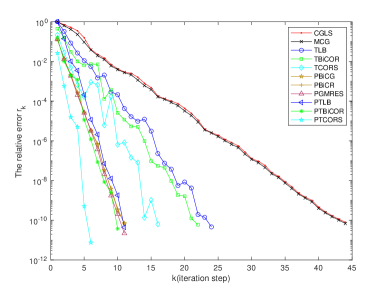
Figure 3: Plot of the relative error for Example 6.3.
The initial solution is selected as zero tensor. Algorithms 2-6 are used to solve (1.1) with given in (6.4). These methods are compared with CGLS [16], MCG [23], PGMRES in [9], PBiCG and PBiCR in [30].
Figure 3 shows that Algorithm 6 converges fastest among all methods and Algorithm 6 converges the second fastest among all methods, which are very similar to those in Figures 1 and 2.
7 Conclusion
This paper first presents a tensor Lanczos -Biorthogonalization (TLB) algorithm for solving the Sylvester tensor equation (1.1) based on the Lanczos -Biorthogonalization procedure. Then two improved methods based on the TLB algorithm are developed. The one is the biconjugate -orthogonal residual algorithm in tensor form (TBiCOR). The other is the conjugate -orthogonal residual squared algorithm in tensor form (TCORS). The preconditioner based on the nearest Kronecker product (NKP) are used to accelerate the TBiCOR and TCORS algorithms, thus we present preconditioned a preconditioned TBiCOR method and a preconditioned TCORS method. The convergence of these proposed algorithms are proved. Numerical examples show the advantage of the preconditioned TBiCOR and TCORS methods.
8 Acknowledgments
The authors would like to thank the referees for their helpful comments which form the present version of this paper. The preconditioned methods are added according to one comment. Research by G.H. was supported in part by Application Fundamentals Foundation of STD of Sichuan (2020YJ0366) and Key Laboratory of bridge nondestructive testing and engineering calculation Open fund projects (2020QZJ03), and research by F.Y. was partially supported by NNSF (11501392) and SUSE (2019RC09).
References
[1]F.A. Beik, F. Movahed, S. Ahmadi-Asl, On the Krylov subspace methods based on tensor format for positive definite Sylvester tensor equations, Numer. Linear Algebr. 23 (2016) 444-466.
[2] M. August, M.C. Banuls, T. Huckle, On the approximation of functionals of very large hermitian matrices represented as matrix product operators, Electron. T. Numer. Ana. 46 (2017) 215-232.
[3] Z.Z. Bai, G. Golub, M. Ng, Hermitian and skew-Hermitian splitting methods for non-Hermitian positive definite linear systems, SIAM J. Matrix Anal. Appl. 24 (2002) 603-626.
[4] J. Ballani, L. Grasedyck, A projection method to solve linear systems in tensor format, Numer. Linear Algebr. 20 (2013) 27-43.
[5] F.A. Beik, M. Najafi-Kalyani, L. Reiche, Iterative Tikhonov regularization of tensor equations based on the Arnoldi process and some of its generalizations, Appl. Numer. Math. 151 (2020) 425-447.
[6] A.H. Bentbib, S. El-Halouy, E.M. Sadek, Krylov subspace projection method for Sylvester tensor equation with low rank right-hand side, Numer. Alg. 84 (2020) 1411-1430.
[7] B.W. Bader, T.G. Kolda, Matlab tensor toolbox, Version 2.5, Available online at http://www.sandia.gov/tgkolda/TensorToolbox/, 2012.
[8] D. Calvetti, L. Reichel, Application of ADI iterative methods to the restoration of noisy images, SIAM J. Matrix Anal. Appl. 17 (1) (1996) 165-186.
[9] Z. Chen, L. Lu, A projection method and Kronecker product preconditioner for solving Sylvester tensor equations, SCI. China Ser. A. Math. 55 (2012) 1281-1292.
[10] Z. Chen, L. Lu, A Gradient Based Iterative Solutions for Sylvester Tensor Equations, Math. Probl. Eng. (2013) 1-7.
[11] B. Carpentieri, Y.F. Jing, T.Z. Huang, The BiCOR and CORS iterative algorithms for solving nonsymmetric linear systems, SIAM J. Sci. Comput. 33 (2011) 3020-3036.
[12] F. Ding, T. Chen, Gradient based iterative algorithms for solving a class of matrix equations, IEEE T. Automat. Contr. 50 (2005) 1216-1221.
[13] F. Ding, T. Chen, Iterative least-squares solutions of coupled Sylvester matrix equations, Syst. Contr. Lett. 54 (2005) 95-107.
[14] G. Golub, S. Nash, C. Van Loan, A Hessenberg-Schur method for the problem , IEEE T. Automat. Contr. 24 (1979) 909-913.
[15] M. Heyouni, F. Saberi-Movahed, A. Tajaddini, A tensor format for the generalized Hessenberg method for solving Sylvester tensor equations, J. Comput. Appl. Math. 377 (2020) 112878.
[16] B. Huang, C. Ma, An iterative algorithm to solve the generalized Sylvester tensor equations, Linear Multilinear A. 68 (2018) 1175-1200.
[18] D. Kressner, C. Tobler, Krylov subspace methods for linear systems with tensor product structure, SIAM J. Matrix Anal. Appl. 31 (2010) 1688-1714.
[19] D. Kressner, C. Tobler, Low-rank tensor Krylov subspace methods for parametrized linear systems, SIAM J. Matrix Anal. Appl. 32 (2011) 1288-1316.
[20] L. Grasedyck, Existence and computation of low Kronecker-rank approximations for large linear systems of tensor product structure, Computing 72 (2004) 247-265.
[21] B.W. Li, Y.S. Sun, D.W. Zhang, Chebyshev collocation spectral methods for coupled radiation and conduction in a concentric spherical participating medium, J. Heat Trans. 131 (2009) 1-9.
[22] N. Li, C. Navasca, C. Glemn, Iterative methods for symmetric outer product tensor decomposition, Electron. T. Numer. Ana. 44 (2015) 124-139.
[23] C. Lv, C. Ma, A modified CG algorithm for solving generalized coupled Sylvester tensor equations, Appl. Math. Comput. 365 (2020) 124699.
[24] M. Najafi-Kalyani, F.A. Beik, K. Jbilou, On global iterative schemes based on Hessenberg process for (ill-posed) Sylvester tensor equations, J. Comput. Appl. Math. 373 (2020) 112216.
[25] T. Penzl, Lyapack, A MATLAB toolbox for large Lyapunov and Riccati equations, model reduction problems,and linear-quadratic optimal control problems, Available online at https://www.tu-chemnitz.de/sfb393/lyapack/, 2000.
[26] Y. Saad, Iterative methods for sparse linear systems, Society for Industrial and Applied Mathematics, 2nd edition, 2003.
[27] X.H. Shi, Y.M. Wei, S.Y. Ling, Backward error and perturbation bounds for high order Sylvester tensor equation, Linear Multilinear A. 61 (2013) 1436-1446.
[28] C.F. Van Loan, N. Pitsianis, Approximation with Kronecker products, In Proc.: Linear Algebra for Large Scale and Real-Time Applications, Kluwer Publications 232 (1993) 293-314.
[29] H. Xiang, L. Grigori, Kronecker product approximation preconditioners for convection-diffusion model problems, Numer. Linear Algebr. 17 (2010) 691-712.