Exploring Features in the Binary Black Hole Population

Abstract

Vamana is a mixture model framework that infers the astrophysical distribution of chirp mass, mass ratio, and spin component aligned with the orbital angular momentum for the binary black holes (BBH) population. We extend the mixing components in this framework to also model the redshift evolution of merger rate and report all the major one and two-dimensional features in the BBH population using the 69 gravitational wave (GW) signals detected with a false alarm rate $<1\mathrm{yr}^{-1}$ in the third Gravitational Wave Transient Catalog (GWTC)-3. Endorsing our previous report and corroborating recent report from LIGO Scientific, Virgo, and KAGRA Collaborations, we observe the chirp mass distribution has multiple peaks and a lack of mergers with chirp masses $10\textrm{--}12M_{\odot}$. In addition, we observe aligned spins show mass dependence with heavier binaries exhibiting larger spins, mass ratio shows a dependence on the chirp mass but not on the aligned spin, and the redshift evolution of the merger rate for the peaks in the mass distribution is disparate. These features possibly reflect the astrophysics associated with the BBH formation channels. However, additional observations are needed to improve our limited confidence in them.

1 Introduction

LIGO Scientific, Virgo and KAGRA Collaborations (LVK) recently released GWTC-2.1, a deep extended catalog of observations made during the first half of the third observation run (O3a) (Abbott et al., 2021d). This was followed by the release of GWTC-3, a catalog inclusive of observations made during the second half of the third observation run (O3b) (Abbott et al., 2021e). Observation of GW signals have also been reported in previous catalogs GWTC-1 and GWTC-2 (Abbott et al., 2019a, 2021a). Advanced LIGO and advanced Virgo (Aasi et al., 2015; Acernese et al., 2015) have now detected a total of 69 BBH observations at a false alarm rate of less than once per year.

These observations have begun to probe the BBH population and have presented many unexpected surprises. The observation of massive binary, GW150914 (Abbott et al., 2016), was in contrast to the early on expectation of observing lighter binaries (Bailyn et al., 1998; Fryer & Kalogera, 2001; Özel et al., 2010; Farr et al., 2011). Observations of multiple low-spin binaries as measured from the GW (Farr et al., 2017, 2018; Tiwari et al., 2018) contrasts the high spin black hole companion in various x-ray binary measurements (Gou et al., 2011; Miller et al., 2009; McClintock et al., 2006, 2011; Miller & Miller, 2015; Fishbach & Kalogera, 2021). And, an interesting and somewhat surprising feature in the BBH population is an emerging structure in the mass distribution. The observations tend to cluster around multiple peaks. In addition, there is a gap in the chirp mass distribution lacking mergers in the range 10–12$M_{\odot}$ (Tiwari & Fairhurst, 2021; Abbott et al., 2021f).

Observations have further expanded on these features, indicating that lighter binaries contribute significantly to the total merger rate (Abbott et al., 2019a, 2021a, 2021d, 2021e), black holes in heavier binaries tend to have larger spin magnitude (Tiwari & Fairhurst, 2021; Galaudage et al., 2021; Hoy et al., 2021), and as reported in this article the early results indicate the merger rate evolves with redshift, but, at different rate for the peaks in the mass distribution.

Periodic increase in the number of observations has motivated multiple reports on the BBH population (Talbot & Thrane, 2018; Wysocki et al., 2019; Abbott et al., 2019b; Roulet & Zaldarriaga, 2019; Abbott et al., 2021b; Roulet et al., 2021; Abbott et al., 2021f). In this article, we report on the features in the BBH population inferred by the mixture model framework Vamana (Tiwari, 2021) using the GW observations detected in GWTC-3. This article is laid out as follows: We briefly discuss the analysis in Section 2, the features in the predicted population in Section 3, some features in the context of hierarchical merger scenario in Section 4 and astrophysical implication in Section 5.

2 Data Selection and Analysis

Gravitational wave observations made in the last three observation runs have been reported over multiple catalogs (Abbott et al., 2019a, 2021a, 2021d, 2021e). We analyse the BBH mergers reported with a false alarm rate of at most once per year. Independent searches have reported additional GW observations (Nitz et al., 2019, 2020; Zackay et al., 2019; Venumadhav et al., 2020) but we leave these observations out due to lack of a framework that can self consistently combine results from independent search analysis. As we restrict our analysis to BBH, we exclude binaries that have at least one component consistent with a neutron star. They are, GW170817, GW190425, GW200105, GW190917, GW200105, GW200115 (Abbott et al., 2017, 2020a, 2021c, 2021e). Finally, we also exclude GW190814 (Abbott et al., 2020b), which has secondary mass substantially different from the remaining BBH observations ($\sim 2.6M_{\odot}$) and its exclusion is not expected to impact the inference on the bulk BBH population (Essick et al., 2021). The total number of selected observations is 69.

We use the mixture model framework Vamana to predict the population (Tiwari, 2021). Vamana uses a mixture of components, each composed of a Gaussian, another Gaussian, and a power-law to model the chirp mass, both the aligned spin components, and mass ratio respectively. Similar to multiple previous works, the redshift evolution of merger rate is modeled using a Single power-law with exponent $\kappa$ quantifying the merger rate evolution for the full population (Fishbach et al., 2018; Abbott et al., 2019b; Callister et al., 2020; Roulet et al., 2020; Abbott et al., 2021b, f),

$$\mathcal{R}(z)=\mathcal{R}\,(1+z)^{\kappa},$$ (1)

where $\mathcal{R}$ is the population averaged merger rate at $z=0$. Some features of the population inferred using Vamana for the GWTC-3 observations have already been reported (Abbott et al., 2021f). In this article we report features not presented earlier. In addition, we report inference made using the Mixed model created by assigning mixture component independent $\kappa$ values. This extension facilitated separable modeling of the redshift evolution for the merger rate in different regions of parameter space and resulted in the identification of an additional feature at a moderate credibility: the redshift evolution of the merger rate shallows for the fourth peak in the chirp mass distribution.

We use a Jefferey’s prior for the Single model, defined as (Grigaityte & Atwal, 2019),

$$p(\kappa)\propto\frac{1}{|1+k|},\quad\mathrm{for}\;|1+\kappa|\in[0.1,10],$$ (2)

and assign a uniform prior for $\kappa$ between -1.1 and -0.9 such that distribution is piecewise continuous. For the Mixed analysis we facilitate separable modeling by letting components choose uniformly between $\kappa_{i}-3$ and $\kappa_{i}+3$, for a $\kappa_{i}$ sampled from the prior distribution in Equation 2. The choice of range is arbitrarily chosen to allow the components to have few orders of magnitude variation in merger rate at a redshift of one. In practice, a bigger interval allows for more variation, but for large values of $\kappa$, inference on population hyper-parameters are inaccurate due to the errors incurred in the importance sampling employed in the Bayesian analysis (Tiwari, 2021). Although we use a sufficiently open model, as $\kappa$ values outside this range are also supported by the data, the median and credible intervals presented in this article is subjected to our chosen prior. Our choice on the remaining hyper-parameter priors and their ranges for the Mixed model remain unchanged compared to the Single model (please refer to appendix B.1.d in Abbott et al. (2021f) for the complete description). Our inference is robust for a wide range of component numbers in the mixture. We use eleven components in the presented analysis as this choice maximises the marginal likelihood.

The observed binary population is biased compared to the true astrophysical distribution due to the selective sensitivity of the gravitational wave network towards BBH masses and spins. This bias is corrected by estimating the sensitivity of the searches towards simulated signals added to the data set (Tiwari, 2018). The large-scale simulation runs performed to estimate this sensitivity has been obtained using the waveform model SEOBNRv4PHM (Bohé et al., 2017; Ossokine et al., 2020). To reduce any systematic difference between simulations for sensitivity estimation and Parameter Estimation (PE) samples of the GW signals, we preferentially choose the PE samples obtained using the same waveform model, wherever available. However, using combined PE samples from SEOBNRv4PHM and IMRPhenomXPHM (Pratten et al., 2021), as used in Abbott et al. (2021f), has only a small effect on the results. The binary parameters are estimated in the detector frame, to change to the source frame quantities we use the Planck15 cosmology (Ade et al., 2016). All the PE samples and simulation campaign’s data is publicly available (The LIGO Scientific Collaboration & the Virgo Collaboration, 2019; LIGO Scientific, Virgo and KAGRA Collaborations, 2021).

Although Mixed model introduces ten additional hyper-parameters, the marginal likelihood for both Single and Mixed models is approximately the same. Unless otherwise noted, all the numerical results reported in this article are for the Mixed model with the median as the central value along with the 90% credible interval.

3 The Binary Black Hole Population

In this section we discuss the various features in the binary black hole population.

3.1 Mass Distribution

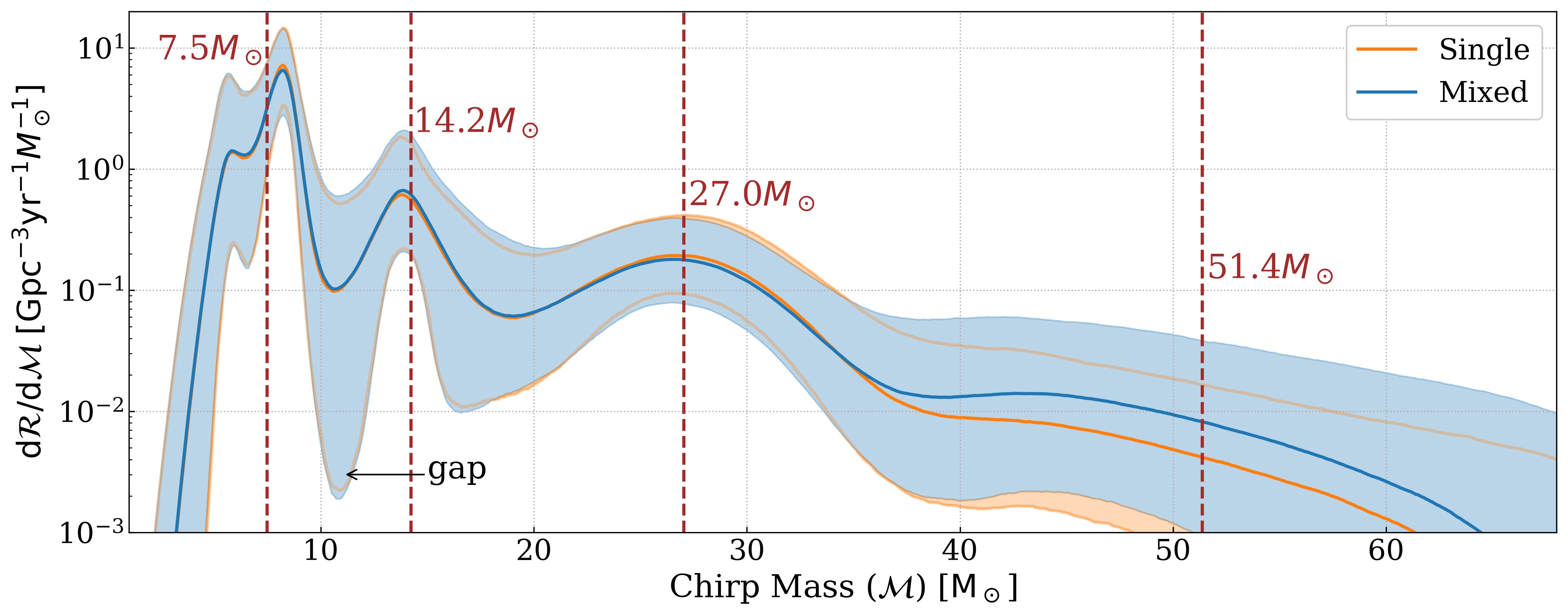
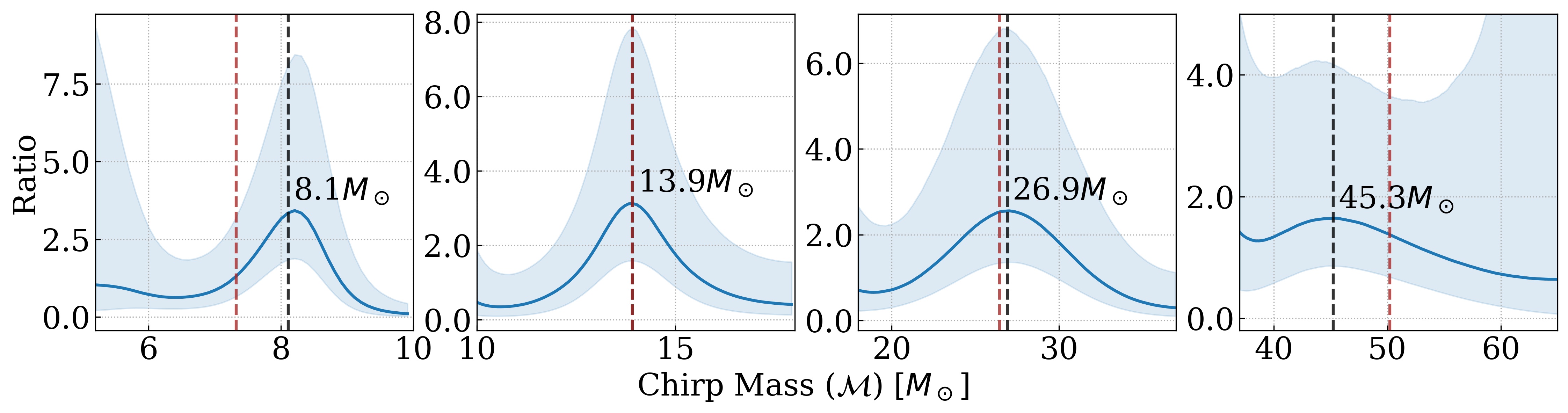
Figure 1: Top) The predicted one-dimensional chirp mass distribution at $z=0$. The solid line shows the posterior median and the shaded regions (light solid line when hidden) show the 90% credible interval. The chirp mass distribution shows presence of a number of peaks. The lack of mergers in the chirp mass range $10-12M_{\odot}$ is labeled as ’gap’. Starting at an arbitrarily chosen chirp mass value, the dashed brown lines are placed at a factor of 1.9. Bottom) The brown lines match well with the location of the peaks. The location of the peaks is the local maxima in the blue curve and indicated by the black dashed line. The blue curve is the median of ratio between the posterior and prior chirp mass density, each truncated and normalised for the shown interval. The shaded region is the 50% credible region.

Peak	Chirp Mass Range	Local Maxima	Credibility
1	5.2–10	8.1	93
2	10–18	13.9	88
3	18–37	26.9	86
4	37–67	45.3	70

Table 1: We define four chirp mass intervals that enclose the peaks. We make random draws from the posterior and prior chirp mass density. For each interval, we truncate and normalise these densities, and calculate the ratio between them. We define a peak at the chirp mass value where this ratio is greater than one at the highest credibility. Here, we define credibility as the percentage of draws with a ratio greater than one at a given mass value. In this table, we summarise the choice on intervals, location of the peaks and our confidence in them. All masses are in $M_{\odot}$.

In a previous article, we reported an emerging structure in the mass distribution (Tiwari & Fairhurst, 2021). Independent analyses have reported similar features since then (Edelman et al., 2021; Sadiq et al., 2021; Li et al., 2021; Veske et al., 2021; Rinaldi & Del Pozzo, 2021). Our previous population predictions were based on 39 observations reported in GWTC-2. The addition of newly reported or previously ignored observations (we used stricter selection criteria in the previous analysis), 30 in number, has kept the structure intact (Abbott et al., 2021f). The observations cluster around four peaks and there is a lack of mergers in the chirp mass range 10–12 $M_{\odot}$. The upper panel in Fig. 1 shows the predicted chirp mass distribution and the lower panel shows the location of the peaks. Each peak occurs at approximately double the mass of the previous peak. We have a substantial confidence in the presence of the first peak, the second and the third peak, and a marginal confidence in the presence of the fourth peak. We quantify the location of the peaks and our confidence in them in Table 1.

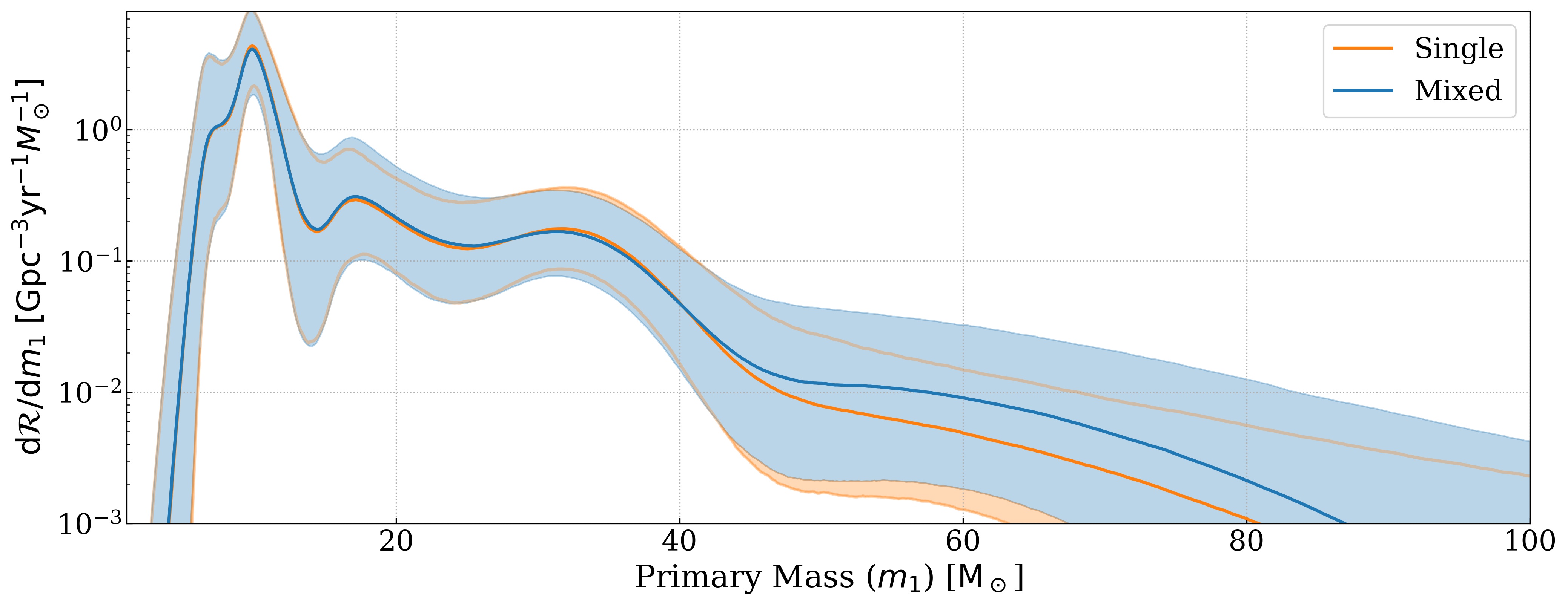
Figure 2: The predicted primary mass distribution for the two redshift models at redshift $z=0$. The solid line is the median distribution and the shaded region (light solid line when hidden) shows the 90% credible interval. The primary mass distribution shows a similar structure, and although the locations of the peaks are different compared to their locations on the chirp mass distribution, their relative location bears similar factors. This is understandable as mass ratio distribution shows only a weak dependence on the chirp mass (please see section 3.4).

Fig. 2 shows the predicted primary mass distribution. A similar structure can be observed. Compared to Fig. 1, the peaks are located at different mass values, but the locations bear a similar factor. The features are less pronounced compared to the chirp mass distribution. Possibly, because the mass ratio is not measured precisely. It is also possible that the astrophysical primary mass distribution does not exhibit peak as prominently as the chirp mass distribution, however, that will require a unique combination of primary mass and mass ratio distributions. Although we do not show the component or the secondary mass distributions they exhibit similar structure. We note that the mass of black holes in the three reported neutron star–black hole binaries (GW190917, GW200105, and GW200115) are consistent with the first peak in the primary mass distribution (Abbott et al., 2021c, e). We also note that most of the observations, reported in multiple independent searches, but not included in the presented analysis, also follow this clustering (Venumadhav et al., 2020; Zackay et al., 2019; Nitz et al., 2019, 2020, 2021).

3.2 Spin and Mass Ratio Distribution

Fig. 3 shows the one-dimensional mass ratio and aligned spin distributions obtained by marginalising over other parameters. Similar to results post GWTC-2, the mass ratio is well modeled by a decaying power law. Ninety five percent of the binaries have a mass-ratio of greater than half. For the second half of the third observation run there has been an increase in the fraction of binaries that exhibit higher spin magnitudes, thus the aligned distribution has slightly broadened since our last report (Tiwari & Fairhurst, 2021).

The choice of the power-law function in modeling the mass ratio will inadvertently impact the measurement of the spins as the two parameters are significantly correlated (Baird et al., 2013; Tiwari et al., 2018). Due to this correlation, the mass ratio is measured less accurately, thus also impacting the measurement of the component masses. Among the multiple phenomenological distributions we have tested to model the mass ratio, the marginal likelihood is maximised when using a power law.

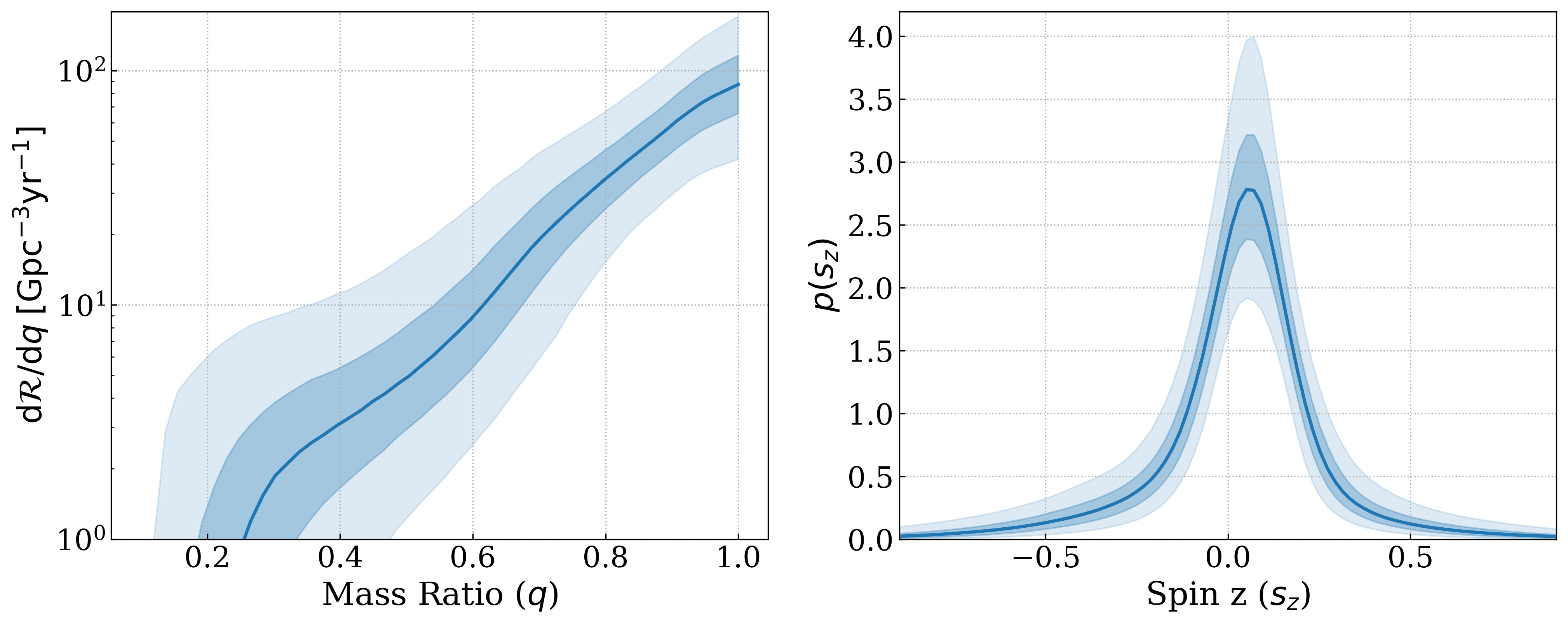
Figure 3: The predicted one-dimensional mass ratio and aligned spin distributions. Left) The solid line is the distribution median and the shaded regions show the 50% and the 90% credible interval. The mass ratio distribution is peaked towards equal masses, with 95% of support above 0.47. Right) The predicted aligned spin distribution shows support for small aligned spins, with the distribution, peaked near zero, and 90% of the distribution is contained within the range [-0.41, +0.39]. The one-dimensional distribution is dominated by low mass binaries; all of them have been measured with low spin magnitude. The spins show a correlation with the chirp mass which we discuss in section 3.4.

3.3 Redshift Evolution of Merger Rate

We estimate the population averaged BBH merger rate to be ${18.4}^{+{12.6}}_{-{8.3}}\,\mathrm{Gpc}^{-3}\,\mathrm{yr}^{-1}$ at $z=0$. This is consistent with the merger rate reported in Abbott et al. (2021f). The merger rate corresponding to chirp mass intervals listed in Table 1 are reported in Table 2. The first chirp mass interval contributes around 70% of the mergers. Fig. 4 shows the posterior on the merger rate and its evolution with the redshift. For both the models, the merger rate is increasing with redshift at credibility greater than 95%.

Interval	5.2–10	10–18	18–37	37–67
$\mathcal{R}$	$12.8^{+9.5}_{-6.0}$	$2.4^{+3.1}_{-1.5}$	$2.0^{+2.4}_{-1.2}$	$0.1^{+0.2}_{-0.8}$
$\kappa$	$2.7^{+3.2}_{-3.0}$	$1.7^{+3.5}_{-3.2}$	$2.4^{+2.1}_{-2.0}$	$0.6^{+3.1}_{-2.9}$

Table 2: Merger rate and it’s evolution corresponding to each chirp mass interval in Table 2. All units are in $\mathrm{Gpc}^{-3}\mathrm{yr}^{-1}$ and all masses are in $M_{\odot}$.

The Single model assigns the same redshift evolution to the whole population. For this model, we measure $\kappa=2.3^{+1.8}_{-2.1}$. The Mixed model assigns a separate $\kappa$ for a mixing component and facilitates independent modeling of merger rate evolution for different regions of the population. We recover the mass dependence by marginalising $\kappa$ over the chirp mass intervals listed in Table 2. We report the aggregate $\kappa$’s associated with each peak in Table 1. In addition, similar information is portrayed in Fig. 5 where we plot the fractional increase in merger rate from $z=0$ to $z=0.5$ as dependent on the chirp mass. The credible intervals are large but there may be initial hints that the merger rate evolution associated with the peaks are disparate. The lack of observations, especially at higher redshift, for the second and the fourth interval results in shallower evolution of merger rate. In particular, the merger rate evolution for the fourth chirp mass interval is shallower compared to the rest of the BBH population at a credibility of 90%. As mentioned earlier, our inferences are subjected to our choice of the prior on $\kappa$. However, our confidence in this feature increases/decreases on increasing/decreasing the flexibility of the analysis in modeling the rate evolution (please refer to Section 2 for a discussion on this). The third peak, which is confined in the chirp mass interval 18 to 37$M_{\odot}$, contributes to more than half of the observed GW signals. We do not observe a notable mass evolution in this range as shown in Fig. 5. This figure also shows the predicted observations (selection applied to population prediction), which are consistent for both the models for most of the chirp mass range. However, the Mixed model predicts lower redshift values at higher chirp masses.

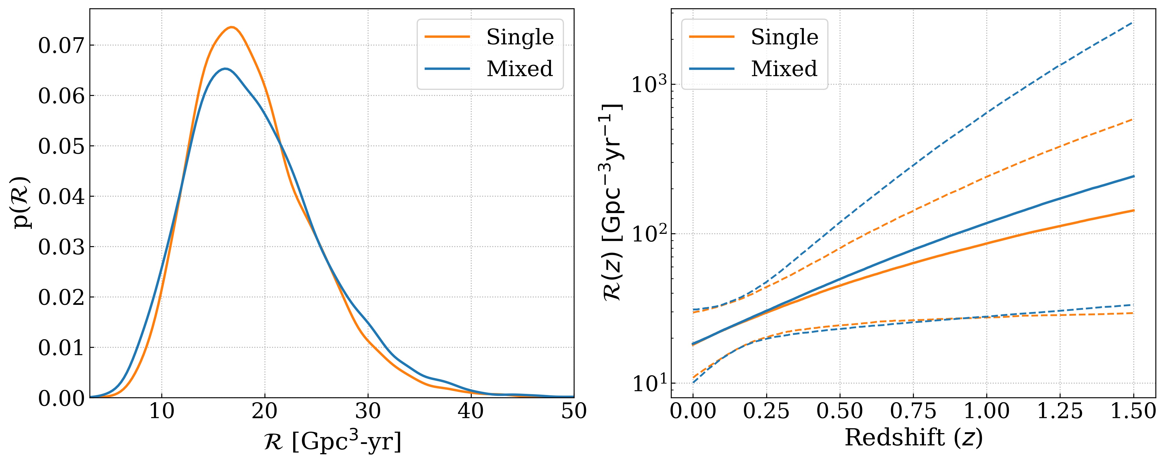
Figure 4: Left) The merger rate of binary black-holes in the local universe for the two redshift models. The BBH merger rate for the Mixed model is ${18.4}^{+{12.6}}_{-{8.3}}\,\mathrm{Gpc}^{-3}\,\mathrm{yr}^{-1}$. Right) The redshift evolution of the merger rate. Solid curves are the median distribution and dashed curves enclose the 90% credible intervals. The Mixed model shows a steeper increase in the merger rate.

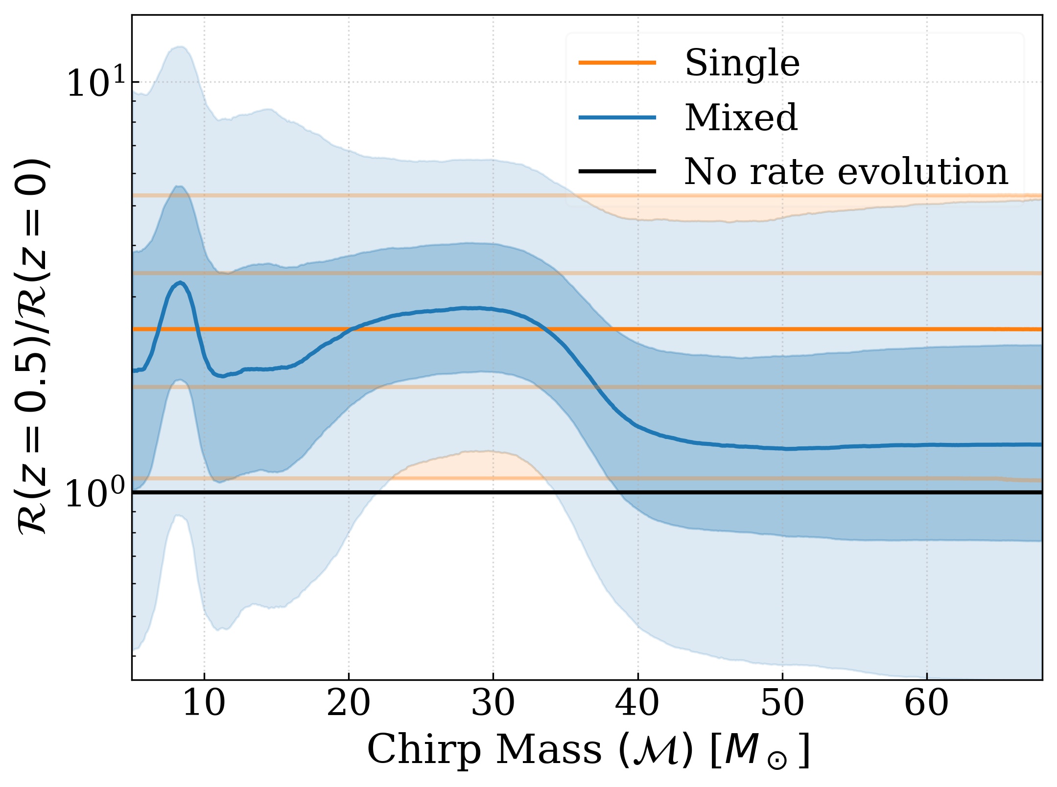
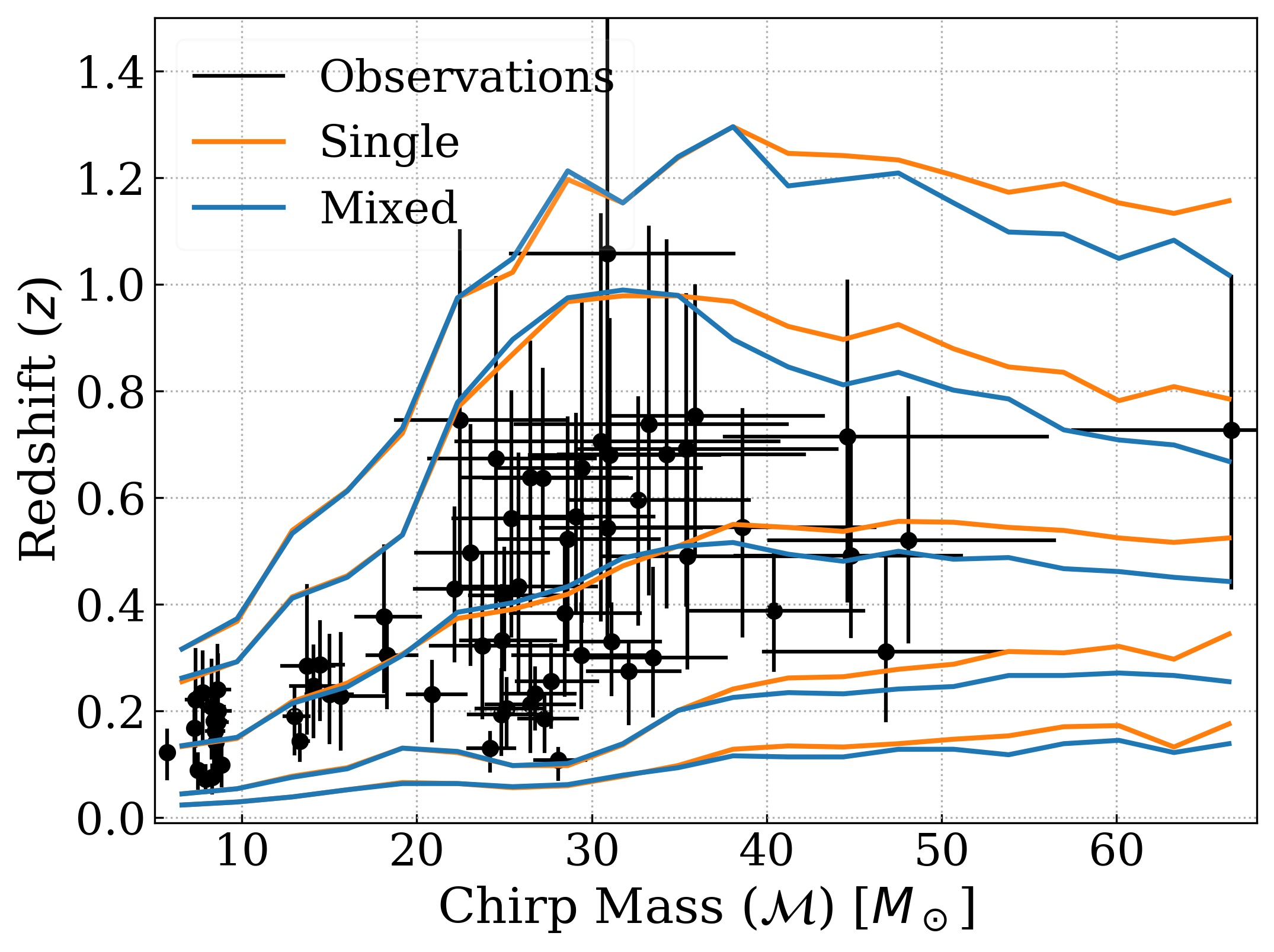
Figure 5: Left) The dependence of the redshift evolution of the merger rate on the chirp mass. The vertical axes shows the ratio of merger rate between $z=0$ and $z=0.5$. The light/dark band (or light solid lines if hidden) is the 90%/50% credible interval and the dark solid curve is the median distribution. The blue bands, that correspond to the Mixed model, show shallowing of merger rate at the second and the fourth peak. Right) Comparing selection weighted prediction with the observations. We apply selection effects to the predicted population and obtain multiple realisations of expected observations. We record the minimum, maximum, and median redshift values for each realisation. The top two curves are the $95^{\mathrm{th}}$ and $75^{\mathrm{th}}$ percentile of the maximum values, the bottom two curves are the $5^{\mathrm{th}}$ and $25^{\mathrm{th}}$ percentile of the minimum values and the middle curve is the median of the median values. The black crosses are measurements from the GW observations. Both the models predict equivalent distribution for most of the chirp mass range with Mixture model making predictions at relatively smaller redshift values for heavier masses.

3.4 Correlated Features

The mixture model framework allows us to model correlations present among the population’s signal parameters (chirp mass, mass ratio aligned spin, or redshift distributions). Once we have obtained the posterior on model hyper-parameters, $\Lambda$, we can predict the population distribution, $p(\theta|\Lambda)$, for the signal parameter, $\theta$.

Fig. 6 shows the variation of the mass ratio and aligned spin as a function of the chirp mass. The mass ratio shows a weak correlation with the chirp mass. Most of the binaries are of comparable masses throughout the chirp mass range. The distribution shows increased asymmetry at the second peak. This is mainly due to GW190412 and multiple observations that have a mass ratio of around one-half. The binaries corresponding to the third peak show least asymmetry. A phenomenological treatment of this feature is reported in Li et al. (2022). The spins are consistent with small magnitude for most of the chirp mass range but show an increase for chirp masses $30M_{\odot}$ or more. The 90% credible interval for aligned spins averaged over chirp masses 30$M_{\odot}$ or less is [-0.41, +0.38], that increases to [-0.55, +0.62] for chirp masses 30$M_{\odot}$ or more. Vamana models aligned spin for both the black holes to be independent but identically distributed. We do not observe a correlation between aligned spin and mass-ratio as shown in Fig. 7 . The aligned spin distribution is devoid of a trend. We stress that the correlation observed between parameters is seldom independent. A change in an inferred correlation caused due to waveform systematic or change in priors can also lead to a changed inference between other parameters. This is especially relevant for heavier masses where chirp mass, mass ratio, and spin degeneracy are strong.

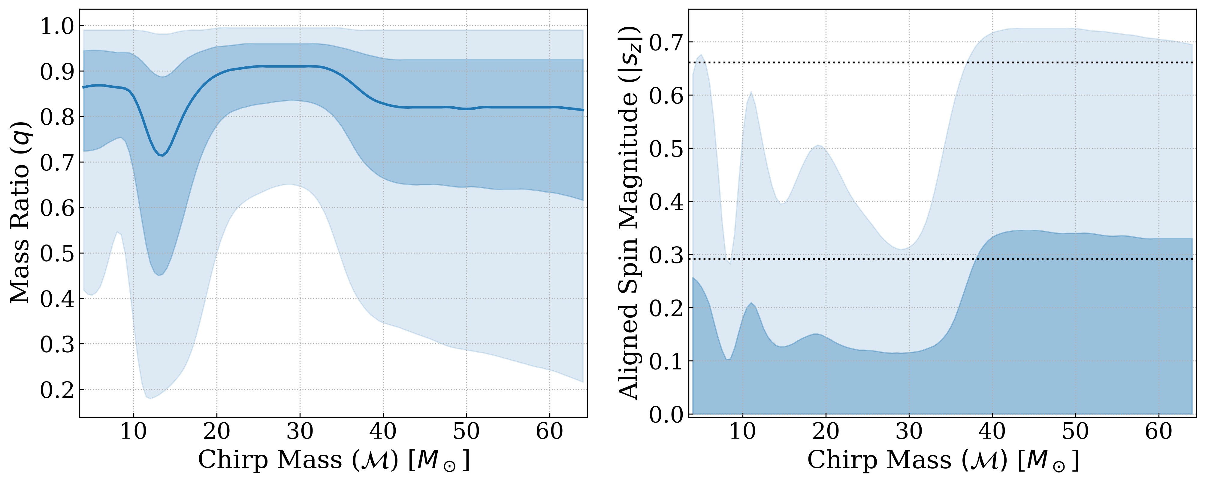
Figure 6: The variation of mass ratio and aligned spin magnitude with the chirp mass. Left) The solid curve is the median and the light/dark bands are the 90%/50% credible intervals. Around 95% of the mergers are consistent with mass ratios of 0.5 or more. The mass ratio show dependence on the chirp mass. Binaries consistent with the second/third peak are most/least asymmetric. Right) The light/dark bands are the magnitude of the aligned spin at 90%/50% credibility. The aligned spin magnitude is consistent with small values for most of the chirp mass range, however, it increases for chirp mass values of 30 $M_{\odot}$ or more. The dotted lines are aligned spin’s 50% and 90% credible bounds of the prior distribution.

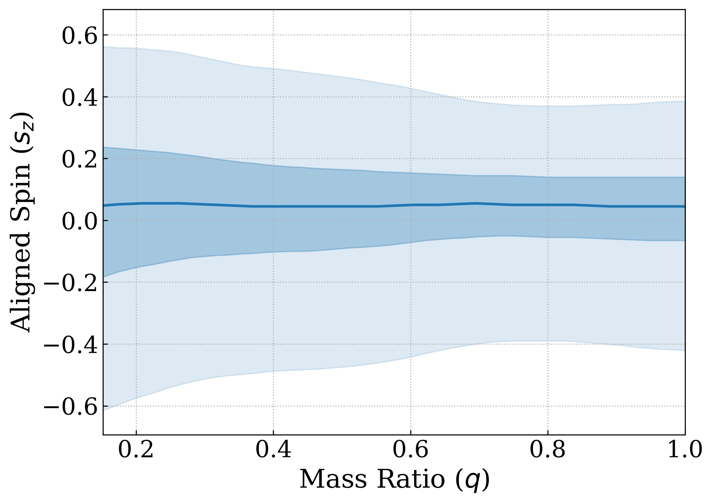
Figure 7: The variation of the aligned spin with the mass ratio. Solid curve is the median distribution, and the light/dark bands are the 90%/50% credible intervals. The aligned spin is consistent with very small values and does not seem to show a correlation throughout the mass ratio range.

4 The Hierarchical Merger Scenario

Similar to the suggestion in our previous article (Tiwari & Fairhurst, 2021), we discuss the observed features in the BBH population in the context of hierarchical mergers.

Peaks and lack of mergers: In simplest terms, the lack of observations in the chirp mass range 10–12$M_{\odot}$ and four well-placed peaks can be explained with the first peak populated from binaries that have black holes produced from stellar evolutionary process and following peaks due to hierarchical merger scenario (Miller & Hamilton, 2002; Antonini & Rasio, 2016; Rodriguez et al., 2019; Doctor et al., 2021; Gerosa & Fishbach, 2021; Mapelli et al., 2021). Fig. 1 suggests, starting at the first peak black holes merge to successively produce heavier black holes. The location of these peaks bears a factor of around 1.9. Such a factor would naturally arise from a hierarchical merger scenario as the remnant produced from the merger of black holes is slightly less massive than the total mass of the binary due to around 5% loss of mass in gravitational waves.

Spins: Arguably, the most robust prediction for a hierarchical merger scenario is highly spinning remnants (Campanelli et al., 2007; González et al., 2007; Buonanno et al., 2008; Berti & Volonteri, 2008; Baibhav et al., 2021; Mahapatra et al., 2021). Even if we assume that black holes in the first peak/generation to have low spins, the black holes in the second or higher generation should display high spins. And although spins do increase with the masses as seen in Fig. 6 they are consistent with small magnitudes for most of the chirp mass range.

Cross- generation mergers: Hierarchical merger scenarios often predict cross generation mergers. Black holes in the first peak/generation(G) can also merge with the heavier ones which are remnant of a previous merger. In fact, many combinations exist resulting in mergers with mass ratios of one-half, one-fourth etc., and giving rise to intermediate peaks located between the primary peaks. Among these, 1G+2G mergers are expected to be most dominant (Rodriguez et al., 2019; Arca Sedda et al., 2020), but, we are not observing these mergers as their observation will fill the gap in the 10-12$M_{\odot}$ chirp mass range. However there are some hints of cross-generation mergers. The chirp masses for 1G+3G mergers will overlap with the second peak. GW190412 is an example that has it’s chirp and component masses consistent with a 1G+3G merger. In addition, it was observed with moderate spins. Observations GW190408 and GW191215 with chirp mass of around 19 $M_{\odot}$ are consistent with a 2G+3G merger but are neither observed with a mass-ratio of one-half nor with high spins. However, an emerging peak at this chirp mass value will be of interest.

5 Astrophysical Implications

The mass spectrum has retained the structure after the addition of new observations. Thus, all of the implications we made earlier still remain valid (Tiwari & Fairhurst, 2021).

The mass distribution of field binaries is expected to follow a power law like distribution with the maximum mass of the binaries sensitive to the metallicity and the initial mass function of the progenitor stars. The metallicity of stars impacts the mass loss due to stellar winds (Heger et al., 2003; Belczynski et al., 2010; Postnov & Yungelson, 2014). The mean metallicity decreases with redshift (Madau & Dickinson, 2014). At lower metallicities, the black hole mass distribution is expected to extend to higher masses. Pair-instability supernovae can impose an upper limit on the maximum mass of the binary as well as introduce a build-up at high masses (Fowler & Hoyle, 1964; Rakavy et al., 1967; Bond et al., 1984; Heger & Woosley, 2002). Thus, population synthesis models that simulate complex physics of stellar evolution expect the maximum black-hole to many tens of solar mass. However, the results presented here provide evidence for a lack of black hole binaries in the chirp mass range 10–12 $M_{\odot}$. The median differential rate decays by a factor of around 60 in this range. In addition, there is a presence of peaks in the mass distribution which possibly evolve disproportionately with the redshift. We expect these features to be of interest to the population synthesis models.

BBH formation and merger can also be facilitated within the star clusters  (Sigurdsson & Hernquist, 1993; Portegies Zwart & McMillan, 2000; Rodriguez et al., 2015; Antonini & Rasio, 2016; Gerosa & Berti, 2019). This could include their formation in active galactic nuclei (Stone et al., 2017; Gröbner et al., 2020; Yang et al., 2019; Tagawa et al., 2021; Gayathri et al., 2021) or formation of binaries due to scattering in galactic cusps (O’Leary et al., 2009). The mass spectrum can potentially inform about the many-body dynamics in the star clusters. Specifically, the relative amplitude and the width of the peaks could provide information about the host environment.

The population has several other features. The spin distribution is consistent with low magnitudes for most of the mass range but heavier binaries also tend to exhibit larger spins. The mass ratio distribution shows a weak dependence on the chirp mass but not on spins. These multifarious population properties are of interest for analysis attempting to explain observation as a mix of multiple formation channels. Many proposed scenarios predict the formation of binaries in a wide mass range (Abadie et al., 2010; Mandel & Broekgaarden, 2021) and it is possible to estimate contributions from various formation channels that can give rise to the observed distribution (Hütsi et al., 2021; Zevin et al., 2021; Wong et al., 2021; Ng et al., 2021). However, more observations are needed to ascertain if a unique combination can give rise to the observed population properties.

The hierarchical merger scenario offers a simple explanation for the location of four well-placed peaks. Our suggestion as hierarchical mergers to be the dominant source for the peaks require addressing a few issues including the issues outlined in Sec. 4. This scenario opens up various other avenues for investigation. The relative location of peaks will quantify the percentage loss of mass in GW and will therefore provide an opportunity to test general relativistic predictions of energy emission due to the merger. Although the absolute location of the peaks depends on the assumed cosmology, their relative location should remain unchanged within the framework of standard cosmology. This creates an opportunity to test non-standard cosmological models. Predicted features in the mass spectrum do not provide any non-gravitational information and thus cannot be used to estimate Hubble’s constant. But, if a feature can be identified in the source mass-spectrum (Messenger & Read, 2012; Farr et al., 2019) it is conceivable to conduct a combined test of general relativity and cosmology.

6 Conclusions

In this article we reported on the BBH population predicted using the observations made during LVK first, second, and third observation runs. Endorsing our previous report and corroborating LVK’s recent report, we find the mass distribution has four emerging peaks and a lack of mergers in the chirp mass range 10–12$M_{\odot}$. The population exhibits a small spin magnitude for most of the mass range that increases monotonically for the heavier masses. The mass ratio distribution shows dependence on the chirp mass but not on the aligned spin. We observe possible hints that the redshift evolution of the merger rate is disparate for the peaks in the mass distribution. We expect these features to have large implications on our understanding of the BBH formation channels, however, as our results are limited by small statistics we await LVK’s fourth observation run which promises to significantly increase the number of observations.

Data Availability

The code used in performing the presented analysis and the corresponding result files are available at https://github.com/vaibhavtewari/vamana.

References

- Aasi et al. (2015) Aasi, J., Abbott, B. P., Abbott, R., Abbott, T., et al. 2015, Classical and Quantum Gravity, 32, 074001, doi: 10.1088/0264-9381/32/7/074001
- Abadie et al. (2010) Abadie, J., Abbott, B. P., Abbott, R., et al. 2010, Classical and Quantum Gravity, 27, 173001, doi: 10.1088/0264-9381/27/17/173001
- Abbott et al. (2016) Abbott, B. P., Abbott, R., Abbott, T. D., et al. 2016, Phys. Rev. Lett., 116, 061102, doi: 10.1103/PhysRevLett.116.061102
- Abbott et al. (2017) —. 2017, Phys. Rev. Lett., 119, 161101, doi: 10.1103/PhysRevLett.119.161101
- Abbott et al. (2019a) —. 2019a, Physical Review X, 9, 031040, doi: 10.1103/PhysRevX.9.031040
- Abbott et al. (2019b) —. 2019b, ApJ, 882, L24, doi: 10.3847/2041-8213/ab3800
- Abbott et al. (2020a) —. 2020a, ApJ, 892, L3, doi: 10.3847/2041-8213/ab75f5
- Abbott et al. (2020b) Abbott, R., Abbott, T. D., Abraham, S., et al. 2020b, ApJ, 896, L44, doi: 10.3847/2041-8213/ab960f
- Abbott et al. (2021a) —. 2021a, Physical Review X, 11, 021053, doi: 10.1103/PhysRevX.11.021053
- Abbott et al. (2021b) —. 2021b, ApJ, 913, L7, doi: 10.3847/2041-8213/abe949
- Abbott et al. (2021c) —. 2021c, ApJ, 915, L5, doi: 10.3847/2041-8213/ac082e
- Abbott et al. (2021d) Abbott, R., Abbott, T. D., Acernese, F., et al. 2021d, arXiv e-prints, arXiv:2108.01045. https://arxiv.org/abs/2108.01045
- Abbott et al. (2021e) —. 2021e, arXiv e-prints, arXiv:2111.03606. https://arxiv.org/abs/2111.03606
- Abbott et al. (2021f) —. 2021f, arXiv e-prints, arXiv:2111.03634. https://arxiv.org/abs/2111.03634
- Acernese et al. (2015) Acernese, F., Agathos, M., Agatsuma, K., et al. 2015, Classical and Quantum Gravity, 32, 024001, doi: 10.1088/0264-9381/32/2/024001
- Ade et al. (2016) Ade, P. A. R., Aghanim, N., Arnaud, M., et al. 2016, A&A, 594, A13, doi: 10.1051/0004-6361/201525830
- Antonini & Rasio (2016) Antonini, F., & Rasio, F. A. 2016, ApJ, 831, 187, doi: 10.3847/0004-637X/831/2/187
- Arca Sedda et al. (2020) Arca Sedda, M., Mapelli, M., Spera, M., Benacquista, M., & Giacobbo, N. 2020, ApJ, 894, 133, doi: 10.3847/1538-4357/ab88b2
- Baibhav et al. (2021) Baibhav, V., Berti, E., Gerosa, D., Mould, M., & Wong, K. W. K. 2021, Phys. Rev. D, 104, 084002, doi: 10.1103/PhysRevD.104.084002
- Bailyn et al. (1998) Bailyn, C. D., Jain, R. K., Coppi, P., & Orosz, J. A. 1998, ApJ, 499, 367, doi: 10.1086/305614
- Baird et al. (2013) Baird, E., Fairhurst, S., Hannam, M., & Murphy, P. 2013, Phys. Rev. D, 87, 024035, doi: 10.1103/PhysRevD.87.024035
- Belczynski et al. (2010) Belczynski, K., Bulik, T., Fryer, C. L., et al. 2010, ApJ, 714, 1217, doi: 10.1088/0004-637X/714/2/1217
- Berti & Volonteri (2008) Berti, E., & Volonteri, M. 2008, ApJ, 684, 822, doi: 10.1086/590379
- Bohé et al. (2017) Bohé, A., Shao, L., Taracchini, A., et al. 2017, Phys. Rev. D, 95, 044028, doi: 10.1103/PhysRevD.95.044028
- Bond et al. (1984) Bond, J. R., Arnett, W. D., & Carr, B. J. 1984, ApJ, 280, 825, doi: 10.1086/162057
- Buonanno et al. (2008) Buonanno, A., Kidder, L. E., & Lehner, L. 2008, Phys. Rev. D, 77, 026004, doi: 10.1103/PhysRevD.77.026004
- Callister et al. (2020) Callister, T., Fishbach, M., Holz, D. E., & Farr, W. M. 2020, ApJ, 896, L32, doi: 10.3847/2041-8213/ab9743
- Callister et al. (2021) Callister, T. A., Haster, C.-J., Ng, K. K. Y., Vitale, S., & Farr, W. M. 2021, ApJ, 922, L5, doi: 10.3847/2041-8213/ac2ccc
- Campanelli et al. (2007) Campanelli, M., Lousto, C., Zlochower, Y., & Merritt, D. 2007, ApJ, 659, L5, doi: 10.1086/516712
- Doctor et al. (2021) Doctor, Z., Farr, B., & Holz, D. E. 2021, ApJ, 914, L18, doi: 10.3847/2041-8213/ac0334
- Edelman et al. (2021) Edelman, B., Doctor, Z., Godfrey, J., & Farr, B. 2021, Available as arxiv:2109.06137, arXiv:2109.06137. https://arxiv.org/abs/2109.06137
- Essick et al. (2021) Essick, R., Farah, A., Galaudage, S., et al. 2021, arXiv e-prints, arXiv:2109.00418. https://arxiv.org/abs/2109.00418
- Farr et al. (2018) Farr, B., Holz, D. E., & Farr, W. M. 2018, ApJ, 854, L9, doi: 10.3847/2041-8213/aaaa64
- Farr et al. (2019) Farr, W. M., Fishbach, M., Ye, J., & Holz, D. E. 2019, ApJ, 883, L42, doi: 10.3847/2041-8213/ab4284
- Farr et al. (2011) Farr, W. M., Sravan, N., Cantrell, A., et al. 2011, ApJ, 741, 103, doi: 10.1088/0004-637X/741/2/103
- Farr et al. (2017) Farr, W. M., Stevenson, S., Miller, M. C., et al. 2017, Nature, 548, 426, doi: 10.1038/nature23453
- Fishbach et al. (2018) Fishbach, M., Holz, D. E., & Farr, W. M. 2018, ApJ, 863, L41, doi: 10.3847/2041-8213/aad800
- Fishbach & Kalogera (2021) Fishbach, M., & Kalogera, V. 2021, arXiv e-prints, arXiv:2111.02935. https://arxiv.org/abs/2111.02935
- Fowler & Hoyle (1964) Fowler, W. A., & Hoyle, F. 1964, ApJS, 9, 201, doi: 10.1086/190103
- Fryer & Kalogera (2001) Fryer, C. L., & Kalogera, V. 2001, ApJ, 554, 548, doi: 10.1086/321359
- Galaudage et al. (2021) Galaudage, S., Talbot, C., Nagar, T., et al. 2021, arXiv e-prints, arXiv:2109.02424. https://arxiv.org/abs/2109.02424
- Gayathri et al. (2021) Gayathri, V., Yang, Y., Tagawa, H., Haiman, Z., & Bartos, I. 2021, ApJ, 920, L42, doi: 10.3847/2041-8213/ac2cc1
- Gerosa & Berti (2019) Gerosa, D., & Berti, E. 2019, Phys. Rev. D, 100, 041301, doi: 10.1103/PhysRevD.100.041301
- Gerosa & Fishbach (2021) Gerosa, D., & Fishbach, M. 2021, Nature Astronomy, 5, 749, doi: 10.1038/s41550-021-01398-w
- González et al. (2007) González, J. A., Sperhake, U., Brügmann, B., Hannam, M., & Husa, S. 2007, Phys. Rev. Lett., 98, 091101, doi: 10.1103/PhysRevLett.98.091101
- Gou et al. (2011) Gou, L., McClintock, J. E., Reid, M. J., et al. 2011, ApJ, 742, 85, doi: 10.1088/0004-637X/742/2/85
- Grigaityte & Atwal (2019) Grigaityte, K., & Atwal, G. 2019, bioRxiv, doi: 10.1101/664243
- Gröbner et al. (2020) Gröbner, M., Ishibashi, W., Tiwari, S., Haney, M., & Jetzer, P. 2020, A&A, 638, A119, doi: 10.1051/0004-6361/202037681
- Heger et al. (2003) Heger, A., Fryer, C. L., Woosley, S. E., Langer, N., & Hartmann, D. H. 2003, ApJ, 591, 288, doi: 10.1086/375341
- Heger & Woosley (2002) Heger, A., & Woosley, S. E. 2002, ApJ, 567, 532, doi: 10.1086/338487
- Hoy et al. (2021) Hoy, C., Fairhurst, S., Hannam, M., & Tiwari, V. 2021, arXiv e-prints. https://arxiv.org/abs/2110.13542
- Hütsi et al. (2021) Hütsi, G., Raidal, M., Vaskonen, V., & Veermäe, H. 2021, J. Cosmology Astropart. Phys, 2021, 068, doi: 10.1088/1475-7516/2021/03/068
- Li et al. (2021) Li, Y.-J., Wang, Y.-Z., Han, M.-Z., et al. 2021, ApJ, 917, 33, doi: 10.3847/1538-4357/ac0971
- Li et al. (2022) Li, Y.-J., Wang, Y.-Z., Tang, S.-P., et al. 2022, arXiv e-prints, arXiv:2201.01905. https://arxiv.org/abs/2201.01905