Projection-based Classification of Surfaces for 3D Human Mesh Sequence Retrieval

Abstract

We analyze human poses and motion by introducing three sequences of easily calculated surface descriptors that are invariant under reparametrizations and Euclidean transformations. These descriptors are obtained by associating to each finitely-triangulated surface two functions on the unit sphere: for each unit vector $u$ we compute the weighted area of the projection of the surface onto the plane orthogonal to $u$ and the length of its projection onto the line spanned by $u$. The $L_{2}$ norms and inner products of the projections of these functions onto the space of spherical harmonics of order $k$ provide us with three sequences of Euclidean and reparametrization invariants of the surface. The use of these invariants reduces the comparison of 3D+time surface representations to the comparison of polygonal curves in ${\mathbb{R}}^{n}$. The experimental results on the FAUST and CVSSP3D artificial datasets are promising. Moreover, a slight modification of our method yields good results on the noisy CVSSP3D real dataset.

1 Introduction

Comparing 3D surfaces is a challenging problem lying at the heart of many primary research areas in computer graphics, computer vision applications and medical applications. The main difficulty when comparing two triangulated surfaces is that their triangulations do not necessarily have the same number of triangles and, even if they did, there is no natural way to discern what the corresponding triangles would be in each triangulation. The goal of analyzing shapes of surfaces modulo re-triangulations or reparametrizations—their continuous analogues—leads to enormous computational challenges. These are further complicated by the need in many applications to identify surfaces that differ only by Euclidean transformations and similarities.

A particularly elegant mathematical approach to the problem of comparing surfaces is to consider the quotient of the space of embeddings of a fixed surface $S$ into ${\mathbb{R}}^{3}$ by the actions of the orientation-preserving diffeomorphisms of $S$ and the group of Euclidean transformations, and provide this quotient with the structure of an infinite-dimensional orbifold. We can then define and use Riemannian metrics on this orbifold to measure the distance between two given shapes as well as to interpolate between them by computing the (generally unique) geodesic that joins them  ([1],  [2]). Another exciting approach is that of square root normal fields or SRNF in which different embeddings and immersions of the surface $S$ modulo translations are described by points in a Hilbert space, and both rotations in ${\mathbb{R}}^{3}$ as well as reparametrizations of the surface translate into orthogonal transformations in the Hilbert space  ([3]). Both approaches are very general and, in theory at least, permit the perfect or nearly perfect comparison of large classes of shapes. Nevertheless, there are many situations were we would need or prefer a quicker and rougher tool to distinguish, classify, or retrieve shapes from a restricted population of surfaces. An example of such a situation is the subject of this work: the classification and retrieval of human poses and actions. Furthermore, the articulation of the human body enables it to adopt a great variety of poses with very small changes to the intrinsic geometry of the surface that models it. In flexing an arm or a leg we mostly see small intrinsic changes due to the bulging and stretching of muscles, but the net result in terms of the extrinsic geometry of the body can be substantial. Small changes in the intrinsic geometry may even lead to apparent changes in the genus of the human figure through topological noise when, for instance, hands are clasped or feet and legs are crossed. This points to the unsuitability of approaches that we will call intrinsic, and which are focused on the metric relations (lengths of curves, angles, and areas) on the surface itself independently of the embedding into the ambient space.

In the analysis and retrieval of human actions we must work with sequences of a hundred human poses, and each pose is represented by a triangulated surface containing thousands or tens of thousands of vertices. This computational complexity is nevertheless offset by the fact that human poses are modeled by a rather restricted population of surfaces. Examination of the databases led us to formulate the hypothesis that a human pose is nearly characterized by its convex hull. The intuition is that if you enclose someone in a tight, perfectly elastic sheet, the different poses of this person will still be distinguishable, or mostly so (see Figure 1). In considering human body motion, where there is a sequence of poses, the probability of recognition of the action from the associated sequence of convex hulls should be even greater, or so the intuition goes.

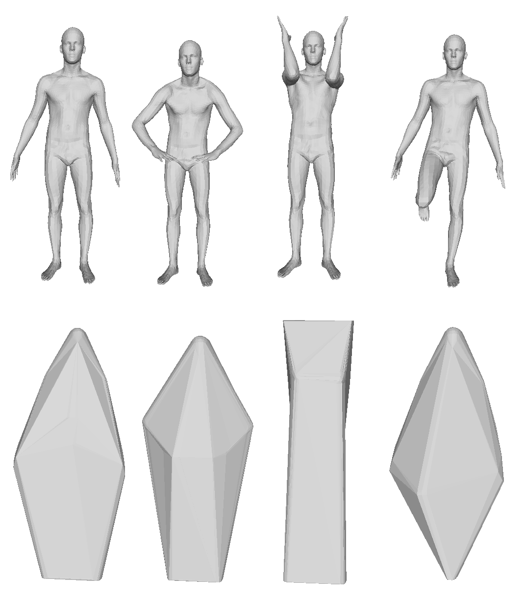
Fig. 1: Four human poses from the FAUST dataset along with their corresponding convex hulls.

This convexity hypothesis led to the idea of considering two of the most basic notions in convex geometry, the convex hull and the surface area measure or extended Gaussian image (EGI), and molding them into three sequences of numerical surface descriptors that are invariant under Euclidean transformations. We do this by first encoding the information of the convex hull in the breadth function, which measures the length of the projection of the surface onto each line passing through the origin, and encoding the information of the EGI in the weighted area function, which for each direction measures the weighted area of the projection of the surface onto the plane perpendicular to it (see Section 3 for details). These functions only depend on symmetrizations of the convex hull and EGI (Proposition 3.2 and Theorem 3.5), but are supplementary (i.e., two non-convex surfaces with the same symmetrized convex hull are not likely to have the same symmetrized EGI) and lend themselves nicely to Fourier analysis. Our three sequences of numerical shape descriptors are obtained as the $L_{2}$ norms and inner products of the projections of these functions onto the space of spherical harmonics of order $k$. In geophysics terminology, these are the power spectra and the cross power spectrum of our two functions ( [4],  [5], and see [6] for the introduction of this idea in the context of shape matching).

The main concern of this paper is the problem of analyzing human motion and our numerical descriptors conveniently allow us to reformulate it as a problem of comparing polygonal curves in ${\mathbb{R}}^{n}$. In this familiar setting we make use of dynamic time warping (DTW) to compare the curves obtained from the CVSSP3D real and synthetic datasets [7].

In this paper we did not pay close attention to the effect that noisy data could have on our methods and to the interesting problem of how to make them more robust, but we did test them against the relatively noisy CVSSP3D real dataset (see Table 5) and remarked that a slight modification to our breadth function to make it more robust yielded good results.

Overall, the contributions of this paper can be summarized as follows.

• We present a novel set of descriptors invariant under parametrization, Euclidean transformations, and scaling.

• We formulate the problem of comparing sequences of 3D human surfaces as a problem of comparing curves in ${\mathbb{R}}^{n}$. Dynamic Time Warping (DTW) is proposed for temporal alignment of these curves.

• The method shows promising results for 3D pose and 3D motion retrieval tasks in several datasets. The results are promising and validate our hypothesis that the analysis of human action can be in good measure reduced to the analysis of sequences of convex hulls of human poses.The experimental results show that our method can be be implemented in a computationally efficient way due to its simple formulation.

Plan of the paper. In Section  2, we review some recent works that have tackled the same or related problems. In Section 3 we present the mathematical foundation of our work and the construction of the three sequences of Euclidean and shape invariants. This section culminates with the definition of the feature vectors and polygonal curves with which we analyze surfaces and surface motions. The experimental setup is described in Section 4. There we present the evaluation criteria, the datasets, and the results of static pose analysis on the FAUST dataset before moving on to tackle the dynamic analysis of motion in the CVSSP3D synthetic and real dataset. Finally, we present the mean computation times for the construction of the different polygonal curves associated to the human motions in the various datasets. Lastly, conclusions and discussion are reported in Section 5.

2 Related Work

2.1 Static geometric descriptors

The challenge in comparing two shapes is to find the best measure of similarity over the space of all transformations. The need for efficient retrieval makes it impractical to explicitly query against all transformations, and two different approaches have been proposed. In the first approach shapes are placed into a canonical coordinate frame (normalizing for translation, scale and rotation) and two shapes are assumed to be aligned when each is in its own frame. Thus, the best measure of similarity can be found without explicitly trying all possible transformations. The second approach describes 3D models through a geometric invariant descriptor so that all transformations of a model result in the same descriptor. Some descriptors are shown in Table 1, which describes how these methods address translation, scale and rotation. Other descriptors are intrinsic: they are defined by local metric properties on the surface itself and, therefore, have natural translation and rotation invariance. They are better suited for shape retrieval than for pose retrieval since the intrinsic geometric differences of the surfaces modeling the human body in different poses are not necessarily significant. Examples of these descriptors are HKS, WKS and ShapeDNA, presented in Table 1. We refer the reader to [8] for an extensive review and comparison of such descriptors.

Representation	Tr	Sc	Rot
Shape Distributions [9] [6]	I	N	I
Extended Gaussian Images [10] [6]	I	N	N
Shape Histograms [11] [6]	N	N	N
Heat Kernel Signatures  [12] [13]	I	N	I
Wave Kernel Signature  [14]	I	I	I
ShapeDNA [15]	I	N	I
GDVAE [16] (Deep learning)	I	N	I
Neural3DMM [17] (Deep learning)	N	N	N

Table 1: A summary of a number of shape descriptors, showing whether they are (I)nvariant with respect to translation, scaling and rotation, or whether they require (N)ormalization.

2.2 Deep Learning

Deep learning for 3D human poses attracts more and more attention. These new approaches require the reformulation of several deep learning operations, such as regular convolution and pooling/unpooling to the non-regular mesh. Bronstein et al. [18] give a comprehensive overview of the generalization of CNNs on non-Euclidean manifolds. More recently several deep learning approaches propose to learn a latent representation with disentangled shape and pose components. Zhou et al. [17] propose an auto-encoder model that disentangles shape and pose for 3D meshes in an unsupervised manner. However, the proposed neural network requires mesh correspondence, while our approach does not. Aumentado-Armstrong et al. [16] propose a two-level unsupervised Variational Autoencoder (GDVAE), with a disentangled latent space. They utilize point cloud data to learn a latent representation of 3D human shape and thus require training to encode the shape and the pose. They utilize the fact that isometric deformations preserve the spectrum of the Laplace-Beltrami Operator (LBO). The LBO is a popular way of capturing intrinsic shape. However, the spectrum is very sensitive to noise as shown in our experiments.

2.3 3D shape sequence retrieval

Huang et al. [19] extended shape distribution, Spin Image, and spherical harmonics to 3D human motion retrieval. These shape descriptors are not necessarily related to the geometry of human body. Slama et al. [20] propose a 3D human motion analysis framework for shape similarity and retrieval. The shape descriptor, called Extremal Human Curve (EHC), is a set of 10 curves which connect the extremal points of the 3D human surface. The authors of [20] propose a geometric approach for comparing the shapes of human surfaces via EHC. They exploit the fact that curves can be parameterized canonically and thus can be compared naturally. However, the need of the detection of extremal points makes this approach sensitive to the noise and to the low quality of the meshes. In addition, the comparison between pairs of curves increase the computational cost. Another interesting approach is presented by Luo et al. [21], where they compute a spatio-temporal graph of 3D Human motion. However, this approach also suffers from being time consuming, and needs the same parameterization along a dataset to perform well. In  [22] six static shape descriptors are extracted from each mesh of the human sequence and DTW is used as similarity measure, before proposing to add other information like centroid position and speed. However, some descriptors used in this approach requires a pose normalization for each mesh per frame using two variations of PCA.

3 Projection-based classification of surfaces

3.1 The breadth representation

As we mentioned in the introduction, the guiding idea of this paper is that human poses seem to be determined to a great extent by their convex hulls (see Figure 1). In order to quantify and test this hypothesis, we consider the support and breadth functions of the triangulated surfaces that model the human form.

Definition 3.1

The support function of a set $S\subset{\mathbb{R}}^{n}$ evaluated at the unit vector $u\in S^{n-1}$ is the quantity

$$h(S;u):=\sup_{x\in S}\,u\cdot x.$$

The breadth of the set $S\subset{\mathbb{R}}^{n}$ in the direction given by the unit vector $u\in S^{n-1}$ is the quantity

$$b(S;u):=h(S;u)+h(S,-u)=\sup_{x\in S}\,u\cdot x-\inf_{x\in S}\,u\cdot x\ .$$

Geometrically speaking, the breadth of a path-connected set in a direction $u$ is simply the length of the orthogonal projection of the set onto a line parallel to $u$. As the following classic result shows, the support function is a way to encode the convex hull.

Proposition 3.2

Two sets $S_{1},S_{2}\subset{\mathbb{R}}^{n}$ have the same support function if and only if their convex hulls are equal. Their breadth functions are the same if and only the convex hulls of the sets $S_{1}-S_{1}$ and $S_{2}-S_{2}$ are equal.

Proof. The convex hull of a set is the intersection of all half-spaces that contain it. From the definition of the support function, for each unit vector $u$, the half-space

$$H(S;u):=\{x\in{\mathbb{R}}^{n}:u\cdot x\leq h(S;u)\}$$

contains $S$ and is minimal in the sense that it is the unique half-space that contains $S$ and is contained in $H(S;u)$. From this perspective, the support function is just a way to encode the set of minimal half-spaces, and thus the set of all half-spaces, that contain $S$. It follows that the support function of a set characterizes its convex hull.

From the linearity of the functions $x\mapsto u\cdot x$ and the definition of support function, we have that if $A$ and $B$ are two subsets of ${\mathbb{R}}^{n}$, and $\lambda_{1}$ and $\lambda_{2}$ are two positive numbers, then

$$h(\lambda_{1}A+\lambda_{2}B;u)=\lambda_{1}h(A;u)+\lambda_{2}h(B;u)\textrm{ and }h(-A,u)=h(A;-u).$$

From this we conclude that the breadth function of a set $S$ is also the support function of $S-S$:

$$b(S;u)=h(S;u)+h(S;-u)=h(S-S;u).$$

Since the convex hull of a set is characterized by its support function, we conclude that the convex hulls of the sets $S_{1}-S_{1}$ are the same if and only if the breadth functions of $S_{1}$ and $S_{2}$ are equal.

Unlike the breadth function, the support function is not invariant under translations. This can be fixed by moving the center of mass to the origin. Generally speaking, there is less loss of information when working with the support function than with the breadth function, and this should come up in comparing surfaces that have a central symmetry to those that do not. However, for comparing human figures this did not seem to be the case and we made the choice to work with the breadth function to keep within a geometric tomography framework of studying human shapes through their projections onto lines and planes.

Using that triangles are convex and that the functions $x\mapsto u\cdot x$ $(u\in S^{2})$ are linear, the breadth of a triangulated surface $M\subset{\mathbb{R}}^{3}$ can be easily computed from just the knowledge of its vertex points $x_{1},\ldots,x_{N}$:

$$b(M;u):=\max_{1\leq i\leq N}\,u\cdot x_{i}-\min_{1\leq i\leq N}\,u\cdot x_{i}\ .$$

3.2 Area representation

Another classical descriptor of convex bodies and surfaces is the surface area measure or, as is better known in computer vision, the extended Gaussian image (EGI). This is the push-forward of the two-dimensional Hausdorff measure of the surface onto the unit sphere under the Gauss map. For a triangulated surface, we can give a more pedestrian equivalent formulation:

Definition 3.3

Given an oriented triangulated surface $M\subset{\mathbb{R}}^{3}$ formed by a union of triangles $T_{1}\ldots,T_{m}$, its extended Gaussian image is the measure on the unit sphere

$$\mu_{M}:=\sum_{i=1}^{m}\textrm{area}(T_{i})\,\delta_{n_{i}},$$

where $n_{i}$ is the unit vector perpendicular to $T_{i}$ in the sense defined by the orientation of the surface and $\delta_{n_{i}}$ is the delta measure concentrated at $n_{i}$.

There are a number of ways to extract feature vectors from the EGI of a surface. We can, for instance, manufacture them from the moments or the Fourier transform of this measure, but in this work we chose a more intuitive descriptor: the weighted area function.

Definition 3.4

Given an oriented triangulated surface $M\subset{\mathbb{R}}^{3}$ formed by a union of triangles $T_{1}\ldots,T_{m}$, its weighted area function is the function on the unit sphere defined by

$$\mathcal{A}(M;u):=\sum_{i=1}^{m}|u\cdot n_{i}|\,\textrm{area}(T_{i}),$$

where $n_{i}$ is a unit vector perpendicular to the triangle $T_{i}$.

The quantity $\mathcal{A}(M;u)$ is the weighted area of the projection of $M$ onto the plane orthogonal to $u$. By weighted area we mean that if $k$ different portions of a surface project onto the same piece of plane, the area of this piece is multiplied by $k$.

Besides being invariant under reparametrizations and translations, the weighted area function is easy to grasp geometrically and very quickly computed. It’s relation to the EGI of the surface follows directly from the definitions:

$$\mathcal{A}(M;u)=\int_{S^{2}}|u\cdot n|\,d\mu_{M}.$$

This expression immediately implies that surfaces with the same EGI are indistinguishable by the weighted areas of their projections. Moreover, because the functions $x\mapsto|u\cdot x|$ $(u\in S^{2})$ are even, we only see the even part of the measure $\mu_{M}$,

$$\mu^{e}_{M}=\frac{1}{2}\sum_{i=1}^{m}\textrm{area}(T_{i})\,(\delta_{n_{i}}+\delta_{-n_{i}}).$$

It follows that if the even parts of the surface area measures of two oriented surfaces are the same, then their weighted area functions are identical. This is all: by a theorem of Choquet ([23, p. 53]), finite linear combinations of the functions $x\mapsto|u\cdot x|$ $(u\in S^{2})$ are dense in the space of even continuous functions on the sphere, and hence if the integrals of all functions of this form with respect to two even measures are the same, the measures must be the same. We summarize:

Theorem 3.5

Two oriented triangulated surfaces $M_{1},M_{2}\subset{\mathbb{R}}^{3}$ are indistinguishable by the weighted areas of their projections if and only if the even parts of their extended Gaussian images are the same.

In order to use the weighted area function as a descriptor it is important to understand that if we decompose a surface into a finite or countable number of pieces each of which has a computable area, translating these pieces or flipping them around the origin, and then recomposing them again will give a new surface whose projection onto any plane has the same weighted area as that of the original surface. For instance, if we wish to make use of this technique to classify poses of a human figure it is useful to keep in mind the following rule of thumb: if we approximate and decompose the human body as the union of a number of boxes and then these boxes are moved by pure translation and re-glued into a different pose, the method will not effectively distinguish the old and the new poses. An important example is a person standing up with the arms by his/her side and the same person standing up with the arms straight up over his/her head (see Fig. 2).

Fig. 2: Different poses with the same weighted area function, but with different breadth functions.

Because of this “cut-translate-and-paste” invariance, the weighted area may not seem to be as good a descriptor as the breadth, and indeed, that is what our results confirm (see Table 2), but it is supplementary information and can be quite discerning in its own right. The weighted area allows us to distinguish some non-convex surfaces that have the same convex hull or breadth function, and although it is possible for two different non-convex surfaces to have the same convex hull and EGI—and, a fortiori, the same breadth and weighted area functions—without being translates (see Figure 3 for a simple two-dimensional example of these phenomena), that does not seem to happen to any significant degree in the restricted population of human poses. Nevertheless, the real advantage of considering simultaneously the breadth and weighted area functions will become clearer when we tackle the problem of extracting Euclidean invariants from these functions.

Fig. 3: The first two forms have the same convex hull and different weighted area functions, while the last two forms have the same convex hull and EGI.

3.3 Euclidean and shape invariants

In many applications it is not enough to be able to distinguish or classify surfaces up to reparametrizations and translations. Often we need to do so up to Euclidean transformations or up to similarities. In this section we describe a simple method to extract sequences of Euclidean and shape invariants from the area and breadth function of a surface.

Notice that if $M\subset{\mathbb{R}}^{3}$ is a surface and $R$ is a $3\times 3$ orthogonal matrix, then

$$\mathcal{A}(RM;u)=\mathcal{A}(M;R^{-1}u)\ \textrm{and}\ b(RM;u)=b(M,R^{-1}u)$$

for every unit vector $u$. In other words, the assignments $M\mapsto\mathcal{A}(M;\cdot)$ and $M\mapsto b(M;\cdot)$ are $O(3)$-equivariant maps between the space of surfaces and the space $L_{2}(S^{2})$ of square-integrable functions on the sphere provided with the usual left $O(3)$-action $(R,f)\mapsto f\circ R^{-1}$. The classic theory of spherical harmonics (see Lecture 11 of [24] for a particularly simple description) tells us that this space decomposes into the direct sum

$$L_{2}(S^{2})={\mathbb{R}}\oplus V_{1}\oplus V_{2}\oplus\cdots,$$

where $V_{k}$ is the $(2k+1)$-dimensional space of spherical harmonics of order $k$ (i.e., the restriction to the sphere of homogeneous harmonic polynomials of order $k$ in ${\mathbb{R}}^{3}$). These subspaces are invariant under the action of the orthogonal group and are mutually orthogonal. It follows that if $f$ is a square integrable function on the sphere, we can decompose $f=f_{0}+f_{1}+f_{2}+...$ with $f_{k}\in V_{k}$, and that the $L_{2}$ norm of each component $f_{k}$, defined by

$$\|f_{k}\|_{2}^{2}:=\frac{1}{4\pi}\int_{S^{2}}f_{k}(u)^{2}\,d\Omega,$$

is invariant under the orthogonal group. Notice that if the function $f$ is an even function, all the odd terms, $f_{2k+1}$, $k\geq 0$, are zero. This method to extract rotation invariants from spherical functions is classical (see, for instance, [25]) and is widely used in geophysics ([4, 5]), but in the context of computer science it seems to have been introduced in [6], where the term energy representation of $f$ is used for the sequence $k\mapsto\|f_{k}\|_{2}$.

Applying this idea to the area and breadth functions of a surface $M$ we obtain two sequences of invariants

$$\alpha_{k}(M):=\ \|\mathcal{A}_{2k}(M;\cdot)\|_{2}\ \ \textrm{and}\ \ \beta_{k}(M):=\|b_{2k}(M;\cdot)\|_{2}.$$

To this we add the sequence $\gamma_{k}(M)$ consisting of the inner products of $\mathcal{A}_{2k}(M;\cdot)$ and $b_{2k}(M;\cdot)$:

$$\langle\mathcal{A}_{2k}(M;\cdot),b_{2k}(M;\cdot)\rangle_{2}=\frac{1}{4\pi}\int_{S^{2}}\mathcal{A}_{2k}(M;u)b_{2k}(M;u)\,d\Omega,$$

which is also a Euclidean invariant of the surface $M$.

Using the equality

$$\|f+g\|_{2}^{2}=\|f\|_{2}^{2}+2\langle f,g\rangle_{2}+\|g\|_{2}^{2},$$

we have that

$$\gamma_{k}(M)=\frac{1}{2}\left(\|\mathcal{A}_{2k}(M,\cdot)+b_{2k}(M,\cdot)\|_{2}^{2}-\alpha_{k}^{2}(M)-\beta_{k}^{2}(M)\right).$$

It is not clear what is the geometric meaning of most of these invariants, but by the Cauchy-Crofton formula $\alpha_{0}(M)$ is simply one-fourth the area of $M$, while $\beta_{0}(M)$ is $(1/2\pi)$ times the integral of the mean curvature of $M$, provided the surface is convex (see Chapter 14 in [26]).

In practice we only know the values of the functions $\mathcal{A}(M;\cdot)$ and $b(M;\cdot)$ on a finite set of grid nodes. Through the use of FFT and cubature formulas it is possible to numerically compute the invariants $\alpha_{k}(M)$, $\beta_{k}(M)$, and $\gamma_{k}(M)$ for $0\leq k\leq l$, where $16(l+1)^{2}$ is the number of nodes in our grid (see [27, pp. 2580–2581]). Thus, the $l\times 3$ matrix

$$\mathcal{E}_{l}(M):=\begin{pmatrix}\alpha_{0}(M)&\beta_{0}(M)&\gamma_{0}(M)\\ \vdots&\vdots&\vdots\\ \alpha_{l}(M)&\beta_{l}(M)&\gamma_{l}(M)\end{pmatrix},$$

which will be our basic Euclidean-invariant representation of the surface $M$, can be effectively computed from the values of the area and breadth functions of $M$ over a uniform sample of $16(l+1)^{2}$ points on the sphere.

To end this section we briefly discuss how to extend these Euclidean invariants to shape or similarity invariants, where we allow for dilations as well as rotations and translations. To do this we note that if $\lambda$ is a positive real number, then

$$\mathcal{A}(\lambda M;u)=\lambda^{2}\mathcal{A}(M;u)\ \textrm{and}\ b(\lambda M;u)=\lambda b(M;u).$$

It follows that

$$\alpha_{k}(\lambda M) =\lambda^{2}\alpha_{k}(M),\ \beta_{k}(\lambda M)=\lambda\beta_{k}(M),$$

$$\gamma_{k}(\lambda M) =\lambda^{3}\gamma_{k}(M).$$

We can get rid of the dilation factor in a number of ways. For instance, for each $k\geq 0$, the quantities

$$\alpha^{\prime}_{k}(M):=\frac{\alpha_{k}(M)}{||\mathcal{A}(M,;\cdot)||_{2}}\ \textrm{ and }\ \beta^{\prime}_{k}(M):=\frac{\beta_{k}(M)}{||b(M;\cdot)||_{2}}$$

are shape invariants of $M$, as is

$$\gamma_{k}^{\prime}(M):=\left\|\frac{\mathcal{A}_{2k}(M,\cdot)}{\|\mathcal{A}(M,\cdot)\|_{2}}+\frac{b_{2k}(M,\cdot)}{\|b(M,\cdot)\|_{2}}\right\|_{2}.$$

As the reader can see, $\gamma_{k}^{\prime}(M)$ does not resemble $\gamma_{k}(M)$ as much as the primed versions of $\alpha_{k}(M)$ and $\beta_{k}(M)$ resemble their original versions, but because of the numerical issues we will now discuss, it will be useful for us to have only non-negative shape invariants.

3.4 Numerical considerations

Since the spherical harmonic expansions of the functions $\mathcal{A}(M;\cdot)$ and $b(M;\cdot)$ converge, it follows from Parseval’s identity that the invariants $\alpha_{k}(M)$, $\beta_{k}(M)$, and $\gamma_{k}(M)$ tend to zero. They would even decay exponentially if the functions were smooth (see [28, p. 1151] for a quick proof). In fact, neither function is smooth: the first is a finite convex sum of the non-smooth functions $u\mapsto|u\cdot n_{i}|$, and the second is support function of a polytope, namely the convex hull of the differences of all pairs of vertices in the triangulated surface. However, experimentally (and perhaps due to the great number and small size of the triangles in our triangulated surfaces) the batch of invariants we computed does exhibit exponential decay. Therefore, the last rows of our basic Euclidean representation

$$\mathcal{E}_{l}(M):=\begin{pmatrix}\alpha_{0}(M)&\beta_{0}(M)&\gamma_{0}(M)\\ \vdots&\vdots&\vdots\\ \alpha_{l}(M)&\beta_{l}(M)&\gamma_{l}(M)\end{pmatrix},$$

will be nearly all zero for even relatively small values of $l$. We would prefer to deal with invariants that decay at a slower rate to give some, but not too much, weight to higher harmonics. To be precise, what worked for us was a $t\mapsto 1/t$ decay. To achieve this we change $\alpha_{k}^{\prime}(M)$ for

$$\alpha_{k}^{s}(M):=\begin{cases}-\ln(\alpha_{k}^{\prime}(M))^{-1}&\textrm{ if }\alpha_{k}^{\prime}(M)>0,\\ 0&\textrm{ if }\alpha_{k}^{\prime}(M)=0.\end{cases}$$

Similarly, we change $\beta_{k}^{\prime}(M)$ for

$$\beta_{k}^{s}(M):=\begin{cases}-\ln(\beta_{k}^{\prime}(M))^{-1}&\textrm{ if }\beta_{k}^{\prime}(M)>0,\\ 0&\textrm{ if }\beta_{k}^{\prime}(M)=0,\end{cases}$$

and, lastly, we change $\gamma_{k}^{\prime}(M)$ for

$$\gamma_{k}^{s}(M):=\begin{cases}-\ln(\gamma_{k}^{\prime}(M))^{-1}&\textrm{ if }\gamma_{k}^{\prime}(M)>0,\\ 0&\textrm{ if }\gamma_{k}^{\prime}(M)=0.\end{cases}$$

From now on we will be working with the modified shape invariant

$$\mathcal{E}^{s}_{l}(M):=\begin{pmatrix}\alpha^{s}_{0}(M)&\beta^{s}_{0}(M)&\gamma^{s}_{0}(M)\\ \vdots&\vdots&\vdots\\ \alpha^{s}_{l}(M)&\beta^{s}_{l}(M)&\gamma^{s}_{l}(M)\end{pmatrix}.$$

3.5 Representation of surfaces and surface evolution

The final aim of all the preceding mathematics is to represent surfaces as points and discrete surface motions as polygonal curves in a suitable feature vector space. We consider two types of representation, both of which are independent of the parametrization of the surface: a translation-invariant representation and a shape-invariant representation.

To obtain a translation-invariant representation of a surface $M$ we take a regular sample of $n$ latitude angles, along with a regular sample of $n$ longitude angles of the sphere. We combine them to obtain a spherical grid with $n^{2}$ nodes $u_{1},\ldots,u_{n^{2}}$ and represent $M$ by one of the following vectors:

1. The breadths feature vector

   $$\left(b(M;u_{1}),\ldots,b(M;u_{n^{2}})\right)\in{\mathbb{R}}^{n^{2}}.$$

2. The areas feature vector

   $$\left(\mathcal{A}(M;u_{1}),\ldots,\mathcal{A}(M;u_{n^{2}})\right)\in{\mathbb{R}}^{n^{2}}.$$

3. The areas & breadths feature vector which is obtained by joining the previous two:

   $$\left(\mathcal{A}(M;u_{1}),\ldots,\mathcal{A}(M;u_{n^{2}}),b(M;u_{1}),\ldots,b(M;u_{n^{2}})\right).$$

To obtain a shape-invariant representation of $M$ we take a similar spherical grid of $16n^{2}$ nodes and use the values of $\mathcal{A}(M;\cdot)$ and $b(M;\cdot)$ on these nodes to compute the shape-invariant matrix $\mathcal{E}^{s}_{n-1}$. Since we wish to understand how discerning the energies of the breadth and the weighted area functions are, we shall also consider the first two columns of $\mathcal{E}^{s}_{n-1}$ separately. This gives us three shape-invariant feature vectors:

1. The area spectrum:

   $$(\alpha^{s}_{0}(M),\ldots,\alpha_{n-1}^{s}(M)).$$

2. The breadth spectrum:

   $$(\beta^{s}_{0}(M),\ldots,\beta_{n-1}^{s}(M)).$$

3. The shape invariant $\mathcal{E}^{s}_{n-1}$.

In this paper we will set $n=8$ and hence when dealing with translation-invariant feature vectors we will be working either in ${\mathbb{R}}^{64}$ or ${\mathbb{R}}^{128}$, and when dealing with shape-invariant feature vectors we will be working either in ${\mathbb{R}}^{8}$ or ${\mathbb{R}}^{24}$. In all cases we will be using the standard Euclidean metric in these spaces to compare surfaces through their associated vectors.

In order to analyze human motion, we need to find a representation for a sequence of surfaces with timestamps, $(M_{0},t_{0}),\ldots,(M_{p},t_{p})$. Using any one of the six feature vectors described above we associate to this sequence a parametrized polygonal curve in a feature vector space: if $f(M)$ denotes our feature vector, we construct the polygonal curve whose vertices are $\mathbf{x}_{j}:=f(M_{j})$, and for which the parametrization in each segment $\mathbf{x}_{j}\mathbf{x}_{j+1}$ is given by

$$t\longmapsto\frac{t-t_{j+1}}{t_{j}-t_{j+1}}\,\mathbf{x}_{j}+\frac{t-t_{j}}{t_{j+1}-t_{j}}\,\mathbf{x}_{j+1}$$

for $t_{j}\leq t\leq t_{j+1}$ and $0\leq j\leq p-1$.

By this procedure the problem of comparing two human motions, or any other two discrete surface motions, is then reduced to that of choosing a suitable feature vector and comparing the two parametrized polygonal curves associated to the motions.

4 Experiments

4.1 Evaluation setup

We test the usefulness of the proposed descriptors in two applications: static 3D human pose and 3D human motion retrieval.

Metric evaluation. We use three evaluation measures. For all measures a high score implies better results.

1. Nearest neighbor (NN): It equals one if the nearest neighbor is of the same class of the query, 0 otherwise. This statistic provides an indication of how well a nearest neighbor classifier would perform.

2. First-tier (FT), Second-tier (ST): the percentage of models in the query’s class $C$ that appear within the top $K$ matches, $K$ depending on query’s class size. For a class with $|C|$ members, $K=|C|-1$ for the first tier, and $K=2\times(|C|-1)$ for the second tier.

The score displayed in evaluation tables are the mean scores computed over the dataset.

4.2 Datasets

FAUST dataset

The FAUST dataset [29], originally designed for mesh registrations, consists of 3D scans of 10 subjects in 30 different poses and is divided into training and testing sets. In the training set the 3D surfaces are registered to the SMPL human body template. We use those registrations, which are available for 10 different poses, as a dataset for static human pose retrieval. Some samples are shown in Figure 1.

CVSSP3D dataset

The CVSSP3D dataset [7] is a 3D human motion dataset created for surface animation. It contains two parts: (1) a synthetic dataset, which contains artificial surfaces animated using known motion capture sequences, and (2) a real dataset, which contains reconstruction of human motions from video sequences. We summarize them as follows:

• Real dataset. This dataset contains 8 models performing 12 different motions: walk, run, jump, bend, hand wave (interaction between two models), jump in place, sit and stand up, run and fall, walk and sit, run then jump and walk, handshake (interaction between two models), pull. The number of vertices for each model vary around 35000. The sampling of the sequences is set to 25Hz.

  

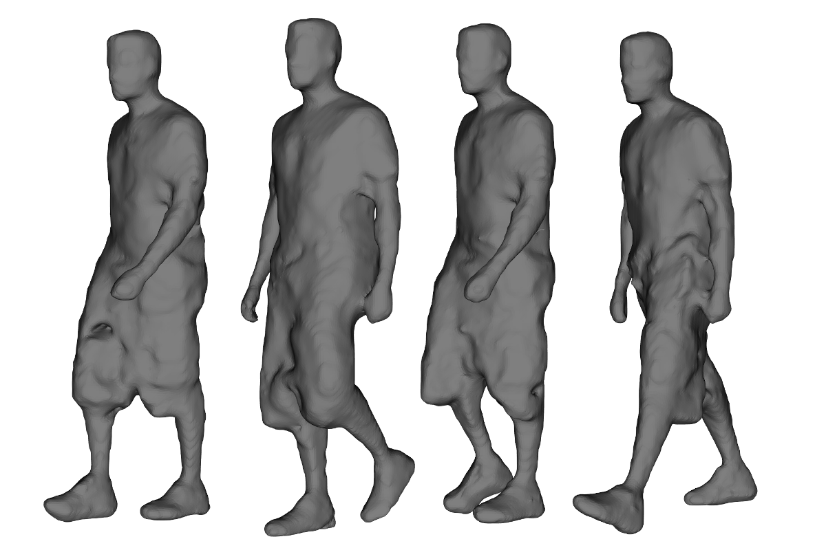
  Fig. 4: Walking motion from CVSSP3D dataset

  As the reader can see in Figure 4, some of the motions in this dataset represent humans moving in loose-fitting clothes. The sensitivity of the reconstructed surface to clothes induces presence of noise in the meshes (see Figure 8) which makes it a challenge for 3D human motion retrieval.

• Synthetic dataset. A synthetic model (1290 vertices and 2108 faces) is animated thanks to real motion skeleton data. Fourteen individuals performed each 28 different motions: sneak, walk (slow, fast, turn left/right, circle left/right, cool, cowboy, elderly, tired, macho, march, mickey, sexy, dainty), run (slow, fast, turn right/left, circle left/right), sprint, vogue, faint, rock n’roll, shoot. It has already been used [19] for static shape evaluation in the context of 3D motion analysis. A motion from this dataset is presented in Figure 5. The sampling of the sequences is set to 25Hz.

  

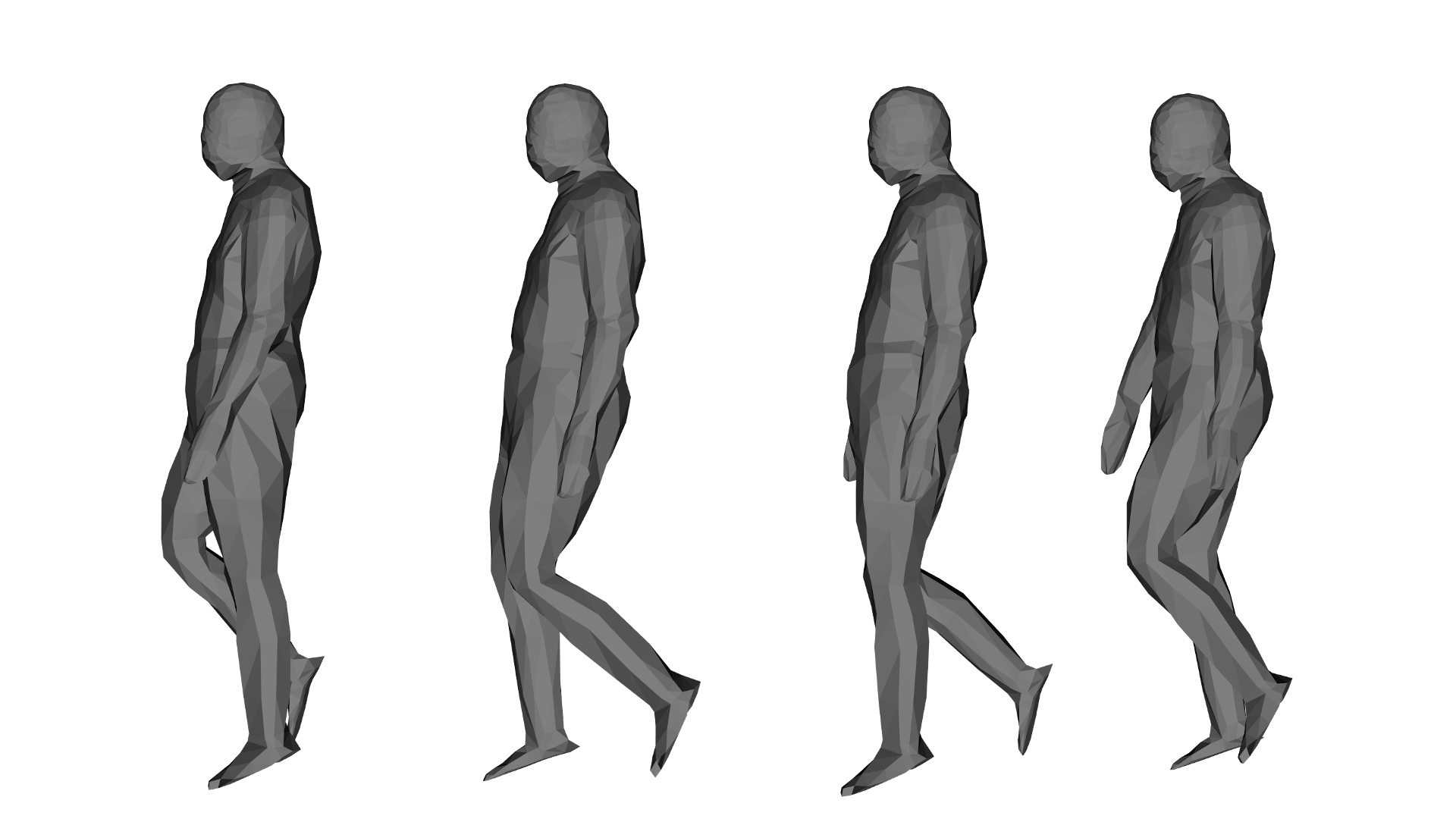
  Fig. 5: Slow walking motion from CVSSP3D synthetic dataset

4.3 Static pose retrieval on the FAUST dataset

Fig. 6: Overview of our pose retrieval approach: We first compute the descriptors (Areas/Breadths or Areas & Breadths) of all shapes in the database. Given a query shape, we compute its corresponding descriptor and collect the closest shapes in the descriptor space.

Each pose of a dataset is considered as a query belonging to some class. We compute the Euclidean distance between the query pose descriptors and each pose in the dataset (Figure  6).

Comparison with state-of-the-art. In order to evaluate our descriptor against available methods in the literature, we compare to the following approaches:

1. Skinned Multi-Person Linear model (SMPL) pose representation. The SMPL body model [30] is composed of three parts: a template mesh, a pose vector, and a shape vector. The shape vector represents the (non-rigid) deformation of the template to the shape of the given human body. The pose information of a skeletal joint is the relative rotation of the joint of the skeleton compared to its parent joint, and is stored either as the rotation matrix or as axis-angle representation. We convert each joint rotation to quaternion representation as in [17, 16] and measure the distance between unit quaternions by $d(q,q^{\prime})=1-|q.q^{\prime}|$. The SMPL body pose vector contains the pose information of 52 joints, and the rotation of the central joint accounts for the global rotation of the shape. The representation is a point in $(\mathbb{R}^{4})^{51}=\mathbb{R}^{204}$. Due to the construction of the pose vector, this descriptor is rotation invariant. However, this method is time consuming compared to ours because of the needed fitting operation to the mesh.

2. Aumentado-Armstrong et al. [16] propose Geometrically Disentangled VAE (GDVAE), a point cloud variational autoencoder which is trained to disantengle the intrinsic and extrinsic informations of a given shape in the latent space. The authors propose the intrinsic and extrinsic latent vectors for human shape representation. We used the FAUST meshes as input of their available trained network, gathered their extrinsic latent vectors (belonging to $\mathbb{R}^{12}$), and used them for human pose retrieval. Although the procedure is parametrization invariant by nature (the networks takes a cloud of points as input), the training uses the mesh Laplacian as ground truth information, and this means a constant parameterization along the training set. The network is trained on the SURREAL dataset [31] in such a way as to be rotation invariant.

3. Zhou et al. [17] propose a mesh autoencoder based on the Neural3DMM [32] graph neural network structure. As in the case of GDVAE, this autoencoder disantengles shape and pose in latent space. The network requires that all input meshes have the same parameterization. We apply the FAUST meshes on their available network trained on the AMASS dataset, and use the pose latent vector (belonging to $\mathbb{R}^{112}$) as a descriptor for comparison. Since the input of the network are the coordinates of the vertices, the approach is not rotation invariant.

Representation	NN	FT	ST
Areas	62	50.0	67.2
Breadths	83	63.1	76.6
Areas & Breadths	86	67.9	80.9
GDVAE [16]	60	38.0	54.2
Zhou et al. [17]	82	69.2	83.4
SMPL pose vector	80	84.4	95.2

Table 2: Results on pose retrieval for FAUST dataset .

Representation	Computation time
Areas	4.1ms
Breadths	13.2ms
Areas & Breadths	17.2ms
GDVAE [16]	190ms
Zhou et al. [17]	30.7ms
SMPL pose vector	$\approx 5min$

Table 3: Computation time for feature extraction for each method on the FAUST dataset. The computations were performed with NumPy routines on a Intel(R) Core(TM) i5-7600K 3.8GHz CPU, with 8GB of RAM available, except for SMPL, for which the given method needed the use of a GPU.

Table 2 displays the results obtained for the Areas, Breadths, and Areas & Breaths descriptors. The results for the Breadths descriptor is of particular interest as it is here where we see the high correlation between poses and their (symmetrized) convex hull, which validates our main hypothesis. In fact, Breadth by itself outperforms all previous methods in the NN criterion. When complemented by areas, the performance improves by $3\%$. The results also show that the SMPL pose vector performs much better for the FT and ST metrics. This result can be explained by the fact that SMPL has been designed specifically for human shapes. In addition, the SMPL fitting method used here requires a dataset of meshes registered to a template. The Table 3 shows that our approach is faster than all the methods. It shows also that the computation time of SMPL descriptor is very high.

4.4 3D Human Motion retrieval on CVSSP3D artificial dataset

Fig. 7: Overview of our motion retrieval approach. We first compute the time series of descriptors (areas/breadth spectra or shape invariant) of all motions in the database. Given a query shape, we compute its corresponding time series and compare it against the time series of the database in the descriptor space using dynamic time warping. We then collect the closest motions given this similarity

Each mesh sequence of a dataset is considered as a query belonging to some class. We compute the DTW similarity between the query mesh sequence and each mesh sequence in the dataset (Figure  7).

Comparison with state-of-the-art. An extensive comparison has been made in [22] to evaluate a bench of descriptors for human motion retrieval. The polygonal curves of those descriptors are filtered with a temporal filtering approach(a mean filter is applied along a temporal window of size $K$). Finally, the dynamic time warping distance is used for comparing the resulting curves. We compare our invariant descriptors (breadth and area spectrum, shape invariant) to the euclidean and parameterization invariant features presented in [22], which are:

1. Shape Distribution [33][22] is a 3D descriptor based on pairwise distances. All pairwise distances of a given shape are computed, and the resulting descriptor is an histogram of the obtained distances.

2. Spin Images [34][22] is a 3D shape descriptor based on local features. For each point of a shape, a view from the point (the spin image) is computed, which takes the form of a 2D histogram. The resulting descriptor is the sum of all spin images.

3. The pretrained GDVAE on SURREAL is applied directly on the dataset. It does not need any supplementary work since the network (PointNet) is parameterization invariant.

4. The Neural3DMM autoencoder from [17] needs to be specifically trained on the CVSSP3D artificial dataset, since the network is set to specific mesh parameterization and alignment. In order to be fair to the other methods that were not trained on the dataset, we apply a cross identity validation to compute the score. For each individual, we remove its motions from the training dataset. We then compute the retrieval scores for the individual motions using the trained pose representation. The training setting is exactly the same as in [17].

Representation	NN	FT	ST
Area spectrum	81.6	56.6	68.2
Breadth spectrum	100	99.8	100
Shape invariant $\mathcal{E}^{s}_{7}$	82.1	56.8	68.5
Shape Distribution [35][22]	92.1	88.9	97.2
Spin Images [34][22]	100	87.1	94.1
GDVAE [16]	100	97.6	98.8
Zhou et al. [17]	100	99.6	99.6

Table 4: CVSSP3D artificial dataset results for motion retrieval using our shape-invariant representations. The results of Shape Distributions and Spin Images are reported from [22].

We report our results on CVSSP3D artificial dataset in Table 4. The window sizes for temporal filtering applied to Shape Distribution and Spin Images are 9 and 8 respectively as in [22]. Our method did not require temporal filtering. We observe that the breadth spectrum has the best performance, near $100\%$, in all criteria.

4.5 3D Human Motion retrieval on CVSSP3D Real Dataset

The CVSSP3D real dataset differs significantly from the artificial human motion dataset because of the relatively noisy data (see Figure 8) and the various kinds of loose-fitting clothes in some of the models (see Figure 4 and Table 6).

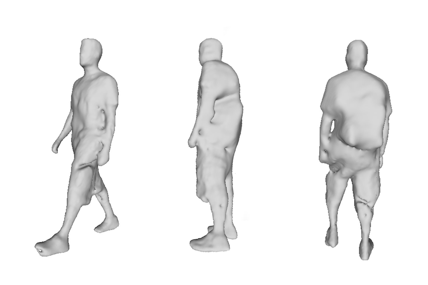
Fig. 8: Examples of artifacts in the CVSSP3D real dataset.

This raises the problem of making our descriptors more robust. While a thorough study of this question will be left for a future publication, two conceptually simple and easily implemented modifications to our method can have a significant impact.

The $\lambda$-percentile breadth function.

The breadth function is particularly sensitive to outliers: the maximum or the minimum value of the function $x\mapsto u\cdot x$ can change significantly with a single noisy vertex $x$. To make this descriptor more robust we make a simple change to the support function of a finite set:

Definition 4.1

Given a finite set $S\subset{\mathbb{R}}^{n}$ and a parameter $\lambda$, $0<\lambda\leq 100$, we define the $\lambda$-percentile support function of $S$ as the function $h_{\lambda}(S,\cdot)$ that assigns to a unit vector $u\in S^{n-1}$ the $\lambda$-th percentile of the values $\{u\cdot x:x\in S\}$. The $\lambda$-percentile breadth function of $S$ is given by

$$b_{\lambda}(M;u)=h_{\lambda}(S;u)+h_{\lambda}(S;-u).$$

Defined in terms of the vertices of a triangulation, $b_{\lambda}(M;\cdot)$ is not invariant under re-triangulations of the surface for $\lambda<100$. It is only approximately so if the mesh is fine enough and the sizes and shapes of all triangles are comparable. Nevertheless, it is invariant under translations of $M$ and satisfies the equivariance condition

$$b_{\lambda}(RM;u)=b_{\lambda}(M;R^{-1}u).$$

Provided we understand the conditions on the meshes of the surfaces we are working with, we can use $b_{\lambda}(M;\cdot)$ as a substitute of the breadth function in the construction of shape invariants detailed in Section 3.3. We experimented with various values for $\lambda$ and settled on the classic third quartile $\lambda=75$. We call the function $b_{75}(M;u)$ Q-breadth. The analogue of the shape-invariant $\mathcal{E}^{s}_{8}$ computed with the Q-breadth function instead of the breadth function will be called the Q-shape invariant.

Temporal filtering

Our second trick consists in slightly changing the way we assign polygonal curves to sequences of surfaces with timestamps by making use of a special feature of our invariants. If we are given a sequence of surfaces we can consider their average breadth function and their average weighted area function, and then proceed with the construction of the feature vectors. Note that for the breadth spectrum, the area spectrum and the shape invariant this is not the same as averaging the feature vectors themselves (we tried that too: the results were not as good). This particularity of our representation allows us the possibility to perform a simple discrete convolution or temporal filtering on the data: given a sequence of surfaces with timestamps, $(M_{0},t_{0}),\ldots,(M_{p},t_{p})$ and a number $K$, $0<K<p$ we consider the timestamped averages of breadth and weighted area functions, which are both represented here by $f$ to avoid redundancy,

$$\bar{f}_{t_{i}}(M;u):=\frac{1}{2K+1}\sum_{-K\leq j\leq K}f(M_{i+j};u),\ K\leq i\leq p-K.$$

With the sequence of timestamped averaged functions

$$\bar{f}_{t_{K}}(M;u),\ldots,\bar{f}_{t_{p-K}}(M;u)$$

we construct our timestamped feature vectors and the corresponding polygonal curve as described in Section 3.5. Note that this temporal filtering approach is slightly different from the one proposed in [22] – our approach is using the specific structure of our descriptors. The results of our experiments and comparisons on the CVSSP3D real dataset are reported in Table 5. Again we report the results of Shape distances and Spin Images from [22]. We display in this table the used windows size for temporal filtering of each method. For this relatively noisy dataset, the table clearly shows the advantage of using the spectrum of the Q-breadth function and the Q-shape invariant.

The results in Table 5 show that the Q-shape invariant outperforms all other methods, including the deep learning method GDVAE whose performance drops significantly in the presence of noise. This can be explained by the noise-sensitivity of the spectrum of the Laplace-Beltrami Operator.

A remarkable difference between the results in Table 5 and those of Table 4 is that the first tier measure is quite low compared to the NN measure for all features. In order to give an idea of how the tier are distributed, a first tier query is illustrated in Table 6.

Repr.	$K$	NN	FT	ST
Area spectrum	14	67.5	47.0	63.2
Breadth spectrum	15	63.7	39.1	52.5
Q-breadth spectrum	5	80.0	44.8	59.5
Shape invariant $\mathcal{E}^{s}_{7}$	15	62.5	41.8	57.9
Q-shape invariant	4	82.5	51.3	68.8
Shape Distribution [35]	1	77.5	51.6	65.5
Spin Images [34]	6	66.3	43.2	59.5
GDVAE [16]	14	38.7	31.6	51.6

Table 5: CVSSP3D real dataset results for motion retrieval using our shape-invariant representations and their Q-versions. The results of Shape Distributions and Spin Images are reported from [22]. The K value is the best window size for temporal filtering, and the displayed score are the corresponding best scores.

Motion	Picture
Nikos, Walk (Query)
Jean, Walk
Jon, Walk
Hansung Walk
Chris, Walk
Haidi, Walk
Hansung, Walk, Run and Jump
Nikos, Run

Table 6: First seven results of a query on the CVSSP3D real dataset using the Q-shape invariant as our representation.

4.6 Computation times

Our methods were implemented using Numpy routines, with no other optimization. The computations were performed with NumPy routines on a Intel(R) Core(TM) i5-7600K 3.8GHz CPU, with 8GB of RAM available.

In Table 3 we present the computation of each method. For Zhou et al. [17] and Aumentado-Armstrong et al. [16], we used the implementation, provided by the authors. For SMPL, we used the SMPL fitting pipeline proposed by the authors. In Table 7 we present the computation time of each method for the CVSSP3D datasets. For Zhou et al. [17] and Aumentado-Armstrong et al. [16] (GDVAE) we used the implementation provided by the authors. For Shape Distribution we use the hybrid Python-C implementation provided by Nenad Markuš . For Spin Images, we used the C++ implementation provided by the PointCloud library . We can see that our approach is the fastest on FAUST and CVSSP3D artificial datasets. We observe that the Q-shape invariant computation time is a bit slower than Shape Distribution for our approach in the real dataset – but the performance of our approach improves the NN criteria by 5%.

Method	Real, 37800 vert.	Artif., 1290 vert.
Shape Dist.	79.1s*	61.2s*
Spin Image	3h54*	35.7s*
GDVAE	56.4s	2.08s
Shape invariant $\mathcal{E}^{s}_{7}$	46s	1.7s
Q-shape invariant	209s	/

Table 7: Mean computation time of polygonal curves extraction for different methods in the CVSSP3D datasets, along with the time corresponding to the polygonal curves in ${\mathbb{R}}^{24}$ using the Shape invariant $\mathcal{E}^{s}_{7}$, and the Q-shape invariant. We put the number of vertices for each dataset. Methods with an asterisk means that the implementation is not the official implementation provided by the authors.

5 Conclusion and Future Work

5.1 Conclusion

We defined a novel human descriptors using purely geometric information. Our approach is based on the intuition that a human pose is nearly characterized by its convex hull. Based on this hypothesis, we introduced three sequences of numerical surface descriptors that are invariant under reparametrizations, Euclidean transformations and similarities. We demonstrated the use of these descriptors by performing pose retrieval and extending their use to human motion retrieval. Our experiments on the FAUST and CVSSP3D synthetic and real datasets demonstrated that our method generally outperforms the state-art-methods for both 3D human pose and motion retrieval including deep learning approaches.

5.2 Future Work

Several avenues of future work are worth pursuing. We list some most promising directions below:

• A first question is to ask if other descriptors [36, 37] of convex shapes with similar property as CH or EGI are suitable for describing the human pose.

• The noisy CVSSP3D real dataset has been a challenge for our descriptors. Some research should be spent on a statistical analysis as in in [38] to improve performance on noisy data.

• As can be seen in Table 4, the fusion of several descriptors does not automatically lead to better results. A finer statistical analysis is needed to exploit the existence of different descriptors.

• It would be interesting to apply the geometric invariant and easily-computable descriptors proposed in this paper in a geometric deep learning approaches [18].

6 Acknowledgments

This work was supported by the ANR project Human4D ANR-19-CE23-0020. This work was also partially supported by the French State, managed by National Agency for Research (ANR) under the Investments for the future program with reference ANR-16-IDEX-0004 ULNE.

References

- Tumpach et al. [2016] Tumpach, AB, Drira, H, Daoudi, M, Srivastava, A. Gauge invariant framework for shape analysis of surfaces. IEEE Trans Pattern Anal Mach Intell 2016;38(1):46–59.
- Kurtek et al. [2012] Kurtek, S, Klassen, E, Gore, JC, Ding, Z, Srivastava, A. Elastic geodesic paths in shape space of parameterized surfaces. IEEE Trans Pattern Anal Mach Intell 2012;34(9):1717–1730.
- Jermyn et al. [2012] Jermyn, IH, Kurtek, S, Klassen, E, Srivastava, A. Elastic shape matching of parameterized surfaces using square root normal fields. In: Fitzgibbon, A, Lazebnik, S, Perona, P, Sato, Y, Schmid, C, editors. Computer Vision – ECCV 2012. Berlin, Heidelberg: Springer Berlin Heidelberg; 2012, p. 804–817.
- Kaula [1967] Kaula, WM. Theory of statistical analysis of data distributed over a sphere. Reviews of Geophysics 1967;5(1):83–107.
- Lowes [1974] Lowes, FJ. Spatial Power Spectrum of the Main Geomagnetic Field, and Extrapolation to the Core. Geophysical Journal International 1974;36(3):717–730.
- Kazhdan et al. [2003] Kazhdan, MM, Funkhouser, TA, Rusinkiewicz, S. Rotation invariant spherical harmonic representation of 3D shape descriptors. In: Kobbelt, L, Schröder, P, Hoppe, H, editors. First Eurographics Symposium on Geometry Processing, Aachen, Germany, June 23-25, 2003; vol. 43 of ACM International Conference Proceeding Series. Eurographics Association; 2003, p. 156–164.
- Starck and Hilton [2007] Starck, J, Hilton, A. Surface capture for performance-based animation. IEEE Computer Graphics and Applications 2007;27(3):21–31.
- Pickup et al. [2016] Pickup, D, Sun, X, Rosin, PL, Martin, RR, Cheng, Z, Lian, Z, et al. Shape Retrieval of Non-rigid 3D Human Models. International Journal of Computer Vision 2016;120(2):169–193.
- Osada et al. [2001] Osada, R, Funkhouser, T, Chazelle, B, Dobkin, D. Matching 3D models with shape distributions. In: Proceedings International Conference on Shape Modeling and Applications. 2001, p. 154–166. doi:10.1109/SMA.2001.923386.
- Horn [1984] Horn, B. Extended gaussian images. Proceedings of the IEEE 1984;72(12):1671–1686. doi:10.1109/PROC.1984.13073.
- Ankerst et al. [1999] Ankerst, M, Kastenmüller, G, Kriegel, H, Seidl, T. 3D shape histograms for similarity search and classification in spatial databases. In: Güting, RH, Papadias, D, Lochovsky, FH, editors. Advances in Spatial Databases, 6th International Symposium, SSD’99, Hong Kong, China, July 20-23, 1999, Proceedings; vol. 1651 of Lecture Notes in Computer Science. Springer; 1999, p. 207–226.
- Sun et al. [2009] Sun, J, Ovsjanikov, M, Guibas, LJ. A concise and provably informative multi-scale signature based on heat diffusion. Comput Graph Forum 2009;28(5):1383–1392.
- Bronstein and Kokkinos [2010] Bronstein, MM, Kokkinos, I. Scale-invariant heat kernel signatures for non-rigid shape recognition. In: 2010 IEEE Computer Society Conference on Computer Vision and Pattern Recognition. 2010, p. 1704–1711.
- Aubry et al. [2011] Aubry, M, Schlickewei, U, Cremers, D. The wave kernel signature: A quantum mechanical approach to shape analysis. In: 2011 IEEE International Conference on Computer Vision Workshops (ICCV Workshops). 2011, p. 1626–1633.
- Reuter et al. [2006] Reuter, M, Wolter, F, Peinecke, N. Laplace-beltrami spectra as ’shape-dna’ of surfaces and solids. Comput Aided Des 2006;38(4):342–366.
- Aumentado-Armstrong et al. [2019] Aumentado-Armstrong, T, Tsogkas, S, Jepson, A, Dickinson, S. Geometric disentanglement for generative latent shape models. In: 2019 IEEE/CVF International Conference on Computer Vision (ICCV). 2019, p. 8180–8189.
- Zhou et al. [2020] Zhou, K, Bhatnagar, BL, Pons-Moll, G. Unsupervised shape and pose disentanglement for 3D meshes. In: Vedaldi, A, Bischof, H, Brox, T, Frahm, JM, editors. Computer Vision – ECCV 2020. Cham; 2020, p. 341–357.
- Bronstein et al. [2017] Bronstein, MM, Bruna, J, LeCun, Y, Szlam, A, Vandergheynst, P. Geometric deep learning: going beyond euclidean data. IEEE Signal Processing Magazine 2017;34(4):18–42.
- Huang et al. [2010] Huang, P, Hilton, A, Starck, J. Shape similarity for 3D video sequences of people. International Journal of Computer Vision 2010;89(2-3):362–381.
- Slama et al. [2014] Slama, R, Wannous, H, Daoudi, M. 3D human motion analysis framework for shape similarity and retrieval. Image and Vision Computing 2014;32(2):131–154.
- Luo et al. [2016] Luo, G, Cordier, F, Seo, H. Spatio-temporal segmentation for the similarity measurement of deforming meshes. The Visual Computer 2016;32(2):243–256.
- Veinidis et al. [2019] Veinidis, C, Danelakis, A, Pratikakis, I, Theoharis, T. Effective descriptors for human action retrieval from 3D mesh sequences. Int J Image Graph 2019;19(3):1950018:1–1950018:34.
- Choquet [1969] Choquet, G. Lectures on Analysis; vol. 3. Reading, Massachusetts: W.A. Benjamin, Inc.; 1969.
- Arnold [2004] Arnold, V. Lectures on Partial Differential Equations. Universitext; Berlin Heidelberg and Moscow: Springer-Verlag and PHASIS; 2004.
- Weyl [1946] Weyl, H. The classical groups. Princeton, NJ: Princeton University Press; 1946.
- Santaló [1976] Santaló, L. Integral geometry and geometric probability; vol. 1 of Encyclopedia of Mathematics and its Applications. Reading, Mass.-London-Amsterdam: Addison-Wesley Publishing Co; 1976.
- Wieczorek and Meschede [2018] Wieczorek, MA, Meschede, M. Shtools: Tools for working with spherical harmonics. Geochemistry, Geophysics, Geosystems 2018;19(8):2574–2592.
- Livermore [2012] Livermore, PW. The Spherical Harmonic Spectrum of a Function with Algebraic Singularities. Journal of Fourier Analysis and Applications 2012;18(6):1146–1166.
- Bogo et al. [2014] Bogo, F, Romero, J, Loper, M, Black, MJ. FAUST: Dataset and evaluation for 3D mesh registration. In: 2014 IEEE Conference on Computer Vision and Pattern Recognition. 2014, p. 3794–3801.
- Loper et al. [2015] Loper, M, Mahmood, N, Romero, J, Pons-Moll, G, Black, MJ. SMPL: A skinned multi-person linear model. ACM Trans Graphics (Proc SIGGRAPH Asia) 2015;34(6):248:1–248:16.
- Varol et al. [2017] Varol, G, Romero, J, Martin, X, Mahmood, N, Black, MJ, Laptev, I, et al. Learning from synthetic humans. In: 2017 IEEE Conference on Computer Vision and Pattern Recognition, CVPR 2017, Honolulu, HI, USA, July 21-26, 2017. IEEE Computer Society; 2017, p. 4627–4635.
- Bouritsas et al. [2019] Bouritsas, G, Bokhnyak, S, Ploumpis, S, Zafeiriou, S, Bronstein, MM. Neural 3D morphable models: Spiral convolutional networks for 3D shape representation learning and generation. In: 2019 IEEE/CVF International Conference on Computer Vision, ICCV 2019, Seoul, Korea (South), October 27 - November 2, 2019. IEEE; 2019, p. 7212–7221.
- Osada et al. [2002a] Osada, R, Funkhouser, TA, Chazelle, B, Dobkin, DP. Shape distributions. ACM Trans Graph 2002a;21(4):807–832.
- Johnson and Hebert [1999] Johnson, AE, Hebert, M. Using spin images for efficient object recognition in cluttered 3D scenes. IEEE Trans Pattern Anal Mach Intell 1999;21(5):433–449.
- Osada et al. [2002b] Osada, R, Funkhouser, TA, Chazelle, B, Dobkin, DP. Shape distributions. ACM Trans Graph 2002b;21(4):807–832.
- Engel and Laasch [2020] Engel, K, Laasch, B. Reconstruction of polytopes from the modulus of the Fourier transform with small wave length. arXiv preprint arXiv:201106971 2020;.
- Kousholt and Schulte [2021] Kousholt, A, Schulte, J. Reconstruction of Convex Bodies from Moments. Discrete & Computational Geometry 2021;65(1):1–42.
- Poonawala et al. [2002] Poonawala, A, Milanfar, P, Gardner, R. A statistical analysis of shape reconstruction from areas of shadows. In: Conference Record of the Thirty-Sixth Asilomar Conference on Signals, Systems and Computers, 2002.; vol. 1. Pacific Grove, CA, USA: IEEE; 2002, p. 916–920.