KCL-MTH-21-02


Free fermions, KdV charges, generalised Gibbs ensembles and modular transforms
Max Downing and Gérard M.T. Watts

Department of Mathematics, King’s College London,

Strand, London WC2R 2LS, UK


Abstract

In this paper we consider the modular properties of generalised Gibbs ensembles in the Ising model, realised as a theory of one free massless fermion. The Gibbs ensembles are given by adding chemical potentials to chiral charges corresponding to the KdV conserved quantities. (They can also be thought of as simple models for extended characters for the W-algebras). The eigenvalues and Gibbs ensembles for the charges can be easily calculated exactly using their expression as bilinears in the fermion fields. We re-derive the constant term in the charges, previously found by zeta-function regularisation, from modular properties. We expand the Gibbs ensembles as a power series in the chemical potentials and find the modular properties of the corresponding expectation values of polynomials of KdV charges. This leads us to an asymptotic expansion of the Gibbs ensemble calculated in the opposite channel. We obtain the same asymptotic expansion using Dijkgraaf’s results for chiral partition functions. By considering the corresponding TBA calculation, we are led to a conjecture for the exact closed-form expression of the GGE in the opposite channel. This has the form of a trace over multiple copies of the fermion Fock space. We give analytic and numerical evidence supporting our conjecture.

1 Introduction

Two-dimensional conformal field theories have been known for a long time to have an infinite set of commuting conserved charges. There is always an infinite set of local charges composed entirely from modes of the Virasoro algebra that we call “KdV charges” for their equivalence to the charges in the KdV hierarchy [1, 2]. There is an independent infinite set of charges related to the ZMS-Bullough-Dodd model, see for example [3], as well as further (different) sets of charges if the conformal field theory has an extended chiral (W-algebra) symmetry. Most recently, such charges have played a key role in the understanding of non-thermal or Generalised Gibbs ensembles (GGEs) [4, 5], and the extension of the local charges to so-called quasi-local charges [6]. These GGEs have already been studied in the large central charge limit in [7, 8].

One obvious question is that of the modular properties of a GGE. The idea of modular invariance of the standard partition function on the torus, the invariance under reparametrisations of the torus, was central to the understanding of conformal field theory and much of the classification work rests on this. The question is: what are the modular properties of the partition function of a GGE?

Independently, there has also been interest in (extended) characters of W-algebras, both for their relevance for descriptions of Black Holes [9, 10] and in their own right [11]. A W-algebra is a set of generating fields amongst which one can find a subset whose zero modes $\{W^{i}_{0}\}$ commute. It is a natural idea to consider the character encoding the dimensions of eigenspaces of these zero modes. The “standard” character includes only one of the other generators, $L_{0}$ and its known in certain circumstances to have well-defined modular properties, and there has been a natural desire to understand “extended” characters including the full set $\{W^{i}_{0}\}$, both from mathematical and physical considerations. It is to be expected that this problem shares many of the issues of the GGE and this was in fact one of the main motivations of this paper, even if the fields in this model do not actually form a W-algebra.

In this paper we look in detail at the simplest case, that of the KdV charges in the Ising model, or equivalently, the theory of a single free fermion. In this model the charges are diagonal on the fermion creation modes and so it is easy to give an explicit formula for the GGE partition function. We first give the general setting of the GGE in section 2. We then describe the free fermion model, its conserved charges and the construction of the GGE partition function in section 3. We then investigate its modular properties in two ways: a direct investigation of the GGE partition function formula in section 4 and through Dijkgraaf’s much earlier work on Chiral deformations of conformal field theories in section 5. We arrive at the same results by these two methods, that the modular transform of a GGE partition function composed of local charges does not have a convergent expression as a GGE partition function composed of local charges. Instead, we find an expression for the modular transform that is asymptotically correct, and conjecture a convergent formula for the ground-state contribution.

We also check the modular properties of the expressions we have found against the modular differential equation results of [12].

We then investigate the same system through the thermodynamic Bethe ansatz (TBA) in section 6. We find the same expression for the ground state contribution that we conjectured before, but a richer set of possible excited state energies. These include the energies found in the previous sections but with two further sets which give a correction to the partition function with vanishing asymptotic expansion. This leads to a conjectural formula for the modular transform of the partition function that includes all sets of “excited state” poles from TBA. In section 7 we test this conjecture numerically in the simplest case and find agreement (within numerical accuracy).

In section 8, we finish with some observations on this formula, its possible proof, interpretation and extensions.

2 GGEs

The general setting is of a conformal field theory defined on a circle of circumference $R$, with Hamiltonian $H(R)$ and momentum operator $P(R)$. We consider the generalised partition function on a cylinder of length $L$,

$$Z(L,R,a)={\mathrm{Tr}}(e^{-LH(R)}e^{iaP(R)})\;,$$ (2.1)

where we have inserted a rotation through a distance $a$ around the cylinder. This can be calculated as the partition function on the cylinder where the ends are identified up to a translation at one end, as in figure 1(a).

uvwzRLa=LRaAARLa1τ1q(a)(b)(c)(d)(e)missing-subexpressionmissing-subexpressionumissing-subexpressionvmissing-subexpressionwmissing-subexpressionzmissing-subexpression𝑅𝐿𝑎𝐿𝑅𝑎𝐴superscript𝐴𝑅𝐿𝑎1𝜏1𝑞missing-subexpression𝑎missing-subexpression𝑏missing-subexpression𝑐missing-subexpression𝑑missing-subexpression𝑒missing-subexpression\begin{array}[]{cccccccccc}&&\hfill\mbox{\Large$\llcorner$}\raisebox{2.84526pt}{\kern-3.98337pt{$u$}}&&\hfill\mbox{\Large$\llcorner$}\raisebox{2.84526pt}{\kern-3.98337pt{$v$}}&&\hfill\mbox{\Large$\llcorner$}\raisebox{2.84526pt}{\kern-3.98337pt{$w$}}&&\hfill\mbox{\Large$\llcorner$}\raisebox{2.84526pt}{\kern-3.98337pt{$z$}}\\[-8.53581pt] \leavevmode\hbox to91.01pt{\vbox to52.75pt{\pgfpicture\makeatletter\hbox{\hskip 27.55858pt\lower-1.59998pt\hbox to0.0pt{\pgfsys@beginscope\pgfsys@invoke{ }\definecolor{pgfstrokecolor}{rgb}{0,0,0}\pgfsys@color@rgb@stroke{0}{0}{0}\pgfsys@invoke{ }\pgfsys@color@rgb@fill{0}{0}{0}\pgfsys@invoke{ }\pgfsys@setlinewidth{0.4pt}\pgfsys@invoke{ }\nullfont\pgfsys@beginscope\pgfsys@invoke{ }\pgfsys@invoke{\lxSVG@closescope }\pgfsys@endscope\hbox to0.0pt{\pgfsys@beginscope\pgfsys@invoke{ } \pgfsys@beginscope\pgfsys@invoke{ }{{}} {}{{}}{} {}{}{}\pgfsys@moveto{0.0pt}{19.69048pt}\pgfsys@lineto{56.90552pt}{19.69048pt}\pgfsys@stroke\pgfsys@invoke{ } {}{{}}{} {}{}{}\pgfsys@moveto{0.0pt}{48.14323pt}\pgfsys@lineto{56.90552pt}{48.14323pt}\pgfsys@stroke\pgfsys@invoke{ } {}{{}}{}{{{}} {}{}{}{}{}{}{}{}}{}\pgfsys@moveto{0.0pt}{33.91685pt}\pgfsys@moveto{5.69046pt}{33.91685pt}\pgfsys@curveto{5.69046pt}{41.77396pt}{3.14279pt}{48.14323pt}{0.0pt}{48.14323pt}\pgfsys@curveto{-3.14279pt}{48.14323pt}{-5.69046pt}{41.77396pt}{-5.69046pt}{33.91685pt}\pgfsys@curveto{-5.69046pt}{26.05975pt}{-3.14279pt}{19.69048pt}{0.0pt}{19.69048pt}\pgfsys@curveto{3.14279pt}{19.69048pt}{5.69046pt}{26.05975pt}{5.69046pt}{33.91685pt}\pgfsys@closepath\pgfsys@moveto{0.0pt}{33.91685pt}\pgfsys@stroke\pgfsys@invoke{ } {}{{}}{}{{}{}{}{{}}{{{{}{}{}{}}} {{}{}{}{}}}}{} {} {} {} {}{}{}\pgfsys@moveto{56.90552pt}{19.69048pt}\pgfsys@curveto{60.04831pt}{19.69048pt}{62.59598pt}{26.05975pt}{62.59598pt}{33.91685pt}\pgfsys@curveto{62.59598pt}{41.77396pt}{60.04831pt}{48.14323pt}{56.90552pt}{48.14323pt}\pgfsys@stroke\pgfsys@invoke{ } {}{{}}{}{{}{}{}{{}}{{{{}{}{}{}}} {{}{}{}{}}}}{} {} {} {} {}{}\pgfsys@beginscope\pgfsys@invoke{ }\pgfsys@setdash{3.0pt,3.0pt}{0.0pt}\pgfsys@invoke{ }{}\pgfsys@moveto{56.90552pt}{48.14323pt}\pgfsys@curveto{53.76273pt}{48.14323pt}{51.21506pt}{41.77396pt}{51.21506pt}{33.91685pt}\pgfsys@curveto{51.21506pt}{26.05975pt}{53.76273pt}{19.69048pt}{56.90552pt}{19.69048pt}\pgfsys@stroke\pgfsys@invoke{ } \pgfsys@invoke{\lxSVG@closescope }\pgfsys@endscope{}{{}}{}{{}{}{}{{}}{{{{}{}{}{}}} {{{}{}{}{}}} {{}{}{}{}}}}{} {} {} {} {}{}{{}}{}{{ {\pgfsys@beginscope\pgfsys@setlinewidth{0.32pt}\pgfsys@setdash{}{0.0pt}\pgfsys@roundcap\pgfsys@roundjoin{} {}{}{} {}{}{} \pgfsys@moveto{-1.19998pt}{1.59998pt}\pgfsys@curveto{-1.09998pt}{0.99998pt}{0.0pt}{0.09999pt}{0.29999pt}{0.0pt}\pgfsys@curveto{0.0pt}{-0.09999pt}{-1.09998pt}{-0.99998pt}{-1.19998pt}{-1.59998pt}\pgfsys@stroke\pgfsys@endscope}} }{}{}{{}}\pgfsys@moveto{-13.6572pt}{23.95865pt}\pgfsys@curveto{-11.47978pt}{20.81595pt}{-8.69545pt}{22.68105pt}{-7.43832pt}{28.12437pt}\pgfsys@curveto{-6.1812pt}{33.5677pt}{-6.92726pt}{40.52832pt}{-9.10468pt}{43.67102pt}\pgfsys@curveto{-11.28209pt}{46.81372pt}{-14.06642pt}{44.94862pt}{-15.22005pt}{39.95348pt}\pgfsys@stroke\pgfsys@invoke{ }{{}{{}}{}{}{{}}{{{}}{{{}}{\pgfsys@beginscope\pgfsys@invoke{ }\pgfsys@transformcm{-0.22504}{-0.97435}{0.97435}{-0.22504}{-15.22003pt}{39.95349pt}\pgfsys@invoke{ }\pgfsys@invoke{ \lxSVG@closescope }\pgfsys@invoke{\lxSVG@closescope }\pgfsys@endscope}}{{}}}}\hbox{\hbox{{\pgfsys@beginscope\pgfsys@invoke{ }{{}{}{{ }}{ } {{}{{}}}{{}{}}{}{{}{}} { }{{{{}}\pgfsys@beginscope\pgfsys@invoke{ }\pgfsys@transformcm{1.0}{0.0}{0.0}{1.0}{-24.22557pt}{43.03828pt}\pgfsys@invoke{ }\hbox{{\definecolor{pgfstrokecolor}{rgb}{0,0,0}\pgfsys@color@rgb@stroke{0}{0}{0}\pgfsys@invoke{ }\pgfsys@color@rgb@fill{0}{0}{0}\pgfsys@invoke{ }\hbox{{$\scriptstyle R$}} }}\pgfsys@invoke{\lxSVG@closescope }\pgfsys@endscope}}} \pgfsys@invoke{\lxSVG@closescope }\pgfsys@endscope}}} {}{{}}{} {}{}\pgfsys@beginscope\pgfsys@invoke{ }\pgfsys@setdash{3.0pt,3.0pt}{0.0pt}\pgfsys@invoke{ }{}{}{}{}{{}}{}{}{}{{}}\pgfsys@moveto{0.45999pt}{14.00002pt}\pgfsys@lineto{56.44553pt}{14.00002pt}\pgfsys@stroke\pgfsys@invoke{ }{{}{{}}{}{}{{}}{{{}}{{{}}{\pgfsys@beginscope\pgfsys@invoke{ }\pgfsys@transformcm{-1.0}{0.0}{0.0}{-1.0}{0.45999pt}{14.00002pt}\pgfsys@invoke{ }\pgfsys@invoke{ \lxSVG@closescope }\pgfsys@invoke{\lxSVG@closescope }\pgfsys@endscope}}{{}}}}{{}{{}}{}{}{{}}{{{}}{{{}}{\pgfsys@beginscope\pgfsys@invoke{ }\pgfsys@transformcm{1.0}{0.0}{0.0}{1.0}{56.44553pt}{14.00002pt}\pgfsys@invoke{ }\pgfsys@invoke{ \lxSVG@closescope }\pgfsys@invoke{\lxSVG@closescope }\pgfsys@endscope}}{{}}}} \pgfsys@invoke{\lxSVG@closescope }\pgfsys@endscope{{}}\hbox{\hbox{{\pgfsys@beginscope\pgfsys@invoke{ }{{}{}{{ {}{}}}{ {}{}} {{}{{}}}{{}{}}{}{{}{}} { }{{{{}}\pgfsys@beginscope\pgfsys@invoke{ }\pgfsys@transformcm{1.0}{0.0}{0.0}{1.0}{26.07082pt}{5.9179pt}\pgfsys@invoke{ }\hbox{{\definecolor{pgfstrokecolor}{rgb}{0,0,0}\pgfsys@color@rgb@stroke{0}{0}{0}\pgfsys@invoke{ }\pgfsys@color@rgb@fill{0}{0}{0}\pgfsys@invoke{ }\hbox{{$\scriptstyle L$}} }}\pgfsys@invoke{\lxSVG@closescope }\pgfsys@endscope}}} \pgfsys@invoke{\lxSVG@closescope }\pgfsys@endscope}}} {}{{}}{}{{{}}{}{}{}{}{}{}{}{}}\pgfsys@beginscope\pgfsys@invoke{ }\color[rgb]{0,0,0}\definecolor[named]{pgfstrokecolor}{rgb}{0,0,0}\pgfsys@color@gray@stroke{0}\pgfsys@invoke{ }\pgfsys@color@gray@fill{0}\pgfsys@invoke{ }\definecolor[named]{pgffillcolor}{rgb}{0,0,0}\pgfsys@moveto{62.0268pt}{28.2264pt}\pgfsys@moveto{63.44951pt}{28.2264pt}\pgfsys@curveto{63.44951pt}{29.01215pt}{62.81255pt}{29.64911pt}{62.0268pt}{29.64911pt}\pgfsys@curveto{61.24104pt}{29.64911pt}{60.60408pt}{29.01215pt}{60.60408pt}{28.2264pt}\pgfsys@curveto{60.60408pt}{27.44064pt}{61.24104pt}{26.80368pt}{62.0268pt}{26.80368pt}\pgfsys@curveto{62.81255pt}{26.80368pt}{63.44951pt}{27.44064pt}{63.44951pt}{28.2264pt}\pgfsys@closepath\pgfsys@moveto{62.0268pt}{28.2264pt}\pgfsys@fill\pgfsys@invoke{ } \pgfsys@invoke{\lxSVG@closescope }\pgfsys@endscope{}{{}}{}{{{}}{}{}{}{}{}{}{}{}}\pgfsys@beginscope\pgfsys@invoke{ }\color[rgb]{0,0,0}\definecolor[named]{pgfstrokecolor}{rgb}{0,0,0}\pgfsys@color@gray@stroke{0}\pgfsys@invoke{ }\pgfsys@color@gray@fill{0}\pgfsys@invoke{ }\definecolor[named]{pgffillcolor}{rgb}{0,0,0}\pgfsys@moveto{5.12128pt}{39.60732pt}\pgfsys@moveto{6.54399pt}{39.60732pt}\pgfsys@curveto{6.54399pt}{40.39307pt}{5.90703pt}{41.03003pt}{5.12128pt}{41.03003pt}\pgfsys@curveto{4.33553pt}{41.03003pt}{3.69856pt}{40.39307pt}{3.69856pt}{39.60732pt}\pgfsys@curveto{3.69856pt}{38.82156pt}{4.33553pt}{38.1846pt}{5.12128pt}{38.1846pt}\pgfsys@curveto{5.90703pt}{38.1846pt}{6.54399pt}{38.82156pt}{6.54399pt}{39.60732pt}\pgfsys@closepath\pgfsys@moveto{5.12128pt}{39.60732pt}\pgfsys@fill\pgfsys@invoke{ } \pgfsys@invoke{\lxSVG@closescope }\pgfsys@endscope{}{{}}{} {}{}\pgfsys@beginscope\pgfsys@invoke{ }\pgfsys@setdash{0.4pt,2.0pt}{0.0pt}\pgfsys@invoke{ }{}\pgfsys@moveto{5.12128pt}{28.2264pt}\pgfsys@lineto{62.0268pt}{28.2264pt}\pgfsys@stroke\pgfsys@invoke{ } \pgfsys@invoke{\lxSVG@closescope }\pgfsys@endscope{}{{}}{}{{}{}{}{{}}{{{}{}{}{}}}}{} {} {} {} {}{}{{}}{}{}{}{}{{}}\pgfsys@moveto{7.96674pt}{28.2264pt}\pgfsys@curveto{8.77997pt}{31.74767pt}{8.77997pt}{36.08604pt}{8.07024pt}{39.15913pt}\pgfsys@stroke\pgfsys@invoke{ }{{}{{}}{}{}{{}}{{{}}{{{}}{\pgfsys@beginscope\pgfsys@invoke{ }\pgfsys@transformcm{-0.22502}{0.97435}{-0.97435}{-0.22502}{8.07025pt}{39.15912pt}\pgfsys@invoke{ }\pgfsys@invoke{ \lxSVG@closescope }\pgfsys@invoke{\lxSVG@closescope }\pgfsys@endscope}}{{}}}}\hbox{\hbox{{\pgfsys@beginscope\pgfsys@invoke{ }{{}{}{{ {}{}}}{ {}{}} {{}{{}}}{{}{}}{}{{}{}} { }{{{{}}\pgfsys@beginscope\pgfsys@invoke{ }\pgfsys@transformcm{1.0}{0.0}{0.0}{1.0}{11.49974pt}{38.10037pt}\pgfsys@invoke{ }\hbox{{\definecolor{pgfstrokecolor}{rgb}{0,0,0}\pgfsys@color@rgb@stroke{0}{0}{0}\pgfsys@invoke{ }\pgfsys@color@rgb@fill{0}{0}{0}\pgfsys@invoke{ }\hbox{{$\scriptstyle a$}} }}\pgfsys@invoke{\lxSVG@closescope }\pgfsys@endscope}}} \pgfsys@invoke{\lxSVG@closescope }\pgfsys@endscope}}} \pgfsys@invoke{\lxSVG@closescope }\pgfsys@endscope \pgfsys@invoke{\lxSVG@closescope }\pgfsys@endscope{}{}{}\hss}\pgfsys@discardpath\pgfsys@invoke{\lxSVG@closescope }\pgfsys@endscope\hss}}\lxSVG@closescope\endpgfpicture}}&\raisebox{11.38109pt}{\hbox{$=$}}&\leavevmode\hbox to75.73pt{\vbox to51.45pt{\pgfpicture\makeatletter\hbox{\hskip 17.39847pt\lower 0.58488pt\hbox to0.0pt{\pgfsys@beginscope\pgfsys@invoke{ }\definecolor{pgfstrokecolor}{rgb}{0,0,0}\pgfsys@color@rgb@stroke{0}{0}{0}\pgfsys@invoke{ }\pgfsys@color@rgb@fill{0}{0}{0}\pgfsys@invoke{ }\pgfsys@setlinewidth{0.4pt}\pgfsys@invoke{ }\nullfont\pgfsys@beginscope\pgfsys@invoke{ }\pgfsys@invoke{\lxSVG@closescope }\pgfsys@endscope\hbox to0.0pt{\pgfsys@beginscope\pgfsys@invoke{ } \pgfsys@beginscope\pgfsys@invoke{ }{{}} {}{{}}{} {}{} {}{} {}{} {}{}{}\pgfsys@moveto{0.0pt}{17.69048pt}\pgfsys@lineto{56.90552pt}{17.69048pt}\pgfsys@lineto{56.90552pt}{51.8337pt}\pgfsys@lineto{0.0pt}{51.8337pt}\pgfsys@lineto{0.0pt}{17.69048pt}\pgfsys@stroke\pgfsys@invoke{ } {}{{}}{} {}{}{}{}{}{}{{}}{}{}{}{{}}\pgfsys@moveto{0.45999pt}{12.00002pt}\pgfsys@lineto{56.44553pt}{12.00002pt}\pgfsys@stroke\pgfsys@invoke{ }{{}{{}}{}{}{{}}{{{}}{{{}}{\pgfsys@beginscope\pgfsys@invoke{ }\pgfsys@transformcm{-1.0}{0.0}{0.0}{-1.0}{0.45999pt}{12.00002pt}\pgfsys@invoke{ }\pgfsys@invoke{ \lxSVG@closescope }\pgfsys@invoke{\lxSVG@closescope }\pgfsys@endscope}}{{}}}}{{}{{}}{}{}{{}}{{{}}{{{}}{\pgfsys@beginscope\pgfsys@invoke{ }\pgfsys@transformcm{1.0}{0.0}{0.0}{1.0}{56.44553pt}{12.00002pt}\pgfsys@invoke{ }\pgfsys@invoke{ \lxSVG@closescope }\pgfsys@invoke{\lxSVG@closescope }\pgfsys@endscope}}{{}}}} {}{{}}{} {}{}{}{}{}{}{{}}{}{}{}{{}}\pgfsys@moveto{-5.69046pt}{18.15047pt}\pgfsys@lineto{-5.69046pt}{51.3737pt}\pgfsys@stroke\pgfsys@invoke{ }{{}{{}}{}{}{{}}{{{}}{{{}}{\pgfsys@beginscope\pgfsys@invoke{ }\pgfsys@transformcm{0.0}{-1.0}{1.0}{0.0}{-5.69046pt}{18.15047pt}\pgfsys@invoke{ }\pgfsys@invoke{ \lxSVG@closescope }\pgfsys@invoke{\lxSVG@closescope }\pgfsys@endscope}}{{}}}}{{}{{}}{}{}{{}}{{{}}{{{}}{\pgfsys@beginscope\pgfsys@invoke{ }\pgfsys@transformcm{0.0}{1.0}{-1.0}{0.0}{-5.69046pt}{51.3737pt}\pgfsys@invoke{ }\pgfsys@invoke{ \lxSVG@closescope }\pgfsys@invoke{\lxSVG@closescope }\pgfsys@endscope}}{{}}}} {{}}\hbox{\hbox{{\pgfsys@beginscope\pgfsys@invoke{ }{{}{}{{ {}{}}}{ {}{}} {{}{{}}}{{}{}}{}{{}{}} { }{{{{}}\pgfsys@beginscope\pgfsys@invoke{ }\pgfsys@transformcm{1.0}{0.0}{0.0}{1.0}{26.07082pt}{3.9179pt}\pgfsys@invoke{ }\hbox{{\definecolor{pgfstrokecolor}{rgb}{0,0,0}\pgfsys@color@rgb@stroke{0}{0}{0}\pgfsys@invoke{ }\pgfsys@color@rgb@fill{0}{0}{0}\pgfsys@invoke{ }\hbox{{$\scriptstyle L$}} }}\pgfsys@invoke{\lxSVG@closescope }\pgfsys@endscope}}} \pgfsys@invoke{\lxSVG@closescope }\pgfsys@endscope}}} {{}}\hbox{\hbox{{\pgfsys@beginscope\pgfsys@invoke{ }{{}{}{{ {}{}}}{ {}{}} {{}{{}}}{{}{}}{}{{}{}} { }{{{{}}\pgfsys@beginscope\pgfsys@invoke{ }\pgfsys@transformcm{1.0}{0.0}{0.0}{1.0}{-14.06546pt}{32.37064pt}\pgfsys@invoke{ }\hbox{{\definecolor{pgfstrokecolor}{rgb}{0,0,0}\pgfsys@color@rgb@stroke{0}{0}{0}\pgfsys@invoke{ }\pgfsys@color@rgb@fill{0}{0}{0}\pgfsys@invoke{ }\hbox{{$\scriptstyle R$}} }}\pgfsys@invoke{\lxSVG@closescope }\pgfsys@endscope}}} \pgfsys@invoke{\lxSVG@closescope }\pgfsys@endscope}}} {}{{}}{}{{{}}{}{}{}{}{}{}{}{}}\pgfsys@beginscope\pgfsys@invoke{ }\color[rgb]{0,0,0}\definecolor[named]{pgfstrokecolor}{rgb}{0,0,0}\pgfsys@color@gray@stroke{0}\pgfsys@invoke{ }\pgfsys@color@gray@fill{0}\pgfsys@invoke{ }\definecolor[named]{pgffillcolor}{rgb}{0,0,0}\pgfsys@moveto{56.90552pt}{17.69048pt}\pgfsys@moveto{58.32823pt}{17.69048pt}\pgfsys@curveto{58.32823pt}{18.47623pt}{57.69127pt}{19.11319pt}{56.90552pt}{19.11319pt}\pgfsys@curveto{56.11977pt}{19.11319pt}{55.4828pt}{18.47623pt}{55.4828pt}{17.69048pt}\pgfsys@curveto{55.4828pt}{16.90472pt}{56.11977pt}{16.26776pt}{56.90552pt}{16.26776pt}\pgfsys@curveto{57.69127pt}{16.26776pt}{58.32823pt}{16.90472pt}{58.32823pt}{17.69048pt}\pgfsys@closepath\pgfsys@moveto{56.90552pt}{17.69048pt}\pgfsys@fill\pgfsys@invoke{ } \pgfsys@invoke{\lxSVG@closescope }\pgfsys@endscope{}{{}}{}{{{}}{}{}{}{}{}{}{}{}}\pgfsys@beginscope\pgfsys@invoke{ }\color[rgb]{0,0,0}\definecolor[named]{pgfstrokecolor}{rgb}{0,0,0}\pgfsys@color@gray@stroke{0}\pgfsys@invoke{ }\pgfsys@color@gray@fill{0}\pgfsys@invoke{ }\definecolor[named]{pgffillcolor}{rgb}{0,0,0}\pgfsys@moveto{0.0pt}{40.45277pt}\pgfsys@moveto{1.42271pt}{40.45277pt}\pgfsys@curveto{1.42271pt}{41.23853pt}{0.78575pt}{41.87549pt}{0.0pt}{41.87549pt}\pgfsys@curveto{-0.78575pt}{41.87549pt}{-1.42271pt}{41.23853pt}{-1.42271pt}{40.45277pt}\pgfsys@curveto{-1.42271pt}{39.66702pt}{-0.78575pt}{39.03006pt}{0.0pt}{39.03006pt}\pgfsys@curveto{0.78575pt}{39.03006pt}{1.42271pt}{39.66702pt}{1.42271pt}{40.45277pt}\pgfsys@closepath\pgfsys@moveto{0.0pt}{40.45277pt}\pgfsys@fill\pgfsys@invoke{ } \pgfsys@invoke{\lxSVG@closescope }\pgfsys@endscope{}{{}}{} {}{}{{}} {}{}{}{}{}{}{{}}\pgfsys@moveto{5.69046pt}{17.69048pt}\pgfsys@lineto{5.69046pt}{29.07184pt}\pgfsys@lineto{5.69046pt}{39.99278pt}\pgfsys@stroke\pgfsys@invoke{ }{{}{{}}{}{}{{}}{{{}}{{{}}{\pgfsys@beginscope\pgfsys@invoke{ }\pgfsys@transformcm{0.0}{1.0}{-1.0}{0.0}{5.69046pt}{39.99278pt}\pgfsys@invoke{ }\pgfsys@invoke{ \lxSVG@closescope }\pgfsys@invoke{\lxSVG@closescope }\pgfsys@endscope}}{{}}}}\hbox{\hbox{{\pgfsys@beginscope\pgfsys@invoke{ }{{}{}{{ {}{}}}{ {}{}} {{}{{}}}{{}{}}{}{{}{}} { }{{{{}}\pgfsys@beginscope\pgfsys@invoke{ }\pgfsys@transformcm{1.0}{0.0}{0.0}{1.0}{9.22346pt}{27.5649pt}\pgfsys@invoke{ }\hbox{{\definecolor{pgfstrokecolor}{rgb}{0,0,0}\pgfsys@color@rgb@stroke{0}{0}{0}\pgfsys@invoke{ }\pgfsys@color@rgb@fill{0}{0}{0}\pgfsys@invoke{ }\hbox{{$\scriptstyle a$}} }}\pgfsys@invoke{\lxSVG@closescope }\pgfsys@endscope}}} \pgfsys@invoke{\lxSVG@closescope }\pgfsys@endscope}}} \pgfsys@invoke{\lxSVG@closescope }\pgfsys@endscope \pgfsys@invoke{\lxSVG@closescope }\pgfsys@endscope{}{}{}\hss}\pgfsys@discardpath\pgfsys@invoke{\lxSVG@closescope }\pgfsys@endscope\hss}}\lxSVG@closescope\endpgfpicture}}&\raisebox{11.38109pt}{\hbox{$\equiv$}}&\leavevmode\hbox to74.2pt{\vbox to89.58pt{\pgfpicture\makeatletter\hbox{\hskip 17.09587pt\lower-11.41513pt\hbox to0.0pt{\pgfsys@beginscope\pgfsys@invoke{ }\definecolor{pgfstrokecolor}{rgb}{0,0,0}\pgfsys@color@rgb@stroke{0}{0}{0}\pgfsys@invoke{ }\pgfsys@color@rgb@fill{0}{0}{0}\pgfsys@invoke{ }\pgfsys@setlinewidth{0.4pt}\pgfsys@invoke{ }\nullfont\pgfsys@beginscope\pgfsys@invoke{ }\pgfsys@invoke{\lxSVG@closescope }\pgfsys@endscope\hbox to0.0pt{\pgfsys@beginscope\pgfsys@invoke{ } {}{{}}{} {}{} {}{} {}{}\pgfsys@beginscope\pgfsys@invoke{ }\color[rgb]{0.9,0.9,0.9}\definecolor[named]{pgfstrokecolor}{rgb}{0.9,0.9,0.9}\pgfsys@color@gray@stroke{0.9}\pgfsys@invoke{ }\pgfsys@color@gray@fill{0.9}\pgfsys@invoke{ }\definecolor{pgffillcolor}{rgb}{0.9,0.9,0.9}\pgfsys@moveto{0.0pt}{5.69046pt}\pgfsys@lineto{22.76228pt}{62.59598pt}\pgfsys@lineto{0.0pt}{62.59598pt}\pgfsys@lineto{0.0pt}{5.69046pt}\pgfsys@fill\pgfsys@invoke{ } \pgfsys@invoke{\lxSVG@closescope }\pgfsys@endscope{{}}\hbox{\hbox{{\pgfsys@beginscope\pgfsys@invoke{ }{{}{}{{ {}{}}}{ {}{}} {{}{{}}}{{}{}}{}{{}{}} { }{{{{}}\pgfsys@beginscope\pgfsys@invoke{ }\pgfsys@transformcm{1.0}{0.0}{0.0}{1.0}{5.9109pt}{48.82338pt}\pgfsys@invoke{ }\hbox{{\definecolor{pgfstrokecolor}{rgb}{0,0,0}\pgfsys@color@rgb@stroke{0}{0}{0}\pgfsys@invoke{ }\pgfsys@color@rgb@fill{0}{0}{0}\pgfsys@invoke{ }\hbox{{$\scriptstyle A$}} }}\pgfsys@invoke{\lxSVG@closescope }\pgfsys@endscope}}} \pgfsys@invoke{\lxSVG@closescope }\pgfsys@endscope}}} {}{{}}{} {}{} {}{} {}{}\pgfsys@beginscope\pgfsys@invoke{ }\color[rgb]{0.9,0.9,0.9}\definecolor[named]{pgfstrokecolor}{rgb}{0.9,0.9,0.9}\pgfsys@color@gray@stroke{0.9}\pgfsys@invoke{ }\pgfsys@color@gray@fill{0.9}\pgfsys@invoke{ }\definecolor{pgffillcolor}{rgb}{0.9,0.9,0.9}\pgfsys@moveto{34.14322pt}{5.69046pt}\pgfsys@lineto{56.90552pt}{62.59598pt}\pgfsys@lineto{34.14322pt}{62.59598pt}\pgfsys@lineto{34.14322pt}{5.69046pt}\pgfsys@fill\pgfsys@invoke{ } \pgfsys@invoke{\lxSVG@closescope }\pgfsys@endscope{{}}\hbox{\hbox{{\pgfsys@beginscope\pgfsys@invoke{ }{{}{}{{ {}{}}}{ {}{}} {{}{{}}}{{}{}}{}{{}{}} { }{{{{}}\pgfsys@beginscope\pgfsys@invoke{ }\pgfsys@transformcm{1.0}{0.0}{0.0}{1.0}{39.50415pt}{48.26782pt}\pgfsys@invoke{ }\hbox{{\definecolor{pgfstrokecolor}{rgb}{0,0,0}\pgfsys@color@rgb@stroke{0}{0}{0}\pgfsys@invoke{ }\pgfsys@color@rgb@fill{0}{0}{0}\pgfsys@invoke{ }\hbox{{$\scriptstyle A^{\prime}$}} }}\pgfsys@invoke{\lxSVG@closescope }\pgfsys@endscope}}} \pgfsys@invoke{\lxSVG@closescope }\pgfsys@endscope}}} {}{{}}{} {}{} {}{} {}{} {}{}{}\pgfsys@moveto{0.0pt}{5.69046pt}\pgfsys@lineto{34.14322pt}{5.69046pt}\pgfsys@lineto{34.14322pt}{62.59598pt}\pgfsys@lineto{0.0pt}{62.59598pt}\pgfsys@lineto{0.0pt}{5.69046pt}\pgfsys@stroke\pgfsys@invoke{ } {}{{}}{} {}{}{}{}{}{}{{}}{}{}{}{{}}\pgfsys@moveto{0.45999pt}{0.0pt}\pgfsys@lineto{33.68323pt}{0.0pt}\pgfsys@stroke\pgfsys@invoke{ }{{}{{}}{}{}{{}}{{{}}{{{}}{\pgfsys@beginscope\pgfsys@invoke{ }\pgfsys@transformcm{-1.0}{0.0}{0.0}{-1.0}{0.45999pt}{0.0pt}\pgfsys@invoke{ }\pgfsys@invoke{ \lxSVG@closescope }\pgfsys@invoke{\lxSVG@closescope }\pgfsys@endscope}}{{}}}}{{}{{}}{}{}{{}}{{{}}{{{}}{\pgfsys@beginscope\pgfsys@invoke{ }\pgfsys@transformcm{1.0}{0.0}{0.0}{1.0}{33.68323pt}{0.0pt}\pgfsys@invoke{ }\pgfsys@invoke{ \lxSVG@closescope }\pgfsys@invoke{\lxSVG@closescope }\pgfsys@endscope}}{{}}}} {}{{}}{} {}{}{}{}{}{}{{}}{}{}{}{{}}\pgfsys@moveto{-5.69046pt}{6.15045pt}\pgfsys@lineto{-5.69046pt}{62.13599pt}\pgfsys@stroke\pgfsys@invoke{ }{{}{{}}{}{}{{}}{{{}}{{{}}{\pgfsys@beginscope\pgfsys@invoke{ }\pgfsys@transformcm{0.0}{-1.0}{1.0}{0.0}{-5.69046pt}{6.15045pt}\pgfsys@invoke{ }\pgfsys@invoke{ \lxSVG@closescope }\pgfsys@invoke{\lxSVG@closescope }\pgfsys@endscope}}{{}}}}{{}{{}}{}{}{{}}{{{}}{{{}}{\pgfsys@beginscope\pgfsys@invoke{ }\pgfsys@transformcm{0.0}{1.0}{-1.0}{0.0}{-5.69046pt}{62.13599pt}\pgfsys@invoke{ }\pgfsys@invoke{ \lxSVG@closescope }\pgfsys@invoke{\lxSVG@closescope }\pgfsys@endscope}}{{}}}} {{}}\hbox{\hbox{{\pgfsys@beginscope\pgfsys@invoke{ }{{}{}{{ {}{}}}{ {}{}} {{}{{}}}{{}{}}{}{{}{}} { }{{{{}}\pgfsys@beginscope\pgfsys@invoke{ }\pgfsys@transformcm{1.0}{0.0}{0.0}{1.0}{14.38728pt}{-8.08212pt}\pgfsys@invoke{ }\hbox{{\definecolor{pgfstrokecolor}{rgb}{0,0,0}\pgfsys@color@rgb@stroke{0}{0}{0}\pgfsys@invoke{ }\pgfsys@color@rgb@fill{0}{0}{0}\pgfsys@invoke{ }\hbox{{$\scriptstyle R$}} }}\pgfsys@invoke{\lxSVG@closescope }\pgfsys@endscope}}} \pgfsys@invoke{\lxSVG@closescope }\pgfsys@endscope}}} {{}}\hbox{\hbox{{\pgfsys@beginscope\pgfsys@invoke{ }{{}{}{{ {}{}}}{ {}{}} {{}{{}}}{{}{}}{}{{}{}} { }{{{{}}\pgfsys@beginscope\pgfsys@invoke{ }\pgfsys@transformcm{1.0}{0.0}{0.0}{1.0}{-13.76286pt}{31.75156pt}\pgfsys@invoke{ }\hbox{{\definecolor{pgfstrokecolor}{rgb}{0,0,0}\pgfsys@color@rgb@stroke{0}{0}{0}\pgfsys@invoke{ }\pgfsys@color@rgb@fill{0}{0}{0}\pgfsys@invoke{ }\hbox{{$\scriptstyle L$}} }}\pgfsys@invoke{\lxSVG@closescope }\pgfsys@endscope}}} \pgfsys@invoke{\lxSVG@closescope }\pgfsys@endscope}}} {}{{}}{}{{{}}{}{}{}{}{}{}{}{}}\pgfsys@beginscope\pgfsys@invoke{ }\color[rgb]{0,0,0}\definecolor[named]{pgfstrokecolor}{rgb}{0,0,0}\pgfsys@color@gray@stroke{0}\pgfsys@invoke{ }\pgfsys@color@gray@fill{0}\pgfsys@invoke{ }\definecolor[named]{pgffillcolor}{rgb}{0,0,0}\pgfsys@moveto{0.0pt}{5.69046pt}\pgfsys@moveto{1.42271pt}{5.69046pt}\pgfsys@curveto{1.42271pt}{6.47621pt}{0.78575pt}{7.11317pt}{0.0pt}{7.11317pt}\pgfsys@curveto{-0.78575pt}{7.11317pt}{-1.42271pt}{6.47621pt}{-1.42271pt}{5.69046pt}\pgfsys@curveto{-1.42271pt}{4.90471pt}{-0.78575pt}{4.26775pt}{0.0pt}{4.26775pt}\pgfsys@curveto{0.78575pt}{4.26775pt}{1.42271pt}{4.90471pt}{1.42271pt}{5.69046pt}\pgfsys@closepath\pgfsys@moveto{0.0pt}{5.69046pt}\pgfsys@fill\pgfsys@invoke{ } \pgfsys@invoke{\lxSVG@closescope }\pgfsys@endscope{}{{}}{}{{{}}{}{}{}{}{}{}{}{}}\pgfsys@beginscope\pgfsys@invoke{ }\color[rgb]{0,0,0}\definecolor[named]{pgfstrokecolor}{rgb}{0,0,0}\pgfsys@color@gray@stroke{0}\pgfsys@invoke{ }\pgfsys@color@gray@fill{0}\pgfsys@invoke{ }\definecolor[named]{pgffillcolor}{rgb}{0,0,0}\pgfsys@moveto{22.76228pt}{62.59598pt}\pgfsys@moveto{24.185pt}{62.59598pt}\pgfsys@curveto{24.185pt}{63.38173pt}{23.54803pt}{64.01869pt}{22.76228pt}{64.01869pt}\pgfsys@curveto{21.97653pt}{64.01869pt}{21.33957pt}{63.38173pt}{21.33957pt}{62.59598pt}\pgfsys@curveto{21.33957pt}{61.81023pt}{21.97653pt}{61.17326pt}{22.76228pt}{61.17326pt}\pgfsys@curveto{23.54803pt}{61.17326pt}{24.185pt}{61.81023pt}{24.185pt}{62.59598pt}\pgfsys@closepath\pgfsys@moveto{22.76228pt}{62.59598pt}\pgfsys@fill\pgfsys@invoke{ } \pgfsys@invoke{\lxSVG@closescope }\pgfsys@endscope{}{{}}{} {}{}{{}} {}{}{}{}{}{}{{}}\pgfsys@moveto{0.0pt}{68.28644pt}\pgfsys@lineto{11.38092pt}{68.28644pt}\pgfsys@lineto{22.30229pt}{68.28644pt}\pgfsys@stroke\pgfsys@invoke{ }{{}{{}}{}{}{{}}{{{}}{{{}}{\pgfsys@beginscope\pgfsys@invoke{ }\pgfsys@transformcm{1.0}{0.0}{0.0}{1.0}{22.30229pt}{68.28644pt}\pgfsys@invoke{ }\pgfsys@invoke{ \lxSVG@closescope }\pgfsys@invoke{\lxSVG@closescope }\pgfsys@endscope}}{{}}}}\hbox{\hbox{{\pgfsys@beginscope\pgfsys@invoke{ }{{}{}{{ {}{}}}{ {}{}} {{}{{}}}{{}{}}{}{{}{}} { }{{{{}}\pgfsys@beginscope\pgfsys@invoke{ }\pgfsys@transformcm{1.0}{0.0}{0.0}{1.0}{9.53087pt}{71.81944pt}\pgfsys@invoke{ }\hbox{{\definecolor{pgfstrokecolor}{rgb}{0,0,0}\pgfsys@color@rgb@stroke{0}{0}{0}\pgfsys@invoke{ }\pgfsys@color@rgb@fill{0}{0}{0}\pgfsys@invoke{ }\hbox{{$\scriptstyle a$}} }}\pgfsys@invoke{\lxSVG@closescope }\pgfsys@endscope}}} \pgfsys@invoke{\lxSVG@closescope }\pgfsys@endscope}}} {}{{}}{} {}{}\pgfsys@beginscope\pgfsys@invoke{ }\pgfsys@setdash{3.0pt,3.0pt}{0.0pt}\pgfsys@invoke{ }{}\pgfsys@moveto{0.0pt}{5.69046pt}\pgfsys@lineto{22.76228pt}{62.59598pt}\pgfsys@stroke\pgfsys@invoke{ } \pgfsys@invoke{\lxSVG@closescope }\pgfsys@endscope{}{{}}{} {}{} {}{}{}\pgfsys@moveto{34.14322pt}{5.69046pt}\pgfsys@lineto{56.90552pt}{62.59598pt}\pgfsys@lineto{34.14322pt}{62.59598pt}\pgfsys@stroke\pgfsys@invoke{ } {}{{}}{} {}{}{}\pgfsys@moveto{15.36429pt}{8.5359pt}\pgfsys@lineto{18.77892pt}{2.84544pt}\pgfsys@stroke\pgfsys@invoke{ } {}{{}}{} {}{}{}\pgfsys@moveto{38.12659pt}{65.44142pt}\pgfsys@lineto{41.54121pt}{59.75096pt}\pgfsys@stroke\pgfsys@invoke{ } {}{{}}{} {}{}{}\pgfsys@moveto{9.38945pt}{36.98866pt}\pgfsys@lineto{12.80365pt}{31.2982pt}\pgfsys@stroke\pgfsys@invoke{ } {}{{}}{} {}{}{}\pgfsys@moveto{10.81218pt}{36.98866pt}\pgfsys@lineto{14.22638pt}{31.2982pt}\pgfsys@stroke\pgfsys@invoke{ } {}{{}}{} {}{}{}\pgfsys@moveto{43.53268pt}{36.98866pt}\pgfsys@lineto{46.94687pt}{31.2982pt}\pgfsys@stroke\pgfsys@invoke{ } {}{{}}{} {}{}{}\pgfsys@moveto{44.9554pt}{36.98866pt}\pgfsys@lineto{48.3696pt}{31.2982pt}\pgfsys@stroke\pgfsys@invoke{ } \pgfsys@invoke{\lxSVG@closescope }\pgfsys@endscope{}{}{}\hss}\pgfsys@discardpath\pgfsys@invoke{\lxSVG@closescope }\pgfsys@endscope\hss}}\lxSVG@closescope\endpgfpicture}}&\raisebox{11.38109pt}{\hbox{$\equiv$}}&\leavevmode\hbox to58.53pt{\vbox to72.37pt{\pgfpicture\makeatletter\hbox{\hskip 1.42271pt\lower 0.1019pt\hbox to0.0pt{\pgfsys@beginscope\pgfsys@invoke{ }\definecolor{pgfstrokecolor}{rgb}{0,0,0}\pgfsys@color@rgb@stroke{0}{0}{0}\pgfsys@invoke{ }\pgfsys@color@rgb@fill{0}{0}{0}\pgfsys@invoke{ }\pgfsys@setlinewidth{0.4pt}\pgfsys@invoke{ }\nullfont\pgfsys@beginscope\pgfsys@invoke{ }\pgfsys@invoke{\lxSVG@closescope }\pgfsys@endscope\hbox to0.0pt{\pgfsys@beginscope\pgfsys@invoke{ } {}{{}}{} {}{}{{}}{}\pgfsys@moveto{0.0pt}{5.69046pt}\pgfsys@lineto{34.14322pt}{5.69046pt}\pgfsys@stroke\pgfsys@invoke{ }\hbox{\hbox{{\pgfsys@beginscope\pgfsys@invoke{ }{{}{}{{ {}{}}}{ {}{}} {{}{{}}}{{}{}}{}{{}{}} { }{{{{}}\pgfsys@beginscope\pgfsys@invoke{ }\pgfsys@transformcm{1.0}{0.0}{0.0}{1.0}{37.67622pt}{3.4349pt}\pgfsys@invoke{ }\hbox{{\definecolor{pgfstrokecolor}{rgb}{0,0,0}\pgfsys@color@rgb@stroke{0}{0}{0}\pgfsys@invoke{ }\pgfsys@color@rgb@fill{0}{0}{0}\pgfsys@invoke{ }\hbox{{$\scriptstyle 1$}} }}\pgfsys@invoke{\lxSVG@closescope }\pgfsys@endscope}}} \pgfsys@invoke{\lxSVG@closescope }\pgfsys@endscope}}} {}{{}}{}{{{}}{}{}{}{}{}{}{}{}}\pgfsys@beginscope\pgfsys@invoke{ }\color[rgb]{0,0,0}\definecolor[named]{pgfstrokecolor}{rgb}{0,0,0}\pgfsys@color@gray@stroke{0}\pgfsys@invoke{ }\pgfsys@color@gray@fill{0}\pgfsys@invoke{ }\definecolor[named]{pgffillcolor}{rgb}{0,0,0}\pgfsys@moveto{0.0pt}{5.69046pt}\pgfsys@moveto{1.42271pt}{5.69046pt}\pgfsys@curveto{1.42271pt}{6.47621pt}{0.78575pt}{7.11317pt}{0.0pt}{7.11317pt}\pgfsys@curveto{-0.78575pt}{7.11317pt}{-1.42271pt}{6.47621pt}{-1.42271pt}{5.69046pt}\pgfsys@curveto{-1.42271pt}{4.90471pt}{-0.78575pt}{4.26775pt}{0.0pt}{4.26775pt}\pgfsys@curveto{0.78575pt}{4.26775pt}{1.42271pt}{4.90471pt}{1.42271pt}{5.69046pt}\pgfsys@closepath\pgfsys@moveto{0.0pt}{5.69046pt}\pgfsys@fill\pgfsys@invoke{ } \pgfsys@invoke{\lxSVG@closescope }\pgfsys@endscope{}{{}}{}{{{}}{}{}{}{}{}{}{}{}}{{}}\pgfsys@beginscope\pgfsys@invoke{ }\color[rgb]{0,0,0}\definecolor[named]{pgfstrokecolor}{rgb}{0,0,0}\pgfsys@color@gray@stroke{0}\pgfsys@invoke{ }\pgfsys@color@gray@fill{0}\pgfsys@invoke{ }\definecolor[named]{pgffillcolor}{rgb}{0,0,0}\pgfsys@moveto{22.76228pt}{62.59598pt}\pgfsys@moveto{24.185pt}{62.59598pt}\pgfsys@curveto{24.185pt}{63.38173pt}{23.54803pt}{64.01869pt}{22.76228pt}{64.01869pt}\pgfsys@curveto{21.97653pt}{64.01869pt}{21.33957pt}{63.38173pt}{21.33957pt}{62.59598pt}\pgfsys@curveto{21.33957pt}{61.81023pt}{21.97653pt}{61.17326pt}{22.76228pt}{61.17326pt}\pgfsys@curveto{23.54803pt}{61.17326pt}{24.185pt}{61.81023pt}{24.185pt}{62.59598pt}\pgfsys@closepath\pgfsys@moveto{22.76228pt}{62.59598pt}\pgfsys@fill\pgfsys@invoke{ }\hbox{\hbox{{\pgfsys@beginscope\pgfsys@invoke{ }{{}{}{{ {}{}}}{ {}{}} {{}{{}}}{{}{}}{}{{}{}} { }{{{{}}\pgfsys@beginscope\pgfsys@invoke{ }\pgfsys@transformcm{1.0}{0.0}{0.0}{1.0}{21.23225pt}{66.12898pt}\pgfsys@invoke{ }\hbox{{\definecolor[named]{.}{rgb}{0,0,0}\definecolor[named]{pgfstrokecolor}{rgb}{0,0,0}\pgfsys@color@gray@stroke{0}\pgfsys@invoke{ }\pgfsys@color@gray@fill{0}\pgfsys@invoke{ }\hbox{{\definecolor[named]{.}{rgb}{0,0,0}\color[rgb]{0,0,0}\definecolor[named]{pgfstrokecolor}{rgb}{0,0,0}\pgfsys@color@gray@stroke{0}\pgfsys@color@gray@fill{0}$\scriptstyle\tau$}} }}\pgfsys@invoke{\lxSVG@closescope }\pgfsys@endscope}}} \pgfsys@invoke{\lxSVG@closescope }\pgfsys@endscope}}} \pgfsys@invoke{\lxSVG@closescope }\pgfsys@endscope{}{{}}{} {}{}{}\pgfsys@moveto{0.0pt}{5.69046pt}\pgfsys@lineto{22.76228pt}{62.59598pt}\pgfsys@stroke\pgfsys@invoke{ } {}{{}}{} {}{} {}{}{}\pgfsys@moveto{34.14322pt}{5.69046pt}\pgfsys@lineto{56.90552pt}{62.59598pt}\pgfsys@lineto{22.76228pt}{62.59598pt}\pgfsys@stroke\pgfsys@invoke{ } {}{{}}{} {}{}{}\pgfsys@moveto{15.36429pt}{8.5359pt}\pgfsys@lineto{18.77892pt}{2.84544pt}\pgfsys@stroke\pgfsys@invoke{ } {}{{}}{} {}{}{}\pgfsys@moveto{38.12659pt}{65.44142pt}\pgfsys@lineto{41.54121pt}{59.75096pt}\pgfsys@stroke\pgfsys@invoke{ } {}{{}}{} {}{}{}\pgfsys@moveto{9.38945pt}{36.98866pt}\pgfsys@lineto{12.80365pt}{31.2982pt}\pgfsys@stroke\pgfsys@invoke{ } {}{{}}{} {}{}{}\pgfsys@moveto{10.81218pt}{36.98866pt}\pgfsys@lineto{14.22638pt}{31.2982pt}\pgfsys@stroke\pgfsys@invoke{ } {}{{}}{} {}{}{}\pgfsys@moveto{43.53268pt}{36.98866pt}\pgfsys@lineto{46.94687pt}{31.2982pt}\pgfsys@stroke\pgfsys@invoke{ } {}{{}}{} {}{}{}\pgfsys@moveto{44.9554pt}{36.98866pt}\pgfsys@lineto{48.3696pt}{31.2982pt}\pgfsys@stroke\pgfsys@invoke{ } \pgfsys@invoke{\lxSVG@closescope }\pgfsys@endscope{}{}{}\hss}\pgfsys@discardpath\pgfsys@invoke{\lxSVG@closescope }\pgfsys@endscope\hss}}\lxSVG@closescope\endpgfpicture}}&\raisebox{11.38109pt}{\hbox{$\equiv$}}&\leavevmode\hbox to56.09pt{\vbox to47.35pt{\pgfpicture\makeatletter\hbox{\hskip 22.96228pt\lower 7.03777pt\hbox to0.0pt{\pgfsys@beginscope\pgfsys@invoke{ }\definecolor{pgfstrokecolor}{rgb}{0,0,0}\pgfsys@color@rgb@stroke{0}{0}{0}\pgfsys@invoke{ }\pgfsys@color@rgb@fill{0}{0}{0}\pgfsys@invoke{ }\pgfsys@setlinewidth{0.4pt}\pgfsys@invoke{ }\nullfont\pgfsys@beginscope\pgfsys@invoke{ }\pgfsys@invoke{\lxSVG@closescope }\pgfsys@endscope\hbox to0.0pt{\pgfsys@beginscope\pgfsys@invoke{ } \pgfsys@beginscope\pgfsys@invoke{ }{{}} {}{{}}{}{{{}}{}{}{}{}{}{}{}{}}{}\pgfsys@moveto{0.0pt}{30.00005pt}\pgfsys@moveto{22.76228pt}{30.00005pt}\pgfsys@curveto{22.76228pt}{42.57146pt}{12.57141pt}{52.76233pt}{0.0pt}{52.76233pt}\pgfsys@curveto{-12.57141pt}{52.76233pt}{-22.76228pt}{42.57146pt}{-22.76228pt}{30.00005pt}\pgfsys@curveto{-22.76228pt}{17.42863pt}{-12.57141pt}{7.23776pt}{0.0pt}{7.23776pt}\pgfsys@curveto{12.57141pt}{7.23776pt}{22.76228pt}{17.42863pt}{22.76228pt}{30.00005pt}\pgfsys@closepath\pgfsys@moveto{0.0pt}{30.00005pt}\pgfsys@stroke\pgfsys@invoke{ } {}{{}}{}{{{}}{}{}{}{}{}{}{}{}}{}\pgfsys@moveto{0.0pt}{30.00005pt}\pgfsys@moveto{8.5359pt}{30.00005pt}\pgfsys@curveto{8.5359pt}{34.71436pt}{4.71431pt}{38.53595pt}{0.0pt}{38.53595pt}\pgfsys@curveto{-4.71431pt}{38.53595pt}{-8.5359pt}{34.71436pt}{-8.5359pt}{30.00005pt}\pgfsys@curveto{-8.5359pt}{25.28574pt}{-4.71431pt}{21.46414pt}{0.0pt}{21.46414pt}\pgfsys@curveto{4.71431pt}{21.46414pt}{8.5359pt}{25.28574pt}{8.5359pt}{30.00005pt}\pgfsys@closepath\pgfsys@moveto{0.0pt}{30.00005pt}\pgfsys@stroke\pgfsys@invoke{ } {}{{}}{}{{{}}{}{}{}{}{}{}{}{}}{{}}\pgfsys@beginscope\pgfsys@invoke{ }\color[rgb]{0,0,0}\definecolor[named]{pgfstrokecolor}{rgb}{0,0,0}\pgfsys@color@gray@stroke{0}\pgfsys@invoke{ }\pgfsys@color@gray@fill{0}\pgfsys@invoke{ }\definecolor[named]{pgffillcolor}{rgb}{0,0,0}\pgfsys@moveto{22.76228pt}{30.00005pt}\pgfsys@moveto{24.185pt}{30.00005pt}\pgfsys@curveto{24.185pt}{30.7858pt}{23.54803pt}{31.42276pt}{22.76228pt}{31.42276pt}\pgfsys@curveto{21.97653pt}{31.42276pt}{21.33957pt}{30.7858pt}{21.33957pt}{30.00005pt}\pgfsys@curveto{21.33957pt}{29.2143pt}{21.97653pt}{28.57733pt}{22.76228pt}{28.57733pt}\pgfsys@curveto{23.54803pt}{28.57733pt}{24.185pt}{29.2143pt}{24.185pt}{30.00005pt}\pgfsys@closepath\pgfsys@moveto{22.76228pt}{30.00005pt}\pgfsys@fill\pgfsys@invoke{ }\hbox{\hbox{{\pgfsys@beginscope\pgfsys@invoke{ }{{}{}{{ {}{}}}{ {}{}} {{}{{}}}{{}{}}{}{{}{}} { }{{{{}}\pgfsys@beginscope\pgfsys@invoke{ }\pgfsys@transformcm{1.0}{0.0}{0.0}{1.0}{26.29529pt}{27.74449pt}\pgfsys@invoke{ }\hbox{{\definecolor[named]{.}{rgb}{0,0,0}\definecolor[named]{pgfstrokecolor}{rgb}{0,0,0}\pgfsys@color@gray@stroke{0}\pgfsys@invoke{ }\pgfsys@color@gray@fill{0}\pgfsys@invoke{ }\hbox{{\definecolor[named]{.}{rgb}{0,0,0}\color[rgb]{0,0,0}\definecolor[named]{pgfstrokecolor}{rgb}{0,0,0}\pgfsys@color@gray@stroke{0}\pgfsys@color@gray@fill{0}$\scriptstyle 1$}} }}\pgfsys@invoke{\lxSVG@closescope }\pgfsys@endscope}}} \pgfsys@invoke{\lxSVG@closescope }\pgfsys@endscope}}} \pgfsys@invoke{\lxSVG@closescope }\pgfsys@endscope; {}{{}}{}{{{}}{}{}{}{}{}{}{}{}}{{}}\pgfsys@beginscope\pgfsys@invoke{ }\color[rgb]{0,0,0}\definecolor[named]{pgfstrokecolor}{rgb}{0,0,0}\pgfsys@color@gray@stroke{0}\pgfsys@invoke{ }\pgfsys@color@gray@fill{0}\pgfsys@invoke{ }\definecolor[named]{pgffillcolor}{rgb}{0,0,0}\pgfsys@moveto{2.84544pt}{37.96678pt}\pgfsys@moveto{4.26816pt}{37.96678pt}\pgfsys@curveto{4.26816pt}{38.75253pt}{3.6312pt}{39.3895pt}{2.84544pt}{39.3895pt}\pgfsys@curveto{2.0597pt}{39.3895pt}{1.42273pt}{38.75253pt}{1.42273pt}{37.96678pt}\pgfsys@curveto{1.42273pt}{37.18103pt}{2.0597pt}{36.54407pt}{2.84544pt}{36.54407pt}\pgfsys@curveto{3.6312pt}{36.54407pt}{4.26816pt}{37.18103pt}{4.26816pt}{37.96678pt}\pgfsys@closepath\pgfsys@moveto{2.84544pt}{37.96678pt}\pgfsys@fill\pgfsys@invoke{ }\hbox{\hbox{{\pgfsys@beginscope\pgfsys@invoke{ }{{}{}{{ {}{}}}{ {}{}} {{}{{}}}{{}{}}{}{{}{}} { }{{{{}}\pgfsys@beginscope\pgfsys@invoke{ }\pgfsys@transformcm{1.0}{0.0}{0.0}{1.0}{1.15742pt}{42.86087pt}\pgfsys@invoke{ }\hbox{{\definecolor[named]{.}{rgb}{0,0,0}\definecolor[named]{pgfstrokecolor}{rgb}{0,0,0}\pgfsys@color@gray@stroke{0}\pgfsys@invoke{ }\pgfsys@color@gray@fill{0}\pgfsys@invoke{ }\hbox{{\definecolor[named]{.}{rgb}{0,0,0}\color[rgb]{0,0,0}\definecolor[named]{pgfstrokecolor}{rgb}{0,0,0}\pgfsys@color@gray@stroke{0}\pgfsys@color@gray@fill{0}$\scriptstyle q$}} }}\pgfsys@invoke{\lxSVG@closescope }\pgfsys@endscope}}} \pgfsys@invoke{\lxSVG@closescope }\pgfsys@endscope}}} \pgfsys@invoke{\lxSVG@closescope }\pgfsys@endscope; {}{{}}{} {}{}{}\pgfsys@moveto{-10.81218pt}{54.18506pt}\pgfsys@lineto{-7.39755pt}{48.49416pt}\pgfsys@stroke\pgfsys@invoke{ } {}{{}}{} {}{}{}\pgfsys@moveto{-7.68236pt}{38.53595pt}\pgfsys@lineto{-4.26773pt}{32.84549pt}\pgfsys@stroke\pgfsys@invoke{ } \pgfsys@invoke{\lxSVG@closescope }\pgfsys@endscope \pgfsys@invoke{\lxSVG@closescope }\pgfsys@endscope{}{}{}\hss}\pgfsys@discardpath\pgfsys@invoke{\lxSVG@closescope }\pgfsys@endscope\hss}}\lxSVG@closescope\endpgfpicture}}\\ (a)&&(b)&&(c)&&(d)&&(e)\end{array}
Figure 1: (a) The cylinder of length $L$, circumference $R$ with a translation through $a$ before the identification of the ends can be realised as a quotient of the plane (b) and (c), and is equivalent (after rescaling) to a torus (d) with modular parameter $\tau$ and an annulus (e) with coordinates $w,u,v,z$ respectively. The solid points are identified in each picture.

We can realise the cylinder as a quotient of the plane as in figure 1(b) with a coordinate $u$. We can put this in a different orientation by mapping to $v=-iu+R$ and, by a rescaling, $w=v/R$, this is equivalent to a torus with modular parameter $\tau=i(L/R)+(a/R)$ and by a conformal map $z=\exp(2\pi iw)$, to an annulus.

To evaluate the partition function (2.1), we map the cylinder to the plane to find

$$H(R)=\frac{2\pi}{R}(L_{0}+\bar{L}_{0}-\tfrac{c}{12})\;,\;\;P(R)=\frac{2\pi}{R}(L_{0}-\bar{L}_{0})\;,$$ (2.2)

with the result that

$$Z(L,R,a)\equiv Z(\tau,\bar{\tau})={\mathrm{Tr}}(q^{L_{0}-\tfrac{c}{24}}\,\bar{q}^{\bar{L}_{0}-\tfrac{c}{24}})\;,\;\;q=e^{2\pi i\tau}\;.$$ (2.3)

2.1 Modular invariance

The parametrisation of the torus by the complex parameter $\tau$ is not unique - tori with parameters $\tau$ and $\tilde{\tau}=(a\tau+b)/(c\tau+d)$ related by the action of the modular group $SL(2,\mathbb{Z})$ are conformally equivalent. The modular group is generated by $T:\tau\mapsto 1+\tau$ and $S:\tau\mapsto-1/\tau$, as shown in figure 2. The equivalence under $S$ corresponds to the map $w\mapsto\tilde{w}=1-w/\tau$.

1τ1τ+11τ~1𝜏1𝜏11~𝜏\begin{array}[]{ccccc}\leavevmode\hbox to58.53pt{\vbox to72.37pt{\pgfpicture\makeatletter\hbox{\hskip 1.42271pt\lower 0.1019pt\hbox to0.0pt{\pgfsys@beginscope\pgfsys@invoke{ }\definecolor{pgfstrokecolor}{rgb}{0,0,0}\pgfsys@color@rgb@stroke{0}{0}{0}\pgfsys@invoke{ }\pgfsys@color@rgb@fill{0}{0}{0}\pgfsys@invoke{ }\pgfsys@setlinewidth{0.4pt}\pgfsys@invoke{ }\nullfont\pgfsys@beginscope\pgfsys@invoke{ }\pgfsys@invoke{\lxSVG@closescope }\pgfsys@endscope\hbox to0.0pt{\pgfsys@beginscope\pgfsys@invoke{ } {}{{}}{} {}{}{{}}{}\pgfsys@moveto{0.0pt}{5.69046pt}\pgfsys@lineto{34.14322pt}{5.69046pt}\pgfsys@stroke\pgfsys@invoke{ }\hbox{\hbox{{\pgfsys@beginscope\pgfsys@invoke{ }{{}{}{{ {}{}}}{ {}{}} {{}{{}}}{{}{}}{}{{}{}} { }{{{{}}\pgfsys@beginscope\pgfsys@invoke{ }\pgfsys@transformcm{1.0}{0.0}{0.0}{1.0}{37.67622pt}{3.4349pt}\pgfsys@invoke{ }\hbox{{\definecolor{pgfstrokecolor}{rgb}{0,0,0}\pgfsys@color@rgb@stroke{0}{0}{0}\pgfsys@invoke{ }\pgfsys@color@rgb@fill{0}{0}{0}\pgfsys@invoke{ }\hbox{{$\scriptstyle 1$}} }}\pgfsys@invoke{\lxSVG@closescope }\pgfsys@endscope}}} \pgfsys@invoke{\lxSVG@closescope }\pgfsys@endscope}}} {}{{}}{}{{{}}{}{}{}{}{}{}{}{}}\pgfsys@beginscope\pgfsys@invoke{ }\color[rgb]{0,0,0}\definecolor[named]{pgfstrokecolor}{rgb}{0,0,0}\pgfsys@color@gray@stroke{0}\pgfsys@invoke{ }\pgfsys@color@gray@fill{0}\pgfsys@invoke{ }\definecolor[named]{pgffillcolor}{rgb}{0,0,0}\pgfsys@moveto{0.0pt}{5.69046pt}\pgfsys@moveto{1.42271pt}{5.69046pt}\pgfsys@curveto{1.42271pt}{6.47621pt}{0.78575pt}{7.11317pt}{0.0pt}{7.11317pt}\pgfsys@curveto{-0.78575pt}{7.11317pt}{-1.42271pt}{6.47621pt}{-1.42271pt}{5.69046pt}\pgfsys@curveto{-1.42271pt}{4.90471pt}{-0.78575pt}{4.26775pt}{0.0pt}{4.26775pt}\pgfsys@curveto{0.78575pt}{4.26775pt}{1.42271pt}{4.90471pt}{1.42271pt}{5.69046pt}\pgfsys@closepath\pgfsys@moveto{0.0pt}{5.69046pt}\pgfsys@fill\pgfsys@invoke{ } \pgfsys@invoke{\lxSVG@closescope }\pgfsys@endscope{}{{}}{}{{{}}{}{}{}{}{}{}{}{}}{{}}\pgfsys@beginscope\pgfsys@invoke{ }\color[rgb]{0,0,0}\definecolor[named]{pgfstrokecolor}{rgb}{0,0,0}\pgfsys@color@gray@stroke{0}\pgfsys@invoke{ }\pgfsys@color@gray@fill{0}\pgfsys@invoke{ }\definecolor[named]{pgffillcolor}{rgb}{0,0,0}\pgfsys@moveto{22.76228pt}{62.59598pt}\pgfsys@moveto{24.185pt}{62.59598pt}\pgfsys@curveto{24.185pt}{63.38173pt}{23.54803pt}{64.01869pt}{22.76228pt}{64.01869pt}\pgfsys@curveto{21.97653pt}{64.01869pt}{21.33957pt}{63.38173pt}{21.33957pt}{62.59598pt}\pgfsys@curveto{21.33957pt}{61.81023pt}{21.97653pt}{61.17326pt}{22.76228pt}{61.17326pt}\pgfsys@curveto{23.54803pt}{61.17326pt}{24.185pt}{61.81023pt}{24.185pt}{62.59598pt}\pgfsys@closepath\pgfsys@moveto{22.76228pt}{62.59598pt}\pgfsys@fill\pgfsys@invoke{ }\hbox{\hbox{{\pgfsys@beginscope\pgfsys@invoke{ }{{}{}{{ {}{}}}{ {}{}} {{}{{}}}{{}{}}{}{{}{}} { }{{{{}}\pgfsys@beginscope\pgfsys@invoke{ }\pgfsys@transformcm{1.0}{0.0}{0.0}{1.0}{21.23225pt}{66.12898pt}\pgfsys@invoke{ }\hbox{{\definecolor[named]{.}{rgb}{0,0,0}\definecolor[named]{pgfstrokecolor}{rgb}{0,0,0}\pgfsys@color@gray@stroke{0}\pgfsys@invoke{ }\pgfsys@color@gray@fill{0}\pgfsys@invoke{ }\hbox{{\definecolor[named]{.}{rgb}{0,0,0}\color[rgb]{0,0,0}\definecolor[named]{pgfstrokecolor}{rgb}{0,0,0}\pgfsys@color@gray@stroke{0}\pgfsys@color@gray@fill{0}$\scriptstyle\tau$}} }}\pgfsys@invoke{\lxSVG@closescope }\pgfsys@endscope}}} \pgfsys@invoke{\lxSVG@closescope }\pgfsys@endscope}}} \pgfsys@invoke{\lxSVG@closescope }\pgfsys@endscope{}{{}}{} {}{}{}\pgfsys@moveto{0.0pt}{5.69046pt}\pgfsys@lineto{22.76228pt}{62.59598pt}\pgfsys@stroke\pgfsys@invoke{ } {}{{}}{} {}{} {}{}{}\pgfsys@moveto{34.14322pt}{5.69046pt}\pgfsys@lineto{56.90552pt}{62.59598pt}\pgfsys@lineto{22.76228pt}{62.59598pt}\pgfsys@stroke\pgfsys@invoke{ } {}{{}}{} {}{}{}\pgfsys@moveto{15.36429pt}{8.5359pt}\pgfsys@lineto{18.77892pt}{2.84544pt}\pgfsys@stroke\pgfsys@invoke{ } {}{{}}{} {}{}{}\pgfsys@moveto{38.12659pt}{65.44142pt}\pgfsys@lineto{41.54121pt}{59.75096pt}\pgfsys@stroke\pgfsys@invoke{ } {}{{}}{} {}{}{}\pgfsys@moveto{9.38945pt}{36.98866pt}\pgfsys@lineto{12.80365pt}{31.2982pt}\pgfsys@stroke\pgfsys@invoke{ } {}{{}}{} {}{}{}\pgfsys@moveto{10.81218pt}{36.98866pt}\pgfsys@lineto{14.22638pt}{31.2982pt}\pgfsys@stroke\pgfsys@invoke{ } {}{{}}{} {}{}{}\pgfsys@moveto{43.53268pt}{36.98866pt}\pgfsys@lineto{46.94687pt}{31.2982pt}\pgfsys@stroke\pgfsys@invoke{ } {}{{}}{} {}{}{}\pgfsys@moveto{44.9554pt}{36.98866pt}\pgfsys@lineto{48.3696pt}{31.2982pt}\pgfsys@stroke\pgfsys@invoke{ } \pgfsys@invoke{\lxSVG@closescope }\pgfsys@endscope{}{}{}\hss}\pgfsys@discardpath\pgfsys@invoke{\lxSVG@closescope }\pgfsys@endscope\hss}}\lxSVG@closescope\endpgfpicture}}&\;\raisebox{11.38109pt}{\mbox{$\equiv$}}&\leavevmode\hbox to92.67pt{\vbox to74.45pt{\pgfpicture\makeatletter\hbox{\hskip 1.42271pt\lower 0.1019pt\hbox to0.0pt{\pgfsys@beginscope\pgfsys@invoke{ }\definecolor{pgfstrokecolor}{rgb}{0,0,0}\pgfsys@color@rgb@stroke{0}{0}{0}\pgfsys@invoke{ }\pgfsys@color@rgb@fill{0}{0}{0}\pgfsys@invoke{ }\pgfsys@setlinewidth{0.4pt}\pgfsys@invoke{ }\nullfont\pgfsys@beginscope\pgfsys@invoke{ }\pgfsys@invoke{\lxSVG@closescope }\pgfsys@endscope\hbox to0.0pt{\pgfsys@beginscope\pgfsys@invoke{ } {}{{}}{} {}{}{{}}{}\pgfsys@moveto{0.0pt}{5.69046pt}\pgfsys@lineto{34.14322pt}{5.69046pt}\pgfsys@stroke\pgfsys@invoke{ }\hbox{\hbox{{\pgfsys@beginscope\pgfsys@invoke{ }{{}{}{{ {}{}}}{ {}{}} {{}{{}}}{{}{}}{}{{}{}} { }{{{{}}\pgfsys@beginscope\pgfsys@invoke{ }\pgfsys@transformcm{1.0}{0.0}{0.0}{1.0}{37.67622pt}{3.4349pt}\pgfsys@invoke{ }\hbox{{\definecolor{pgfstrokecolor}{rgb}{0,0,0}\pgfsys@color@rgb@stroke{0}{0}{0}\pgfsys@invoke{ }\pgfsys@color@rgb@fill{0}{0}{0}\pgfsys@invoke{ }\hbox{{$\scriptstyle 1$}} }}\pgfsys@invoke{\lxSVG@closescope }\pgfsys@endscope}}} \pgfsys@invoke{\lxSVG@closescope }\pgfsys@endscope}}} {}{{}}{}{{{}}{}{}{}{}{}{}{}{}}\pgfsys@beginscope\pgfsys@invoke{ }\color[rgb]{0,0,0}\definecolor[named]{pgfstrokecolor}{rgb}{0,0,0}\pgfsys@color@gray@stroke{0}\pgfsys@invoke{ }\pgfsys@color@gray@fill{0}\pgfsys@invoke{ }\definecolor[named]{pgffillcolor}{rgb}{0,0,0}\pgfsys@moveto{0.0pt}{5.69046pt}\pgfsys@moveto{1.42271pt}{5.69046pt}\pgfsys@curveto{1.42271pt}{6.47621pt}{0.78575pt}{7.11317pt}{0.0pt}{7.11317pt}\pgfsys@curveto{-0.78575pt}{7.11317pt}{-1.42271pt}{6.47621pt}{-1.42271pt}{5.69046pt}\pgfsys@curveto{-1.42271pt}{4.90471pt}{-0.78575pt}{4.26775pt}{0.0pt}{4.26775pt}\pgfsys@curveto{0.78575pt}{4.26775pt}{1.42271pt}{4.90471pt}{1.42271pt}{5.69046pt}\pgfsys@closepath\pgfsys@moveto{0.0pt}{5.69046pt}\pgfsys@fill\pgfsys@invoke{ } \pgfsys@invoke{\lxSVG@closescope }\pgfsys@endscope{}{{}}{}{{{}}{}{}{}{}{}{}{}{}}{{}}\pgfsys@beginscope\pgfsys@invoke{ }\color[rgb]{0,0,0}\definecolor[named]{pgfstrokecolor}{rgb}{0,0,0}\pgfsys@color@gray@stroke{0}\pgfsys@invoke{ }\pgfsys@color@gray@fill{0}\pgfsys@invoke{ }\definecolor[named]{pgffillcolor}{rgb}{0,0,0}\pgfsys@moveto{56.90552pt}{62.59598pt}\pgfsys@moveto{58.32823pt}{62.59598pt}\pgfsys@curveto{58.32823pt}{63.38173pt}{57.69127pt}{64.01869pt}{56.90552pt}{64.01869pt}\pgfsys@curveto{56.11977pt}{64.01869pt}{55.4828pt}{63.38173pt}{55.4828pt}{62.59598pt}\pgfsys@curveto{55.4828pt}{61.81023pt}{56.11977pt}{61.17326pt}{56.90552pt}{61.17326pt}\pgfsys@curveto{57.69127pt}{61.17326pt}{58.32823pt}{61.81023pt}{58.32823pt}{62.59598pt}\pgfsys@closepath\pgfsys@moveto{56.90552pt}{62.59598pt}\pgfsys@fill\pgfsys@invoke{ }\hbox{\hbox{{\pgfsys@beginscope\pgfsys@invoke{ }{{}{}{{ {}{}}}{ {}{}} {{}{{}}}{{}{}}{}{{}{}} { }{{{{}}\pgfsys@beginscope\pgfsys@invoke{ }\pgfsys@transformcm{1.0}{0.0}{0.0}{1.0}{48.68109pt}{66.7123pt}\pgfsys@invoke{ }\hbox{{\definecolor[named]{.}{rgb}{0,0,0}\definecolor[named]{pgfstrokecolor}{rgb}{0,0,0}\pgfsys@color@gray@stroke{0}\pgfsys@invoke{ }\pgfsys@color@gray@fill{0}\pgfsys@invoke{ }\hbox{{\definecolor[named]{.}{rgb}{0,0,0}\color[rgb]{0,0,0}\definecolor[named]{pgfstrokecolor}{rgb}{0,0,0}\pgfsys@color@gray@stroke{0}\pgfsys@color@gray@fill{0}$\scriptstyle\tau+1$}} }}\pgfsys@invoke{\lxSVG@closescope }\pgfsys@endscope}}} \pgfsys@invoke{\lxSVG@closescope }\pgfsys@endscope}}} \pgfsys@invoke{\lxSVG@closescope }\pgfsys@endscope{}{{}}{} {}{} {}{} {}{}\pgfsys@beginscope\pgfsys@invoke{ }\pgfsys@setdash{3.0pt,3.0pt}{0.0pt}\pgfsys@invoke{ }{}\pgfsys@moveto{34.14322pt}{5.69046pt}\pgfsys@lineto{56.90552pt}{62.59598pt}\pgfsys@lineto{22.76228pt}{62.59598pt}\pgfsys@lineto{0.0pt}{5.69046pt}\pgfsys@stroke\pgfsys@invoke{ } \pgfsys@invoke{\lxSVG@closescope }\pgfsys@endscope{}{{}}{} {}{} {}{} {}{} {}{}{}\pgfsys@moveto{0.0pt}{5.69046pt}\pgfsys@lineto{34.14322pt}{5.69046pt}\pgfsys@lineto{91.04874pt}{62.59598pt}\pgfsys@lineto{56.90552pt}{62.59598pt}\pgfsys@lineto{0.0pt}{5.69046pt}\pgfsys@stroke\pgfsys@invoke{ } {}{{}}{} {}{}{}\pgfsys@moveto{15.36429pt}{8.5359pt}\pgfsys@lineto{18.77892pt}{2.84544pt}\pgfsys@stroke\pgfsys@invoke{ } {}{{}}{} {}{}{}\pgfsys@moveto{72.2698pt}{65.44142pt}\pgfsys@lineto{75.68443pt}{59.75096pt}\pgfsys@stroke\pgfsys@invoke{ } {}{{}}{} {}{}{}\pgfsys@moveto{26.46085pt}{36.98866pt}\pgfsys@lineto{29.87547pt}{31.2982pt}\pgfsys@stroke\pgfsys@invoke{ } {}{{}}{} {}{}{}\pgfsys@moveto{27.88358pt}{36.98866pt}\pgfsys@lineto{31.2982pt}{31.2982pt}\pgfsys@stroke\pgfsys@invoke{ } {}{{}}{} {}{}{}\pgfsys@moveto{60.6045pt}{36.98866pt}\pgfsys@lineto{64.0187pt}{31.2982pt}\pgfsys@stroke\pgfsys@invoke{ } {}{{}}{} {}{}{}\pgfsys@moveto{62.0268pt}{36.98866pt}\pgfsys@lineto{65.44142pt}{31.2982pt}\pgfsys@stroke\pgfsys@invoke{ } \pgfsys@invoke{\lxSVG@closescope }\pgfsys@endscope{}{}{}\hss}\pgfsys@discardpath\pgfsys@invoke{\lxSVG@closescope }\pgfsys@endscope\hss}}\lxSVG@closescope\endpgfpicture}}&\;\raisebox{11.38109pt}{\mbox{$\equiv$}}&\leavevmode\hbox to49.77pt{\vbox to31.91pt{\pgfpicture\makeatletter\hbox{\hskip 10.94771pt\lower 20.10193pt\hbox to0.0pt{\pgfsys@beginscope\pgfsys@invoke{ }\definecolor{pgfstrokecolor}{rgb}{0,0,0}\pgfsys@color@rgb@stroke{0}{0}{0}\pgfsys@invoke{ }\pgfsys@color@rgb@fill{0}{0}{0}\pgfsys@invoke{ }\pgfsys@setlinewidth{0.4pt}\pgfsys@invoke{ }\nullfont\pgfsys@beginscope\pgfsys@invoke{ }\pgfsys@invoke{\lxSVG@closescope }\pgfsys@endscope\hbox to0.0pt{\pgfsys@beginscope\pgfsys@invoke{ } \pgfsys@beginscope\pgfsys@invoke{ }{{}} {}{{}}{} {}{}{{}} {}{} {}{}{{}} {}{}{}\pgfsys@moveto{0.0pt}{25.69049pt}\pgfsys@lineto{28.45276pt}{25.69049pt}\pgfsys@lineto{23.61583pt}{37.9254pt}\pgfsys@lineto{-4.83691pt}{37.9254pt}\pgfsys@lineto{0.0pt}{25.69049pt}\pgfsys@stroke\pgfsys@invoke{ }\hbox{\hbox{\hbox{{\pgfsys@beginscope\pgfsys@invoke{ }{{}{}{{ {}{}}}{ {}{}} {{}{{}}}{{}{}}{}{{}{}} { }{{{{}}\pgfsys@beginscope\pgfsys@invoke{ }\pgfsys@transformcm{1.0}{0.0}{0.0}{1.0}{31.98576pt}{23.43494pt}\pgfsys@invoke{ }\hbox{{\definecolor{pgfstrokecolor}{rgb}{0,0,0}\pgfsys@color@rgb@stroke{0}{0}{0}\pgfsys@invoke{ }\pgfsys@color@rgb@fill{0}{0}{0}\pgfsys@invoke{ }\hbox{{$\scriptstyle 1$}} }}\pgfsys@invoke{\lxSVG@closescope }\pgfsys@endscope}}} \pgfsys@invoke{\lxSVG@closescope }\pgfsys@endscope}}}\hbox{{\pgfsys@beginscope\pgfsys@invoke{ }{{}{}{{ {}{}}}{ {}{}} {{}{{}}}{{}{}}{}{{}{}} { }{{{{}}\pgfsys@beginscope\pgfsys@invoke{ }\pgfsys@transformcm{1.0}{0.0}{0.0}{1.0}{-7.6147pt}{41.4584pt}\pgfsys@invoke{ }\hbox{{\definecolor{pgfstrokecolor}{rgb}{0,0,0}\pgfsys@color@rgb@stroke{0}{0}{0}\pgfsys@invoke{ }\pgfsys@color@rgb@fill{0}{0}{0}\pgfsys@invoke{ }\hbox{{$\scriptstyle\tilde{\tau}$}} }}\pgfsys@invoke{\lxSVG@closescope }\pgfsys@endscope}}} \pgfsys@invoke{\lxSVG@closescope }\pgfsys@endscope}}} {}{{}}{} {}{}{}\pgfsys@moveto{12.80365pt}{22.84547pt}\pgfsys@lineto{15.6491pt}{28.53593pt}\pgfsys@stroke\pgfsys@invoke{ } {}{{}}{} {}{}{}\pgfsys@moveto{14.22638pt}{22.84547pt}\pgfsys@lineto{17.07182pt}{28.53593pt}\pgfsys@stroke\pgfsys@invoke{ } {}{{}}{} {}{}{}\pgfsys@moveto{7.96674pt}{35.07996pt}\pgfsys@lineto{10.81218pt}{40.77042pt}\pgfsys@stroke\pgfsys@invoke{ } {}{{}}{} {}{}{}\pgfsys@moveto{9.38945pt}{35.07996pt}\pgfsys@lineto{12.23447pt}{40.77042pt}\pgfsys@stroke\pgfsys@invoke{ } {}{{}}{} {}{}{}\pgfsys@moveto{-3.69899pt}{29.10512pt}\pgfsys@lineto{-0.85355pt}{34.51077pt}\pgfsys@stroke\pgfsys@invoke{ } {}{{}}{} {}{}{}\pgfsys@moveto{24.75375pt}{29.10512pt}\pgfsys@lineto{27.5992pt}{34.51077pt}\pgfsys@stroke\pgfsys@invoke{ } \pgfsys@invoke{\lxSVG@closescope }\pgfsys@endscope \pgfsys@invoke{\lxSVG@closescope }\pgfsys@endscope{}{}{}\hss}\pgfsys@discardpath\pgfsys@invoke{\lxSVG@closescope }\pgfsys@endscope\hss}}\lxSVG@closescope\endpgfpicture}}\end{array}

Figure 2: The torus with parameter $\tau$ is equivalent to the tori with parameters $\tau+1$ and ${\tilde{\tau}}=-1/\tau$.

Modular invariance is the statement that the partition functions evaluated for conformally equivalent tori are equal,

$$Z(\tau,\bar{\tau})=Z\left(\frac{a\tau+b}{c\tau+d},\frac{a\bar{\tau}+b}{c\bar{\tau}+d}\right)\;.$$ (2.4)

If a theory contains a conserved charge $Q$, we can consider a modified trace including the charge $Q$ with a chemical potential, and ask whether this can also be expressed as a trace after a modular transformation under which $q\to\tilde{q}=\exp(-2\pi i/\tau)$ and $Q\to\tilde{Q}$,

$$Z(\tau,\bar{\tau},Q)={\mathrm{Tr}}(q^{L_{0}-\tfrac{c}{24}}\,\bar{q}^{\bar{L}_{0}-\tfrac{c}{24}}\;e^{Q}\;)\overset{?}{=}{\mathrm{Tr}}(\tilde{q}^{L_{0}-\tfrac{c}{24}}\,\bar{\tilde{q}}^{\bar{L}_{0}-\tfrac{c}{24}}\;e^{\tilde{Q}}\;)=Z({\tilde{\tau}},\tilde{\bar{\tau}},\tilde{Q})\;.$$ (2.5)

This charge $Q$ could represent a GGE composed of a discrete set of higher spin charges $Q_{i}$ or a continuous set of quasi-local charges $Q(t)$,

$$Q=\sum_{i}\alpha_{i}Q_{i}+\int\alpha(t)Q(t)\,{\mathrm{d}}t\;,$$ (2.6)

or the generator of a W-algebra

$$Q=\alpha W_{0}\ \;.$$ (2.7)

In this paper we will focus on the former case and whether we can make any sense of equation (2.5) in the free fermion model.

2.2 Conserved charges

The simplest charges are those which are the integral of a local holomorphic current $J$. We can always choose $J(w)$ to be a quasi-primary field of weight $h$ (roughly speaking a non-derivative field) which transforms under the Möbius group action $w\mapsto w^{\prime}=(aw+b)/(cw+d)$ as

$$J(w)=\left(\frac{\partial w^{\prime}}{\partial w}\right)^{h}\,J(w^{\prime})\;.$$ (2.8)

The map from the cylinder to the torus, $z=\exp(2\pi w/R)$ is not, however, a Möbius map and we need to consider how the quasi-primary current $J(w)$ transforms. The rule for the stress-energy current is well-known,

$$T(w)=\left(\frac{2\pi}{R}\right)^{2}\left(z^{2}T(z)-\tfrac{c}{24}\right)\;.$$ (2.9)

In the general case, Gaberdiel has given a method to find the transformation law of a general quasi-primary field, [13].

It turns out that it is the charges defined as integrals of quasi-primary fields on the torus that have simple transformation properties, for the following reason. It is straightforward to show that the expectation value ${\langle\,Q\,\rangle}_{\tau}$ of the charge

$$Q=\int_{0}^{1}J(x)\,{\mathrm{d}}x\;,$$ (2.10)

on the torus with periods 1 and $\tau$, as in figure 2, is not invariant but is instead a modular form of weight $h$. If ${\tilde{\tau}}=(a\tau+b)/(c\tau+d)$, then a modular form $f(\tau)$ of weight $h$ transforms as $f({\tilde{\tau}})=(c\tau+d)^{h}f(\tau)$, see appendix B for a more detailed discussion of modular forms. To prove that ${\langle\,Q\,\rangle}_{\tau}$ satisfies this law, we only need to consider the behaviour under the generators $S$ and $T$ of the modular group.

The first step is to relate the integral along the real axis to the integral over the torus, using translation invariance of the expectation value on the torus:

$${\big{\langle}\,Q\,\big{\rangle}}_{\tau}={\big{\langle}\,\int_{0}^{1}J(x)\,{\mathrm{d}}x\,\big{\rangle}}_{\tau}={\big{\langle}\,\iint J(w)\,{\mathrm{d}}x\,\frac{{\mathrm{d}}y}{{\mathrm{Im}}\,\tau}\,\big{\rangle}}_{\tau}={\big{\langle}\,\iint J(w)\,\frac{{\mathrm{d}}^{2}w}{2i\,{\mathrm{Im}}\,\tau}\,\big{\rangle}}_{\tau}\;.$$ (2.11)

This is clearly invariant under $T$ since $\langle J(w)\rangle_{\tau}$ can be extended from the fundamental domain of the torus to the whole plane by $\langle J(w)\rangle_{\tau}=\langle J(w+m+n\tau)\rangle_{\tau}$ for $m,n\in\mathbb{Z}$, and so the integrals over region A and A in figure 1 are equal:

$${\big{\langle}\,Q\,\big{\rangle}}_{\tau}={\big{\langle}\,Q\,\big{\rangle}}_{\tau+1}\;.$$ (2.12)

For $S:\tau\mapsto{\tilde{\tau}}=-1/\tau$, we consider the Möbius map $\tilde{w}\mapsto w=1-\tilde{w}/{\tilde{\tau}}=1+\tilde{w}\tau$. Using the fact that the measure ${\mathrm{d}}^{2}w/{\mathrm{Im}}\,\tau$ is invariant under the Möbius group, and $J$ is a quasi-primary field of weight $h$, we get

$${\big{\langle}\,Q\,\big{\rangle}}_{\tilde{\tau}}={\big{\langle}\,\iint J(\tilde{w})\,\frac{{\mathrm{d}}^{2}\tilde{w}}{2i\,{\mathrm{Im}}\,{\tilde{\tau}}}\,\big{\rangle}}_{\tilde{\tau}}={\big{\langle}\,\iint\left(\frac{\partial w}{\partial\tilde{w}}\right)^{h}J(w)\,\frac{{\mathrm{d}}^{2}w}{2i\,{\mathrm{Im}}\,\tau}\,\big{\rangle}}_{\tau}={\big{\langle}\,\int_{0}^{1}\tau^{h}J(x)\,{\mathrm{d}}x\,\big{\rangle}}_{\tau}=\tau^{h}{\big{\langle}\,Q\,\big{\rangle}}_{\tau}\;.$$ (2.13)

Together, equations (2.12) and (2.13) show that ${\big{\langle}\,Q\,\big{\rangle}}_{\tau}$ transforms as a modular form of weight $h$ under the generators of the Möbius group, and hence is a modular form of weight $h$.

It will be helpful to have the transformation law for the integral of the current $J$ around a cylinder of circumference $R$ and radius $L$ in the case of the shift $a=0$ corresponding to a rectangular region in the complex $w$-plane and ${\text{Re}}\,{\tau}=0$. A simple scaling gives

$$\frac{1}{R}{\big{\langle}\,\int_{0}^{R}{\mathrm{d}}x\,J(x)\,\big{\rangle}}_{R,iL}=\frac{1}{L}{\big{\langle}\,\int_{0}^{L}{\mathrm{d}}x\,J(x)\,\big{\rangle}}_{L,iR}\;.$$ (2.14)

where the subscripts denote the periods of the torus.

2.3 Chiral CFT

Up to now, the traces in (2.1), (2.3) and (2.5) have been over the full Hilbert space of the CFT, as have the expectation values in (2.5) and (2.11). While many of the physical arguments rely on the full theory, we will be considering CFTs for which the full Hilbert space splits into the sum of representations of a left and right chiral algebra,

$${\mathcal{H}}_{\mathrm{full}}=\oplus_{ij}m_{ij}\,{\mathcal{H}}_{i}\otimes\bar{{\mathcal{H}}}_{j}\;,$$ (2.15)

and the torus partition function is

$$Z(\tau,\bar{\tau})=\sum_{ij}m_{ij}\,\chi_{i}(\tau)\,\overline{\chi_{j}(\tau)}\;,$$ (2.16)

where

$$\chi_{i}(\tau)={\mathrm{Tr}}_{{\mathcal{H}}_{i}}(q^{L_{0}-c/24})\;.$$ (2.17)

Under a modular transformation, the characters $\chi_{i}(\tau)$ transform as a vector-valued modular form,

$$\chi_{i}(\tau+1)=e^{2\pi i(h_{i}-c/24)}\chi_{i}(\tau)\;,\;\;\chi_{i}(-1/\tau)=\sum_{j}\,S_{ij}\chi_{j}(\tau)\;,$$ (2.18)

and modular invariance of the full partition function (2.4) follows from the multiplicities $m_{ij}$ satisfying the necessary properties.

We are thus interested in the trace over the spaces ${\mathcal{H}}_{i}$ including a charge $Q$,

$$\chi_{i}(\tau,Q)={\mathrm{Tr}}_{{\mathcal{H}}_{i}}(q^{L_{0}-c/24}\,e^{Q}\,)\;,$$ (2.19)

and their behaviour under a modular transform. If the chiral algebra has commuting conserved quantities $Q_{i}$ and $Q=\sum_{i}\alpha_{i}Q_{i}$, then 2.19 is the (full) character of the representation ${\mathcal{H}}_{i}$, and $\chi_{i}(\tau)=\chi_{i}(\tau,0)$ is the reduced character, or simply “the character”.

If $Q$ is the integral of a local holomorphic current, then the partition function in (2.5) is given by

$$Z(\tau,\bar{\tau},Q)=\sum_{ij}m_{ij}\chi_{i}(\tau,Q)\,\overline{\chi_{j}(\tau)}\;,$$ (2.20)

and the conjectured behaviour (2.5) corresponds to

$$\chi_{i}(\tau+1,Q)=e^{2\pi i(h_{i}-c/24)}\chi_{i}(\tau,Q)\;,\;\;\chi_{i}(-1/\tau,Q)=\sum_{j}\,S_{ij}\chi_{j}(\tau,\tilde{Q})\;,$$ (2.21)

with the same matrices $S_{ij}$ that appear in the usual rules for the characters, (2.18).

3 The Free fermion model, KdV charges and GGE

In this section we describe the free fermion model, find expressions for the KdV charges and hence construct the GGE partition function. It is easy to find expressions for the currents associated to the KdV charges as they are quasi-primary fields bilinear in the fermion field and this determines them uniquely, up to normalisation. The first problem though is to find the action of the charges defined on the cylinder when mapped to the plane, and we use an indirect argument to show that the KdV charges on the cylinder have an especially simple form (3.15) on the plane. Since these charges are diagonal when acting on the fermion modes, this means it is then straightforward to write down the GGE partition functions (4.2).

We start by recalling the free fermion model, by which we mean the free Majorana fermion in Euclidean space. This has two components, a holomorphic field $\psi(z)$ and an antiholomorphic field $\bar{\psi}(\bar{z})$. These fields have the operator product expansions (OPE)

$$\psi(z)\,\psi(w)=\frac{1}{z-w}+O(1)\;,\;\;\bar{\psi}(\bar{z})\,\bar{\psi}(\bar{w})=\frac{1}{\bar{z}-\bar{w}}+O(1)\;.$$ (3.1)

The periodicity of the fields depends on the surface on which they live; on the cylinder, the free-fermion can be periodic (called the Ramond sector) or antiperiodic (the Neveu-Schwarz sector). This periodicity is swapped on mapping to the plane, so that the mode expansions on the plane are

$$\psi(z)=\sum_{m}\psi_{m}z^{-m-\tfrac{1}{2}}\;,\,\;\;\bar{\psi}(\bar{z})=\sum_{m}\bar{\psi}_{m}\bar{z}^{-m-\tfrac{1}{2}}\;,$$ (3.2)

where $n\in\mathbb{Z}$ for the R sector and $n\in\mathbb{Z}+\tfrac{1}{2}$ in the NS sector. From (3.1), these modes have anticommutation relations

$$\{\psi_{m},\psi_{n}\}=\{\bar{\psi}_{m},\bar{\psi}_{n}\}=\delta_{m+n,0}\;,\;\;\{\psi_{m},\bar{\psi}_{n}\}=0.\;.$$ (3.3)

While we will be considering partition functions defined on the cylinder or torus, we will always map the corresponding fields to the plane and use the mode expansions (3.2). We will only ever consider charges given as integrals of holomorphic currents, and so we would like to be able to deal exclusively with the holomorphic field $\psi(z)$ but for technical reasons there is not a simple chiral split in the Ramond sector since the smallest representation of the algebra of the zero modes $\psi_{0},\bar{\psi}_{0}$ is two-dimensional. For the most part this will not be a problem and will simply introduce extra factors of 2 or 1/2 in some formulae. For more details see appendix A.

3.1 The KdV charges

We will start by constructing the KdV charges for the free fermion. Each charge $I_{2n-1}$ will be the integral around the cylinder of a quasi-primary field $J_{2n}$,

$$I_{2n-1}=\int_{0}^{2\pi i}\frac{{\mathrm{d}}w}{2\pi i}\,J_{2n}(w)\;,$$ (3.4)

where for the rest of this section we will assume that the cylinder has circumference $2\pi$.

The simplest charge is the integral of the Stress tensor itself,

$$I_{1}=\int_{0}^{2\pi i}\frac{{\mathrm{d}}w}{2\pi i}\,T(w)\;.$$ (3.5)

Under the change of coordinates, $z=\exp(w)$, we find from (2.9)

$$I_{1}=\oint(z^{2}T(z)-\tfrac{c}{24})\frac{{\mathrm{d}}z}{2\pi iz}=L_{0}-\tfrac{c}{24}\;.$$ (3.6)

The next simplest charge is the integral of the quasi-primary field $\Lambda(z)$,

$$\Lambda(w)=(T(w)T(w))-\frac{3}{10}T^{\prime\prime}(w)\;,$$ (3.7)

where $(\cdots)$ denotes the standard normal ordering as defined in [17]. The result of the map $z=\exp(w)$ is given in [13],

$$\Lambda(w)=z^{4}\Lambda(z)-\tfrac{5c+22}{60}z^{2}T(z)+\tfrac{c(5c+22)}{2880}$$ (3.8)

and the integral around the cylinder is

$$\lambda_{0}=\int_{0}^{2\pi i}\Lambda(w)\frac{{\mathrm{d}}w}{2\pi i}=\Lambda_{0}-\tfrac{5c+22}{60}L_{0}+\tfrac{c(5c+22)}{2880}\;.$$ (3.9)

These modes have the nice feature that their commutation relations with the free fermion modes $\psi_{m}$ are simple:

$$[I_{1},\psi_{m}]=-m\psi_{m}\;,\;\;[\lambda_{0},\psi_{m}]=-\frac{7}{6}m^{3}\psi_{m}\;,$$ (3.10)

Rescaling $\lambda_{0}$ to $I_{3}=(6/7)\lambda_{0}$, we have

$$[I_{1},\psi_{m}]=-m\psi_{m}\;,\;\;[I_{3},\psi_{m}]=-m^{3}\psi_{m}\;,$$ (3.11)

The fact that the charges are diagonal on the fermion modes is a consequence of the fact in the free fermion model, the fields $T(z)$ and $\Lambda(z)$ are both bilinear in the fermion field,

$$T(z)=\tfrac{1}{2}(\psi^{\prime}\psi)\;,\;\;\tfrac{6}{7}\Lambda(z)=\tfrac{1}{2}(\psi^{\prime\prime\prime}\psi)-\tfrac{9}{20}(\psi^{\prime\prime}\psi)^{\prime}\;.$$ (3.12)

This leads to the obvious identification of the KdV charges in the free fermion model as the integrals of the following currents, bilinear in the fermion fields:

$$I_{2n-1}=\int_{0}^{2\pi i}\frac{{\mathrm{d}}w}{2\pi i}J_{2n}(w)\;,\;\;J_{2n}(z)=\tfrac{1}{2}(\psi^{(2n-1)}\psi)(z)\text{ mod }\partial\;,$$ (3.13)

where $\partial=\partial_{z}$ and the total derivative terms are required for $J_{2n}$ to be a quasi-primary field.

It should be clear from (3.13) that the commutation relations of the charges $I_{2n-1}$ with the fermion modes is

$$[I_{2n-1},\psi_{m}]=-m^{2n-1}\psi_{m}\;,$$ (3.14)

and this means that the $I_{2n-1}$ takes the form

$$I_{2n-1}=\sum_{m>0}m^{2n-1}\psi_{-m}\psi_{m}-c_{2n-1}^{\text{NS/R}}\;.$$ (3.15)

The the constants $c_{2n-1}^{\text{NS/R}}$ can be deduced from zeta-function regularisation of the fermion mode sum on the cylinder, as in [20] where the value on the ground state was calculated in this way. We shall instead deduce these constants from the modular properties of the traces of the charges on the cylinder, with the result (3.43).

Since it will be helpful to have explicit expressions for $J_{2n}(w)$, we do this first, in the next section.

3.2 Constructing quasi-primary fields

We want to construct a quasi-primary field from bilinears in the fermion fields. Here we will do this in the complex plane. We will also show that these quasi-primary fields define a pre-Lie algebra as defined in [16], we will use this fact later in section 5.1.

We start by constructing the quasi-primary fields in the plane, in the NS sector. We will construct the weight $2n$ quasi-primary fields $J_{2n}(z)$ from the weight $2n$ fermion bilinears

$$(\psi^{(2n-k-1)}\psi^{(k)})(z)\;,$$ (3.16)

where the brackets denote normal ordering as defined in [17]. Using the state operator correspondence we see that this field corresponds to the state

$$(\psi^{(2n-k-1)}\psi^{(k)})(0)|0\rangle=(2n-k-1)!k!\psi_{-2n+k+\frac{1}{2}}\psi_{-k-\frac{1}{2}}|0\rangle\;.$$ (3.17)

We define the state

$$|{\tilde{J}}_{2n}\rangle=\sum_{k=0}^{n-1}(-1)^{k}{2n-1\choose k}\psi_{-2n+k+\frac{1}{2}}\psi_{-k-\frac{1}{2}}|0\rangle\;.$$ (3.18)

Using the commutation relations $[L_{1},\psi_{-k-\frac{1}{2}}]=k\psi_{-k+\frac{1}{2}}$ and $[L_{0},\psi_{-k-\frac{1}{2}}]=(k+\frac{1}{2})\psi_{-k-\frac{1}{2}}$ we find $L_{0}|{\tilde{J}}_{2n}\rangle=2n|{\tilde{J}}_{2n}\rangle$ and $L_{1}|{\tilde{J}}_{2n}\rangle=0$, i.e. the state is quasi-primary of weight $(2n)$. The state operator correspondence then gives $|\tilde{J}_{2n}\rangle={\tilde{J}}_{2n}(0)|0\rangle$ for the operator

$${\tilde{J}}_{2n}(z)=\sum_{k=0}^{n-1}(-1)^{k}\frac{1}{(2n-1)!}{2n-1\choose k}^{2}(\psi^{(2n-k-1)}\psi^{(k)})(z)\;.$$ (3.19)

Hence we have found the quasi-primary fields in the plane. Since being quasi-primary is a local property of the fields, the quasi-primary fields take the same form (3.19) in the R sector.

We now want to look at the coefficients of the first and second order poles in the OPE

$${\tilde{J}}_{2n}(z){\tilde{J}}_{2m}(w)=\sum_{k>0}\frac{[{\tilde{J}}_{2n}{\tilde{J}}_{2m}]_{k}}{(z-w)^{k}}+O(1)\;.$$ (3.20)

This will allow us to show that the ${\tilde{J}}_{2n}(z)$ form a pre-Lie algebra, see [16] for the details. If the first order poles are total derivatives then their integral can be used to construct a pre-Lie algebra structure. The free fermion OPE is given in (3.1). Using this we find the OPE of bilinears of the form (3.16) is

$\displaystyle(\psi^{(2n-k-1)}\psi^{(k)})(z)(\psi^{(2m-l-1)}\psi^{(l)})(w)=\dots$
$\displaystyle+(-1)^{k}((2n{+}4m{-}2l{-}3)(\psi^{(2n+2m-l-3)}\psi^{(l)})(w){-}(2n{+}2l{-}1)(\psi^{(2n+l-2)}\psi^{(2m-l-1)})(w))\frac{1}{(z-w)^{2}}$
$\displaystyle+2(-1)^{k}((\psi^{(2n+2m-l-2)}\psi^{(l)})(w){-}(\psi^{(2n+l-1)}\psi^{(2m-l-1)})(w))\frac{1}{z-w}+O(1)\;,$ (3.21)

where the dots are higher order poles. This then allows us to calculate the coefficients of the first and second order poles in (3.20),

$\displaystyle\left[{\tilde{J}}_{2n}{\tilde{J}}_{2m}\right]_{1}$ $\displaystyle=$ $\displaystyle 0\text{ mod }\partial\;,$ (3.22)
$\displaystyle\partial^{-1}\left[{\tilde{J}}_{2n}\tilde{J}_{2m}\right]_{1}$ $\displaystyle=$ $\displaystyle\frac{2n-1}{2(2n-1)!(2m-1)!}{4n-2\choose 2n-1}{4m-2\choose 2m-1}(\psi^{(2n+2m-3)}\psi)\text{ mod }\partial\;,$ (3.23)
$\displaystyle\left[{\tilde{J}}_{2n}{\tilde{J}}_{2m}\right]_{2}$ $\displaystyle=$ $\displaystyle\frac{n+m-1}{(2n-1)!(2m-1)!}{4n-2\choose 2n-1}{4m-2\choose 2m-1}(\psi^{(2n+2m-3)}\psi)\text{ mod }\partial\;,$ (3.24)

where $\partial=\frac{\partial}{\partial z}$.

We can now re-scale the fields ${\tilde{J}}_{2n}$ to get

$$J_{2n}=(2n-1)!{4n-2\choose 2n-1}^{-1}\tilde{J}_{2n}=\frac{1}{2}(\psi^{(2n-1)}\psi)\text{ mod }\partial\;.$$ (3.25)

The coefficients in (3.223.24) become

$\displaystyle\left[J_{2n}J_{2m}\right]_{1}$ $\displaystyle=$ $\displaystyle 0\text{ mod }\partial\;,$ (3.26)
$\displaystyle\partial^{-1}\left[J_{2n}J_{2m}\right]_{1}$ $\displaystyle=$ $\displaystyle(2n-1)J_{2(n+m-1)}\text{ mod }\partial\;,$ (3.27)
$\displaystyle\left[J_{2n}J_{2m}\right]_{2}$ $\displaystyle=$ $\displaystyle(2n+2m-2)J_{2(n+m-1)}\text{ mod }\partial\;.$ (3.28)

Using the definition for the connection and corresponding Lie bracket given in [16], if we define $\nabla_{J_{2m}}=\nabla_{2m}$ we have

$\displaystyle\nabla_{2m}J_{2n}$ $\displaystyle=$ $\displaystyle(2n-1)J_{2(n+m-1)}\text{ mod }\partial\;,$ (3.29)
$\displaystyle\left[J_{2m},J_{2n}\right]$ $\displaystyle=$ $\displaystyle\nabla_{2m}J_{2n}-\nabla_{2n}J_{2m}=2(n-m)J_{2(n+m-1)}\text{ mod }\partial\;.$ (3.30)

From (3.30) we see that the space of fields generated by $J_{2n}$ is closed under the Lie bracket. The $J_{2n}$ generate the pre-Lie algebra $W$ as defined in [16]. Here the pre-Lie algebra is isomorphic to the space of odd holomorphic vector fields with the identification

$$J_{2n}\sim z^{2n-1}\frac{\partial}{\partial z}\;.$$ (3.31)

We will make use of this isomorphism in section 5.1.

3.3 Constructing KdV charges

Having found expressions for the quasi-primary field $J_{2n}(w)$, we now want to express the charge $I_{2n-1}$ defined by the integral around the cylinder

$$I_{2n-1}=\int_{0}^{2\pi i}\frac{{\mathrm{d}}w}{2\pi i}J_{2n}(w)\;,$$ (3.32)

in terms of the modes of the fermion field on the plane. The current $J_{2n}(w)$ is quasi-primary but not primary, and so we need again the transformation formula for conformal fields given in [13]. If $z=e^{w}$ with $w$ the coordinate on the torus, then $J_{2n}(w)$ is

$$\left.J_{2n}(w)\right|_{\text{cylinder}}=\frac{1}{2}z^{2n}(\psi^{(2n-1)}\psi)(z)+\sum_{k=1}^{n-1}z^{2k}\sum_{l=0}^{k-1}\alpha_{k,l}(\psi^{(2k-1-l)}\psi^{(l)})(z)+\alpha_{0}\text{ mod }z\partial\;,$$ (3.33)

for some constants $\alpha_{k,l}$ and $\alpha_{0}$, where mod $z\partial$ means we drop terms of the form $z\frac{d}{dz}(\dots)$. One can see that these are constants from the recursive definition of the functions $T_{n}(z)$ in [13] and $T_{1}(z)=\frac{f^{\prime\prime}(z)}{2f^{\prime}(z)}=\frac{1}{2}$ for $f(z)=e^{z}$. For details, see [13]. There are no terms of the form $z^{2k+1}(\psi^{(2k-l)}\psi^{(l)})$ in (3.33) since modulo total derivatives we can replace them with terms of the form $z^{2k}(\psi^{(2k-1-l)}\psi^{(l)})$. Since $z=e^{w}$, the integral over $w$ can be written as an integral over $z$

$$\int_{0}^{2\pi i}\frac{{\mathrm{d}}w}{2\pi i}J_{2n}(w)=\oint\frac{{\mathrm{d}}z}{2\pi iz}J_{2n}(w)\;,$$ (3.34)

where we use the form of $J_{2n}(w)$ in terms of $z$ from (3.33). Any terms of $\frac{1}{z}J_{2n}(w)$ that are a total derivative with respect to $z$ vanish when integrated. The zero mode of $(\psi^{(2k-1-l)}\psi^{(l)})$ is

$$(\psi^{(2k-1-l)}\psi^{(l)})_{0}=(-1)^{l}\sum_{m\geq 0}\left(2m^{2k-1}+(\text{odd powers of }m\text{ of order}<2k{-}1)\,\right)\psi_{-m}\psi_{m}\;.$$ (3.35)

Hence the charge $I_{2n-1}$ is of the form

$$I_{2n-1}=\sum_{m\geq 0}m^{2n-1}\psi_{-m}\psi_{m}+\sum_{k=1}^{n-1}\beta_{k}\sum_{m\geq 0}m^{2k-1}\psi_{-m}\psi_{m}+\beta_{0}\;,$$ (3.36)

where the $\beta_{k}$ can be related to the $\alpha_{k,l}$ and $\alpha_{0}$ from (3.33).

From [12] and [16] we have that the expectation value on the torus

$$\left\langle\int_{0}^{2\pi i}\frac{{\mathrm{d}}w}{2\pi i}J_{2n}(w)\right\rangle_{\tau}$$ (3.37)

is a modular form of weight $2n$ (for an introduction to modular forms see appendix B).

We will want to sum over the two sectors, with and without the insertion of $(-1)^{F}$, and correspondingly define the traces ${\mathrm{Tr}}_{{\text{NS}}/{\text{R}},\pm}$ in equations (A.5) and (A.13). It will also be helpful to factor off the “fermion character” so we introduce the expectation value of an operator $\mathcal{O}$ as

$$\langle\mathcal{O}\rangle^{{\text{NS}}/{\text{R}},\pm}(\tau)=\begin{cases}\frac{{\mathrm{Tr}}_{{\text{NS}}/{\text{R}},\pm}(\,{\mathcal{O}}\,q^{L_{0}-c/24})}{\chi^{{\text{NS}}/{\text{R}},\pm}(\tau)}\;,&\hbox{not ${\text{R}},-$}\\ 0&{\text{R}},-\end{cases}$$ (3.38)

where $\chi^{\text{NS/R},\pm}(\tau)$ are the fermion characters defined in (A.6), (A.7) and (A.14), (A.15). The argument $\tau$ on the left hand side is to indicate that $q=e^{2\pi i\tau}$; when the value of $\tau$ is clear from context, we will omit it. Following the discussion in appendix A, if $I_{2n-1}$ is composed entirely of modes of the holomorphic field $\psi(z)$, we can calculate its expectation value, $\langle I_{2n-1}\rangle_{\tau}$, as

$$Z(\tau,\bar{\tau})\langle I_{2n-1}\rangle_{\tau}=\tfrac{1}{2}\,|{\chi^{{\text{NS}},+}}|^{2}\,\langle I_{2n-1}\rangle^{\text{NS},+}+\tfrac{1}{2}\,|{\chi^{{\text{NS}},-}}|^{2}\,\langle I_{2n-1}\rangle^{\text{NS},-}+\tfrac{1}{4}\,|{\chi^{{\text{R}},+}}|^{2}\,\langle I_{2n-1}\rangle^{\text{R},+}\;.$$ (3.39)

The characters $\chi^{{\text{NS}}/{\text{R}},\pm}$ are a vector-valued modular form of weight 0 under the full modular group $\Gamma_{1}$=SL$(2,\mathbb{Z})$, but they are also modular forms of weight 0 under the congruence subgroup $\Gamma(2)$ (for definitions of modular forms and $\Gamma(2)$ see appendix B). The whole expression (3.39) being an element of $M_{2n}(\Gamma_{1})$ (the space of modular forms of weight $2n$ under $\Gamma_{1}$) means that the traces

$${\mathrm{Tr}}_{{\text{NS}},\pm}(I_{2n-1}q^{L_{0}-c/24})\;,\;\;\;\;{\mathrm{Tr}}_{{\text{R}},+}(I_{2n-1}q^{L_{0}-c/24})\;,$$ (3.40)

must be a vector-valued modular form of weight $2n$ under $\Gamma_{1}$, and each must also be an element of $M_{2n}(\Gamma(2))$ (the space of modular forms of weight $2n$ under $\Gamma(2)$). The results are the same, whichever result we enforce.

Using the result

$${\mathrm{Tr}}_{{\text{NS}}/{\text{R}},\pm}(m^{k}\psi_{-k}\psi_{k}\,q^{L_{0}-c/24})=\pm\frac{m^{k}q^{k}}{1\pm q^{k}}\chi^{{\text{NS}}/R,\pm}\;,$$ (3.41)

and the expression (3.36), we find

$${\mathrm{Tr}}_{{\text{NS}}/R,\pm}(I_{2n-1}\,q^{L_{0}-c/24})=\chi^{\text{NS/R},\pm}(\tau)\left(\beta_{0}\pm\sum_{m\geq 0}\frac{m^{2n-1}q^{m}}{1\pm q^{m}}\pm\sum_{k=1}^{n-1}\beta_{k}\sum_{m\geq 0}\frac{m^{2k-1}q^{m}}{1\pm q^{m}}\right)$$ (3.42)

If we define

$$c_{2n-1}^{{\text{NS}}}=\tfrac{1}{2}\left(\left(\tfrac{1}{2}\right)^{2n-1}{-}1\right)\zeta(1-2n)\;,\;\;\;\;c_{2n-1}^{{\text{R}}}=\tfrac{1}{2}\zeta(1-2n)\;,$$ (3.43)

where $\zeta(z)$ is the Riemann zeta function, then we can rewrite the series in (3.42) in terms of Eisenstein series (see appendix B for definitions) as follows

$\displaystyle\sum_{m=0}\frac{m^{2n-1}q^{m}}{1+q^{m}}-c_{2n-1}^{\text{R}}\!\!\!\!\!$ $\displaystyle=$ $\displaystyle\!\!\!\!\!\frac{\zeta(1-2n)}{2}(E_{2n}(\tau)-2E_{2n}(2\tau))\;,$ (3.44)
$\displaystyle-\!\!\sum_{m=0}\frac{(m{+}\frac{1}{2})^{2n-1}q^{m+\frac{1}{2}}}{1{-}q^{m+\frac{1}{2}}}{-}c_{2n-1}^{\text{NS}}\!\!\!\!\!$ $\displaystyle=$ $\displaystyle\!\!\!\!\!\frac{\zeta(1-2n)}{2^{2n}}\left(2^{2n-1}E_{2n}(\tau)-E_{2n}\left(\frac{1}{2}\tau\right)\right)\;,$ (3.45)
$\displaystyle\sum_{m=0}\frac{(m{+}\frac{1}{2})^{2n{-}1}q^{m+\frac{1}{2}}}{1{+}q^{m+\frac{1}{2}}}{-}c_{2n-1}^{\text{NS}}\!\!\!\!\!$ $\displaystyle=$ $\displaystyle\!\!\!\!\!\frac{\zeta(1{-}2n)}{2^{2n}}\!\left(\!E_{2n}\!\left(\frac{\tau}{2}\right){+}2^{2n}E_{2n}(2\tau){-}(2^{2n-1}{+}2)E_{2n}(\tau)\!\right)\!\!\!\;.$ (3.46)

Each of the above combinations of Eisenstein series is a modular form of weight $2n$ under the group $\Gamma(2)$. If we denote these combinations of Eisenstein series by $F^{\text{NS/R},\pm}_{2n}(\tau)$,

$$F^{\text{NS/R},\pm}_{2n}(\tau)=\pm\sum_{m\geq 0}\frac{m^{2n-1}q^{m}}{1\pm q^{m}}-c_{2n-1}^{\text{NS/R}}\;,$$ (3.47)

where for NS we sum over half integers ($m\in\mathbb{Z}+\frac{1}{2}$) and for R we sum over integers ($m\in\mathbb{Z}$), then we have

$$\text{Tr}_{\text{NS/R},\pm}(I_{2n-1}q^{L_{0}-c/24})=\chi^{\text{NS/R},\pm}(\tau)\!\left(\!\beta_{0}{+}(F^{\text{NS/R},\pm}_{2n}{+}c_{2n-1}^{\text{NS/R}}){+}\sum_{k=1}^{n-1}\beta_{k}(F^{\text{NS/R},\pm}_{2k}{+}c_{2k-1}^{\text{NS/R}})\!\right)\!\;.$$ (3.48)

We can see that this is a modular form of weight $2n$ for $\Gamma(2)$ if and only if

$$\beta_{0}=-c_{2n-1}^{\text{NS/R}}\;,\;\;\;\;\beta_{k}=0\text{ for }k>0\;,$$ (3.49)

Hence we have proven that the charges $I_{2n-1}$ take the form

$$I_{2n-1}=\sum_{m>0}m^{2n-1}\psi_{-m}\psi_{m}-c_{2n-1}^{\text{NS/R}}\;.$$ (3.50)

where the constants are given by (3.43). The values of these charges on the ground states agree with the results in [20] obtained by zeta function regularisation.

Having obtained the charges, we can now find the GGE averages easily, as the charges are diagonal on the fermion modes.

4 The GGE average and its modular transform

Now that we have the charges we would like to investigate the modular properties of a GGE which has one of these charges inserted. We will find that an asymptotic expression for the modular transformed GGE can be obtained. Initially we will just look at transforms under the group $\Gamma(2)$ so the different sectors don’t map into each other. At the end of this section we will see that under the full modular group $\Gamma_{1}$ the different sectors map into each other in the same way they do for free fermions.

We want to consider how the presence of the KdV charges $I_{2n-1}$ in the free fermion partition function will affect the modular properties of these partition functions. We can find the asymptotic expansion of this GGE in the chemical potential of the KdV charges and we see that the coefficients are quasi-modular forms whose modular transform we can determine. These coefficients are given in terms of complete exponential Bell polynomials so using the generating function for these polynomials allows us to find a formal expression for the modular transform of the GGE. However the series that appear in this expression are divergent but we find expressions in terms of hypergeometric functions whose asymptotic series are those that appear in the GGE. When we consider the case of a rectangular torus ($\tau$ is pure imaginary) we find that the exact modular transformed GGE is real but the expression in terms of hypergeometric functions is complex so we can immediately see that they don’t match. However there have already been investigations into these KdV charges in [12] and [16] and we show in section 5 that our asymptotic results match what has previously been found.

4.1 Explicit expressions for the GGE averages

The charges as given in (3.15) are diagonal on the fermion modes, and so in each sector the GGE average is simply

$${\mathrm{Tr}}_{\text{NS/R},\pm}\left(e^{\sum_{n=1}\alpha_{2n-1}I_{2n-1}}\right)=e^{-\sum_{n=1}\alpha_{2n-1}c_{2n-1}^{\text{NS/R}}}\,\prod_{k\geq 0}\left(1\pm e^{\sum_{n=1}\alpha_{2n-1}k^{2n-1}}\right)\;.$$ (4.1)

(Note that this is entirely analogous to the calculation of $W_{1+\infty}$ characters in [24].) If we note that $I_{1}=L_{0}-c/24$, this can equally be written as

$${\mathrm{Tr}}_{\text{NS/R},\pm}\left(e^{\sum_{n>1}\alpha_{2n-1}I_{2n-1}}\,q^{L_{0}-c/24}\right)=e^{-\sum_{n>1}\alpha_{2n-1}c_{2n-1}^{\text{NS/R}}}\,q^{h-c/24}\,\prod_{k\geq 0}\left(1\pm e^{\sum_{n>1}\alpha_{2n-1}k^{2n-1}}q^{k}\right)\;,$$ (4.2)

where $q=e^{2\pi i\tau}$.

Rather than consider the general charge

$$Q=\sum_{n>1}\alpha_{2n-1}I_{2n-1}\;,$$ (4.3)

we will consider the simpler case where just one of the $\alpha_{2m-1}$ is non-zero. Setting $\alpha_{2m-1}=\alpha$ and all other $\alpha_{2n-1}$ to zero, we get

$${\mathrm{Tr}}_{{\text{NS}}/{\text{R}},\pm}(e^{\alpha I_{2m-1}}q^{I_{1}})=e^{-\alpha c_{2m-1}^{{\text{NS}}/{\text{R}}}}q^{-c_{1}^{{\text{NS}}/{\text{R}}}}\prod_{k\geq 0}(1\pm e^{\alpha k^{2m-1}}q^{k})\;.$$ (4.4)

If we put $e^{\alpha}=w$, this takes the nice form

$${\mathrm{Tr}}_{{\text{NS}}/{\text{R}},\pm}(w^{I_{2m-1}}q^{I_{1}})=w^{-c_{2m-1}^{{\text{NS}}/{\text{R}}}}q^{-c_{1}^{{\text{NS}}/{\text{R}}}}\prod_{k\geq 0}(1\pm w^{k^{2m-1}}q^{k})\;.$$ (4.5)

We will always assume that the modular parameter $\tau$ has a positive imaginary part so that $|q|<1$, and so the infinite product in (4.4) is convergent for $\text{Re}(\alpha)\leq 0$, or equivalently $|w|\leq 1$.

4.2 Explicit expressions for $\langle I_{2m-1}^{n}\rangle^{\text{NS/R},\pm}$ and their modular transform

As a first step to calculating the modular transform of the full GGE average, we consider the traces of powers of the charge $I_{2m-1}$ and find their modular transforms explicitly.

By differentiating (4.4) $n+1$ times with respect to $\alpha$ and then setting $\alpha=0$ we have the recursion relation

$$\langle I_{2m-1}^{n+1}\rangle^{\text{NS/R},\pm}=\sum_{k=0}^{n}{n\choose k}\langle I_{2m-1}^{n-k}\rangle^{\text{NS/R},\pm}\frac{1}{(2\pi i)^{k}}\frac{d^{k}}{d\tau^{k}}F^{\text{NS/R},\pm}_{2(km+m-k)}\;,$$ (4.6)

where $F^{\text{NS/R},\pm}_{2k}$ is as defined in (3.47). Using (4.6) with $n=0$ we can see that

$$F_{2m}^{\text{NS/R},\pm}=\langle I_{2m-1}\rangle^{\text{NS/R},\pm}\;.$$ (4.7)

Hence we can eliminate the $F_{2m}^{\text{NS/R},\pm}$ in favour of $\langle I_{2m-1}\rangle^{\text{NS/R},\pm}$ to get the recursion relation

$$\langle I_{2m-1}^{n+1}\rangle^{\text{NS/R},\pm}=\sum_{k=0}^{n}{n\choose k}\langle I_{2m-1}^{n-k}\rangle^{\text{NS/R},\pm}\frac{1}{(2\pi i)^{k}}\frac{d^{k}}{d\tau^{k}}\langle I_{2(km+m-k)-1}\rangle^{\text{NS/R},\pm}\;.$$ (4.8)

The recursion relation (4.8) is the same as the recursion relation satisfied by the complete exponential Bell polynomials. The complete exponential Bell polynomials, $B_{n}(x_{1},\dots,x_{n})$, are defined in [15]. Their generating function is

$$\exp\left(\sum_{n=1}^{\infty}\left(x_{n}\frac{\alpha^{n}}{n!}\right)\right)=\sum_{n=0}^{\infty}B_{n}(x_{1},\dots,x_{n})\frac{\alpha^{n}}{n!}\;,$$ (4.9)

and they satisfy the recursion relation

$$B_{n+1}(x_{1},\dots,x_{n+1})=\sum_{k=0}^{n}{n\choose k}B_{n-k}(x_{1},\dots,x_{n-k})x_{k+1}\;.$$ (4.10)

Using recursion relation (4.8) and the fact $\langle 1\rangle^{\text{NS/R},\pm}=1$ from the definition (4.15), we see that

$\displaystyle\langle I_{2m-1}^{n}\rangle^{\text{NS/R},\pm}=$
$\displaystyle B_{n}\left(\langle I_{2m-1}\rangle^{\text{NS/R},\pm},\frac{1}{2\pi i}\frac{d}{d\tau}\langle I_{4m-3}\rangle^{\text{NS/R},\pm},\dots,\frac{1}{(2\pi i)^{n-1}}\frac{d^{n-1}}{d\tau^{n-1}}\langle I_{2n(m-1)+1}\rangle^{\text{NS/R},\pm}\right)\;.$ (4.11)

As mentioned above, the infinite product in (4.4) only converges for ${\text{Re}}(\alpha)\leq 0$. If we expand (4.4) as a power series in $\alpha$, the series must therefore have a zero radius of convergence. We therefore have an asymptotic expansion for $\langle e^{\alpha I_{2m-1}}\rangle^{\text{NS/R},\pm}$ about $\alpha=0$

$$\langle e^{\alpha I_{2m-1}}\rangle^{\text{NS/R},\pm}\sim\sum_{n=0}^{\infty}\frac{\alpha^{n}}{n!}\langle I_{2m-1}^{n}\rangle^{\text{NS/R},\pm}\;.$$ (4.12)

Hence, using the generating function (4.9), we have the formal expression for the expectation value of $\langle e^{\alpha I_{2m-1}}\rangle^{\text{NS/R},\pm}$ in terms of $\tau$ derivatives of the expectation values $\langle I_{2n(m-1)+1}\rangle^{\text{NS/R},\pm}$

$$\langle e^{\alpha I_{2m-1}}\rangle^{\text{NS/R},\pm}\sim\exp\left(\sum_{n=1}^{\infty}\left(\frac{\alpha^{n}}{n!(2\pi i)^{n-1}}\frac{d^{n-1}}{d\tau^{n-1}}\langle I_{2n(m-1)+1}\rangle^{\text{NS/R},\pm}\right)\right)\;.$$ (4.13)

Since $F_{2m}^{\text{NS/R},\pm}=\langle I_{2m-1}\rangle^{\text{NS/R},\pm}$ we have that $\langle I_{2m-1}\rangle^{\text{NS/R},\pm}\in M_{2m}(\Gamma(2))$. We want the modular transform of $\frac{d^{n}}{d\hat{\tau}^{n}}\langle I_{2m-1}\rangle^{\text{NS/R},\pm}(\hat{\tau})$ which is given in [14]. If we consider the modular transform $\hat{\tau}=\frac{a\tau+b}{c\tau+d}$ where $\big{(}\begin{smallmatrix}a&b\\ c&d\end{smallmatrix}\big{)}\in\Gamma(2)$ then we find

$$\frac{d^{n}}{d\hat{\tau}^{n}}\langle I_{2m-1}\rangle^{\text{NS/R},\pm}(\hat{\tau})=\sum_{r=0}^{n}{n\choose r}\frac{(2m{+}n{-}1)!}{(2m{+}r{-}1)!}c^{n-r}(c\tau{+}d)^{2m+n+r}\frac{d^{r}}{d\tau^{r}}\langle I_{2m-1}\rangle^{\text{NS/R},\pm}(\tau)\;.$$ (4.14)

Hence we have the modular transform of (4.13)

$\displaystyle\langle e^{\alpha I_{2m-1}}\rangle^{\text{NS/R},\pm}(\hat{\tau})\sim$ (4.15)
$\displaystyle\exp\!\left(\sum_{n=1}^{\infty}\frac{\alpha^{n}}{n!(2\pi i)^{n{-}1}}\sum_{r=0}^{n-1}{n{-}1\choose r}\frac{(n(2m{-}1))!c^{n-1-r}}{(2n(m-1){+}r{+}1)!}(c\tau{+}d)^{n(2m-1)+r+1}\frac{d^{r}}{d\tau^{r}}\langle I_{2n(m-1)+1}\rangle^{\text{NS/R},\pm}\!\right)\!\;,$

which is again a formal expression. We can instead consider the asymptotic series of $\langle e^{\alpha I_{2m-1}}\rangle^{\text{NS/R},\pm}(\hat{\tau})$ about $\alpha=0$ from (4.12) where the coefficients are given by (4.11). Using (4.14) we can rewrite the coefficients in terms of $\frac{d^{k}}{d\tau^{k}}\langle I_{2n-1}\rangle^{\text{NS/R},\pm}(\tau)$ so we have an asymptotic series for $\langle e^{\alpha I_{2m-1}}\rangle^{\text{NS/R},\pm}(\hat{\tau})$ about $\alpha=0$ where the coefficients are given in terms of $\frac{d^{k}}{d\tau^{k}}\langle I_{2n-1}\rangle^{\text{NS/R},\pm}(\tau)$.

4.3 The modular transform of the GGE average

We want to write the modular transform of $\langle e^{\alpha I_{2m-1}}\rangle^{\text{NS/R},\pm}$, under the modular transform $\gamma\in\Gamma(2)$ in the form

$$\langle e^{\alpha I_{2m-1}}\rangle^{\text{NS/R},\pm}(\hat{\tau})=\langle e^{Q_{m}(\alpha,\tau,\gamma)}\rangle^{\text{NS/R},\pm}(\tau)\;,$$ (4.16)

for some operator $Q_{m}$ that we need to determine. We will assume that the $Q_{m}$ can be expanded as an asymptotic series in the $I_{2m-1}$ charges. We will provide evidence for this assumption when we look at Dijkgraaf’s master equation in section 5.1. As an asymptotic expansion we have

$$Q_{m}(\alpha,\tau,\gamma)\sim\sum_{n=1}\alpha^{(m)}_{2n+1}I_{2n+1}\;,$$ (4.17)

where the coefficients $\alpha^{(m)}_{2n+1}$ depend on $\alpha$, $\tau$ and the elements in $\gamma$. We can write (4.16) as an asymptotic series in powers of the operator $Q_{m}$

$$\langle e^{\alpha I_{2m-1}}\rangle^{\text{NS/R},\pm}(\hat{\tau})\sim\sum_{n=0}^{\infty}\frac{1}{n!}\langle Q_{m}^{n}\rangle^{\text{NS/R},\pm}(\tau)\;,$$ (4.18)

and we will try to match this to the asymptotic series (4.12). We can substitute (4.17) into (4.18) to get an asymptotic series about $\alpha=0$ for $\langle e^{\alpha I_{2m-1}}\rangle^{\text{NS/R},\pm}(\hat{\tau})$ in terms of expectation values $\langle I_{n_{1}}\dots I_{n_{I}}\rangle^{\text{NS/R},\pm}(\tau)$. By matching the coefficients of the $\langle I_{2n-1}\rangle^{\text{NS/R},\pm}$ expectation values in the expansions (4.12) and (4.18) we will fix the values of the $\alpha^{(m)}_{2n+1}$. Using the expression for $\langle I_{2m-1}^{n}\rangle^{\text{NS/R},\pm}$ in terms of the Bell polynomials, (4.11), and the modular transform of $\frac{d^{n-1}}{d\tau^{n-1}}\langle I_{2n(m-1)+1}\rangle^{\text{NS/R},\pm}$ given in (4.14) we can see that one of the terms in $\langle I_{2m-1}^{n}\rangle^{\text{NS/R},\pm}(\hat{\tau})$ is going to be

$$\frac{(n(2m-1))!}{(2n(m-1)+1)!}\left(\frac{c}{2\pi i}\right)^{n-1}(c\tau+d)^{n(2m-1)+1}\langle I_{2n(m-1)+1}\rangle^{\text{NS/R},\pm}(\tau)\;.$$ (4.19)

Forcing these terms to match in the asymptotic expansion (4.18) fixes the coefficients $\alpha^{(m)}_{2p+1}$ to take the form

$$\alpha_{2p+1}=\begin{cases}\;\;\frac{\alpha^{n}}{n!(2\pi i)^{n-1}}\frac{(n(2m-1))!c^{n-1}}{(2n(m-1)+1)!}(c\tau+d)^{n(2m-1)+1}\;,\;\;&p=n(m-1)\;,\\ \;\;0&\text{otherwise.}\end{cases}$$ (4.20)

When we take the trace over the different fermion sectors we have the explicit formula for the modular transform of the exponential

$\displaystyle\langle e^{\alpha I_{2m-1}}\rangle^{\text{NS/R},\pm}(\hat{\tau})\sim$
$\displaystyle\frac{1}{\chi^{\text{NS/R},\pm}(\tau)}e^{-\sum_{n=1}\alpha^{(m)}_{2n(m-1)+1}c_{2n(m-1)+1}^{\text{NS/R}}}q^{-c_{1}^{\text{NS/R}}}\prod_{k\geq 0}\!\left(\!\!1\pm e^{\sum_{n=1}\alpha^{(m)}_{2n(m-1)+1}k^{2n(m-1)+1}}q^{k}\!\!\right)\;\!\!.$ (4.21)

Here we have used the fact that in each of the fermion sectors we have $\chi^{\text{NS/R},\pm}(\hat{\tau})=\chi^{\text{NS/R},\pm}(\tau)$ since we are considering modular transforms in the group $\Gamma(2)$. We can see that there are convergence problems with the above expression, this is expected since our results match as asymptotic series with zero radius of convergence. First, let us look at the series

$$\sum_{n=1}\alpha^{(m)}_{2n(m-1)+1}k^{2n(m-1)+1}\;.$$ (4.22)

For fixed $k$ the series converges if

$$|\alpha|<\frac{(2m-2)^{2m-2}}{k^{2m-2}(2m-1)^{2m-1}}\frac{1}{|c(c\tau+d)|^{2m-1}}\;.$$ (4.23)

Hence as $k\rightarrow\infty$ the radius of convergence goes to zero. This means the infinite product in (4.21) is only defined for $\alpha=0$. Now consider the series

$$\sum_{n=1}\alpha^{(m)}_{2n(m-1)+1}c_{2n(m-1)+1}^{\text{NS/R}}\;.$$ (4.24)

The asymptotic behaviour of $\zeta(1-2n)$ as $n\rightarrow\infty$ is

$$|\zeta(1-2n)|\sim 2\sqrt{\frac{\pi}{n}}\left(\frac{n}{\pi e}\right)^{2n}\;.$$ (4.25)

This then gives us the asymptotic behaviour of the terms in the series

$$|\alpha_{2n(m-1)+1}c_{2n(m-1)+1}^{\text{NS/R}}|\sim\sqrt{2m{-}1}(m{-}1)\frac{|c\tau{+}d|}{c\pi e}\!\left(\!\frac{\alpha c|c\tau{+}d|^{2m-1}(2m{-}1)^{2m-1}n^{2m-2}}{(2\pi e)^{2m-2}}\!\right)^{n}\;.$$ (4.26)

As $n\rightarrow\infty$ the terms in the series diverge for all values of $m$ and $\alpha$. Again we have a series with a zero radius of convergence.

We will now show that the series in (4.22) and (4.24) can be expressed in terms of generalised hypergeometric functions

$${}_{p}F_{q}(a_{1},\dots,a_{p};b_{1},\dots,b_{q};z)=\sum_{n=0}^{\infty}\frac{(a_{1})_{n}\dots(a_{p})_{n}}{(b_{1})_{n}\dots(b_{q})_{n}}\frac{z^{n}}{n!}\;,$$ (4.27)

where $(a)_{n}$ is the Pochhammer symbol

$\displaystyle(a)_{0}$ $\displaystyle=$ $\displaystyle 1\;,$
$\displaystyle(a)_{n}$ $\displaystyle=$ $\displaystyle a(a+1)\dots(a+n-1)\;.$ (4.28)

This will give us a finite expression whose asymptotic expansion matches (4.21). If $m$ is a positive integer then

$\displaystyle\left(\frac{1}{m}\right)_{n}\left(\frac{2}{m}\right)_{n}\dots\left(\frac{m-1}{m}\right)_{n}$ $\displaystyle=$ $\displaystyle\frac{(nm)!}{n!m^{nm}}\;,$ (4.29)
$\displaystyle\left(\frac{2}{m-1}\right)_{n}\dots\left(\frac{m-2}{m-1}\right)_{n}\left(\frac{m+1}{m-1}\right)_{n}$ $\displaystyle=$ $\displaystyle\frac{(n(m-1)+1)!}{n!(m-1)^{n(m-1)}}\;,$ (4.30)

and using this we define the function $f_{m}(z)$ as follows,

$\displaystyle f_{m}(z)=\sum_{n=0}^{\infty}\frac{(n(2m-1))!}{n!(n(2m-2)+1)!}\left(\frac{z}{2\pi i}\right)^{n}$
$\displaystyle={}_{2m-2}F_{2m-3}\left(\frac{1}{2m{-}1},\dots,\frac{2m{-}2}{2m{-}1};\frac{2}{2m{-}2},\dots,\frac{2m{-}3}{2m{-}2},\frac{2m{-}1}{2m{-}2};\frac{(2m{-}1)^{2m-1}z}{2\pi i(2m{-}2)^{2m-2}}\right)\;.$ (4.31)

Note that in the case $m=2$, $f_{2}(z)$ is

$$f_{2}(z)={}_{2}F_{1}\left(\frac{1}{3},\frac{2}{3};\frac{3}{2};\frac{27}{8\pi i}z\right)\;.$$ (4.32)

We will replace the series $\sum_{n=1}\alpha^{(m)}_{2n(m-1)+1}k^{2n(m-1)+1}$ in (4.21) with

$$\frac{2\pi i(c\tau+d)k}{c}\left(f_{m}\left(\alpha c(c\tau+d)^{2m-1}k^{2(m-1)}\right)-1\right)\;,$$ (4.33)

since this is the unique analytic continuation of the series.

We can rewrite the series $\sum_{n=1}\alpha^{(m)}_{2n(m-1)+1}c_{2n(m-1)+1}^{\text{NS/R}}$ in a similar fashion. We have the following integral representations of the Riemann zeta function,

$\displaystyle c_{2n-1}^{{\text{NS}}}\!\!$ $\displaystyle=$ $\displaystyle\!\!\tfrac{1}{2}(2^{1-2n}{-}1)\zeta(1-2n)\;=\;-\frac{(-1)^{n}}{(2\pi)^{2n}}\int_{0}^{\infty}\frac{t^{2n-1}}{e^{t}+1}\,{\mathrm{d}}t\;,$ (4.34)
$\displaystyle c_{2n-1}^{{\text{R}}}\!\!$ $\displaystyle=$ $\displaystyle\!\!\tfrac{1}{2}\zeta(1-2n)\;=\;\frac{(-1)^{n}}{(2\pi)^{2n}}\int_{0}^{\infty}\frac{t^{2n-1}}{e^{t}-1}\,{\mathrm{d}}t\;.$ (4.35)

These can be used to show that the following integrals have asymptotic expansions in $\alpha$ that match the divergent series in (4.24)

$\displaystyle\frac{c\tau{+}d}{2\pi ic}\int_{0}^{\infty}\frac{t}{e^{t}{-}1}\left(f_{m}\left(\frac{\alpha c(c\tau{+}d)^{2m-1}t^{2(m-1)}}{(2\pi i)^{2m-2}}\right)-1\right)dt\sim\sum_{n=1}\alpha^{(m)}_{2n(m-1)+1}c_{2n(m-1)+1}^{\text{R}}\;,$ (4.36)
$\displaystyle-\frac{c\tau{+}d}{2\pi ic}\int_{0}^{\infty}\frac{t}{e^{t}{+}1}\left(f_{m}\left(\frac{\alpha c(c\tau{+}d)^{2m-1}t^{2(m-1)}}{(2\pi i)^{2m-1}}\right)-1\right)dt\sim\sum_{n=1}\alpha^{(m)}_{2n(m-1)+1}c_{2n(m-1)+1}^{\text{NS}}\;.$ (4.37)

Replacing the series in (4.21) with the generalised hypergeometric functions gives us a finite expression which has an asymptotic series about $\alpha=0$ matching $\langle e^{\alpha I_{2m-1}}\rangle^{\text{NS/R},\pm}(\hat{\tau})$.

However we can immediately see that these expressions don’t match the exact modular transform of the GGE. The problem is that the expressions in terms of hypergeometric functions give us complex values for the one particle energies. Set $m=2$ and consider a rectangular torus with purely imaginary modular parameter, $\tau=i\tau_{2}$. We will consider the modular transform $\hat{\tau}=\frac{-1}{\tau}$. While this is not in the group $\Gamma(2)$ we will see in section 4.4 that under this modular transformation the different sectors are transformed into each other in the same way as the sectors are transformed into each other when we look at the characters for the free fermions without the charges as is done in appendix A. For this choice of the modular parameter and modular transform the argument of the hypergeometric function is positive for negative $\alpha$. The hypergeometric functions have a branch point when the argument is 1 and hence as $k$ increases we pass through this branch point and the one particle energies become complex so the asymptotic expression for the GGE becomes complex. However the exact expression for the $S$ modular transform of the GGE,

$\displaystyle\langle e^{\alpha I_{3}}\rangle(-1/\tau)=\frac{1}{\chi^{\text{NS/R},\pm}(-1/\tau)}\text{Tr}_{\text{NS/R},\pm}\left(e^{\alpha I_{3}}\hat{q}^{I_{1}}\right)=$
$\displaystyle\frac{1}{\chi^{\text{NS/R},\pm}(-1/\tau)}\exp\!\left(\!-\alpha c_{3}^{\text{NS/R}}+\frac{2\pi i}{\tau}c_{1}^{\text{NS/R}}\!\right)\!\prod_{k\geq 0}\!\left(\!1{\pm}\exp\!\left(\!\alpha k^{3}-\frac{2\pi i}{\tau}k\!\right)\!\right)\!\!\!\;,$ (4.38)

is real when $\tau$ is pure imaginary. This shows that our results are asymptotic rather than exact.

4.4 Transformation under $\Gamma_{1}$

We will now look at the transformation of the expectation values under the full modular group $\Gamma_{1}$=SL(2,$\mathbb{Z}$). Recall the functions $F^{\text{NS/R,}\pm}_{2k}(\tau)$ defined in (3.47), these can be written as a combination of Eisenstein series using the relations (3.443.46). Under the modular transform $\hat{\tau}=\frac{-1}{\tau}$ we have

$\displaystyle E_{2k}\left(\frac{-1}{\tau}\right)$ $\displaystyle=$ $\displaystyle\tau^{2k}E_{2k}(\tau)\;,$ (4.39)
$\displaystyle E_{2k}\left(\frac{-2}{\tau}\right)$ $\displaystyle=$ $\displaystyle 2^{-2k}\tau^{2k}E_{2k}\left(\frac{1}{2}\tau\right)\;,$ (4.40)
$\displaystyle E_{2k}\left(\frac{-1}{2\tau}\right)$ $\displaystyle=$ $\displaystyle 2^{2k}\tau^{2k}E_{2k}(2\tau)\;,$ (4.41)

and hence we have

$\displaystyle F_{2k}^{\text{R,}+}\left(\frac{-1}{\tau}\right)$ $\displaystyle=$ $\displaystyle\tau^{2k}F_{2k}^{\text{NS,}-}(\tau)\;,$ (4.42)
$\displaystyle F_{2k}^{\text{NS,}+}\left(\frac{-1}{\tau}\right)$ $\displaystyle=$ $\displaystyle\tau^{2k}F_{2k}^{\text{NS,}+}(\tau)\;,$ (4.43)
$\displaystyle F_{2k}^{\text{NS,}-}\left(\frac{-1}{\tau}\right)$ $\displaystyle=$ $\displaystyle\tau^{2k}F_{2k}^{\text{R,}+}(\tau)\;.$ (4.44)

The calculations of previous sections can be carried through to find that under the modular transform $\hat{\tau}=\frac{-1}{\tau}$

$\displaystyle\langle e^{\alpha I_{2m-1}}\rangle^{\text{R,}+}\left(\frac{-1}{\tau}\right)$ $\displaystyle\sim$ $\displaystyle\langle e^{\sum_{n=1}\alpha^{(m)}_{2n(m-1)+1}I_{2n(m-1)+1}}\rangle^{\text{NS,}-}(\tau)\;,$ (4.45)
$\displaystyle\langle e^{\alpha I_{2m-1}}\rangle^{\text{NS,}+}\left(\frac{-1}{\tau}\right)$ $\displaystyle\sim$ $\displaystyle\langle e^{\sum_{n=1}\alpha^{(m)}_{2n(m-1)+1}I_{2n(m-1)+1}}\rangle^{\text{NS,}+}(\tau)\;,$ (4.46)
$\displaystyle\langle e^{\alpha I_{2m-1}}\rangle^{\text{NS,}-}\left(\frac{-1}{\tau}\right)$ $\displaystyle\sim$ $\displaystyle\langle e^{\sum_{n=1}\alpha^{(m)}_{2n(m-1)+1}I_{2n(m-1)+1}}\rangle^{\text{R,}+}(\tau)\;,$ (4.47)

where the $\alpha^{(m)}_{2n(m-1)+1}$ are defined in (4.20).

Now look at the modular transform $\hat{\tau}=\tau+1$. Using the expression (4.4) one can see how the different sectors will map into each other. We can also check that this agrees with our expressions in terms of the Eisenstein series. Under this modular transform only $E_{2k}(\frac{1}{2}\tau)$ transforms in a non trivial way

$$E_{2k}\left(\frac{1}{2}(\tau+1)\right)=(2^{2k}+2)E_{2k}(\tau)-E_{2k}\left(\frac{1}{2}\tau\right)-2^{2k}E_{2k}(2\tau)\;.$$ (4.48)

Using the above transformation we find

$\displaystyle F_{2k}^{\text{R,}+}(\tau+1)$ $\displaystyle=$ $\displaystyle F_{2k}^{\text{R,}+}(\tau)\;,$ (4.49)
$\displaystyle F_{2k}^{\text{NS,}+}(\tau+1)$ $\displaystyle=$ $\displaystyle F_{2k}^{\text{NS,}-}(\tau)\;,$ (4.50)
$\displaystyle F_{2k}^{\text{NS,}-}(\tau+1)$ $\displaystyle=$ $\displaystyle F_{2k}^{\text{NS,}+}(\tau)\;,$ (4.51)

and hence

$\displaystyle\langle e^{\alpha I_{2m-1}}\rangle^{\text{R,}+}(\tau+1)$ $\displaystyle=$ $\displaystyle\langle e^{\alpha I_{2m-1}}\rangle^{\text{R,}+}(\tau)\;,$ (4.52)
$\displaystyle\langle e^{\alpha I_{2m-1}}\rangle^{\text{NS,}+}(\tau+1)$ $\displaystyle=$ $\displaystyle\langle e^{\alpha I_{2m-1}}\rangle^{\text{NS,}-}(\tau)\;,$ (4.53)
$\displaystyle\langle e^{\alpha I_{2m-1}}\rangle^{\text{NS,}-}(\tau+1)$ $\displaystyle=$ $\displaystyle\langle e^{\alpha I_{2m-1}}\rangle^{\text{NS,}+}(\tau)\;,$ (4.54)

as expected. Note that for $\hat{\tau}=\tau+1$ we can see that we get an equality rather than expressions that just match as asymptotic series. We can see from the above expressions that the different sectors are transformed into each other in the same way as the characters of the free fermions without the charges.

4.5 Summary of results for $m=2$

It will be helpful to collect here the results we have found for the case of the single charge $I_{3}$ and the modular transform under the generator $S:\tau\mapsto-1/\tau=\hat{\tau}$.

In each case, the first line gives the exact expression from the bilinear form of the conserved charge, and the second line gives an expression which is asymptotically equivalent for small $\alpha$.

$\displaystyle{\mathrm{Tr}}_{{\text{NS}}+}\left({\hat{q}}^{L_{0}-c/24}e^{\alpha I_{3}}\right)$ $\displaystyle={\hat{q}}^{-1/48}e^{\frac{7}{1920}\alpha}\prod_{k=1/2}(1+{\hat{q}}^{k}e^{\alpha k^{3}})$ (4.55)
$\displaystyle\sim e^{\frac{\tau}{2\pi i}\int_{0}^{\infty}\frac{t}{e^{t}+1}f(-\alpha\tau^{3}t^{2}/4){\mathrm{d}}t}\prod_{k=1/2}\left(1+e^{2\pi i\tau kf(\alpha\tau^{3}k^{2})}\right)\;,$ (4.56)
$\displaystyle{\mathrm{Tr}}_{{\text{R}}+}\left({\hat{q}}^{L_{0}-c/24}e^{\alpha I_{3}}\right)$ $\displaystyle={\hat{q}}^{1/24}e^{-\frac{1}{240}\alpha}\prod_{k=0}(1+{\hat{q}}^{k}e^{\alpha k^{3}})$ (4.57)
$\displaystyle\sim 2^{1/2}\cdot e^{\frac{\tau}{2\pi i}\int_{0}^{\infty}\frac{t}{e^{t}+1}f(-\alpha\tau^{3}t^{2}/4){\mathrm{d}}t}\prod_{k=1/2}\left(1-e^{2\pi i\tau kf(\alpha\tau^{3}k^{2})}\right)\;,$ (4.58)
$\displaystyle{\mathrm{Tr}}_{{\text{NS}}-}\left({\hat{q}}^{L_{0}-c/24}e^{\alpha I_{3}}\right)$ $\displaystyle={\hat{q}}^{-1/48}e^{\frac{7}{1920}\alpha}\prod_{k=1/2}(1-{\hat{q}}^{k}e^{\alpha k^{3}})$ (4.59)
$\displaystyle\sim 2^{-1/2}\cdot e^{-\frac{\tau}{2\pi i}\int_{0}^{\infty}\frac{t}{e^{t}-1}f(-\alpha\tau^{3}t^{2}/4){\mathrm{d}}t}\prod_{k=0}\left(1+e^{2\pi i\tau kf(\alpha\tau^{3}k^{2})}\right)\;,$ (4.60)

where $f(z)=f_{2}(z)$ defined in (4.31).

The asymptotic expressions are those one would get as a trace over the appropriate space

$${\mathrm{Tr}}_{{\text{NS}}/R,\pm}(e^{2\pi i\tau\,H})={\mathrm{Tr}}_{{\text{NS}}/R,\pm}(q^{L_{0}-c/24}e^{Q})\;,$$ (4.61)

with

$$H=h_{0}^{{\text{NS}}/{\text{R}}}+\sum_{k}kf(\alpha\tau k^{2})\psi_{-k}\psi_{k}\;,\;\;\;\;$$ (4.62)
$$h_{0}^{{\text{NS}}}=-\frac{1}{4\pi^{2}}\int_{0}^{\infty}\frac{t}{e^{t}+1}f(-\alpha\tau^{3}t^{2}/4\pi^{2}){\mathrm{d}}t\;,\;\;\;\;h_{0}^{{\text{R}}}=\frac{1}{4\pi^{2}}\int_{0}^{\infty}\frac{t}{e^{t}-1}f(-\alpha\tau^{3}t^{2}/4\pi^{2}){\mathrm{d}}t\;.$$ (4.63)

We will propose exact formulae later, but first we will check our asymptotic results against previously-known results.

5 Comparison with known results

There are two checks we can now do on our results. The first is to see if our coefficients $\alpha^{(n)}_{2n(m-1)+1}$ match those we would find using the results from [16]. [16] uses the pre-Lie algebra structure mentioned in section 3 and tells us how to map between a GGE where the insertions are either integrals over the whole torus or just the integral over one cycle. This allows us to map to the case where the integrals are over the whole torus which makes it easier to perform the modular transform and then map back to the charges we have been using.

We will also use the results from [12] which give the expectation values of products of the charges in terms of a modular differential operator acting on the character. These results can be compared with the coefficients in our asymptotic expansion which give the modular transform of the expectation values $\langle I_{2m-1}^{n}\rangle^{\text{NS/R},\pm}(\hat{\tau})$.

In both cases our results match the previously found results.

5.1 Dijkgraaf Master Equation

We will now make our first comparison with results from the literature. We will use the methods from [16] to find an alternate way of calculating the $\alpha^{(m)}_{2n(m-1)+1}$ of (4.20) and see that the results match. To do this we will use the Master equation from [16]. To start, we want to find a relationship between the constants $t_{n}$ and $s_{n}$ such that

$$\langle\exp\left(\sum_{n=1}\left(\int t_{n}J_{2n}\right)\right)\rangle^{\text{NS/R},\pm}=\langle\exp\left(\sum_{n=1}\left(\oint s_{n}J_{2n}\right)\right)\rangle^{\text{NS/R},\pm}\;,$$ (5.1)

where

$\displaystyle\int t_{n}J_{2n}$ $\displaystyle=$ $\displaystyle\int\frac{d^{2}z}{2\pi\tau_{2}}J_{2n}(z)\;,$ (5.2)
$\displaystyle\oint t_{n}J_{2n}$ $\displaystyle=$ $\displaystyle\int_{0}^{1}\frac{{\mathrm{d}}z}{2\pi}J_{2n}(z)\;.$ (5.3)

These integrals are different from our previous definitions, it will be easier to use these expressions in this section as they are used by Dijkgraaf and we will explain how to relate them to our previous integrals at the end of this section. The relation between the $t_{n}$ and $s_{n}$ will depend on $\tau$ so we can use it to find the modular transform of $\langle e^{\alpha I_{2m-1}}\rangle^{\text{NS/R},\pm}$. We will again use that the expectation value of the quasi-primary field of weight $2n$ is a weight $2n$ modular form and it’s generalisation to higher point functions

$$\left\langle\int J_{2n_{1}}\dots\int J_{2n_{I}}\right\rangle^{\text{NS/R},\pm}(\hat{\tau})=(c\tau+d)^{2\sum_{i=1}^{I}n_{i}}\left\langle\int J_{2n_{1}}\dots\int J_{2n_{I}}\right\rangle^{\text{NS/R},\pm}(\tau)\;.$$ (5.4)

Since we are integrating over the torus the ordering of the fields $J_{2n}$ doesn’t matter, we have the modular transform relation

$\displaystyle\left\langle\exp\left(\sum_{n=1}\left(\oint s_{n}J_{2n}\right)\right)\right\rangle^{\text{NS/R},\pm}(\hat{\tau})$
$\displaystyle=\left\langle\exp\left(\sum_{n=1}\left(\int t_{n}^{(\hat{\tau})}(s_{m})J_{2n}\right)\right)\right\rangle^{\text{NS/R},\pm}(\hat{\tau})$
$\displaystyle=\left\langle\exp\left(\sum_{n=1}\left(\int(c\tau{+}d)^{2n}t_{n}^{(\hat{\tau})}(s_{m})J_{2n}\right)\right)\right\rangle^{\text{NS/R},\pm}(\tau)$
$\displaystyle=\left\langle\exp\left(\sum_{n=1}\left(\oint s_{n}^{(\tau)}((c\tau{+}d)^{2m}t_{m}^{(\hat{\tau})}(s_{l}))J_{2n}\right)\right)\right\rangle^{\text{NS/R},\pm}(\tau)\;.$ (5.5)

where the superscripts $\tau$ and $\hat{\tau}$ indicate whether we use $\tau$ or $\hat{\tau}$ in the relations between $s_{n}$ and $t_{n}$. If such a relation can be found so (5.5) holds this can be used to justify our asymptotic expansion of $Q_{m}$ in (4.17).

In order to find the relation between the $t_{n}$ and $s_{n}$ we will copy the method from [16]. Define

$$Z[s,t]=\langle\exp\left(\sum_{n=1}\left(\int t_{n}J_{2n}+\oint s_{n}J_{2n}\right)\right)\rangle^{\text{NS/R},\pm}\;,$$ (5.6)

where $s=\{s_{1},\dots\}$ and $t=\{t_{1},\dots\}$. We want to find the relation between $s_{n}$ and $t_{n}$ that gives $Z[s,0]=Z[0,t]$. Now define

$$a_{n}=\frac{s_{n}}{2\tau_{2}}+\delta^{n,1}\text{ and }b_{n}=-\frac{t_{n}}{2\tau_{2}}+\delta^{n,1}\;.$$ (5.7)

In [16] the relation (5.7) contains $\delta^{n,T}$ instead, where $T$ labels the stress tensor. Here $T=J_{2}$ so $\delta^{n,T}=\delta^{n,1}$. Now if we consider $Z$ as a function of $a_{n},b_{n}$ instead of $s_{n},t_{n}$ it is shown in [16] that $Z[a,b]$ obeys the differential equation

$$(L_{n}^{(a)}+L_{n}^{(b)})Z[a,b]=0\text{ for }n=1,2,\dots\;,$$ (5.8)

where

$$L_{n}^{(a)}=\sum_{m=1}(2m-1)a_{m}\frac{\partial}{\partial a_{n+m-1}}\text{ for }n=1,2,\dots\;,$$ (5.9)

and similarly for $L_{n}^{(b)}$.

As mentioned in section 3, the fields $J_{2n}$ generate a pre-Lie algebra, W, as defined in [16]. We have $Z:W\times W\rightarrow\mathbb{C}$ and, from section 3, $W$ is isomorphic to the space of odd holomorphic functions. Define the odd holomorphic functions

$$a(z)=\sum_{k=1}a_{k}z^{2k-1}\text{ and }b(z)=\sum_{k=1}b_{k}z^{2k-1}\;.$$ (5.10)

Now $Z$ can be thought of as a complex function of $a(z)$ and $b(z)$. $L_{n}^{(a)}$ acts on $a(z)$ by

$$L_{n}^{(a)}a(z)=\sum_{m=1}(2m-1)a_{m}z^{2(m+n-1)-1}\;.$$ (5.11)

This is equivalent to the action of

$$L_{n}=z^{2n-1}\frac{\partial}{\partial z}\;,$$ (5.12)

so we have

$$L_{n}a(z)=L_{n}^{(a)}a(z)\;.$$ (5.13)

The $L_{n}$’s generate odd holomorphic functions. The $L_{n}$ and $L_{n}^{(b)}$ both act on $b(z)$ in the same way. From (5.8) we can see that $Z[a,b]$ is invariant under diffeomorphisms generated by the $L_{n}$, these are odd holomorphic functions. This means

$$Z[a(f(z)),b(f(z))]=Z[a(z),b(z)]\;,$$ (5.14)

where $f(z)$ is any odd holomorphic function. Set $f(z)=b^{-1}(z)$ ($b(z)$ is odd so $b^{-1}(z)$ is odd) and $a(z)=z$ to get

$$Z[z,b(z)]=Z[b^{-1}(z),z]\;.$$ (5.15)

The relations between $a_{n},s_{n}$ and $b_{n},t_{n}$ in (5.7) then allows us to write (5.15) as $Z[0,t]=Z[s,0]$ as required. From $a(b(z))=z$ we have the following relation between $t$ and $s$

$\displaystyle w=\sum_{n=1}a_{n}z^{2n-1},$ $\displaystyle z=\sum_{n=1}b_{n}w^{2n-1}\;,$ (5.16)
$\displaystyle\Rightarrow w=z+\sum_{n=1}\frac{s_{n}}{2\tau_{2}}z^{2n-1},$ $\displaystyle z=w-\sum_{n=1}\frac{t_{n}}{2\tau_{2}}w^{2n-1}\;.$ (5.17)

We can now use these relations to find $s_{n}$ in terms of $t_{n}$, we set $s_{1}=0=t_{1}$ (they are related by $s_{1}=\frac{2\tau_{2}t_{1}}{2\tau_{2}-t}$). The first few of these relations are

$\displaystyle s_{2}$ $\displaystyle=$ $\displaystyle t_{2}\;,$ (5.18)
$\displaystyle s_{3}$ $\displaystyle=$ $\displaystyle t_{3}+\frac{3t_{2}^{2}}{2\tau_{2}}=t_{3}+\frac{3s_{2}^{2}}{2\tau_{2}}\;,$ (5.19)
$\displaystyle s_{4}$ $\displaystyle=$ $\displaystyle t_{4}+\frac{4t_{2}t_{3}}{\tau_{2}}+\frac{3t_{2}^{3}}{\tau_{2}^{2}}=t_{4}+\frac{4s_{2}s_{3}}{\tau_{2}}-\frac{3s_{2}^{3}}{\tau_{2}^{2}}\;.$ (5.20)

These can be used to find the coefficients $s_{n}^{(\tau)}$ from (5.5). Considering the case where $s_{n}=0$ for $n\neq 2$ the relations (5.185.20) can be used to find

$\displaystyle t_{2}^{(\hat{\tau})}$ $\displaystyle=$ $\displaystyle s_{2}\;,$ (5.21)
$\displaystyle t_{3}^{(\hat{\tau})}$ $\displaystyle=$ $\displaystyle-\frac{3s_{2}^{2}}{2\hat{\tau}_{2}}\;,$ (5.22)
$\displaystyle t_{4}^{(\hat{\tau})}$ $\displaystyle=$ $\displaystyle\frac{3s_{2}^{3}}{\hat{\tau}_{2}^{2}}\;,$ (5.23)
$\displaystyle s_{2}^{(\tau)}$ $\displaystyle=$ $\displaystyle(c\tau+d)^{4}s_{2}\;,$ (5.24)
$\displaystyle s_{3}^{(\tau)}$ $\displaystyle=$ $\displaystyle 3ic(c\tau+d)^{7}s_{2}^{2}\;,$ (5.25)
$\displaystyle s_{4}^{(\tau)}$ $\displaystyle=$ $\displaystyle-12c^{2}(c\tau+d)^{10}s_{2}^{3}\;.$ (5.26)

We need to relate the $s_{i}$ and $\alpha^{(m)}_{2n+1}$ coefficients. Recall from (3.4)

$$I_{2n-1}=\int_{0}^{2\pi i}\frac{{\mathrm{d}}w}{2\pi i}J_{2n}(w)\;.$$ (5.27)

Let $w=2\pi i\tilde{w}$, $J_{2n}$ is a quasi-primary field of weight $2n$ so $J_{2n}(\tilde{w})=(2\pi i)^{2n}J_{2n}(w)$. We then have

$$I_{2n-1}=\int_{0}^{1}\frac{d\tilde{w}}{(2\pi i)^{2n}}J_{2n}(\tilde{w})=-i(2\pi i)^{1-2n}\int J_{2n}\;.$$ (5.28)

Hence we should identify $\alpha=i(2\pi i)^{2m-1}s_{m}$ and $\alpha^{(m)}_{2n+1}=i(2\pi i)^{2n+1}s_{n+1}^{(\tau)}$ when comparing the results of section 4.3 to the results from this section. For $n=1,\dots,13$ we have found $s_{n}^{(\tau)}$ for the cases $m=2,\dots,13$ and verified that using the above relations between $\alpha,s_{m},\alpha_{2n+1}^{(m)}$ and $s_{n+1}^{(\tau)}$ we get the same results as we did in section 4.3.

5.2 $\langle I_{2m-1}^{n}\rangle^{\text{NS/R},\pm}$ as a modular differential operator acting on a character

We can also compare our results with those in [12]. [12] gives expressions for the expectation values of the charges in the form of differential operators acting on the characters of the representations. The normalisation of the charges in [12] is different from the conventions used here and the expectation values of the charges are defined without the factor of $\frac{1}{\chi^{\text{NS/R},\pm}(\tau)}$. If we denote the charges from [12] by $\tilde{I}_{2n-1}$ then the relation between $\langle I_{n_{1}}\dots I_{n_{i}}\rangle^{\text{NS/R},\pm}$ and $\langle\tilde{I}_{n_{1}}\dots\tilde{I}_{n_{i}}\rangle^{\text{NS/R},\pm}$ is

$$\langle I_{n_{1}}\dots I_{n_{i}}\rangle^{\text{NS/R},\pm}=\frac{A_{n_{1}}\dots A_{n_{i}}}{\chi^{\text{NS/R},\pm}(\tau)}\langle\tilde{I}_{n_{1}}\dots\tilde{I}_{n_{i}}\rangle^{\text{NS/R},\pm}\;,$$ (5.29)

where $A_{n_{i}}$ are numerical constants that can be determined by finding the difference in normalisation used when defining the quasi-primary fields

$$\langle I_{2m-1}\rangle^{\text{NS/R},\pm}=\frac{A_{2m-1}}{\chi^{\text{NS/R},\pm}(\tau)}\langle\tilde{I}_{2m-1}\rangle^{\text{NS/R},\pm}\;.$$ (5.30)

The differential operators that act on the characters to give the expectation values of the $\tilde{I}_{2n-1}$ can be found in [12], for the free fermions we must set $k=\frac{c}{24}=\frac{1}{48}$. The expectation values are quasi-modular forms so for each case we want to check, if the expressions match up to a certain order in $q=e^{2\pi i\tau}$ (the order depends on the weight and depth) then they are equal. (See appendix B for the definition of the space of quasi-modular forms of weight $k$ and depth $p$, $\tilde{M}_{k}^{(\leq p)}(\Gamma(2))$). We will first compare the one point functions with the results from [12] to determine the $A_{2m-1}$. For $\langle I_{3}\rangle^{\text{NS/R},\pm},\langle I_{5}\rangle^{\text{NS/R},\pm},\langle I_{7}\rangle^{\text{NS/R},\pm}$ and $\langle I_{9}\rangle^{\text{NS/R},\pm}$ we find that the results match if $A_{3}=\frac{6}{7},A_{5}=\frac{144}{143},A_{7}=\frac{323}{432}$ and $A_{9}=\frac{10925}{20736}$. If we then look at $\langle I_{3}^{2}\rangle^{\text{NS/R},\pm}$ and $\langle I_{5}^{2}\rangle^{\text{NS/R},\pm}$ we find the results again match if the numerical constants are $A_{3}^{2}$ and $A_{5}^{2}$ respectively, as expected.

We can easily see from our results and those in [12] that the one point functions transform as modular forms of the correct weight. We will now compare the modular transform of $\langle I_{3}^{2}\rangle^{\text{NS/R},\pm},\langle I_{5}^{2}\rangle^{\text{NS/R},\pm}$ and $\langle I_{3}^{3}\rangle^{\text{NS/R},\pm}$, which come from the asymptotic expansion of (4.21), with $\langle\tilde{I}_{3}^{2}\rangle^{\text{NS/R},\pm},\langle\tilde{I}_{5}^{2}\rangle^{\text{NS/R},\pm}$ and $\langle\tilde{I}_{3}^{3}\rangle^{\text{NS/R},\pm}$ which follow from the modular transform of the differential operators acting on the characters. For $\langle I_{3}^{2}\rangle^{\text{NS/R},\pm}$ the results match if the following modular form vanishes

$$(55296D^{3}-2568E_{4}(\tau)D+23E_{6}(\tau))\chi^{\text{NS/R},\pm}(\tau)=0\;,$$ (5.31)

where $D^{n}=D_{2n-2}D_{2n-4}\dots D_{2}D_{0}$, $D_{r}=\frac{1}{2\pi i}\frac{d}{d\tau}-\frac{r}{12}E_{2}(\tau)$ is the Serre derivative and $E_{2n}(\tau)$ is the Eisenstein series of weight $2n$. The left hand side of (5.31) is a modular form in $M_{6}(\Gamma(2))$. This space of modular forms is 4 dimensional and the left hand side of (5.31) vanishes up to order $q^{3}$ hence it vanishes identically. So we have agreement between the results derived here and the results from [12] . For $\langle I_{5}^{2}\rangle^{\text{NS/R},\pm}$ we find a weight 10 modular form that must vanish

$$(1560674304D^{5}{+}40048128E_{4}D^{3}{+}48968640E_{6}D^{2}{-}17954904E_{4}^{2}D{+}263189E_{4}E_{6})\chi^{\text{NS/R},\pm}(\tau){=}0\;.$$ (5.32)

The space $M_{10}(\Gamma(2))$ is 6 dimensional and (8.4) vanishes up to order $q^{5}$ hence (5.32) holds. Finally for $\langle I_{3}^{3}\rangle^{\text{NS/R},\pm}$ we find that there is a modular form of weight 8 and a quasi-modular form of weight 10 and depth 1 that must vanish

$\displaystyle(110592D^{4}-5136E_{4}D^{2}+1758E_{6}D-23E_{4}^{2})\chi^{\text{NS/R},\pm}(q)=0\;,$ (5.33)
$\displaystyle(159252480D^{5}+19201536E_{4}D^{3}+4996800E_{6}D^{2}-2534088E_{4}^{2}D+33143E_{4}E_{6}+$
$\displaystyle E_{2}(159252480D^{4}-7395840E_{4}D^{2}+2531520E_{6}D-33120E_{4}^{2}))\chi^{\text{NS/R},\pm}(q)=0\;.$ (5.34)

The left hand side of (5.33) vanishes up to order $q^{4}$ so (5.33) holds. The left hand side of (5.34) lives in the space of quasi-modular forms of weight 10 and depth 1, $\tilde{M}_{k}^{(\leq 1)}(\Gamma(2))$, which is 11 dimensional. The left hand side of (5.34) vanishes up to order 10 so (5.34) holds. Hence our asymptotic results match the results from [12] in the above cases.

6 Thermodynamic Bethe Ansatz

An alternative method to find the partition function in the crossed channel is the Thermodynamic Bethe Ansatz (TBA). The original use of the TBA [18] was to find the ground state energy of a finite-size system by considering the expansion of the partition function of a finite-size system in the two channels. In the first channel, it is given as a sum over a large number of particles with a known scattering matrix. By minimisation of the free energy, this leads to a closed form for the finite-size ground-state energy in the opposite channel. This was further extended to a construction of the full set of excited-state energies by analytic continuation of the ground state energy [22].

We can use this method in our case by modifying the “Energy” of the particles in the scattering channel by adding a coupling to the KdV charges through the chemical potential. The resulting “ground state energy” expression in the second channel should give the ground-state value of the full Hamiltonian in the crossed channel.

We will limit ourselves (again) to a coupling to a single charge $I_{2m-1}$ (with chemical potential $\alpha$) We will find in section 6.1 that naively modifying the Thermodynamic Bethe Ansatz gives us the same ground state energy as the conjectured integrals (4.36) and (4.37) in the case $(c\tau+d)=-\tau$.

In section 6.3 we look at the singularities in the TBA system that can correspond to excited state energies in the simplest case of $m=2$, that is the simplest charge $I_{3}$ and recover the known contributions (4.33) and two further sets.

Throughout this section we will work with a rectangular torus so the modular parameter is $\tau=i\tau_{2}$. The modular parameter is the ratio of the two periods of the torus, here the two cycles have length $L$ and $R$ where $L$ is acting as the time dimension and $R$ as the spatial dimension so $\tau_{2}=\frac{L}{R}$.

6.1 Modified thermodynamic Bethe ansatz

The derivation of the TBA equations for a system where the total energy and momentum are sums over the one particle energy and momentum respectively can be found in [18] and in [19], and in [23] the TBA with a chemical potential is derived. We will use the same derivation here but instead of the total energy and momentum being sums over the one particle energies and momenta we take them to be the sum over a function of the one particle energy and momentum. The on shell energy and momenta for a particle will be denoted by $e(\theta)$ and $p(\theta)$ respectively where $\theta$ is the rapidity of the particle. If we have massive particles of mass $M$ then as in [18] and [19] the on shell energy and momentum are

$\displaystyle e(\theta)$ $\displaystyle=$ $\displaystyle M\cosh(\theta)\;,$ (6.1)
$\displaystyle p(\theta)$ $\displaystyle=$ $\displaystyle M\sinh(\theta)\;.$ (6.2)

If instead we have massless particles then, as in [20], we have a mass scale $M$ and the energy and momentum are

$$e(\theta)=\pm p(\theta)=\frac{1}{2}Me^{\pm\theta}\;,$$ (6.3)

where the $+$ is for right movers and the $-$ is for left movers. Consider a system where the energy and momentum of a particle is a function of their on shell energy and momentum only, there are no contributions from the other particles. The one particle energy is $\mathcal{E}(e(\theta))$ and the one particle momentum is $\mathcal{P}(p(\theta))$. If there are $N$ particles with rapidities $\theta_{i}$, $i=1,\dots,N$, then the total energy and momentum are

$\displaystyle H$ $\displaystyle=$ $\displaystyle\sum_{i=1}^{N}\mathcal{E}(e(\theta_{i}))\;,$ (6.4)
$\displaystyle P$ $\displaystyle=$ $\displaystyle\sum_{i=1}^{N}\mathcal{P}(p(\theta_{i}))\;.$ (6.5)

Following through the method in [23] but with our total energy and momentum we find the integral equation for $\epsilon(\theta)$

$$R\mathcal{E}(e(\theta))-\epsilon(\theta)-\int_{-\infty}^{\infty}\frac{d\theta^{\prime}}{2\pi}\varphi(\theta-\theta^{\prime})\log(1+\lambda e^{-\epsilon(\theta^{\prime})})=0\;,$$ (6.6)

where $\lambda$ is the fugacity which is related to the chemical potential $\mu$ via $\lambda=e^{R\mu}$ and $\varphi(\theta)=-i\frac{d}{d\theta}S(\theta)$ with $S(\theta)$ the S matrix of the system. The free energy $f(R)$ is given by

$$Rf(R)=-\int_{-\infty}^{\infty}\frac{d}{d\theta}\mathcal{P}(p(\theta))\log(1+\lambda e^{-\epsilon(\theta)})\frac{d\theta}{2\pi}\;.$$ (6.7)

For a free theory we have $\varphi=0$ so

$$\epsilon(\theta)=R\mathcal{E}(e(\theta))\;,$$ (6.8)

and (6.7) becomes

$$Rf(R)=-\int_{-\infty}^{\infty}\frac{d}{d\theta}\mathcal{P}(p(\theta))\log(1+\lambda e^{-R\mathcal{E}(e(\theta))})\frac{d\theta}{2\pi}\;.$$ (6.9)

First let us consider the case of massive particles. We take $e(\theta)$ and $p(\theta)$ as in (6.1) and (6.2) and then using the substitution $x=MR\cosh(\theta)$ in (6.9) we find

$\displaystyle Rf(R)$ $\displaystyle=$ $\displaystyle-2\int_{MR}^{\infty}\frac{dx}{2\pi}\left(\frac{d}{dx}\mathcal{P}\left(\sqrt{\frac{x^{2}-(MR)^{2}}{R^{2}}}\right)\right)\log\left(1+\lambda e^{-R\mathcal{E}\left(\frac{x}{R}\right)}\right)\;,$ (6.10)
$\displaystyle=$ $\displaystyle-\frac{2}{R}\int_{0}^{\infty}\frac{dx}{2\pi}\mathcal{P}^{\prime}\left(\frac{x}{R}\right)\log\left(1+\lambda e^{-R\mathcal{E}\left(\frac{x}{R}\right)}\right)\text{ as }M\rightarrow 0\;.$ (6.11)

Alternately if we have massless right moving particles with $e(\theta)$ and $p(\theta)$ as in (6.3) and use the substitution $x=\frac{1}{2}MRe^{\theta}$ in (6.9) we get

$$Rf(R)=-\frac{1}{R}\int_{0}^{\infty}\frac{dx}{2\pi}\mathcal{P}^{\prime}\left(\frac{x}{R}\right)\log\left(1+\lambda e^{-R\mathcal{E}\left(\frac{x}{R}\right)}\right)\;.$$ (6.12)

Note that the mass scale $M$ is no longer present in the integral. We can see that (6.11) and (6.12) differ by a factor of 2 which is expected since the massless limit of (6.10) contains both left and right movers.

We can integrate (6.12) by parts to get

$$Rf(R)=-\int_{0}^{\infty}\frac{dx}{2\pi}\frac{\lambda\mathcal{P}\left(\frac{x}{R}\right)\mathcal{E}^{\prime}\left(\frac{x}{R}\right)}{e^{R\mathcal{E}\left(\frac{x}{R}\right)}+\lambda}\;.$$ (6.13)

We have removed the branch point in the integrand but have instead introduced poles. We will use the position of these poles in section 6.3 when we consider the possible contributions to the one particle energies.

6.2 Free energy

Rather than consider the general GGE with chemical potentials for all the charges, we shall restrict to the case where there is just one charge $I_{2m-1}$ with chemical potential $\alpha$. In the thermodynamic limit $L\rightarrow\infty$ and hence so does $\tau_{2}=\frac{L}{R}$. In our results we can see that $\alpha$ always appears with $\tau_{2}$ in the combination $\alpha\tau_{2}^{2m-1}$. Hence we will consider the limit where $\tau_{2}\rightarrow\infty$, $\alpha\rightarrow 0$ and $\alpha\tau_{2}^{2m-1}$ remains constant. We will continue to write $\alpha\tau_{2}^{2m-1}$ to make comparison with our earlier results easier.

Including the charge $I_{2m-1}$ with chemical potential $\alpha$ corresponds to values for the momentum and energy in the massless equation, (6.12)

$$\mathcal{P}(x)=x\;,\;\;\;\mathcal{E}(x)=x-\frac{\alpha}{R}\left(\frac{R\tau_{2}}{2\pi}\right)^{2m-1}x^{2m-1}\;.$$ (6.14)

Substituting these values, we find that the integrals have an asymptotic expansion about $\alpha\tau_{2}^{2m-1}=0$ that is equal to the series (4.24)

$\displaystyle-\tau_{2}\int_{0}^{\infty}\frac{dx}{2\pi}\log\left(1+e^{-x+\alpha\left(\frac{\tau_{2}x}{2\pi}\right)^{2m-1}}\right)+2\pi\tau_{2}c_{1}^{\text{NS}}$ $\displaystyle\sim$ $\displaystyle\sum_{n=1}\alpha^{(m)}_{2n(m-1)+1}c_{2n(m-1)+1}^{\text{NS}}\;,$ (6.15)
$\displaystyle-\tau_{2}\int_{0}^{\infty}\frac{dx}{2\pi}\log\left(1-e^{-x+\alpha\left(\frac{\tau_{2}x}{2\pi}\right)^{2m-1}}\right)+2\pi\tau_{2}c_{1}^{\text{R}}$ $\displaystyle\sim$ $\displaystyle\sum_{n=1}\alpha^{(m)}_{2n(m-1)+1}c_{2n(m-1)+1}^{\text{R}}\;,$ (6.16)

where $\lambda=1$ in the NS sector and $\lambda=-1$ in the R sector.

Using a change of variables we can explicitly show that the integral (6.15) matches the integral in (4.37) and (6.16) matches the integral in (4.36). First consider the change of variables $x=t\tilde{f}_{m}(t)$ where

$$\alpha\left(\frac{\tau_{2}}{2\pi}\right)^{2m-1}(t\tilde{f}_{m}(t))^{2m-1}-t\tilde{f}_{m}(t)+t=0\;.$$ (6.17)

We will assume that $\tilde{f}_{m}(t)$ is real for $t>0$, $\lim_{t\rightarrow 0}t\tilde{f}_{m}(t)=0$, $\lim_{t\rightarrow\infty}t\tilde{f}_{m}(t)=\infty$ and $\lim_{t\rightarrow\infty}t\tilde{f}_{m}(t)\log(1+e^{-t})=0$. Using this change of variables in (6.15) and (6.16) gives us

$$\int_{0}^{\infty}\frac{dx}{2\pi}\log\left(1\pm e^{-x+\alpha\left(\frac{\tau_{2}x}{2\pi}\right)^{2m-1}}\right)=\pm\int_{0}^{\infty}\frac{dt}{2\pi}\frac{t}{e^{t}\pm 1}\tilde{f}_{m}(t)\;.$$ (6.18)

If we take

$$\tilde{f}_{m}(t)=f_{m}\left(\frac{i\alpha\tau_{2}^{2m-1}t^{2m-2}}{(2\pi)^{2m-2}}\right)\;,$$ (6.19)

where, $f_{m}$ is defined in (4.31), then from [21] they satisfy (6.17) and we have the same integrals as in (4.36) and (4.37) in the case $c=-1,d=0$. This choice for the $\tilde{f}_{m}(t)$ will also satisfy the above conditions in the $t\rightarrow 0$ and $t\rightarrow\infty$ limits and for $\alpha<0$, $\tilde{f}_{m}(t)$ is real for all $t$.

6.3 One particle energies

In [22] it is shown how varying the parameter $r=MR$ into the complex plane and encircling the singularities of the integrand allows us to pick up the one particle energies.
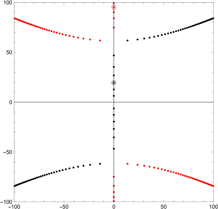
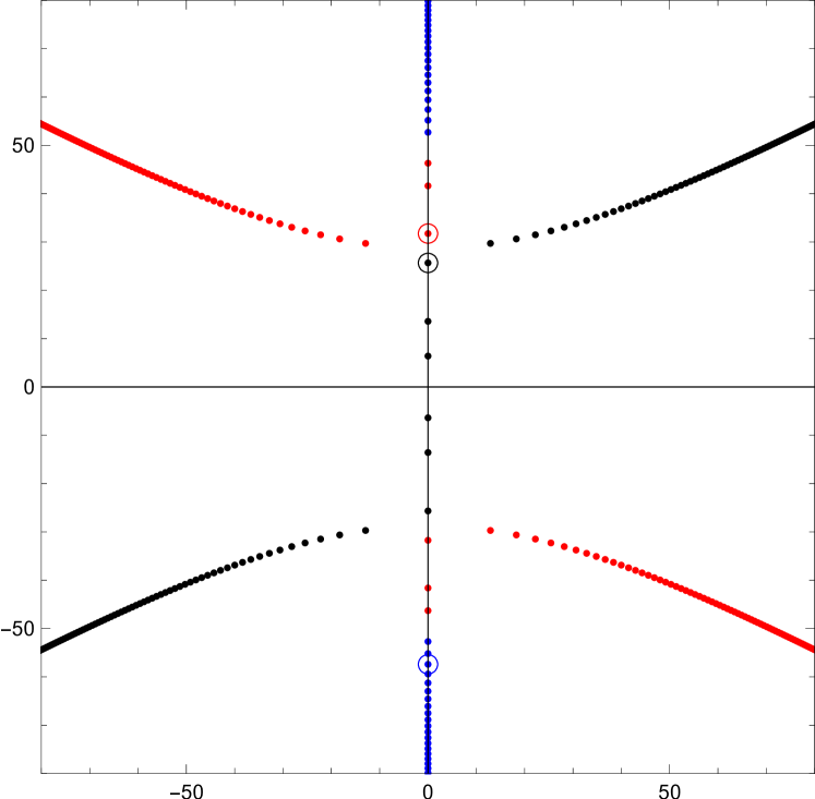
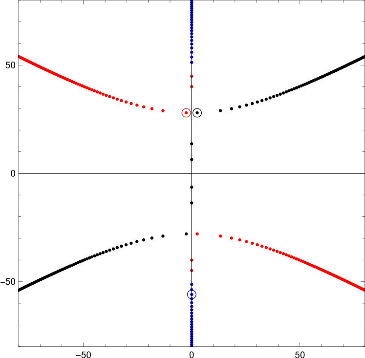
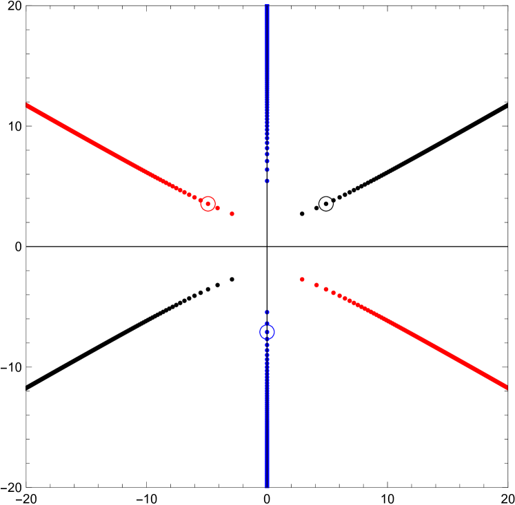
We will now restrict to the case $m=2$ and vary the parameters $r=MR$. The integrand of (6.13) has poles at

$$x-\frac{\alpha\tau_{2}^{3}}{8\pi^{3}}x^{3}=2n\pi i\;,$$ (6.20)

where $n\in\mathbb{Z}$ for the R sector ($\lambda=-1$) and $n\in\mathbb{Z}+\frac{1}{2}$ for the NS sector ($\lambda=1$). The roots of equation (6.20) are

$\displaystyle x_{1}(n)$ $\displaystyle=2n\pi i\,{F\!}\left(\tfrac{1}{3},\tfrac{2}{3};\tfrac{3}{2};-n^{2}\gamma\right)$ (6.21)
$\displaystyle=2n\pi i\left(\tfrac{3}{2}{F\!}\left(\tfrac{1}{3},\tfrac{2}{3};\tfrac{1}{2};1{+}n^{2}\gamma\right){-}\tfrac{\sqrt{3}}{2}\sqrt{1{+}n^{2}\gamma}{F\!}\left(\tfrac{5}{6},\tfrac{7}{6};\tfrac{3}{2};1{+}n^{2}\gamma\right)\right)\;,$
$\displaystyle x_{2}(n)$ $\displaystyle=-2n\pi i\left(\tfrac{1}{2}{F\!}\left(\tfrac{1}{3},\tfrac{2}{3};\tfrac{3}{2};-n^{2}\gamma\right)-\tfrac{1}{2n}\sqrt{-\tfrac{27}{\gamma}}{F\!}\left(-\tfrac{1}{6},\tfrac{1}{6};\tfrac{1}{2};-n^{2}\gamma\right)\right)$ (6.22)
$\displaystyle=-6n\pi i\,{F\!}\left(\tfrac{1}{3},\tfrac{2}{3};\tfrac{1}{2};1+n^{2}\gamma\right)\;,$
$\displaystyle x_{3}(n)$ $\displaystyle=-2n\pi i\left(\tfrac{1}{2}{F\!}\left(\tfrac{1}{3},\tfrac{2}{3};\tfrac{3}{2};-n^{2}\gamma\right)+\tfrac{1}{2n}\sqrt{-\tfrac{27}{\gamma}}\,{F\!}\left(-\tfrac{1}{6},\tfrac{1}{6};\tfrac{1}{2};-n^{2}\gamma\right)\right)$ (6.23)
$\displaystyle=2n\pi i\left(\tfrac{3}{2}{F\!}\left(\tfrac{1}{3},\tfrac{2}{3};\tfrac{1}{2};1{+}n^{2}\gamma\right){+}\tfrac{\sqrt{3}}{2}\sqrt{1{+}n^{2}\gamma}\,{F\!}\left(\tfrac{5}{6},\tfrac{7}{6};\tfrac{3}{2};1{+}n^{2}\gamma\right)\right)\;,$

where

$${F\!}\,(a,b;c;z)\equiv{}_{2}F_{1}(a,b;c;z)\;,\;\;\hbox{ and }\;\;\gamma=\frac{27\alpha\tau_{2}^{3}}{8\pi}\;.$$ (6.24)

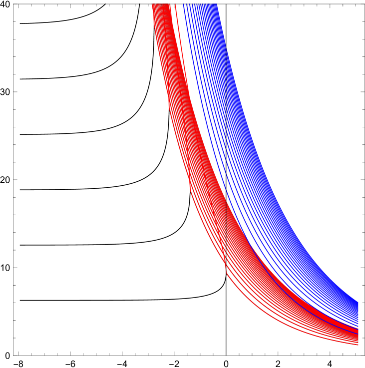
It is helpful to plot these roots in the complex plane for various values of $\gamma$, as in figure 3.

Refer to caption
(a) $\gamma=-0.00001$
Refer to caption
(b) $\gamma=-0.0204785$
Refer to caption
(c) $\gamma=-0.0930842$
Refer to caption
(d) $\gamma=-0.0986693$
Refer to caption
(e) $\gamma=-0.167552$
Refer to caption
(f)   
Figure 3: Figures (a)–(e) are plots of the roots $x_{i}(n)$ for various real values of $\gamma$ and $n\in\mathbb{Z}$. The black points are $x_{1}(n)$, the red are $x_{2}(n)$ and the blue, $x_{3}(n)$. In each plot, the circled points correspond to $n=3$. Note that the plots are not all scaled the same. Figure (f) is a plot of the imaginary parts of the eigenvalues in the upper half plane, plotted against $\log(\gamma)$, for $n\leq 20$.

We divide (6.10) by 2 since we are just interested in right movers and start with $M=0$. We can continue $M$ in the complex plane so that it encircles the poles $x_{i}$ and then return $M$ to zero. When the integration contour is then returned to the positive real axis we pick up contributions from the poles which add $\pm ix_{i}$ to the integral, the $\pm$ depends on which way we encircle the poles.

The one-particle energies we found in section 4 are given by $ix_{1}(n)$ for $n>0$. Since $x_{1}+x_{2}+x_{3}$, we could get the same answer by instead using $-ix_{2}(n)-ix_{3}(n)$.

The hypergeometric function is real if its argument is real and less than or equal to 1. Hence all the $ix_{i}$ are real if $0>\alpha>-\frac{32\pi}{27(2n+1)^{2}}$, but for $\alpha<-\frac{32\pi}{27(2n+1)^{2}}$ then $ix_{3}$ is real and $ix_{1}$ and $ix_{2}$ are a complex conjugate pair.

Finally we note that the roots in the upper half plane are $x_{1}(n)$, $x_{2}(n)$ and $-x_{3}(n)$ for $n>0$.

6.4 Conjectured exact result

We consider the simplest case where the GGE only has a non-zero chemical potential for the charge $I_{3}$. In this case our conjecture is that the modular transform of the expectation value ${\langle\,\exp(\alpha I_{3})\,\rangle}$ is given by the product over terms corresponding to all of the poles $x_{i}$ (6.216.23) in the upper half plane where $\gamma$ has now become

$$\gamma=-\frac{27\alpha\tau^{3}}{8\pi i}\;.$$ (6.25)

(Taking the pole in the upper half plane means that the energies $ix_{1}$ have negative real part and the resulting expressions are convergent).

This conjecture replaces the asymptotic formulae (4.56), (4.58) and (4.60) by

$\displaystyle{\mathrm{Tr}}_{{\text{NS}},+}\left({\hat{q}}^{L_{0}-c/24}e^{\alpha I_{3}}\right)$ $\displaystyle=\hat{\chi}^{{\text{NS}},+}(\tau,\alpha)$
$\displaystyle=q^{h_{0}^{{\text{NS}}}(\tau,\alpha)}\prod_{k=1/2}\left(1+e^{\tau x_{1}(k)}\right)\left(1+e^{\tau x_{2}(k)}\right)\left(1+e^{-\tau x_{3}(k)}\right)\;,$ (6.26)
$\displaystyle{\mathrm{Tr}}_{{\text{R}},+}\left({\hat{q}}^{L_{0}-c/24}e^{\alpha I_{3}}\right)$ $\displaystyle=2^{1/2}\cdot\hat{\chi}^{{\text{NS}},-}(\tau,\alpha)$
$\displaystyle=2^{1/2}\cdot q^{h_{0}^{{\text{NS}}}(\tau,\alpha)}\prod_{k=1/2}\left(1-e^{\tau x_{1}(k)}\right)\left(1-e^{\tau x_{2}(k)}\right)\left(1-e^{-\tau x_{3}(k)}\right)\;,$ (6.27)
$\displaystyle{\mathrm{Tr}}_{{\text{NS}},-}\left({\hat{q}}^{L_{0}-c/24}e^{\alpha I_{3}}\right)$ $\displaystyle=2^{-1/2}\cdot\hat{\chi}^{{\text{R}},+}(\tau,\alpha)$
$\displaystyle=2^{-1/2}\cdot 2\left(1+e^{\tau x_{2}(0)}\right)\,q^{h_{0}^{{\text{R}}}(\tau,\alpha)}\prod_{k=1}\left(1+e^{\tau x_{1}(k)}\right)\left(1+e^{\tau x_{2}(k)}\right)\left(1+e^{-\tau x_{3}(k)}\right)\;,$ (6.28)

where the ground state energies $h_{0}^{{\text{NS}}/{\text{R}}}$ are defined in (4.63) and the roots $x_{i}(k)$ in (6.216.23). Note that $-x_{3}(k)=x_{1}(k)+x_{2}(k)=x_{2}(-k)$, so there are three different ways to write the expressions (6.266.28). Also, since $x_{1}(0)=0$ we have $(1+x^{\tau x_{1}(0)})=2$ and also $x_{2}(0)=-x_{3}(0)$, which is why we only include this term once in (6.28).

As can easily be seen, these have the form of a trace over a space with three sets of fermionic modes, rather than the expected one set.

The asymptotic formulae previously found are recovered by dropping the factors involving the roots $x_{2}$ and $x_{3}$. We note again that the expressions (6.26) etc have identical asymptotic expansions to the previous expressions (4.56) etc.

This gives predictions for the “expectation values” (with the fermionic character divided off)

$\displaystyle{\langle\,e^{\alpha I_{3}}\,\rangle}^{{\text{NS}},+}(-1/\tau)$ $\displaystyle=\frac{\hat{\chi}^{{\text{NS}},+}(\tau,\alpha)}{\chi^{{\text{NS}},+}(\tau)}$
$\displaystyle=q^{h_{0}^{{\text{NS}}}(\tau,\alpha)+1/48}\prod_{k=1/2}\frac{\left(1+e^{\tau x_{1}(k)}\right)\left(1+e^{\tau x_{2}(k)}\right)\left(1+e^{-\tau x_{3}(k)}\right)}{1+q^{k}}\;,$ (6.29)
$\displaystyle{\langle\,e^{\alpha I_{3}}\,\rangle}^{{\text{R}},+}(-1/\tau)$ $\displaystyle=\frac{\hat{\chi}^{{\text{NS}},-}(\tau,\alpha)}{\chi^{{\text{NS}},-}(\tau)}$
$\displaystyle=q^{h_{0}^{{\text{NS}}}(\tau,\alpha)+1/48}\prod_{k=1/2}\frac{\left(1-e^{\tau x_{1}(k)}\right)\left(1-e^{\tau x_{2}(k)}\right)\left(1-e^{-\tau x_{3}(k)}\right)}{1-q^{k}}\;,$ (6.30)
$\displaystyle{\langle\,e^{\alpha I_{3}}\,\rangle}^{{\text{NS}},-}(-1/\tau)$ $\displaystyle=\frac{\hat{\chi}^{{\text{R}},+}(\tau,\alpha)}{\chi^{{\text{R}},+}(\tau)}$
$\displaystyle=q^{h_{0}^{{\text{R}}}(\tau,\alpha)-1/24}\left(1+e^{\tau x_{2}(0)}\right)\prod_{k=1}\frac{\left(1+e^{\tau x_{1}(k)}\right)\left(1+e^{\tau x_{2}(k)}\right)\left(1+e^{-\tau x_{3}(k)}\right)}{1+q^{k}}\;.$ (6.31)

We will now consider the leading order behavoiur of the $x_{i}(n)$ for large negative $\gamma$ and positive $n$. For negative $n$ we can use the relations $x_{1}(-n)=-x_{1}(n)$ and $x_{2}(-n)=-x_{3}(n)$. For large positive $z$ the hypergeometric functions have the following leading order terms

$\displaystyle{}_{2}F_{1}\left(\frac{1}{3},\frac{2}{3};\frac{3}{2};z\right)$ $\displaystyle=$ $\displaystyle\frac{3}{4^{\frac{1}{3}}}e^{-\frac{\pi i}{3}}z^{-\frac{1}{3}}+O(z^{-\frac{2}{3}})\;,$ (6.32)
$\displaystyle\frac{1}{\sqrt{z}}{}_{2}F_{1}\left(-\frac{1}{6},\frac{1}{6};\frac{1}{2};z\right)$ $\displaystyle=$ $\displaystyle\frac{1}{4^{\frac{1}{3}}}e^{\frac{\pi i}{6}}z^{-\frac{1}{3}}+O(z^{-\frac{2}{3}})\;.$ (6.33)

Using these we can find the leading order terms in the $x_{i}$

$\displaystyle x_{1}(n)$ $\displaystyle=$ $\displaystyle 3(2n)^{\frac{1}{3}}\pi e^{\frac{\pi i}{6}}(-\gamma)^{-\frac{1}{3}}+O(\gamma^{-\frac{2}{3}})\;,$ (6.34)
$\displaystyle x_{2}(n)$ $\displaystyle=$ $\displaystyle 3(2n)^{\frac{1}{3}}\pi e^{\frac{5\pi i}{6}}(-\gamma)^{-\frac{1}{3}}+O(\gamma^{-\frac{2}{3}})\;,$ (6.35)
$\displaystyle x_{3}(n)$ $\displaystyle=$ $\displaystyle 3(2n)^{\frac{1}{3}}\pi e^{-\frac{\pi i}{2}}(-\gamma)^{-\frac{1}{3}}+O(\gamma^{-\frac{2}{3}})\;.$ (6.36)

Note that these leading order terms match the pattern of the roots in figure 3 where as $|\gamma|$ increases the roots $x_{1}(n)$ converge towards the rays $e^{\frac{\pi i}{6}}$ and $e^{-\frac{5\pi i}{6}}$, $x_{2}(n)$ towards $e^{\frac{5\pi i}{6}}$ and $e^{-\frac{\pi i}{6}}$ and $x_{3}(n)$ towards $e^{\frac{\pi i}{2}}$ and $e^{-\frac{\pi i}{2}}$.

We can use (6.346.35) to show that for large negative $\alpha$ (equivalently large $\gamma$) the exact expressions and the conjectures match to leading order. If we take the logarithm of (6.266.28) then for large negative $\alpha$ we have

$\displaystyle\log\left(\text{Tr}_{NS,\pm}\left(\hat{q}^{L_{0}-c/24}e^{\alpha I_{3}}\right)\right)=\frac{7\alpha}{1920}+\dots\;,$ (6.37)
$\displaystyle\log\left(\text{Tr}_{R,+}\left(\hat{q}^{L_{0}-c/24}e^{\alpha I_{3}}\right)\right)=-\frac{\alpha}{240}+\dots\;,$ (6.38)

where the $\dots$ represent terms that are suppressed for large negative $\alpha$. For the right hand side we can see that the ground state energies $h_{0}^{\text{NS/R}}$ both vanish as $\alpha$ becomes large and negative. Just looking at the logarithm of the product terms we can rewrite them as a sum

$\displaystyle\log\left(\prod_{k>0}\left(1\pm e^{\tau x_{1}(k)}\right)\left(1\pm e^{\tau x_{2}(k)}\right)\left(1\pm e^{-\tau x_{3}(k)}\right)\right)=$
$\displaystyle\sum_{k>0}\left(\log\left(1\pm e^{\tau x_{1}(k)}\right)+\log\left(1\pm e^{\tau x_{2}(k)}\right)+\log\left(1\pm e^{-\tau x_{3}(k)}\right)\right)\;,$ (6.39)

and if we look at each of the $x_{i}$ contributions separately and replace $x_{i}$ with it’s leading $\alpha$ term then we have sums of the form

$$\sum_{k>0}\log\left(1\pm\exp\left((2\pi)^{\frac{4}{3}}(-i)^{\frac{1}{3}}e^{i\theta_{i}}\left(\frac{k}{-\alpha}\right)^{\frac{1}{3}}\right)\right)\;,$$ (6.40)

where $\theta_{1}=\frac{\pi}{6}$, $\theta_{2}=\frac{5\pi}{6}$ and $\theta_{3}=\frac{\pi}{2}$. If we define the variable $x_{k}=\frac{k}{-\alpha}$ then all $x_{k}$ are positive and we have the spacing $\Delta x=x_{k+1}-x_{k}=\frac{-1}{\alpha}$. We will rewrite (6.40) in terms of the $x_{k}$ to get

$$-\alpha\sum_{k>0}\Delta x\log\left(1\pm\exp\left((2\pi)^{\frac{4}{3}}(-i)^{\frac{1}{3}}e^{i\theta_{i}}x_{k}^{\frac{1}{3}}\right)\right)\;.$$ (6.41)

In the large $\alpha$ limit the sum (6.41) becomes the integral

$$-\alpha\int_{0}^{\infty}dx\log\left(1\pm\exp\left((2\pi)^{\frac{4}{3}}(-i)^{\frac{1}{3}}e^{i\theta_{i}}x^{\frac{1}{3}}\right)\right)\;.$$ (6.42)

We use the substitution $u=-(2\pi)^{\frac{4}{3}}(-i)^{\frac{1}{3}}e^{i\theta_{i}}x^{\frac{1}{3}}$ where we choose the branch of $(-i)^{\frac{1}{3}}$ so that the real part of $u$ tends to positive infinity as $x$ goes to positive infinity. The integrand only has singularities on the imaginary axis in the $u$ plane and hence we can move the integration contour onto the positive real axis without picking up any poles (the additional arc contour that connects the two lines vanishes exponentially as we take the lines to infinity). If we do integration by parts on the integral we then arrive at

$$\frac{3i\alpha e^{-3i\theta_{i}}}{(2\pi)^{4}}\int_{0}^{\infty}du\;u^{2}\log(1\pm e^{-u})=\pm\frac{i\alpha e^{-3i\theta}}{(2\pi)^{4}}\int_{0}^{\infty}du\frac{u^{3}}{e^{u}\pm 1}=\begin{cases}-\frac{i\alpha}{240}e^{-3i\theta_{i}}&-\\ \frac{7i\alpha}{1920}e^{-3i\theta_{i}}&+\end{cases}\;.$$ (6.43)

We can sum over the $i$ to find

$$i\sum_{i=1}^{3}e^{-3i\theta_{i}}=1\;,$$ (6.44)

and finally this gives us the leading large $\alpha$ term for the conjecture

$\displaystyle\log\left(\hat{\chi}^{\text{NS/R},+}\right)=\frac{7\alpha}{1920}+\dots\;,$ (6.45)
$\displaystyle\log\left(\hat{\chi}^{\text{NS},-}\right)=-\frac{\alpha}{240}+\dots\;,$ (6.46)

where the $\dots$ are suppressed terms. These leading terms match those in (6.37) and (6.38) and this provides some non-trivial analytic support for our conjecture.

7 Numerical evidence

Our evidence for the correctness of the formulae (6.26), (6.27) and (6.28) is based mainly on the numerical agreement (to within numerical accuracy) across a range of $\tau$ and $\alpha$. In table 1 we give the values of the modular transforms of our exact results for the expectation values ${\langle\,e^{\alpha I_{3}}\,\rangle}^{{\text{NS}}/{\text{R}}\pm}(-1/\tau)$, the conjectured exact expressions (6.29)–(6.31), and the asymptotic expressions from (4.56)–(4.60) (which we denote $\hat{\chi}_{{\text{NS}}/{\text{R}}\pm}^{(1)}(\tau,\alpha)/\chi_{{\text{NS}}/{\text{R}}\pm}(\tau)$ since it is given by the same form as the conjectured exact expression by only including the roots $x_{1}(k)$).

$\alpha$ $\tau=i$
-0.01 0.9999909023 0.9999909023 0.9999909023 0.9999909023
 $\;-\,5.1697517\times 10^{-126}i$
-0.1 0.9990978822 0.9990978822 0.9990978822 0.9990978822
$\;+\,1.0567308\times 10^{-13}i$
-1 0.9914336696 0.9914091375 0.9914336280 0.9914336696
 $\;-\,0.000044605\,i$
-10 0.9356250621 0.9374288339 0.9326249941 0.9356250621
$\;+\,0.0240515109\,i$
${\langle\,e^{\alpha I_{3}}\,\rangle}^{NS+}(-1/\tau)$ ${\hat{\chi}^{(1)}_{{\text{NS}}+}}/{\chi_{{\text{NS}}+}}(\tau)$ ${\hat{\chi}^{(1,2)}_{{\text{NS}}+}}/{\chi_{{\text{NS}}+}}(\tau)$ ${\hat{\chi}_{{\text{NS}}+}}/{\chi_{{\text{NS}}+}}(\tau)$
$\alpha$ $\tau=(-1+4i)/3$
-0.1 1.0008014459 1.0008014459 1.0008014459 1.0008014459
$\;+\,0.0012333495\,i$ $\;+\,0.0012333495\,i$ $\;+\,0.0012333495\,i$ $\;+\,0.0012333495\,i$
-1 1.0076484482 1.0076114564 1.0076484114 1.0076484482
$\;+\,0.009370977\,i$ $\;+\,0.009397878\,i$ $\;+\,0.009370902\,i$ $\;+\,0.009370977\,i$
-10 1.03116010611 1.01844820142 1.02869050956 1.03116010611
$\;+\,0.0490164216\,i$ $\;+\,0.0639418298\,i$ $\;+\,0.0482967963\,i$ $\;+\,0.0490164216\,i$
${\langle\,e^{\alpha I_{3}}\,\rangle}^{NS-}(-1/\tau)$ ${\hat{\chi}^{(1)}_{{\text{R}}+}}/{\chi_{{\text{R}}+}}(\tau)$ ${\hat{\chi}^{(1,2)}_{{\text{R}}+}}/{\chi_{{\text{R}}+}}(\tau)$ ${\hat{\chi}_{{\text{R}}+}}/{\chi_{{\text{R}}+}}(\tau)$
Table 1: Table of values of a GGE including a coupling to a single charge $I_{3}$ in two different sectors calculated using the exact result from the expression of the charge as a fermion bilinear in one channel and the asymptotic expression, an improved asymptotic expression and a conjectured exact answer in the opposite channel

We also include a modified guess (which we denote $\hat{\chi}_{{\text{NS}}/{\text{R}}\pm}^{(1,2)}(\tau,\alpha)/\chi_{{\text{NS}}/{\text{R}}\pm}(\tau)$) including the product over only the roots $x_{1}(k)$ and $x_{2}(k)$ which is the minimal change required to make the expressions real and single-valued for real $\alpha$ and purely imaginary $\tau$.

For large negative values of $\alpha$, the roots appear to become dense, requiring a very large number of terms to be included in the products (greater than 1000) to achieve reliable numerical results.

8 Conclusions

We have considered the torus partition function for the free fermion model coupled to KdV charges, or equivalently the partition function of generalised Gibbs ensembles. Using the asymptotic expansion of the generalised Gibbs ensemble about $\alpha=0$ allowed us to find an asymptotic expression for the modular transform of the GGE. However the first step involved expanding the GGE as an asymptotic series with vanishing radius of convergence so it is not clear how the above method could be adapted to find the exact from of the modular transformed GGE. The asymptotic expressions take the form of a trace over a fermion Fock space, but if any of the chemical potentials of the higher charges are non-zero then the expression must be wrong. This is most easily seen by looking at a rectangular torus and noting that the original GGE is real but the asymptotic form in the crossed channel is not.

We also analysed the problem from the TBA point of view (in the particular case of coupling to the single charge $I_{3}$ and for the modular transform $S:\tau\to-1/\tau$), to see if the spectrum predicted by TBA was the same as that found from our asymptotic analysis. Our TBA analysis confirmed the energies of the modes we found in the asymptotic analysis but revealed two extra sets of poles which could contribute to the spectrum. One set of these poles solves the reality problem of the asymptotic expression but still gives an expression which is not correct. Including both extra sets, however, gives an expression which agrees numerically with the exact result (in the opposite channel) to a high degree of precision and which we conjecture is the exact result.

The conjectured result for the modular transform of a GGE takes the form of a trace over three copies of the free-fermion Fock space. The interpretation of this result is not clear to us. This could be an artifact, the “extra” copies really being a change to the ground state energy; it could instead indicate that there is a fundamental change to the nature of the Hilbert space in the crossed channel caused by the introduction of a coupling to the charge $I_{3}$.

We have also, so far, only found a conjectured closed form expression for the action of $S$; it remains to prove the conjecture (it could be wrong despite passing numerical and analytic tests) and to extend it to arbitrary elements of the modular group.

This is reminiscent of the spectrum of other perturbed systems which exhibit a similar instability such as the spectrum of the boundary Yee-Lang model perturbed by a large boundary magnetic field [26] (where one copy of a Virasoro representation splits into three copies, one real set and two with complex conjugate energies) and the spectrum of the non-Hermitian spin chain [27]. This has sometimes been interpreted as the result of a phase-transition caused by the instability of the vacuum to the perturbation, something which might also be occurring here. This clearly deserves more study and a better understanding.

In this paper we have only investigated in detail the GGE with one coupling to a single charge. This needs to be extended to several charges and to an infinite set of charges.

It will also be worth investigating the large $\alpha$ limit in which the roots appear to condense onto cuts in the complex plane.

Finally, it is worth looking at other models (such as the Lee-Yang model) for which, at present, there is no closed form for the GGE in either channel to see if any evidence for similar behaviour can be found.

Acknowledgments

We would like to thank B. Doyon, A. Dymarsky, S. Murthy, S. Ross, and G. Takács for helpful discussions at various times. We would also like to thank the JHEP referee for careful reading of the manuscript.

MD would like to thank EPSRC for support under grant EP/V520019/1.

Appendix A Appendix: The free fermion and the Ising model

Firstly, we define the operator $(-1)^{F}$ which squares to 1 and which anticommutes with all fermion modes,

$$\{\psi_{m},(-1)^{F}\}=\{\bar{\psi}_{m},(-1)^{F}\}=0\;.$$ (A.1)

States with eigenvalue $+1$ are called bosonic and those with eigenstate $-1$ are fermionic.

The spaces ${\mathcal{H}}_{\text{NS}}$ and ${\mathcal{H}}_{\text{R}}$ are defined as follows.

A.1 The NS sector

We define the NS vacuum ${{|0\rangle}}_{\text{NS}}$ by

$$\psi_{m}{{|0\rangle}}_{\text{NS}}=0\;,\;\;m>0\;,\;\;\;\;(-1)^{F}{{|0\rangle}}_{\text{NS}}={{|0\rangle}}_{\text{NS}}\;,$$ (A.2)

and the space ${\mathcal{H}}_{\text{NS}}$ has basis

$$\{\psi_{-m_{1}}\ldots\psi_{-m_{n}}{{|0\rangle}}_{\text{NS}}\;,\;\;m_{1}>m_{2}\ldots>m_{n}\geq\tfrac{1}{2}\}\;.$$ (A.3)

In the NS sector, $L_{0}$ takes the form

$$L_{0}=\sum_{m>0}m\,\psi_{-m}\psi_{m}\;.$$ (A.4)

The space ${\mathcal{H}_{\text{NS}}}$ splits into two irreducible representations of the Virasoro algebra with $h=0$ and $h=1/2$ given by the states which have an even or an odd number of fermion modes, respectively. If we define the traces

$\displaystyle{\mathrm{Tr}}_{{\text{NS}},+}(X)={\mathrm{Tr}}_{{\mathcal{H}}_{\text{NS}}}(X)\;,\;\;\;\;\;\;{\mathrm{Tr}}_{{\text{NS}},-}(X)={\mathrm{Tr}}_{{\mathcal{H}}_{\text{NS}}}(\,(-1)^{F}\,X)\;,\;\;$ (A.5)

then we can define

$\displaystyle\chi^{{\text{NS}},+}$ $\displaystyle={\mathrm{Tr}}_{{\text{NS}},+}(q^{L_{0}-c/24})=q^{-1/48}\prod_{n=0}^{\infty}(1+q^{n+1/2})\;,\;\;$ (A.6)
$\displaystyle\chi^{{\text{NS}},-}$ $\displaystyle={\mathrm{Tr}}_{{\text{NS}},-}(q^{L_{0}-c/24})=q^{-1/48}\prod_{n=0}^{\infty}(1-q^{n+1/2})\;.$ (A.7)

These are related to the characters of the irreducible Virasoro representations by

$\displaystyle\chi_{0}$ $\displaystyle={\mathrm{Tr}}_{{\text{NS}}}(\,\tfrac{(1+(-1)^{F})}{2}q^{L_{0}-c/24})\;,\;\;$ $\displaystyle\chi^{{\text{NS}},+}$ $\displaystyle=\chi_{0}+\chi_{1/2}\;,\;\;$ (A.8)
$\displaystyle\chi_{1/2}$ $\displaystyle={\mathrm{Tr}}_{{\text{NS}}}(\,\tfrac{(1-(-1)^{F})}{2}q^{L_{0}-c/24})\;,\;\;$ $\displaystyle\chi^{{\text{NS}},-}$ $\displaystyle=\chi_{0}-\chi_{1/2}\;.$ (A.9)

A.2 The R sector

We define the R vacuum ${{|0\rangle}}_{R}$ by

$$\psi_{m}{{|0\rangle}}_{\text{R}}=0\;,\;\;m>0\;,\;\;\;\;(-1)^{F}{{|0\rangle}}_{\text{R}}={{|0\rangle}}_{\text{R}}\;,$$ (A.10)

and the space ${\mathcal{H}_{\text{R}}}$ has basis

$$\{\psi_{-m_{1}}\ldots\psi_{-m_{n}}{{|0\rangle}}_{\text{R}}\;,\;\;m_{1}>m_{2}\ldots>m_{n}\geq 0\}\;.$$ (A.11)

In the R sector, $L_{0}$ takes the form

$$L_{0}=\sum_{m>0}m\,\psi_{-m}\psi_{m}+\tfrac{1}{16}\;.$$ (A.12)

Note that the space of states with $h=1/16$ is two-dimensional and spanned by the bosonic state ${{|0\rangle}}_{\text{R}}$ and the fermionic state $\psi_{0}{{|0\rangle}}_{R}$.

Correspondingly, The space ${\mathcal{H}_{\text{R}}}$ splits into two copies of irreducible representations of the Virasoro algebra with $h=1/16$ formed of the bosonic and the fermionic states respectively. If we define the traces

$\displaystyle{\mathrm{Tr}}_{{\text{R}},+}(X)={\mathrm{Tr}}_{{\mathcal{H}_{\text{R}}}}(X)\;,\;\;\;\;\;\;{\mathrm{Tr}}_{{\text{R}},-}(X)={\mathrm{Tr}}_{{\mathcal{H}_{\text{R}}}}(\,(-1)^{F}\,X)\;,\;\;$ (A.13)

then we can define

$\displaystyle\chi^{{\text{R}},+}$ $\displaystyle={\mathrm{Tr}}_{{\text{R}},+}(q^{L_{0}-c/24})=2\,q^{1/24}\prod_{n=1}^{\infty}(1+q^{n})=q^{1/24}\prod_{n=0}^{\infty}(1+q^{n})\;,\;\;$ (A.14)
$\displaystyle\chi^{{\text{R}},-}$ $\displaystyle={\mathrm{Tr}}_{{\text{R}},-}(q^{L_{0}-c/24})=0\;.$ (A.15)

These are related to the characters of the irreducible Virasoro representations by

$$\chi^{{\text{R}},+}=2\,\chi_{1/16}\;.$$ (A.16)

A.3 Modular properties

The modular properties of the Virasoro characters are well known. The action of $T$ is obvious, $\chi(\tau+1)=e^{2\pi i(h-c/24)}\chi(\tau)$. The action of $S$ is

$$\begin{pmatrix}\chi_{0}(\tilde{q})\\ \chi_{1/2}(\tilde{q})\\ \chi_{1/16}(\tilde{q})\end{pmatrix}=\begin{pmatrix}\tfrac{1}{2}&\phantom{-}\tfrac{1}{2}&\phantom{-}\tfrac{1}{\sqrt{2}}\\ \tfrac{1}{2}&\phantom{-}\tfrac{1}{2}&-\tfrac{1}{\sqrt{2}}\\ \tfrac{1}{\sqrt{2}}&-\tfrac{1}{\sqrt{2}}&\phantom{-}0\end{pmatrix}\begin{pmatrix}\chi_{0}(q)\\ \chi_{1/2}(q)\\ \chi_{1/16}(q)\end{pmatrix}$$ (A.17)

The modular invariant combination

$$Z=|\chi_{0}|^{2}+|\chi_{1/2}|^{2}+|\chi_{1/16}|^{2}\;,$$ (A.18)

is the partition function of the (purely bosonic) Ising model.

The analysis of the modular properties of the free-fermion model is dictated by the periodicities of the fermion around the two cycles of the torus. We label these by the periodicity on the torus as $A$ and $P$ for anti-periodic and periodic. If we calculate the torus correlation functions as a trace over the states on a cylinder, then the $A$ sector is given by a trace over the NS sector and the $P$ sector by a trace over the R sector. We also need to account for the periodicity along the cylinder - and we do this by the insertion of the operator $(-1)^{F}$ for the $P$ sector but no insertion for the $A$ sector.

If we denote the partition function with periodicities $R$ and $S$ by $Z_{R,S}$, then

$$Z_{A,A}=|\chi^{{\text{NS}},+}|^{2}\;,\;\;Z_{A,P}=|\chi^{{\text{NS}},-}|^{2}\;,\;\;Z_{P,A}=\tfrac{1}{2}|\chi^{{\text{R}},+}|^{2}=2|\chi_{1/16}|^{2}\;,\;\;Z_{P,P}=0\;.\;\;$$ (A.19)

The modular transforms under $T$ are

$$\chi^{{\text{NS}},+}(\tilde{q})=\chi^{{\text{NS}},+}(q)\;,\;\;\chi^{{\text{R}},+}(\tilde{q})=\sqrt{2}\chi^{{\text{NS}},-}(q)\;,$$ (A.20)

and the partition function of the Ising model is the modular invariant combination

$$Z=\tfrac{1}{2}(Z_{A,A}+Z_{A,P}+Z_{P,A}+Z_{P,P})\;.$$ (A.21)

Appendix B Appendix: Modular forms

In this appendix we will list the relevant facts about modular forms that appear in this paper. Proofs of the following statements can be found in [14] and most of the notation will be the same.

The full modular group will be denoted by

$$\Gamma_{1}=\text{SL}(2,\mathbb{Z})\;,$$ (B.1)

and the principal congruence subgroup $\Gamma(N)$ is defined to be the subgroup of $\Gamma_{1}$ such that

$$\Gamma(N)=\{\gamma\in\Gamma_{1}|\gamma\equiv\text{Id}_{2}(\text{mod }N)\}\;.$$ (B.2)

Consider a given matrix $\big{(}\begin{smallmatrix}a&b\\ c&d\end{smallmatrix}\big{)}\in\Gamma$, where $\Gamma$ for us is either $\Gamma_{1}$ or $\Gamma(2)$. If a holomorphic function $f(\tau)$, defined in the upper half plane, has the following transformation property

$$f\left(\frac{a\tau+b}{c\tau+d}\right)=(c\tau+d)^{k}f(\tau)\;,$$ (B.3)

then we say that the function is a holomorphic modular form of weight $k$ on $\Gamma$. We will denote the space of modular forms of weight $k$ on $\Gamma$ by $M_{k}(\Gamma)$.

The group $\Gamma_{1}$ is finitely generated by the matrices

$$\begin{pmatrix}1&1\\ 0&1\end{pmatrix}\;,\;\;\;\begin{pmatrix}0&1\\ -1&0\end{pmatrix}\;,$$ (B.4)

hence we only need to check that a function transforms as a modular form under

$$T:\tau\mapsto\tau+1\;\;\;S:\tau\mapsto\frac{-1}{\tau}\;,$$ (B.5)

to verify it is an element of $M_{k}(\Gamma_{1})$. Similarly the subgroup $\Gamma(2)$ is finitely generated by the matrices

$$\begin{pmatrix}1&2\\ 0&1\end{pmatrix}\;,\;\;\;\begin{pmatrix}1&0\\ 2&1\end{pmatrix}\;,\;\;\;-\text{Id}_{2}\;,$$ (B.6)

hence we only need to check that a function transforms as a modular form under

$$\tilde{T}:\tau\mapsto\tau+2\;\;\;\tilde{S}:\tau\mapsto\frac{\tau}{2\tau+1}\;,$$ (B.7)

to verify it is an element of $M_{k}(\Gamma(2))$. An important fact about the spaces $M_{k}(\Gamma)$ is that they are finite dimensional. The space $M_{2k}(\Gamma_{1})$ is generated by the Eisenstein series (see below) and the space $M_{2k}(\Gamma(2))$ is generated by the Jacobi theta functions (see [14] for definitions of the Jacobi theta functions).

The Eisenstein series $E_{2k}(\tau)$ are elements of $M_{2k}(\Gamma_{1})$ for $k=2,3,\dots$ and they are defined by

$$E_{2k}(\tau)=1+\frac{2}{\zeta(1-2k)}\sum_{n=0}^{\infty}\frac{n^{2k-1}q^{n}}{1-q^{n}}\;,\;\;\;q=e^{2\pi i\tau}\;.$$ (B.8)

For $k=1$ the Eisenstein series $E_{2}(\tau)$ is quasi modular which means that under a modular transform we have the transformation property

$$E_{2}\left(\frac{a\tau+b}{c\tau+d}\right)=(c\tau+d)^{2}E_{2}(\tau)-\frac{6i}{\pi}c(c\tau+d)\;.$$ (B.9)

Additionally we want to consider the Eisenstein series with arguments $2\tau$ and $\frac{1}{2}\tau$. By using the fact that $\tilde{T}=T^{2}$ and $\tilde{S}=(TST)^{2}$ we can see that for $k=2,3,\dots$ we have $E_{2k}(2\tau),E_{2k}(\tau),E_{2k}(\frac{1}{2}\tau)\in M_{2k}(\Gamma(2))$.

We also encounter quasi-modular forms. For our purpose we will define the space of quasi-modular forms of weight $k$ and depth $p$, denoted by $\tilde{M}_{k}^{(\leq p)}(\Gamma)$, to be

$$\tilde{M}_{k}^{(\leq p)}(\Gamma)=\bigoplus_{r=0}^{p}M_{k-2r}(\Gamma)\cdot E_{2}^{r}$$ (B.10)

Finally we define the Serre derivative. The Serre derivative acting on a modular form $f(\tau)$ of weight $k$ is defined to be

$$D_{r}f(\tau)=\frac{1}{2\pi i}\frac{d}{d\tau}f(\tau)-\frac{r}{12}E_{2}(\tau)f(\tau)\;.$$ (B.11)

By using the transformation of $\frac{d}{d\tau}$ under a modular transform we can see that $D_{k}f(\tau)$ is a modular form of weight $k+2$.

References