A Census of the Stellar Populations in the Sco-Cen Complex

Abstract

I have used high-precision photometry and astrometry from the early installment of the third data release of Gaia (EDR3) to perform a survey for members of the stellar populations within the Sco-Cen complex, which consist of Upper Sco, UCL/LCC, the V1062 Sco group, Ophiuchus, and Lupus. Among Gaia sources with $\sigma_{\pi}<1$ mas, I have identified 10,509 candidate members of those populations. I have compiled previous measurements of spectral types, Li equivalent widths, and radial velocities for the candidates, which are available for 3169, 1420, and 1740 objects, respectively. In a subset of candidates selected to minimize field star contamination, I estimate that the contamination is $\lesssim 1$% and the completeness is $\sim 90$% at spectral types of $\lesssim$M6–M7 for the populations with low extinction (Upper Sco, V1062 Sco, UCL/LCC). I have used that cleaner sample to characterize the stellar populations in Sco-Cen in terms of their initial mass functions, ages, and space velocities. For instance, all of the populations in Sco-Cen have histograms of spectral types that peak near M4–M5, which indicates that they share similar characteristic masses for their initial mass functions ($\sim 0.15$–0.2 $M_{\odot}$). After accounting for incompleteness, I estimate that the Sco-Cen complex contains nearly 10,000 members with masses above $\sim 0.01$ $M_{\odot}$. Finally, I also present new estimates for the intrinsic colors of young stars and brown dwarfs ($\lesssim 20$ Myr) in bands from Gaia EDR3, the Two Micron All Sky Survey, the Wide-field Infrared Survey Explorer, and the Spitzer Space Telescope.

1. Introduction

Scorpius-Centaurus (Sco-Cen, Preibisch & Mamajek, 2008) is the nearest OB association to the Sun (100–200 pc, de Zeeuw et al., 1999). It contains several thousand stars with ages of 10–20 Myr that historically have been divided into three subgroups: Upper Sco, Upper Centaurus-Lupus (UCL), and Lower Centaurus-Crux (LCC, Blaauw, 1964; de Zeeuw et al., 1999). More recent studies have suggested that UCL and LCC are two sections of a continuous distribution of stars (Rizzuto et al., 2011) and have identified an additional compact group associated with V1062 Sco (Röser et al., 2018; Damiani et al., 2019). The subgroups of Sco-Cen overlap spatially and kinematically with hundreds of younger stars ($\lesssim 6$ Myr) associated with dark clouds in Ophiuchus (Wilking et al., 2008) and Lupus (Comerón, 2008), which together comprise the Sco-Cen complex.

The stellar populations in Sco-Cen are appealing for studies of star and planet formation because they are nearby and contain large samples of stars and circumstellar disks that span a range of ages and evolutionary stages. However, the richest populations in Sco-Cen, Upper Sco and UCL/LCC, are distributed across a large area of sky ($\sim 60\arcdeg\times 20\arcdeg$), so a census of the complex requires wide-field data that can distinguish Sco-Cen members from numerous field stars. Discriminating among the overlapping populations in Sco-Cen poses an additional challenge.

The Gaia mission is performing an all-sky survey to measure precise photometry, proper motions, and parallaxes for more than a billion stars (Perryman et al., 2001; de Bruijne, 2012; Gaia Collaboration et al., 2016). Those data are extremely valuable for identifying candidate members of nearby stellar associations. The first two data releases of Gaia (DR1 and DR2) have been extensively utilized for that purpose in Sco-Cen (Cook et al., 2017; Goldman et al., 2018; Luhman et al., 2018; Manara et al., 2018; Röser et al., 2018; Wilkinson et al., 2018; Cánovas et al., 2019; Damiani et al., 2019; Esplin & Luhman, 2020; Galli et al., 2020; Melton, 2020; Luhman & Esplin, 2020; Luhman, 2020; Teixeira et al., 2020; Kerr et al., 2021). However, because of the complex kinematic structure of Sco-Cen and varying approaches to membership analysis, some of the resulting samples of candidates have differed substantially (e.g., Luhman, 2020).

The early installment of the third data release of Gaia (EDR3) has improved upon DR2 in terms of completeness and astrometric and photometric precisions (Gaia Collaboration et al., 2021). I have taken EDR3 as an opportunity to perform a thorough census of the stellar populations in the Sco-Cen complex. I have used data from EDR3 to characterize the kinematics of the different populations within Sco-Cen and I have identified sources from EDR3 that have kinematics and photometry that support membership in those populations (Section 2). I have compiled previous measurements of spectral types, Li equivalent widths, and radial velocities for those candidates and I have examined the stellar populations in Sco-Cen in terms of their initial mass functions (IMFs), ages, and space velocities (Section 3). A separate study identifies and classifies the circumstellar disks among the candidate members of Sco-Cen (Luhman, 2021).

2. Identification of Candidate Members of Sco-Cen

2.1. Kinematic Selection Criteria

For my survey of Sco-Cen, I have considered the area from $l=283$ to $2\arcdeg$ and $b=-12$ to $35\arcdeg$, which is large enough to extend beyond the outer boundary of the Sco-Cen OB subgroups that was adopted by de Zeeuw et al. (1999).

This study makes use of the following measurements from Gaia EDR3: photometry in bands at 3300–10500 Å ($G$), 3300–6800 Å ($G_{\rm BP}$), and 6300-10500 Å ($G_{\rm RP}$); proper motions and parallaxes ($G\lesssim 20$); radial velocities originating from Gaia DR2 ($G\sim 4$–12); and the renormalized unit weight error (RUWE, Lindegren, 2018). The latter serves as an indicator of the goodness of fit for the astrometry. As done in my previous studies of Sco-Cen populations with Gaia DR2 (Esplin & Luhman, 2020; Luhman & Esplin, 2020; Luhman, 2020), I adopt a threshold of RUWE$<$1.6 when I wish to consider astrometry from EDR3 that is likely to be reliable.

Ideally, the kinematic identification of members of an association would be performed with three-dimensional space velocities. However, most stars in EDR3 lack measurements of radial velocities, which (in conjunction with proper motions and parallactic distances) are needed for calculating space velocities. Therefore, I rely on the proper motions and parallaxes from EDR3 for kinematic selection of candidates in Sco-Cen. Because of projection effects, stars that share the same space velocity but are distributed across a large area of sky can exhibit a broad range of proper motions. To reduce such projection effects, I analyze the Gaia astrometry in terms of a “proper motion offset” ($\Delta\mu_{\alpha,\delta}$), which is defined as the difference between the observed proper motion of a given star and the motion expected at the celestial coordinates and parallactic distance of the star for a characteristic space velocity for the association (e.g., the median velocity), as done in my previous studies of Gaia data for nearby associations (Esplin et al., 2017; Esplin & Luhman, 2019, 2020; Luhman, 2018, 2020; Luhman & Esplin, 2020). The proper motion offsets in this survey are calculated relative to the motions expected for a space velocity of $U,V,W=-5,-16,-7$ km s^-1, which approximates the median velocity of Upper Sco (Luhman & Esplin, 2020, Section 3.5). For parallactic distances, I adopt the geometric values estimated by Bailer-Jones et al. (2021) from EDR3 parallaxes.

To characterize the kinematics of populations in Sco-Cen with Gaia EDR3, I follow the procedures previously applied to data from Gaia DR2 for Upper Sco (Luhman & Esplin, 2020) and Lupus (Luhman, 2020). I begin by identifying candidates for young low-mass stars toward Sco-Cen by selecting sources from Gaia EDR3 that have celestial coordinates within my survey field, parallaxes within a range encompassing Sco-Cen ($\pi=4$–11 mas), small relative errors in parallax ($\pi/\sigma_{\pi}\geq 20$), reliable astrometry (RUWE$<$1.6), colors corresponding to low-mass stars ($G_{\rm BP}-G_{\rm RP}$=1.4–3.4, $\sim$K5–M5, $\sim$0.15–1 $M_{\odot}$), and positions above the single-star sequence for the Tuc-Hor association (45 Myr, Bell et al., 2015) in $M_{G_{\rm RP}}$ versus $G_{\rm BP}-G_{\rm RP}$. The resulting candidates are plotted in diagrams of proper motion offset versus parallactic distance in the top row of Figure 1. Those data exhibit rich overlapping concentrations, which correspond to the groups in Sco-Cen, and a sparse population that is roughly uniform in density at a given distance, which consists of members of the field (young stars and older unresolved binaries). To discriminate between the Sco-Cen members and field stars, I have applied a Gaussian mixture model (GMM) to the proper motion offsets and distances using the mclust package in R (R Core Team, 2013; Scrucca et al., 2016). As done by Luhman & Esplin (2020) in analysis of DR2 data in Sco-Cen, I adopted a model that contains three components for Sco-Cen (V1062 Sco, Upper Sco/Ophiuchus/Lupus, UCL/LCC) and a noise component for the field stars. The stars with $>$90% probability of membership in Sco-Cen according to that model (i.e., the sum of the membership probabilities for the three Sco-Cen components is $>$90%) are adopted as an initial sample of candidate members of Sco-Cen for the following analysis.

The GMM has provided a means of separating candidate members of Sco-Cen from field stars. To isolate the kinematics of the individual populations in Sco-Cen, I can examine the candidates within the areas where the populations are concentrated, which are revealed by my Sco-Cen candidates as well as previous surveys of Sco-Cen. The Upper Sco association is projected against the Ophiuchus clouds and extends well beyond them (de Zeeuw et al., 1999). Esplin et al. (2018) attempted to identify the area within which Ophiuchus members dominate by using Gaia DR2 data to measure the spatial variation of relative ages of stars in the vicinity of Ophiuchus. They defined a boundary that encompassed stars with systematically younger ages, which roughly coincided with the edges of the Ophiuchus clouds. Meanwhile, Luhman & Esplin (2020) defined a triangular field that contains the central concentration of stars in Upper Sco (and Ophiuchus). In Luhman (2020), I found that most of the members of Lupus are within four fields that encompass clouds 1–4 (see also Galli et al., 2020). The members of the V1062 Sco group are clustered within a few degrees of that star (Röser et al., 2018; Damiani et al., 2019; Luhman & Esplin, 2020). Finally, based on the candidates identified with my GMM and similar work with DR2 data in Luhman & Esplin (2020), members of UCL/LCC exhibit the widest spatial distribution among the populations in Sco-Cen, extending across the entire length of the OB subgroups as defined by de Zeeuw et al. (1999).

In each of five panels in Figures 1 and 2, I have plotted the proper motion offsets and parallactic distances of all Sco-Cen candidates identified with the GMM that are located within the following five regions: 1) the Ophiuchus field from Esplin et al. (2018); 2) the triangular field in the center of Upper Sco from Luhman & Esplin (2020), excluding Ophiuchus; 3) fields toward Lupus clouds 1–4 from Luhman (2020); 4) a $2\arcdeg$ radius field toward V1062 Sco; and 5) a field encompassing most of the stars in the UCL/LCC component from the GMM, which I define as $l=295$–$312\arcdeg$/$b=0$–$20\arcdeg$ and $l=312$–$343\arcdeg$/$b=10$–$20\arcdeg$. In these data, the kinematics of the individual populations are readily identified. Each of the diagrams for V1062 Sco and UCL/LCC exhibits a single well-defined cluster. The former is compact and the latter is much broader, particularly in distance, which is consistent with the relative sizes of these populations on the sky. I have used the functions kde2d and bandwidth.nrd from the MASS package in R (Venables & Ripley, 2002) to calculate density maps in $(\pi,\Delta\mu_{\alpha})$ and $(\pi,\Delta\mu_{\delta})$ for V1062 Sco and UCL/LCC and I have marked the resulting contours that encompass most ($>95$%) of the candidates in each cluster. For each of the fields toward Ophiuchus and Upper Sco, the kinematic data show one dominant cluster that corresponds to the targeted population and a smaller number of outliers. For the Ophiuchus field, the data for the outliers are consistent with membership in Upper Sco or UCL/LCC. The outliers in the Upper Sco field are likely members of UCL/LCC. In the kinematic diagram for the Lupus fields, the most compact group contains stars associated with the clouds while the remaining stars are likely members of UCL/LCC (Luhman, 2020). As done for V1062 Sco and UCL/LCC, I have marked density contours in Figures 1 and 2 for the clusters that correspond to members of Ophiuchus, Upper Sco, and Lupus.

I have used the contours in Figures 1 and 2 as criteria for identifying candidate members of the Sco-Cen populations. I have retrieved from EDR3 all sources that have positions within my survey field, parallax errors of $\sigma_{\pi}<1$ mas, and distances and proper motion offsets that overlap at 1 $\sigma$ with any of the five pairs of contours. A criterion involving RUWE is not applied. This sample will be further refined with Gaia photometry in the next section.

I note that the selection of candidates using the contours in Figures 1 and 2 has negligible dependence on the precise value of the velocity assumed when calculating the proper motion offsets. The populations in Sco-Cen span a fairly small range of space velocities (5–10 km s^-1, Section 3.5), so adopting a different velocity within that range (e.g., the median velocity of UCL/LCC instead of the median velocity of Upper Sco) would result in a small shift in the proper motion offsets (and their contours) that is nearly the same for all Sco-Cen members, leaving the selection of candidates unaffected.

2.2. Photometric Selection Criteria

The candidate members of Sco-Cen selected via kinematics in the previous section can be further refined with color-magnitude diagrams (CMDs) consisting of $M_{G_{\rm RP}}$ versus $G_{\rm BP}-G_{\rm RP}$ and $M_{G_{\rm RP}}$ versus $G-G_{\rm RP}$. Since the V1062 Sco group and UCL/LCC are tied as the oldest populations in Sco-Cen (Luhman & Esplin, 2020), any members of Sco-Cen should appear on or above the sequences of those populations in CMDs. The sequence for V1062 Sco is more easily measured since that group is much more compact than UCL/LCC. Selecting candidates within a small area that encompasses the bulk of the V1062 Sco group produces a sample that has little contamination from field stars or other populations in Sco-Cen. In the top row of Figure 3, I have plotted two CMDs for the candidates with kinematics consistent with V1062 Sco and positions within a radius of $2\arcdeg$ from the center of that group. Photometry with errors greater than 0.1 mag has been excluded. As expected, the sequences for V1062 Sco are clearly defined. I have marked boundaries in Figure 3 that follow the lower envelopes of those sequences.

In each of the two CMDs in the bottom row of Figure 3, I have plotted all kinematic candidates in Sco-Cen from the previous section that have photometry with errors less than 0.1 mag in both bands for a given CMD. I have included the boundaries defined with the sequences for V1062 Sco, and I have rejected candidates that appear below either of them unless they exhibit infrared (IR) excess emission in photometry from the Wide-field Infrared Survey Explorer (WISE, Wright et al., 2010). Stars with excesses have been identified using colors within the WISE bands (W1$-$W2, W1$-$W3, W1$-$W4, Luhman, 2021). The latter candidates are retained since stars that are occulted by circumstellar disks can appear in scattered light, which results in unusually faint apparent magnitudes at a given color. When rejecting candidates with the CMD boundaries, the absolute magnitudes of the candidates are calculated for the 1 $\sigma$ upper limit on the distance from Bailer-Jones et al. (2021) (i.e., the brightest $M_{G_{\rm RP}}$ allowed at 1 $\sigma$). If that upper limit is greater than 200 pc, a value of 200 pc is adopted since it approximates the maximum distance for members of Sco-Cen (Figure 1). The number of candidates satisfying at least one CMD and not rejected by either CMD is 10,104. The number of additional candidates that fell below the boundary of a CMD but were retained as viable candidates because of IR excess is 91.

Some kinematic candidates were not plotted in either of the CMDs in Figure 3 because photometry is unavailable or uncertain in one or more Gaia bands. In most cases, this is due to the faintness of a star or its close proximity to a brighter star. The former tend to have large astrometric uncertainties (due to their faint magnitudes) while the latter tend to be brighter and have more precise astrometry. A natural division between these two groups appears near $\sigma_{\pi}\sim 0.4$ mas. Among these candidates that lack photometry for CMDs, I have rejected those with $\sigma_{\pi}>0.4$ mas except for two objects that have IR excess emission, which are retained. I also have rejected candidates with $\sigma_{\pi}<0.4$ mas if they are within $5\arcsec$ from a star that shares a similar proper motion and parallax and that is rejected by the CMDs (i.e., a likely companion to a rejected star). The remaining 312 candidates that lack the data for CMDs and have $\sigma_{\pi}<0.4$ mas are retained.

The 10,509 candidates are presented in Table 1. The spatial distribution of the kinematic populations among these candidates is illustrated in Figure 4. For reference, I have marked in those maps the boundary of Sco-Cen from de Zeeuw et al. (1999) and the fields in Upper Sco, Ophiuchus, Lupus, and V1062 Sco that were mentioned in Section 2.1. Since the kinematics of the populations in Sco-Cen overlap (Figure 1), data for a given candidate can be consistent with multiple populations. Two of the maps in Figure 4 show the candidates with kinematics consistent with Upper Sco, Ophiuchus, or Lupus (top) and the candidates consistent with V1062 Sco (middle). To better trace the spatial distribution for UCL/LCC and minimize contamination from the other populations, the third map shows candidates with kinematics indicative of only UCL/LCC and no other population. The latter map illustrates how UCL/LCC extends across Lupus, Ophiuchus, and Upper Sco. As a result, pre-Gaia surveys for members of the latter regions have been subject to contamination from UCL/LCC (Galli et al., 2020; Luhman & Esplin, 2020; Luhman, 2020).

2.3. Non-kinematic Candidate Companions

I have attempted to identify companions to the candidates in Table 1 that are in Gaia EDR3 but did not satisfy the kinematic criteria that produced those candidates. To do that, I retrieved sources from EDR3 that are located within $5\arcsec$ from the candidates and that satisfy any of these three sets of criteria: 1) a parallax measurement is unavailable or uncertain ($\sigma_{\pi}>1$ mas) and the boundaries in both CMDs in Figure 3 are satisfied for a distance of 200 pc (the most optimistic distance to adopt); 2) the parallax error is below 1 mas, the kinematics do not satisfy any of the criteria from Figures 1 and 2, and both CMDs are satisfied for 200 pc or IR excess emission is present (all of these sources share similar proper motions with their potential companions from Table 1); 3) photometry for CMDs is unavailable, the kinematics do not satisfy any of the criteria from Figures 1 and 2, and the parallax and proper motion are within roughly similar to those of the candidate from Table 1 that it is near ($\Delta\pi<2$ mas, $\Delta\mu_{\alpha,\delta}<5$ mas). The resulting samples contain 48, 100, and 47 sources, respectively. These 195 candidate companions are presented in Table 2. Many of the candidates have large values of RUWE that would suggest unreliable astrometry, which could explain why they did not satisfy the kinematic criteria for membership.

2.4. Compilation of Data for Candidates

In Tables 1 and 2, I have compiled various data that are useful for analyzing the candidate members of Sco-Cen. All candidates were selected from Gaia EDR3, so all have source names from that catalog. To facilitate comparison to previous work, I have included the names for matching sources from Gaia DR2 that are within a separation of $0\farcs 1$ and the designations from a selection of other catalogs. The remaining contents of Tables 1 and 2 consist of the equatorial coordinates, proper motion, parallax, RUWE, and photometric magnitudes from Gaia EDR3; measurements of spectral types and the types adopted in this work; the average of previous measurements of equivalent widths for Li at 6707 Å; distance estimate based on Gaia EDR3 parallax (Bailer-Jones et al., 2021); the most accurate radial velocity measurement from previous studies that has an error less than 4 km s^-1; $UVW$ velocities (Section 3.5; only for Table 1); a flag indicating the populations with which the kinematics are consistent based on the criteria in Figures 1 and 2 (only for Table 1); a flag indicating the regions of Sco-Cen in which a candidate is located; the designations and angular separations of the closest sources within $3\arcsec$ from the Point Source Catalog of the Two Micron All Sky Survey (2MASS, Skrutskie et al., 2006) and the WISE All-Sky Source Catalog (Cutri et al., 2012), the AllWISE Source Catalog, or the AllWISE Reject Catalog (Cutri et al., 2013a); and flags indicating whether the Gaia source is the closest match in EDR3 for the 2MASS and WISE sources. The numbers of candidates in Table 1 that have measurements of spectral types, Li, and radial velocities are 3169, 1420, and 1740, respectively. Three additional objects have been observed spectroscopically, but their classifications are uncertain (i.e., no adopted spectral type in Table 1). For close pairs that were likely unresolved during previous spectroscopy, the spectroscopic data have been assigned to the component that is brighter in $G$ from EDR3. For the closest matching WISE sources, Luhman (2021) provides a catalog of IR photometry from 2MASS and WISE, flags indicating whether those data exhibit excess emission from disks, and classifications of the evolutionary stages of any detected disks.

2.5. Comparison of Gaia, 2MASS, and WISE Limits

Given that 2MASS and WISE are the primary sources of IR photometry for the candidate members of Sco-Cen, it is useful to compare their limits to that of Gaia EDR3. For this comparison, I have chosen the bands from 2MASS and WISE that are most sensitive to late-type members of Sco-Cen, which correspond to $J$ and W1 given the colors of such objects and the relative completeness limits among the 2MASS and WISE bands (Skrutskie et al., 2006; Cutri et al., 2013b; Eisenhardt et al., 2020; Marocco et al., 2021). The completeness limits in $J$ and W1 are $\gtrsim 15.8$ and 17, respectively, for most of the sky. In the CMDs in Figure 3, I have marked the values of $M_{G_{\rm RP}}$ that correspond to those limits assuming the typical colors of young stars (Section 3.2) and a distance just beyond the far side of Sco-Cen (200 pc). Assuming smaller distances would move the limits down in those diagrams. A comparison of the $J$ and W1 limits and the sequences for Sco-Cen indicates the following for members of Sco-Cen: WISE is deeper than 2MASS; 2MASS and WISE are deeper than $G_{\rm BP}$; 2MASS probably has a roughly similar depth as $G$ and $G_{\rm RP}$. All Sco-Cen members with $\sigma_{\pi}<1$ mas (the threshold used for the candidates in Figure 3) should be detected in W1 as long as they are not blended with another star.

2.6. Field Star Contamination

Additional criteria can be applied to the candidate members of Sco-Cen identified in Sections 2.1 and 2.2 (Table 1) to minimize contamination from field stars. The map of the candidates in Figure 4 demonstrates that all of the populations in Sco-Cen are concentrated within the boundaries of the OB subgroups from de Zeeuw et al. (1999). Therefore, considering only candidates within that area reduces the relative contribution of field stars to the sample. Contamination is further reduced by requiring reliable astrometry (RUWE$<$1.6) and $\sigma_{BP}<0.1/\sigma_{RP}<0.1$ or $\sigma_{G}<0.1/\sigma_{RP}<0.1$ so that the candidates have satisfied at least one of the two CMDs in Figure 3.

I have estimated the field star contamination in the subset of candidates from Table 1 that satisfy the preceding criteria. To do that, I shifted the kinematic thresholds from Figures 1 and 2 by +20 mas yr^-1 in $\Delta\mu_{\alpha}$ and +12 mas yr^-1 in $\Delta\mu_{\delta}$, retrieved sources from EDR3 within the Sco-Cen survey field that satisfied those shifted thresholds, and applied the CMD boundaries in Figure 3 to the resulting kinematic candidates. Those steps were repeated for seven additional shifts that surround the thresholds for Sco-Cen: (+20,0), (+20,$-$12), (0,+12), (0,$-$12), ($-$20,+12), ($-$20,0) and ($-$20,$-$12) mas yr^-1. The sizes of the shifts were selected to be large enough that the new thresholds did not overlap with the kinematics of Sco-Cen. In the eight resulting samples of field stars that satisfied the CMD criteria for Sco-Cen, the numbers of stars range from $\sim 40$–100 for $\sigma_{\pi}<0.5$ mas, which is a small variation relative to the thousands of candidates in Sco-Cen. However, the variation in the numbers of stars is greater for $\sigma_{\pi}>0.5$ mas and the highest numbers occurred for the kinematic thresholds that were closest to the proper motion offsets exhibited by the bulk of distant field stars beyond Sco-Cen. A small fraction of those numerous distant stars can have parallax measurements within the range for Sco-Cen due to their large errors, enabling their selection as kinematic candidates for Sco-Cen. When their absolute magnitudes are calculated using the erroneously small parallactic distances, they appear anomalously faint in CMDs. Stars of this kind comprise the large clump below the main sequence in the $G_{\rm BP}/G_{\rm RP}$ CMD for Sco-Cen candidates in Figure 3. In the $G/G_{\rm RP}$ CMD, the clump straddles the bottom of the main sequence. When those stars have photometry in $G_{\rm BP}$ and $G_{\rm RP}$, they are rejected by that CMD. But for the clump stars that only have $G$ and $G_{\rm RP}$, many of them appear above the boundary in that CMD and survive to contaminate the sample of candidates. This source of contamination can be greatly reduced by considering only candidates with $\sigma_{\pi}<0.5$ mas, which corresponds to 10,145 of the 10,509 candidates in Table 1.

In Figure 5, I have plotted histograms of $G_{\rm BP}-G_{\rm RP}$ and $G-G_{\rm RP}$ for Sco-Cen candidates from Table 1 that satisfy the criteria described thus far in this section for minimizing contamination: locations within the Sco-Cen boundary from de Zeeuw et al. (1999), RUWE$<$1.6, $\sigma_{\pi}<0.5$ mas, and $\sigma_{BP}<0.1/\sigma_{RP}<0.1$ or $\sigma_{G}<0.1/\sigma_{RP}<0.1$. The resulting numbers of candidates in the two histograms are 7272 and 8000, respectively. For comparison, I have included in Figure 5 the average histograms for the eight samples of field stars described previously after applying the same criteria for minimizing field stars. The resulting contaminants consist of A/F/G stars on the main sequence and M stars appearing above the main sequence. The former source of contamination is expected given that the CMD boundaries for selecting candidates intersect with the main sequence (Figure 3). The group of M-type field likely consists of both young stars and older unresolved binaries. The field star histograms for $G_{\rm BP}/G_{\rm RP}$ and $G/G_{\rm RP}$ contain $\sim$40 and 70 stars, respectively, which correspond to $\sim$0.6% and 0.9% of the Sco-Cen candidates. Requiring accurate photometry in $G_{\rm BP}$ and $G_{\rm RP}$ produces the cleanest sample of candidates, but the sample that only requires $G$ and $G_{\rm RP}$ reaches later spectral types.

Spectroscopy can be used to assess whether individual candidates are likely to be field stars or members of Sco-Cen. Measurements of radial velocities can further constrain membership by enabling the calculation of $UVW$ velocities, although multiple epochs are necessary to check whether the velocities are affected by orbital motion within binary systems. The Li absorption line at 6707 Å and gravity-sensitive spectral features serve as diagnostics of youth that can distinguish between members of Sco-Cen and older field stars. To illustrate the application of Li for this purpose, I have plotted in Figure 6 the Li equivalent widths compiled in Table 1 versus spectral type for the samples in Ophiuchus, Lupus, Upper Sco, and UCL/LCC defined in Section 3.1. The sample for V1062 Sco has been omitted since few of its candidates have Li data. In low-mass stars, Li is depleted over time at a rate that varies with spectral type (Bildsten et al., 1997). In Figure 6, the candidates that exhibit unusually weak Li relative to other candidates at a given spectral type may be older field stars. It would be useful to better test the membership of those stars with weak Li by searching for evidence of youth with gravity-sensitive features and comparing their $UVW$ velocities to those of other members. In addition, measuring Li for a larger number of M-type candidates in UCL/LCC and the V1062 Sco group would provide constraints on their ages (Stauffer et al., 1999; Mentuch et al., 2008; Yee & Jensen, 2010), which could be compared to the ages inferred from their CMDs (Section 3.4).

2.7. Completeness

In the previous section, I found that field star contamination among the candidate members of Sco-Cen is reduced by considering only candidates that have RUWE$<$1.6, $\sigma_{\pi}<0.5$ mas, and $\sigma_{BP}<0.1/\sigma_{RP}<0.1$ or $\sigma_{G}<0.1/\sigma_{RP}<0.1$. These criteria will be adopted when characterizing the stellar populations in Sco-Cen in Section 3. Therefore, it is useful to estimate the completeness of the samples of candidates defined in that way.

Gaia EDR3 has a high level of completeness at $G\lesssim 19$–20 except for very crowded regions and the brightest stars that experience saturation (Fabricius et al., 2021). $G$-band measurements are available for $>99$% of the sources in EDR3 (Gaia Collaboration et al., 2021). For sources with data in $G$ that are within the boundary of Sco-Cen from de Zeeuw et al. (1999), I have plotted the fraction that satisfy the previously listed criteria for reducing field star contamination versus $G$ in Figure 7. The fraction is $\sim 85$% at $G<12$ and $\sim 90$–95% at $G=12$–19.5. The lower values at brighter magnitudes are due to the restriction on RUWE. These data indicate that the cleanest samples of candidate members of Sco-Cen may be missing $\sim 10$% of the members. Note that some of those missing members are likely among the candidates in Table 1 (and Table 2), but they are in regimes of RUWE, $\sigma_{\pi}$, and photometric errors in which field star contamination is higher.

2.8. Comparison to Previous Surveys

Table 3 lists many of the studies from the last two decades that have identified candidate members of populations in Sco-Cen or have studied samples of candidates from other sources. Most surveys of Lupus have been omitted since they were scrutinized with Gaia DR2 by Luhman (2020) and the results have not changed qualitatively with EDR3. For each study in Table 3, I have compiled the number of candidate members in its sample, the number of those candidates that have parallax measurements with $\sigma_{\pi}<1$ mas from EDR3, and the number of the candidates with parallaxes that have been classified in this work as candidate members of any Sco-Cen population (i.e., they appear in Table 1).

Because of saturation, Gaia EDR3 is increasingly incomplete at decreasing magnitudes below $G\sim 4$ (Gaia Collaboration et al., 2016; Fabricius et al., 2021). As a result, many of the brightest stars that have been previously proposed as members of Sco-Cen (e.g., Antares) are absent from my catalog of candidates. For instance, 14 of the candidates from de Zeeuw et al. (1999) lack parallax measurements from EDR3 and have Hipparcos magnitudes of $\lesssim 4$ (van Leeuwen, 2007). The analysis of the main sequence turn-off in Sco-Cen by Pecaut & Mamajek (2016) included seven additional stars of that kind. All of those 21 stars have parallax and proper motion measurements from Hipparcos. Those data satisfy the kinematic criteria for membership from Section 2.1 for 11 of the 21 stars, although most of the parallaxes have large errors by the standards of Gaia ($\sigma_{\pi}>0.5$ mas). In addition, three of those 10 stars have astrometry from Gaia DR2 that is inconsistent with membership.

The membership classifications in this work suggest that most previous samples of candidate members of Sco-Cen have had substantial contamination from field stars, which often was expected (de Zeeuw et al., 1999). Even among the recent studies that utilize data from Gaia, there are significant differences in distinguishing between field stars and members of Sco-Cen and between members of the multiple populations in Sco-Cen, which is a reflection of the variety of analysis methods and the overlapping spatial locations and kinematics of those populations (Galli et al., 2020; Luhman, 2020). To illustrate some of those differences in membership classifications, I discuss two of the latest surveys in Sco-Cen that have used data from Gaia EDR3, Squicciarini et al. (2021) and Grasser et al. (2021).

Squicciarini et al. (2021) selected candidate members of Upper Sco from Gaia EDR3 by applying criteria that encompassed a concentration of stars within a space defined by equatorial coordinates, parallax, and tangential velocities. Thresholds on $\sigma_{\pi}/\pi$ and $G$ were also employed. Squicciarini et al. (2021) did not include criteria for selecting stars based on evidence of youth, such as positions in CMDs (Section 2.2). When applying their selection criteria, I arrive at a sample that is slightly larger than the size quoted in Squicciarini et al. (2021) (2862 versus 2745). They did not present a tabulation of their candidates, so the source of this difference is unclear. In my version of their sample, $\sim$69% of the candidates satisfy my criteria for membership in Upper Sco (Sections 2.1, 2.2), some of which have kinematics consistent with other Sco-Cen populations as well. Among the remaining $\sim$31% of candidates, roughly half are rejected for membership in Sco-Cen by my criteria for kinematics or CMDs and half are candidate members of other Sco-Cen populations, primarily UCL/LCC. Through analysis of their candidates, Squicciarini et al. (2021) concluded that Upper Sco contains two distinct kinematic populations, one clustered and one diffuse. They found that the diffuse population exhibited older isochronal ages and a lower disk fraction than the clustered stars. However, I find that their diffuse population is not part of Upper Sco, and instead consists of a mixture of field stars and members of UCL/LCC, which overlap with Upper Sco on the sky (Figure 4) and have older ages and a lower disk fraction than Upper Sco (Luhman & Esplin, 2020; Luhman, 2021).

To search for stars associated with the Ophiuchus clouds, Grasser et al. (2021) began by compiling young stars from previous studies that are located within a large area extending beyond the clouds. A subset of those stars with accurate kinematic data served as a training set for an algorithm that identified candidate members from Gaia EDR3 based on their proper motions and three-dimensional positions. While examining their catalog of previous and new candidates, I found that seven stars were listed twice, once with the Gaia DR2 designation and once with the Gaia EDR3 designation. The numbers quoted in the following discussion have been corrected for those duplicates. Among the 150 stars in the training set from Grasser et al. (2021), my membership criteria (Sections 2.1, 2.2) indicate that 102 are candidate members of Ophiuchus (and other Sco-Cen populations in some cases), 32 are candidates only for other Sco-Cen populations, and 16 are not members of Sco-Cen. In their total sample of 842 candidate members of Ophiuchus that have $\sigma_{\pi}<1$ mas, I find that 412 and 570 have kinematics consistent with Ophiuchus and Upper Sco, respectively (some are consistent with both), while 117 are not members of any Sco-Cen population. The parallactic distances and proper motion offsets for those 842 stars are shown with my membership criteria in Figure 8.

The presence of multiple Sco-Cen populations within the Ophiuchus sample from Grasser et al. (2021) is not surprising given that the training set was derived from a compilation of previously identified young stars across a large area that encompasses the Ophiuchus clouds as well as Upper Sco and UCL/LCC, as shown in Figures 4 and 8. In the latter, I have plotted maps of the Ophiuchus candidates from Grasser et al. (2021) and the Ophiuchus and Upper Sco candidates from this work. Indeed, Grasser et al. (2021) found that their Ophiuchus candidates contained two kinematic populations, and the one farther from the Ophiuchus clouds was older on CMDs and exhibited a lower disk fraction, leading them to conclude that it might be related to Upper Sco. Finally, Grasser et al. (2021) reported that their analysis had uncovered 190 new candidate members of Ophiuchus, but nearly all of those stars had been previously identified as candidates for either Ophiuchus or Upper Sco, most of which have been observed spectroscopically to verify their youth and have been examined for evidence of disks (Esplin et al., 2018; Esplin & Luhman, 2020; Luhman et al., 2018; Luhman & Esplin, 2020).

Some of the previous candidates that are rejected in this work are only modestly discrepant from the thresholds in distance and proper motion offsets that I have adopted (Figures 1 and 2). It is very likely that the populations in Sco-Cen contain at least a few members that extend beyond those thresholds. A small level of incompleteness is inevitable given the size and complexity of Sco-Cen and is unimportant for most studies of its stellar population. Members that are located in tails of the kinematic distributions are difficult to separate from field stars with only astrometry and photometry. To identify such members, one would need to expand the kinematic thresholds from Figures 1 and 2, obtain spectra for the additional candidates to confirm their youth and measure their radial velocities, and evaluate their membership in more detail with the resulting $UVW$ velocities.

2.9. Comparison to X-ray Data from eROSITA

Stars at ages of $\lesssim 10$ Myr exhibit high ratios of X-ray to bolometric luminosities (Feigelson & Montmerle, 1999). As a result, X-ray emission has been used to identify candidate members of young clusters and associations (Preibisch & Zinnecker, 2001; Preibisch, 2003; Getman et al., 2002, 2017; Feigelson & Lawson, 2004; Stelzer et al., 2004; Güdel et al., 2007; Feigelson et al., 2013), including some of the populations in Sco-Cen (Walter et al., 1994; Krautter et al., 1997; Preibisch et al., 1998; Kunkel, 1999; Grosso et al., 2000; Mamajek et al., 2002; Ozawa et al., 2005). The extended Roentgen Survey with an Imaging Telescope Array (eROSITA) on board the Spectrum-Roentgen-Gamma mission (Predehl et al., 2021) offers the best available combination of sensitivity, angular resolution, and spatial coverage for an X-ray survey of the entire Sco-Cen complex. The instrument operates in soft X-rays (0.2–8 keV) and is imaging the sky eight times during a period of four years.

Schmitt et al. (2021) have used eROSITA’s first all-sky survey (eRASS1) in conjunction with Gaia EDR3 to search for low-mass stars in Sco-Cen. They identified matches between eRASS1 sources and stars from Gaia EDR3 that have parallactic distances of 60–200 pc, $\pi/\sigma_{\pi}>3$, $G<17.5$, $G_{\rm BP}-G_{\rm RP}>1$ ($\gtrsim$G8), and locations within the Sco-Cen boundary from de Zeeuw et al. (1999). The resulting sample consisted of 6190 eRASS1 sources and their proposed counterparts in EDR3. That catalog contains 40 instances in which two eRASS1 sources are matched to the same star from EDR3. For each pair of possible matches, I have retained only the one that has the higher probability of a correct match or (if the probabilities are equal) the smaller separation.

Schmitt et al. (2021) selected a subset of their eRASS1/EDR3 matches ($\sim 90$%) that might have appropriate ages for membership in Sco-Cen based on positions between model isochrones for 1 and 100 Myr in a Gaia CMD. They found that most of the resulting candidates exhibited log $L_{\rm X}/L_{\rm bol}$ near the saturation limit ($\sim-3$), which was indicative of youth, and that some were well-clustered in parallax, tangential velocities, and CMD ages while others formed a diffuse population in those parameters. In Figure 9, I have plotted proper motion offsets and distances for my reconstruction of that sample. My selection criteria from Figures 1 and 2 are included for comparison. The data show rich concentrations of stars and a sparse, widely-scattered population, which correspond to the clustered and diffuse populations described by Schmitt et al. (2021) and closely resemble the candidate young stars that were presented in Figure 1. I find that $\sim 54$% of the CMD-selected candidates from Schmitt et al. (2021) satisfy my kinematic and CMD criteria for membership in any of the Sco-Cen populations.

Luhman & Esplin (2020) compiled a large sample of stars toward Upper Sco (excluding Ophiuchus) that exhibit evidence of youth, primarily from spectroscopic diagnostics. The membership of each star was assessed with astrometry from Gaia DR2 when available as well as proper motions and CMDs from other sources (Luhman et al., 2018). Schmitt et al. (2021) estimated $L_{\rm X}/L_{\rm bol}$ for a subset of the low-mass stars from Luhman & Esplin (2020) that had counterparts in the catalog of eRASS1 sources toward Sco-Cen. Most of the estimates were near the saturation limit, which was consistent with the previous evidence of youth for those stars. Schmitt et al. (2021) also presented limits on $L_{\rm X}/L_{\rm bol}$ for Upper Sco candidates that lacked detections in eRASS1. At $G_{\rm BP}-G_{\rm RP}\lesssim 3$, the limits were sufficiently low for Schmitt et al. (2021) to question the youth, and hence the membership, of the stars. To investigate that discrepancy, I have plotted in Figure 10 count rate versus $G$ for all eRASS1 sources from Schmitt et al. (2021) and for a subset toward Upper Sco. Schmitt et al. (2021) noted that the detection limit of eROSITA varies with position on the sky, and that the limits in Upper Sco are higher than in other parts of Sco-Cen, which is evident from Figure 10. The plotted limits on $L_{\rm X}/L_{\rm bol}$ from Schmitt et al. (2021) suggest a typical value of $\sim$0.028 counts s^-1 for the count rate limits that were adopted for Upper Sco in that study. That value is well below the faintest eRASS1 fluxes toward Upper Sco, as shown in Figure 10, indicating that the limits were underestimated. Based on the eRASS1 data toward Upper Sco, it appears that the limit at which sources are reliably detected (i.e., the completeness limit) in that areas of sky is $\sim$0.056 counts s^-1.

In the top panel of Figure 11, I have plotted $L_{\rm X}/L_{\rm bol}$ versus $G_{\rm BP}-G_{\rm RP}$ for Upper Sco members from Luhman & Esplin (2020) that satisfy the criteria from Schmitt et al. (2021) (e.g., $G<17.5$, EDR3 parallaxes) and are not close companions to other eRASS1 sources. For eRASS1 nondetections, a count rate limit of 0.056 counts s^-1 has been adopted. I have derived $L_{\rm X}$ and $L_{\rm bol}$ in the manner described by Schmitt et al. (2021). They employed $G$-band bolometric corrections from Andrae et al. (2018), which are applicable at $T_{\rm eff}=3300$–8000 K ($G_{\rm BP}-G_{\rm RP}\sim 0.3$–2.7). I also have calculated an observational parameter that is analogous to $L_{\rm X}/L_{\rm bol}$ but does not rely on bolometric corrections, namely a ratio of X-ray and $G_{\rm RP}$-band fluxes (in arbitrary units) that is defined as [log(count rate) + 0.4 $G_{\rm RP}$]. I have selected $G_{\rm RP}$ rather than $G$ to avoid contamination from accretion-related emission at UV wavelengths. This parameter is plotted versus $G_{\rm BP}-G_{\rm RP}$ in the middle panel of Figure 11. Most of the eRASS1 detections form a well-defined band that represents the saturation limit. That band exhibits a small slope, which is a reflection of the dependence of bolometric corrections on stellar temperature. In the diagrams for both $L_{\rm X}/L_{\rm bol}$ and [log(count rate) + 0.4 $G_{\rm RP}$], most of the nondetections are within the band near the saturation limit when my estimate for the detection limit is adopted, which is consistent with their other signatures of youth. Only a small number of nondetections, those at $G_{\rm BP}-G_{\rm RP}\lesssim 2.4$, appear significantly below the saturation limit. All of those stars exhibit Li absorption that is strong enough to indicate youth, and roughly half have additional evidence of youth in the form of IR excesses. That disk fraction is higher than the value measured for members of Upper Sco in the same range spectral types (Luhman & Esplin, 2020; Luhman, 2021), and disk-bearing stars tend to be fainter in X-rays (Preibisch et al., 2005; Telleschi et al., 2007), so some of the X-ray nondetections may be related to the presence of disks. Meanwhile, it appears that solar-mass stars can begin to experience a decay in $L_{\rm X}$ and $L_{\rm X}/L_{\rm bol}$ by the time they reach the age of Upper Sco (Gregory et al., 2016, K. Getman, in preparation), which might account for some of the nondetections. It is also possible that the nondetections have normal X-ray luminosities for young stars, but they were not measured in eRASS1 due to issues related to the instrument or data processing. Finally, I note that the data in Figure 11 indicate that eRASS1 has a high level of completeness among Upper Sco members for $G_{\rm BP}-G_{\rm RP}\lesssim 2.5$ ($\lesssim$M3).

I can use the eRASS1 data to assess the youth of the low-mass stars that I have identified as candidate members of Sco-Cen, most of which lack spectroscopic observations. In Section 2.6, I described a sample of 7272 Sco-Cen candidates in which $G_{\rm BP}$ and $G_{\rm RP}$ are available and field star contamination is minimized. For the 2289 candidates from that sample that have detections in eRASS1 from Schmitt et al. (2021), I have plotted [log(count rate) + 0.4 $G_{\rm RP}$] versus $G_{\rm BP}-G_{\rm RP}$ in the bottom panel of Figure 11. Virtually all of the candidates are found in a well-defined band that matches the band observed among confirmed young stars in Upper Sco, which is consistent with the youth implied by the CMDs. The thousands of candidates that lack eRASS1 detections are absent from Figure 11 since their individual count rate limits are not available, but if the typical limits implied by Figure 10 were adopted, most of the nondetections would fall near the band exhibited by the detections, and thus would be consistent with youth.

3. Properties of the Stellar Populations in Sco-Cen

3.1. Adopted Samples

In Sections 2.1 and 2.2, I identified candidate members of populations in Sco-Cen based on their clustering in proper motion offsets and distance and their positions in CMDs. One can further refine the sample for a given population by considering only the field on the sky where the candidates are concentrated (i.e., requiring clustering in celestial coordinates). By doing so, the probabilities of membership for the candidates should be maximized and the contamination from field stars and other Sco-Cen populations should be minimized. Therefore, when characterizing the stellar populations in Sco-Cen using the candidates in Table 1, I consider the following samples of candidates with RUWE$<$1.6, $\sigma_{\pi}<0.5$ mas, and $\sigma_{BP}<0.1/\sigma_{RP}<0.1$ or $\sigma_{G}<0.1/\sigma_{RP}<0.1$: 1) Ophiuchus kinematics and a location within the boundary of Ophiuchus from Esplin et al. (2018); 2) Upper Sco kinematics and a location outside of Ophiuchus and within the triangular field from Luhman & Esplin (2020); 3) Lupus kinematics and a location within the fields toward clouds 1–4 from Luhman (2020); 4) V1062 Sco kinematics and a location within a radius of $2\arcdeg$ from the center of that group; and 5) UCL/LCC kinematics and a location within the boundary from de Zeeuw et al. (1999) and not within the fields for the other four samples. Thus, I do not attempt to study more diffuse populations outside of these fields (see Figure 4) with the exception of UCL/LCC. As a reminder, the kinematic criteria for the populations are shown in Figures 1 and 2 and a flag in Table 1 indicates the populations whose criteria are satisfied by each candidate.

3.2. Spectral Types and Extinctions

Some of the analysis of the candidates in Sco-Cen requires estimates of spectral types and extinctions. The derivation of those estimates in this section makes use of the typical values of the intrinsic colors of young stellar photospheres as a function of spectral type. Luhman & Esplin (2020) estimated those colors for a selection of standard optical and IR bands (including those from Gaia DR2) using data for known members of several nearby star-forming regions and young associations ($\lesssim 20$ Myr). I have updated that analysis to include the bands from Gaia EDR3, which have a slightly different photometric system than the bands from DR2 (Riello et al., 2021), and to make use of the candidate members of Sco-Cen in Table 1 that have measured spectral types and low extinction. The new estimates of the intrinsic colors of young stars and brown dwarfs are presented in Table 4.

To illustrate the levels of extinction in the Sco-Cen populations, I have plotted color-color diagrams with $G_{\rm RP}-J$, $J-H$, and $H-K_{s}$ in Figure 12 for the samples defined in Section 3.1. These bands were selected to minimize short-wavelength emission related to accretion and long-wavelength emission from cool dust in systems that have circumstellar disks. Reddening is largest for Ophiuchus and Lupus, remains noticeable for Upper Sco, and is negligible for V1062 Sco and UCL/LCC ($A_{K}<0.05$). That trend is correlated with with the relative ages of the populations (Luhman & Esplin, 2020; Luhman, 2020, references therein). The extinctions among members of Ophiuchus extend to much higher values than implied by Figure 12 since many of the previously proposed members are too obscured for detections with an optical telescope. Only a few likely members of Lupus are absent from Figure 12 due to high extinction. Most of the outliers in the color-color diagrams are secondaries in multiple systems for which the marginally-resolved photometry from 2MASS is likely unreliable and stars that experienced variability between the 2MASS and Gaia measurements.

For the candidates that have spectral classifications, I have derived extinctions from color excesses in $G_{\rm RP}-J$, $J-H$, $G-G_{\rm RP}$, or $G_{\rm BP}-G_{\rm RP}$ (in order of preference) relative to the intrinsic colors of young stars at a given spectral type. Extinctions in $K_{s}$ are calculated from the color excesses using relations from Indebetouw et al. (2005) and Schlafly et al. (2016) and the following relations that are derived from reddened members of Upper Sco and Ophiuchus: $E(G_{\rm RP}-J)/E(J-H)\approx 2.4$, $E(G-G_{\rm RP})/E(J-H)\approx 0.6$, and $E(G_{\rm BP}-G_{\rm RP})/E(J-H)\approx 3$. A small number of candidates are close companions that have photometry in only a single band ($G$), so they lack the color measurements needed for extinction estimates. Objects of this kind are omitted from the samples defined in Section 3.1 by the requirement for photometry in $G_{\rm BP}/G_{\rm RP}$ or $G/G_{\rm RP}$.

I have estimated spectral types and extinctions for the candidates that lack spectroscopy by dereddening their observed colors to the sequences of intrinsic colors of young stars in diagrams of $G_{\rm RP}-J$ versus $J-H$ and $J-H$ versus $H-K_{s}$ (Figure 12). In those diagrams, the sequences of intrinsic colors at $\leq$M0 overlap with the reddened colors of stars at earlier types. In other words, most stars redder than $G_{\rm RP}-J\sim 1.3$ and $J-H\sim 0.7$ can be dereddened to either of two points on the sequence, one at early types and one at late types, leading to a degeneracy in the estimates of spectral type and extinction. This degeneracy can be largely broken by calculating the dereddened absolute magnitudes for each of the two possible combinations of spectral type and extinction and checking which spectral type is better supported by the absolute magnitudes given the CMD for the population. For instance, among the Sco-Cen candidates that are red enough to suffer from this degeneracy (and lack spectral types), none would have dereddened photometry that would be bright enough for an early-type member, so they are dereddened to $\geq$M0 portions of the sequences. If a candidate has a measurement of a Gaia color but lacks IR photometry, which is the case for some companions, the spectral type is estimated from that color with the assumption that extinction is absent.

3.3. Initial Mass Function

The histogram of spectral types in a young stellar population can serve as an observational proxy for its IMF. In Figure 13, I have plotted such histograms for the samples of candidates in Upper Sco, Ophiuchus, V1062 Sco, and UCL/LCC defined in Section 3.1. The histograms employ spectroscopic classifications from previous studies when available (Table 1) and otherwise use the photometric estimates from the previous section. The Lupus sample has been omitted since its IMF was characterized with Gaia DR2 (Galli et al., 2020; Luhman, 2020) and EDR3 produces similar results. Because the Ophiuchus candidates have the largest range of extinctions among the Sco-Cen populations and brighter, more massive stars can be detected at higher extinctions, those candidates are likely to be biased in favor of earlier spectral types. To reduce such biases, only candidates with $A_{K}<0.5$ are included in the histogram for Ophiuchus. Since Ophiuchus overlaps kinematically and spatially with Upper Sco (Figure 1), the Ophiuchus sample likely includes at least a few members of Upper Sco.

In Figure 13, the histograms for Upper Sco, Ophiuchus, V1062 Sco, and UCL/LCC exhibit peaks near M4–M5, which corresponds to a mass of $\sim 0.15$–0.2 $M_{\odot}$ for ages of $\lesssim 20$ Myr (Baraffe et al., 1998, 2015). The same is true for Lupus as well (Galli et al., 2020; Luhman, 2020). Thus, all of the populations in Sco-Cen share similar IMFs in terms of their characteristic masses. The histograms of spectral types in Sco-Cen are also similar to those measured in other nearby star-forming regions like Perseus and Taurus (Luhman et al., 2016; Esplin & Luhman, 2019).

Some of the previous surveys for members of Upper Sco have used imaging and spectroscopy that reach lower masses ($\sim 0.01$ $M_{\odot}$) than the data from Gaia (Luhman et al., 2018, references therein), and thus can be used to constrain the completeness of the sample of candidates in Upper Sco from this work. Based on data from a variety of imaging surveys, previous studies have spectroscopically identified nearly all young stars earlier than $\sim$M9 that have CMD positions and proper motions consistent with Upper Sco membership and that are located outside of the Ophiuchus boundary from Esplin et al. (2018) and within the triangular field in the center of Upper Sco in Figure 4 (Luhman & Esplin, 2020). I have compiled all known young objects of that kind that are located within that field and that are absent from my Gaia sample of Upper Sco candidates (e.g., they lack Gaia parallaxes with $\sigma_{\pi}<0.5$ mas) and I have combined them with the Gaia sample in a histogram shown in Figure 13. The comparison of that histogram to the histogram of Gaia candidates suggests that the completeness of the latter sample is $\gtrsim$85–90% at spectral types of M0–M7 and rapidly decreases at later types. That value is a lower limit since some of the non-Gaia objects may not be members of Upper Sco (e.g., members of UCL/LCC). These results are consistent with the completeness estimated in Section 2.7 for EDR3 sources satisfying the criteria applied to the samples of Sco-Cen candidates in Figure 13. The sample of candidates in UCL/LCC likely becomes increasingly incomplete later than M7 ($\lesssim 0.06$ $M_{\odot}$) like Upper Sco since its older age is roughly canceled by the smaller distances of most of its members. That limit in the V1062 Sco group likely occurs at a slightly earlier type of $\sim$M6 ($\sim 0.1$ $M_{\odot}$) given that it is older and more distant than Upper Sco.

Table 1 contains 8000 candidate members of the Sco-Cen complex that have RUWE$<$1.6, $\sigma_{\pi}<0.5$ mas, $\sigma_{BP}<0.1/\sigma_{RP}<0.1$ or $\sigma_{G}<0.1/\sigma_{RP}<0.1$, and locations within the Sco-Cen boundary from de Zeeuw et al. (1999). Among those candidates, $\sim$95% have spectral type estimates of $\leq$M6, which correspond to stellar masses according to evolutionary models (Baraffe et al., 1998). If this sample of stellar candidates is $\sim$90% complete, then Sco-Cen would contain a total of $\sim$8300 stars. If the ratio of stars to brown dwarfs at 0.01–0.08 $M_{\odot}$ in Upper Sco and other nearby star-forming regions ($N_{star}/N_{BD}\sim 7$, Luhman et al., 2016; Luhman & Esplin, 2020; Esplin & Luhman, 2019) applies to all populations in Sco-Cen, then the total number of brown dwarfs in that mass range would be $\sim$1200. Thus, my survey suggests that the Sco-Cen complex (as defined in this work) likely contains nearly 10,000 stars and brown dwarfs. Previous studies have arrived at comparable estimates for the size of the stellar population in Sco-Cen (e.g., Mamajek et al., 2002; Preibisch & Mamajek, 2008; Damiani et al., 2019; Schmitt et al., 2021).

3.4. Stellar Ages

The ages of the stellar populations in Sco-Cen have been previously constrained with several methods (de Geus et al., 1989; Mamajek et al., 2002; Preibisch et al., 2002; Preibisch & Mamajek, 2008; Pecaut et al., 2012; Song et al., 2012; Feiden, 2016; Pecaut & Mamajek, 2016). The astrometry and photometry from Gaia facilitate such work by providing reliable membership samples and accurate measurements of the sequences formed by low-mass stars in the Hertzsprung-Russell (H-R) diagram. Data from Gaia DR2 have been used to construct H-R diagrams in Sco-Cen that employ Gaia magnitudes and colors (Goldman et al., 2018; Damiani et al., 2019; Esplin & Luhman, 2020; Luhman & Esplin, 2020; Luhman, 2020; Kerr et al., 2021), $M_{K}$ and spectral types (Esplin & Luhman, 2020), and estimates of temperature and luminosity from fits to spectral energy distributions (Galli et al., 2020). Based on the age estimated for the $\beta$ Pic association from its lithium depletion boundary (21–23 Myr, Binks & Jeffries, 2016) and the change in luminosity with age predicted by evolutionary models (Baraffe et al., 2015; Choi et al., 2016; Dotter, 2016; Feiden, 2016), the sequences of low-mass stars in Sco-Cen relative to the $\beta$ Pic sequence have implied ages of 2–6 Myr for groups in Ophiuchus, $\sim$6 Myr for Lupus, $\sim$11 Myr for Upper Sco, and $\sim$20 Myr for V1062 Sco and UCL/LCC (Esplin & Luhman, 2020; Luhman & Esplin, 2020; Luhman, 2020).

The previous age estimates based on Gaia DR2 are not significantly affected by updating them to include EDR3 and the new membership assignments in this work. To illustrate the relative ages for the older populations in Sco-Cen, I show in Figure 14 the CMDs for candidate low-mass stars in Upper Sco, V1062 Sco, and UCL/LCC that satisfy the criteria in Section 3.1 as well as $\sigma_{\pi}<0.1$ mas, $A_{K}<0.1$, and the absence of full disks (Luhman, 2021). The data in those CMDs have been corrected for the extinctions estimated in Section 3.2. The ages implied by the CMDs are sensitive to extinction errors and the adopted reddening law, which is why only stars with low extinction have been included in the CMDs. Stars with full disks have been excluded since accretion-related emission at shorter optical wavelengths can produce systematic errors in the ages inferred from CMDs. As done in Luhman & Esplin (2020), I have calculated the offset in $M_{G_{\rm RP}}$ for each star from a fit to the median of the sequence for UCL/LCC. For candidates between $G_{\rm BP}-G_{\rm RP}=1.4$–2.8 ($\sim$0.2–1 $M_{\odot}$, K5–M4), the medians of the offsets for Upper Sco and V1062 Sco are brighter than the median offset for UCL/LCC by $0.34\pm 0.02$ and $0.02\pm 0.03$ mag, respectively, which are consistent with the results from Luhman & Esplin (2020).

Since UCL/LCC is much more extended than the other populations in Sco-Cen, it is useful to check whether the ages of its members vary with location. I have calculated the median $M_{G_{\rm RP}}$ offset for each UCL/LCC candidate from Figure 14 and its six nearest neighbors in $XYZ$. The resulting median offsets are plotted versus Galactic longitude and on a map of Galactic coordinates in Figure 15. The small number of candidates with $b\lesssim 0\arcdeg$ are systematically brighter by $\sim 0.25$ mag, which would suggest an age of $\sim 14$ Myr if the remainder of UCL/LCC has an age of 20 Myr. The younger ages of those stars have been noticed in previous analysis of Gaia data (Goldman et al., 2018; Kerr et al., 2021). The opposite end of UCL/LCC at $l\gtrsim 340\arcdeg$, which overlaps with Upper Sco, also may have a slight excess of younger stars relative to the bulk of the population. The remaining candidates in UCL/LCC do not show systematic variations in age with position, and the median age is fairly constant across the length of the population in Galactic longitude. Meanwhile, Pecaut & Mamajek (2016) found that their sample of candidate members of Sco-Cen exhibited variations of average age with celestial coordinates. Those gradients were likely a reflection of the overlap among the Sco-Cen populations on the sky (Figure 4), which were difficult to separate prior to the availability of the precise astrometry from Gaia. Field star contamination may have contributed to the gradients as well (Table 3).

3.5. Radial Velocities and $UVW$ Velocities

Measurements of radial velocities with errors less than 4 km s^-1 are available for 1740 candidates from Table 1. As done in Luhman (2020), I have adopted errors of 0.4 and 1 km s^-1 for velocities from Torres et al. (2006) and Wichmann et al. (1999) that lacked reported errors, respectively. I have combined the radial velocities with proper motions from EDR3 and parallactic distances based on EDR3 parallaxes (Bailer-Jones et al., 2021) to compute $UVW$ space velocities (Johnson & Soderblom, 1987), which are included in Table 1. The velocity errors were estimated in the manner described by Luhman & Esplin (2020).

Before examining the $UVW$ velocities, I plot in the top row of Figure 16 the $XYZ$ positions in Galactic Cartesian coordinates for all candidates from Table 1 that have RUWE$<$1.6, $\sigma_{\pi}<0.5$ mas, $\sigma_{BP}<0.1/\sigma_{RP}<0.1$ or $\sigma_{G}<0.1/\sigma_{RP}<0.1$, and locations within the Sco-Cen boundary from de Zeeuw et al. (1999). I have included density contours that encompass most of the candidates that are within the fields in Upper Sco, Ophiuchus, Lupus, and V1062 Sco that are marked in the map of Galactic coordinates in Figure 4. According to those diagrams, the dimensions of the Sco-Cen complex range from 40–120 pc, which is consistent with results from previous Gaia surveys (Wright & Mamajek, 2018; Damiani et al., 2019).

In the middle row of Figure 16, I have plotted $XYZ$ for the candidates that have measurements of radial velocities (and hence $UVW$) and that are in the samples defined in Section 3.1. The colors of the points are assigned according to the samples to which they belong. For Figure 16, candidate members of UCL/LCC are divided into two samples using the boundary between UCL and LCC ($l=312\arcdeg$) defined by de Zeeuw et al. (1999). A comparison of the top and middle rows in Figure 16 indicates that the available radial velocities provide a good sampling of the various populations in Sco-Cen. The medians and standard deviations of the $UVW$ velocities for these samples are presented in Table 5.

The precise astrometry from Gaia has been widely utilized for measuring the internal kinematics of OB associations and rich star-forming clusters (Goldman et al., 2018; Kounkel et al., 2018; Ward & Kruijssen, 2018; Wright & Mamajek, 2018; Cantat-Gaudin et al., 2019; Kuhn et al., 2019; Wright et al., 2019; Melnik & Dambis, 2020; Zari et al., 2019; Swiggum et al., 2021). Some studies have found evidence of expansion while others have not (Wright, 2020). Both results have been reported for Sco-Cen (Goldman et al., 2018; Wright & Mamajek, 2018). Expansion along a given axis is manifested by a positive correlation between the velocity and position along that axis. To check for evidence of expansion in Sco-Cen, I have plotted $U$, $V$, and $W$ versus $X$, $Y$, and $Z$, respectively, in the bottom row of Figure 16. The candidates in UCL/LCC exhibit clear correlations along each axis. Goldman et al. (2018) detected similar evidence of expansion in LCC using Gaia DR2. Upper Sco also shows correlations along $U$ and $V$. Correlations are not apparent within the other samples, which are much more compact than UCL/LCC and Upper Sco, and the bulk motions of those samples do not show a pattern of expansion. For instance, according to Figure 16, Upper Sco and Ophiuchus are moving away from UCL/LCC in $Y$ but not in $X$ and $Z$. The coherent pattern of expansion among UCL and LCC candidates combined with their continuous spatial distribution (Figure 4) and relatively uniform median age with location (Figure 15) indicate that UCL and LCC comprise a single stellar population.

4. Conclusions

I have used high-precision photometry and astrometry from Gaia EDR3 to identify candidate members of the stellar populations within the Sco-Cen complex, which consist of Ophiuchus, Lupus, Upper Sco, V1062 Sco, and UCL/LCC. The candidates have been used to characterize those populations in terms of their IMFs, ages, and space velocities. The results are summarized as follows:

1. For my survey, I have considered the area from $l=283$ to $2\arcdeg$ and $b=-12$ to $35\arcdeg$, which extends beyond the outer boundary of the Sco-Cen OB subgroups that was defined by de Zeeuw et al. (1999). Most of the candidate members of Sco-Cen found in this work are located within the latter.

2. To characterize the kinematics of the populations in Sco-Cen, I began by identifying candidates for young low-mass stars based on their positions in Gaia CMDs. The resulting stars exhibit prominent concentrations in diagrams of proper motion offset and parallactic distance that correspond to the members of Sco-Cen. I applied a Gaussian mixture model to those data to estimate probabilities of membership in Sco-Cen and the field. I then used the probable members of Sco-Cen within the area in which a given population is concentrated to measure the ranges of proper motion offsets and distances exhibited by that population.

3. I have selected sources from EDR3 that have $\sigma_{\pi}<1$ mas, proper motion offsets and distances that overlap with the ranges of values measured for the populations in Sco-Cen, and photometry that is consistent with membership based on Gaia CMDs. These criteria produced 10,509 candidate members of Sco-Cen (Table 1). I also identified a second sample of 195 objects from EDR3 that did not satisfy the kinematic criteria for membership but that are possible companions to candidates in the first sample (Table 2).

4. I have compiled previous measurements of spectral types, Li equivalent widths, and radial velocities for the candidate members of Sco-Cen, which are available for 3169, 1420, and 1740 objects in Table 1, respectively.

5. Contamination by field stars is reduced by considering only the candidates that have RUWE$<$1.6, $\sigma_{\pi}<0.5$ mas, $\sigma_{BP}<0.1/\sigma_{RP}<0.1$ or $\sigma_{G}<0.1/\sigma_{RP}<0.1$, and locations within the Sco-Cen boundary from de Zeeuw et al. (1999), which corresponds to 7272 and 8000 objects for the two photometric criteria, respectively. For these samples, I estimate that the contamination from field stars is $\sim 0.6$ and 0.9%, respectively, and the completeness is $\sim 90$% for most of the magnitude range of Gaia. For the range of colors in which eROSITA data are available in Sco-Cen ($G_{\rm BP}-G_{\rm RP}>1$, Schmitt et al., 2021), the X-ray detections and limits from eROSITA’s first all-sky survey are consistent with youth for virtually all of the candidates.

6. I have updated my previous estimates of the intrinsic colors of young stars and brown dwarfs to include the bands from Gaia EDR3 and to make use of the candidate members of Sco-Cen from this work (Table 4). For the Sco-Cen candidates that have spectral classifications, I have estimated extinctions from their color excesses relative to the intrinsic colors expected for a given spectral type. I have estimated both spectral types and extinctions for candidates that lack spectroscopy by dereddening their observed colors to the sequences of intrinsic colors in color-color diagrams.

7. All of the populations in Sco-Cen have histograms of spectral types that peak near M4–M5, which indicates that they share similar IMFs in terms of their characteristic masses ($\sim 0.15$–0.2 $M_{\odot}$). Based on a comparison to deeper spectroscopic surveys of Upper Sco, the completeness of the Gaia sample of candidates in that region begins to decrease at spectral types later than M7 ($\lesssim 0.06$ $M_{\odot}$). Given their ages and distances relative to Upper Sco, the samples in UCL/LCC and V1062 Sco likely become increasingly incomplete beyond $\sim$M7 and M6, respectively. After accounting for incompleteness, I estimate that the Sco-Cen complex contains nearly 10,000 members with masses above $\sim 0.01$ $M_{\odot}$.

8. Recent studies have compared the H-R diagrams of low-mass stars in Sco-Cen and other nearby associations using Gaia DR2, arriving at ages of 2–6 Myr for groups in Ophiuchus, $\sim$6 Myr for Lupus, $\sim$11 Myr for Upper Sco, and $\sim$20 Myr for V1062 Sco and UCL/LCC (Esplin & Luhman, 2020; Luhman & Esplin, 2020; Luhman, 2020). Those results are not affected by the data from EDR3 or the new membership classifications in this work. I have searched for evidence of spatial variations in relative ages among candidates in the population with the largest spatial extent, UCL/LCC. The stars in one small corner ($b\lesssim 0\arcdeg$) appear to be $\sim 6$ Myr younger than the remainder of UCL/LCC, which has been noticed in previous analysis of Gaia data (Goldman et al., 2018; Kerr et al., 2021). The portion of UCL/LCC that overlaps with Upper Sco may also have a slight excess of younger stars. Otherwise, the bulk of UCL/LCC exhibits a uniform median age with location.

9. I have calculated $UVW$ space velocities for the Sco-Cen candidates that have measurements of radial velocities. UCL/LCC exhibits evidence of expansion in the form of correlations between $UVW$ and $XYZ$, respectively. Evidence of this kind was previously reported for a sample in LCC that was identified with Gaia DR2 (Goldman et al., 2018). Upper Sco also shows such correlations in $U/X$ and $V/Y$. The continuous spatial distribution, coherent pattern of expansion, and relatively uniform median age with location among UCL and LCC candidates (Figures 4, 15, 16) indicate that UCL and LCC can be considered to be a single population.

Table 1Candidate Members of Sco-Cen from Gaia EDR3

Column Label	Description
GaiaEDR3	Gaia EDR3 source name
GaiaDR2	Gaia DR2 source name
Name	Other source name
RAdeg	Right ascension from Gaia EDR3 (ICRS at Epoch 2016.0)
DEdeg	Declination from Gaia EDR3 (ICRS at Epoch 2016.0)
SpType	Spectral type
r_SpType	Spectral type reference
Adopt	Adopted spectral type
l_EWLi	Limit flag for EWLi
EWLi	Average equivalent width of Li
r_EWLi	EWLi reference
pmRA	Proper motion in right ascension from Gaia EDR3
e_pmRA	Error in pmRA
pmDec	Proper motion in declination from Gaia EDR3
e_pmDec	Error in pmDec
plx	Parallax from Gaia EDR3
e_plx	Error in plx
r_med_geo	Median of the geometric distance posterior from Bailer-Jones et al. (2021)
r_lo_geo	16th percentile of the geometric distance posterior from Bailer-Jones et al. (2021)
r_hi_geo	84th percentile of the geometric distance posterior from Bailer-Jones et al. (2021)
RVel	Radial velocity
e_RVel	Error in RVel
r_RVel	Radial velocity reference
U	$U$ component of space velocity
e_U	Error in U
V	$V$ component of space velocity
e_V	Error in V
W	$W$ component of space velocity
e_W	Error in W
Gmag	$G$ magnitude from Gaia EDR3
e_Gmag	Error in Gmag
GBPmag	$G_{\rm BP}$ magnitude from Gaia EDR3
e_GBPmag	Error in GBPmag
GRPmag	$G_{\rm RP}$ magnitude from Gaia EDR3
e_GRPmag	Error in GRPmag
RUWE	Renormalized unit weight error from Gaia EDR3
kin	Kinematic population
pos	Position in Sco-Cen
2m	Closest 2MASS source within $3\arcsec$
2msep	Angular separation between Gaia EDR3 (epoch 2000) and 2MASS
2mclosest	Is this Gaia source the closest match for the 2MASS source?
wise	Closest WISE source within $3\arcsec$
wisesep	Angular separation between Gaia EDR3 (epoch 2010.5) and WISE
wiseclosest	Is this Gaia source the closest match for the WISE source?

Note. — The table is available in its entirety in machine-readable form.

Table 2Non-kinematic Candidate Companions in Sco-Cen

Column Label	Description
GaiaEDR3	Gaia EDR3 source name
GaiaDR2	Gaia DR2 source name
Name	Other source name
RAdeg	Right ascension from Gaia EDR3 (ICRS at Epoch 2016.0)
DEdeg	Declination from Gaia EDR3 (ICRS at Epoch 2016.0)
SpType	Spectral type
r_SpType	Spectral type reference
Adopt	Adopted spectral type
EWLi	Average equivalent width of Li
r_EWLi	EWLi reference
pmRA	Proper motion in right ascension from Gaia EDR3
e_pmRA	Error in pmRA
pmDec	Proper motion in declination from Gaia EDR3
e_pmDec	Error in pmDec
plx	Parallax from Gaia EDR3
e_plx	Error in plx
r_med_geo	Median of the geometric distance posterior from Bailer-Jones et al. (2021)
r_lo_geo	16th percentile of the geometric distance posterior from Bailer-Jones et al. (2021)
r_hi_geo	84th percentile of the geometric distance posterior from Bailer-Jones et al. (2021)
RVel	Radial velocity
e_RVel	Error in RVel
r_RVel	Radial velocity reference
Gmag	$G$ magnitude from Gaia EDR3
e_Gmag	Error in Gmag
GBPmag	$G_{\rm BP}$ magnitude from Gaia EDR3
e_GBPmag	Error in GBPmag
GRPmag	$G_{\rm RP}$ magnitude from Gaia EDR3
e_GRPmag	Error in GRPmag
RUWE	Renormalized unit weight error from Gaia EDR3
pos	Position in Sco-Cen
2m	Closest 2MASS source within $3\arcsec$
2msep	Angular separation between Gaia EDR3 (epoch 2000) and 2MASS
2mclosest	Is this Gaia source the closest match for the 2MASS source?
wise	Closest WISE source within $3\arcsec$
wisesep	Angular separation between Gaia EDR3 (epoch 2010.5) and WISE
wiseclosest	Is this Gaia source the closest match for the WISE source?

Note. — The table is available in its entirety in machine-readable form.

Table 3Previous Samples of Candidate Members of Sco-Cen

Study	Source of Candidates	N(Candidates)	N(EDR3	N(Candidates
			parallaxes)	in this work)
de Zeeuw et al. (1999)	Hipparcos	521	499	296
Preibisch et al. (2001, 2002)	CMDs, spectra	166	154	129 sc/126 u
Mamajek et al. (2002)	de Zeeuw et al. (1999), X-rays,	126	118	76
	Hoogerwerf (2000), spectra
Martín et al. (2004)	CMDs, spectra	28	26	24 sc/21 u
Chen et al. (2005)	de Zeeuw et al. (1999)	40	37	21
Carpenter et al. (2006)	various	218	201	167 sc/143 u
Slesnick et al. (2008)	CMDs, spectra	145	139	100
Chen et al. (2011)	de Zeeuw et al. (1999), spectra	159	155	90
Lodieu et al. (2011)	Lodieu et al. (2011), spectra	90	87	80 sc/73 u
Rizzuto et al. (2011)	Hipparcos+RVs	436	416	264
Rizzuto et al. (2012)	Rizzuto et al. (2011)+WISE	146	144	84
Chen et al. (2012)	de Zeeuw et al. (1999)	216	203	132
Song et al. (2012)	Hipparcos, $\mu$, X-rays, spectra	104	97	62
Luhman & Mamajek (2012)	various	863	804	683 sc/590 u
Janson et al. (2012)	de Zeeuw et al. (1999)	3	3	2
Janson et al. (2013)	de Zeeuw et al. (1999)	138	138	76
Hinkley et al. (2015)	Rizzuto et al. (2011)	6	6	5
Rizzuto et al. (2015)	CMDs, $\mu$, spectra	237	224	207 sc/167 u
Pecaut & Mamajek (2016)	X-rays, $\mu$, CMDs, spectra	493	465	323
Mellon et al. (2017)	various	162	153	110
Luhman et al. (2018)	CMDs, $\mu$, spectra	1631	1487	1273 sc/1075 u
Röser et al. (2018)	Gaia DR1	63	61	50 sc/39 v
Wilkinson et al. (2018)	Gaia DR1	167	167	127 sc/91 u
Goldman et al. (2018)	Gaia DR2	1844	1843	1687
Cánovas et al. (2019)	Gaia DR2, control sample	188	188	169 sc/144 o
Cánovas et al. (2019)	Gaia DR2, common sample	391	391	349 sc/260 o
Damiani et al. (2019)	Gaia DR2, PMS sample	10471	10457	7913
Damiani et al. (2019)	Gaia DR2, upper MS sample	3413	3409	704
Moolekamp et al. (2019)	CMDs, best candidates	118	114	96
Moolekamp et al. (2019)	CMDs, good candidates	348	308	215
Esplin & Luhman (2020)	CMDs, $\mu$, Gaia DR2, spectra	373	348	308 sc/270 o
Luhman & Esplin (2020)	CMDs, $\mu$, Gaia DR2, spectra	1761	1580	1419 sc/1346 u
Teixeira et al. (2020)	Gaia DR2	128	128	102
Galli et al. (2020)	Gaia DR2	137	137	128 sc/121 lu
Luhman (2020)	Gaia DR2, on-cloud	121	119	111 sc/104 lu
Sanchis et al. (2020)	various	5	4	4 sc/3 lu
Lovell et al. (2021)	various, Gaia DR2	30	30	21 sc/7 lu
Grasser et al. (2021)	Gaia EDR3	1281	842	713 sc/412 o

Table 4Intrinsic Colors of Young Stars and Brown Dwarfs

Column Label	Description
SpType	Spectral Type
BP$-$RP	$G_{\rm BP}-G_{\rm RP}$ for Gaia EDR3 bands
G$-$RP	$G-G_{\rm RP}$ for Gaia EDR3 bands
RP$-$K	$G_{\rm RP}-K_{s}$ for Gaia EDR3 and 2MASS bands
J$-$H	$J-H$ for 2MASS bands
H$-$K	$H-K_{s}$ for 2MASS bands
K$-$3.6	$K_{s}-[3.6]$ for 2MASS and Spitzer bands
K$-$4.5	$K_{s}-[4.5]$ for 2MASS and Spitzer bands
K$-$5.8	$K_{s}-[5.8]$ for 2MASS and Spitzer bands
K$-$8.0	$K_{s}-[8.0]$ for 2MASS and Spitzer bands
K$-$24	$K_{s}-[24]$ for 2MASS and Spitzer bands
K$-$W1	$K_{s}-$W1 for 2MASS and WISE bands
K$-$W2	$K_{s}-$W2 for 2MASS and WISE bands
K$-$W3	$K_{s}-$W3 for 2MASS and WISE bands
K$-$W4	$K_{s}-$W4 for 2MASS and WISE bands

Note. — The table is available in its entirety in machine-readable form.

Table 5Medians and Standard Deviations of Space Velocities of Sco-Cen Populations

Population	$U$	$V$	$W$	$\sigma_{U}$	$\sigma_{V}$	$\sigma_{W}$	$N_{*}$
		(km s-1)			(km s-1)
Upper Sco	$-$4.6	$-$16.1	$-$7.0	5.0	1.1	2.1	469
Ophiuchus	$-$5.1	$-$15.2	$-$9.4	4.2	0.8	1.6	96
Lupus	$-$2.6	$-$17.9	$-$7.1	3.4	1.5	1.2	52
V1062 Sco	$-$4.2	$-$19.4	$-$4.2	2.7	0.8	0.3	27
UCL/LCC	$-$6.4	$-$19.9	$-$5.5	4.7	3.4	1.8	542

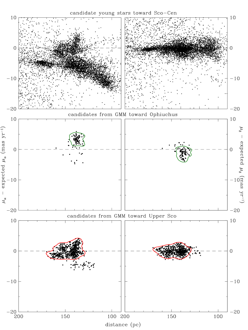
Figure 1.— Proper motion offsets versus parallactic distance for candidate young low-mass stars ($G_{\rm BP}-G_{\rm RP}$=1.4–3.4, $\sim$0.15–1 $M_{\odot}$) toward Sco-Cen (top). Candidate members of Sco-Cen have been identified by applying a GMM to these data. I have plotted the resulting candidates that are located within the boundary of Ophiuchus from Esplin et al. (2018) (middle) and the candidates that are outside of that boundary and within the triangular area in Upper Sco from Luhman & Esplin (2020) (bottom). I have included density contours that encompass the main concentration of candidates in each sample, which serve as criteria for selecting candidate members of these populations.

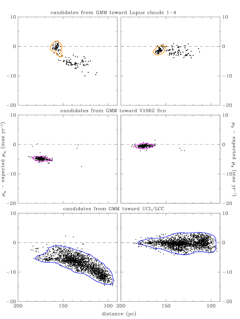
Figure 2.— Same as Figure 1 but for Lupus clouds 1–4 (top), the V1062 Sco group (middle), and UCL/LCC (bottom).

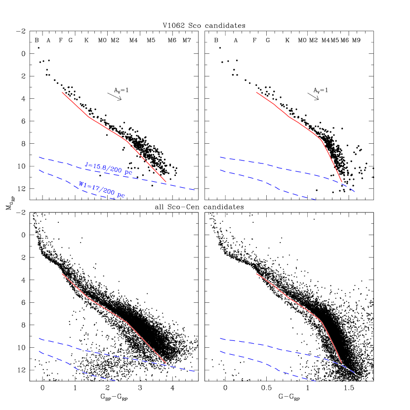
Figure 3.— $M_{G_{\rm RP}}$ versus $G_{\rm BP}-G_{\rm RP}$ and $G-G_{\rm RP}$ for candidate members of V1062 Sco within a radius of $2\arcdeg$ from the center of that group (top) and all candidate members of Sco-Cen (bottom) selected with the kinematic criteria in Figures 1 and 2. To further refine those kinematic candidates, I have defined boundaries that follow the lower envelopes of the sequences in V1062 Sco (red solid lines) and I have rejected candidates that appear below them unless they exhibit mid-IR excess emission, in which case they are retained. For reference, I have indicated the spectral types that correspond to the colors of young stars (Table 4) and I have marked the completeness limits for 2MASS and WISE in $J$ and W1, respectively, based on those colors and a distance of 200 pc, which is just beyond the far side of Sco-Cen (blue dashed lines).

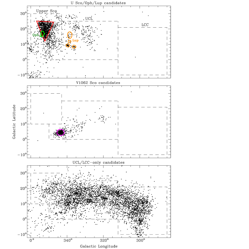
Figure 4.— Spatial distribution of candidate members of populations in Sco-Cen based on the kinematic and photometric criteria in Figures 1–3. I have marked the boundaries for Upper Sco, UCL, and LCC from de Zeeuw et al. (1999) (dashed lines), the boundary for Ophiuchus from Esplin et al. (2018) (green polygon), a field toward the center of Upper Sco defined by Luhman & Esplin (2020) (red triangle), the fields encompassing Lupus clouds 1–4 from Luhman (2020) (orange ellipses), and a $2\arcdeg$ radius field toward V1062 Sco (magenta ellipse).

Figure 5.— Histograms of $G_{\rm BP}-G_{\rm RP}$ and $G-G_{\rm RP}$ for the most reliable sample of Sco-Cen candidates (solid lines) and the estimated contamination from field stars (dotted lines). For each color, the candidates are required to have photometric errors of $<0.1$ mag in both bands, RUWE$<$1.6, $\sigma_{\pi}<0.5$ mas, and locations within the Sco-Cen boundaries from de Zeeuw et al. (1999).

Figure 6.— Equivalent widths of Li versus spectral type for candidate members of Ophiuchus, Lupus, Upper Sco, and UCL/LCC.

Figure 7.— Fraction of sources from Gaia EDR3 toward Sco-Cen that have RUWE$<$1.6, $\sigma_{\pi}<0.5$ mas, and $\sigma_{BP}<0.1/\sigma_{RP}<0.1$ or $\sigma_{G}<0.1/\sigma_{RP}<0.1$. The data in this diagram provide an estimate of the completeness of samples of candidates in Sco-Cen that are required to satisfy those criteria in order to reduce field star contamination (Sections 2.6 and 3.1).

Figure 8.— Top: Spatial distributions of stars from this work that have kinematics consistent with membership in Upper Sco or Ophiuchus (left) and candidate members of Ophiuchus from Grasser et al. (2021) that have $\sigma_{\pi}<1$ mas (right). I have marked the boundary for Ophiuchus from Esplin et al. (2018) (green polygon), a field toward the center of Upper Sco defined by Luhman & Esplin (2020) (red triangle), and contours for $A_{K}=0.5$ from the extinction map of Juvela & Montillaud (2016) (magenta curves). Bottom: Proper motion offsets versus parallactic distance for the candidates from Grasser et al. (2021) are shown with the thresholds from Figures 1 and 2 that are used in this work for selecting candidate members of populations in Sco-Cen.

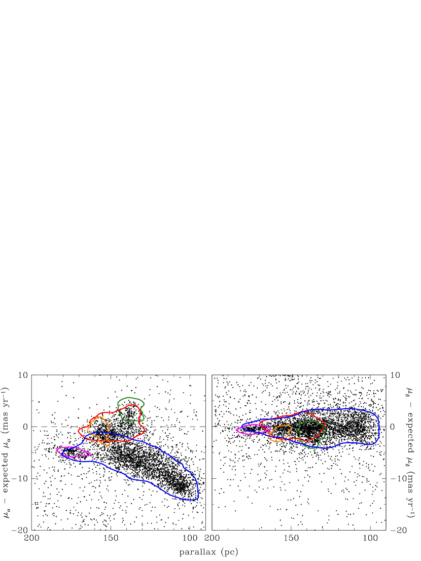
Figure 9.— Proper motion offsets versus parallactic distance for eRASS1 sources toward Sco-Cen from Schmitt et al. (2021) are shown with the thresholds from Figures 1 and 2 that are used in this work for selecting candidate members of populations in Sco-Cen.

Figure 10.— Count rate versus $G$ magnitude for eRASS1 sources from Schmitt et al. (2021) toward Sco-Cen (left) and an area within Sco-Cen toward Upper Sco (right). The typical flux limit adopted for Upper Sco in that study is indicated (dashed line).

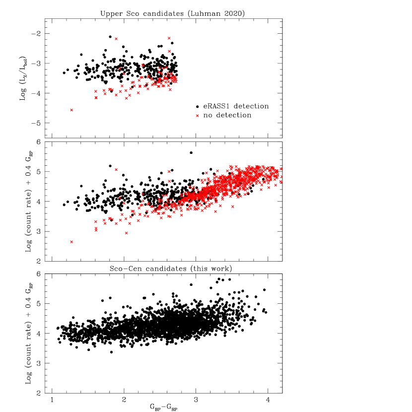
Figure 11.— Top: $L_{\rm X}/L_{\rm bol}$ versus $G_{\rm BP}-G_{\rm RP}$ for candidate members of Upper Sco from Luhman & Esplin (2020) based on eRASS1 data from Schmitt et al. (2021) and $G$-band bolometric corrections from Andrae et al. (2018). The latter are available for $T_{\rm eff}\gtrsim 3300$ K ($G_{\rm BP}-G_{\rm RP}\lesssim 2.7$). A limit of 0.056 counts s^-1 has been assumed for the nondetections. Middle: The candidates from Luhman & Esplin (2020) are plotted in terms of a ratio of X-ray and $G_{\rm RP}$ fluxes (in arbitrary units), which does not require a bolometric correction. Bottom: The same ratio is shown for candidate members of Sco-Cen from this work (Section 2.9).

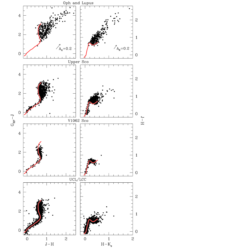
Figure 12.— $G_{\rm RP}-J$ versus $J-H$ and $J-H$ versus $H-K_{s}$ for candidate members of populations in Sco-Cen as defined in Section 3.1. The intrinsic colors of young stars from B0–M9 are indicated (red lines, Table 4).

Figure 13.— Histograms of spectral types for candidate members of Upper Sco, Ophiuchus ($A_{K}<0.5$), V1062 Sco, and UCL/LCC that satisfy the criteria in Section 3.1 (solid histograms). For stars that lack spectroscopy, spectral types have been estimated from photometry (Figure 12, Section 3.2). A second histogram is shown for Upper Sco that includes additional young stars that are absent from the Gaia sample and have been identified in spectroscopic surveys (dotted histogram, Luhman & Esplin, 2020, references therein). The arrows mark the spectral types that correspond to masses of 0.1 and 1 $M_{\odot}$ for ages of 10 Myr according to evolutionary models (e.g., Baraffe et al., 1998).

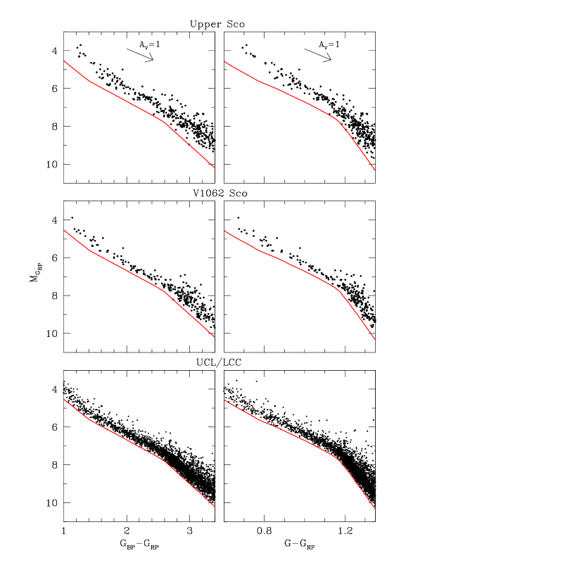
Figure 14.— $M_{G_{\rm RP}}$ versus $G_{\rm BP}-G_{\rm RP}$ and $G-G_{\rm RP}$ for candidate late-type ($\sim$K0–M5) members of Upper Sco, V1062 Sco, and UCL/LCC that have $\sigma_{\pi}<0.1$ mas and $A_{K}<0.1$ and do not have full disks. The boundaries from Figure 3 that were used for selecting candidates have been included (red lines).

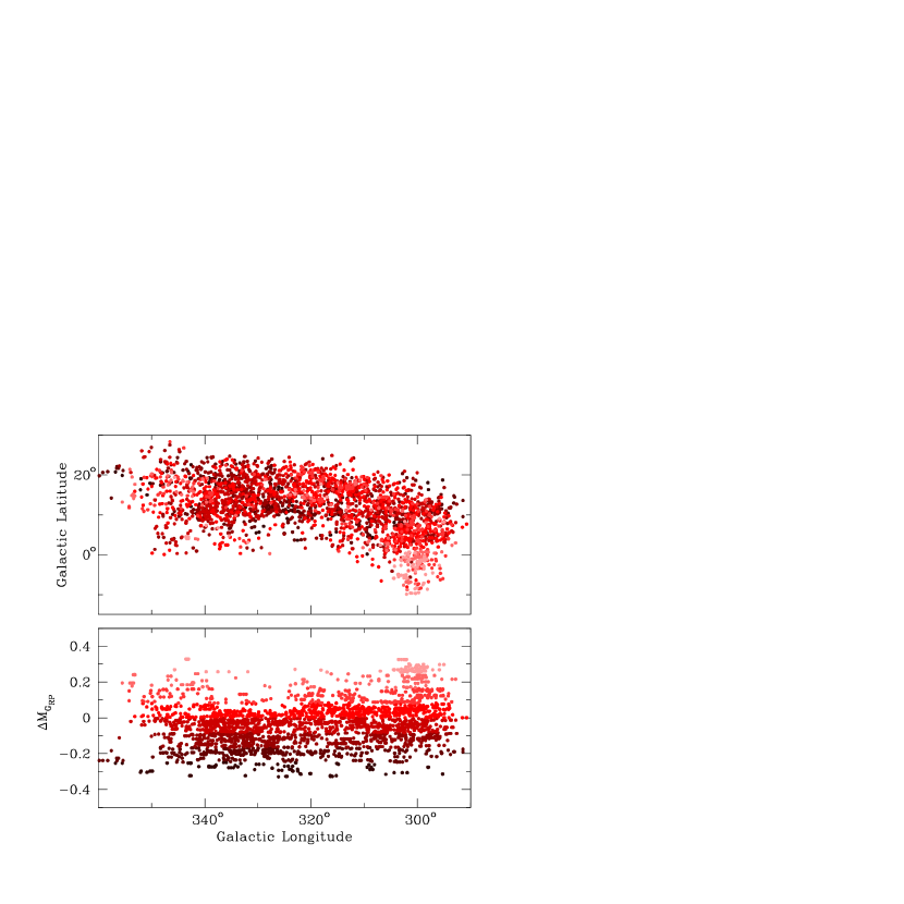
Figure 15.— Median offsets in $M_{G_{\rm RP}}$ from the median sequence of UCL/LCC for each candidate member of UCL/LCC from Figure 14 and its six closest neighbors in $XYZ$. The offsets are defined so that positive values correspond to younger ages. The colors of the points correspond to the values of the $M_{G_{\rm RP}}$ offsets.

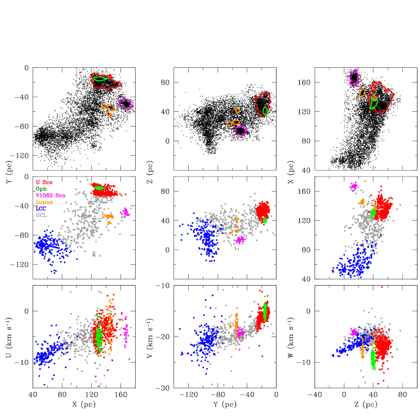
Figure 16.— Galactic Cartesian coordinates for candidate members of Sco-Cen (top). The density contours encompass most of the candidates within the fields marked in Figure 4 for Upper Sco, Ophiuchus, Lupus, and V1062 Sco. Candidates that have radial velocities are plotted in diagrams of $XYZ$ and $UVW$ (middle and bottom) if they are within those four fields and are kinematic members of those populations. In addition, kinematic members of UCL/LCC are plotted as blue points if they are within the boundary of LCC from de Zeeuw et al. (1999) and otherwise are plotted as gray points.

References

- Abt & Morrell (1995) Abt, H. A., & Morrell, N. I. 1995, ApJS, 99, 135
- Alcalá et al. (1995) Alcalá, J. M., Krautter, J., Schmitt, J. H. M. M., et al. 1995, A&AS, 114, 109
- Alcalá et al. (2020) Alcalá, J. M., Majidi, F. Z., Desidera, S., et al. 2020, A&A, 635, L1
- Alcalá et al. (2017) Alcalá, J. M., Manara, C. F., Natta, A., et al. 2017, A&A, 600, A20
- Alcalá et al. (2014) Alcalá, J. M., Natta, A., Manara, C. F., et al. 2014, A&A, 561, A2
- Allen et al. (2007) Allen, P. R., Luhman, K. L., Myers, P. C., et al. 2007, ApJ, 655, 1095
- Aller et al. (2013) Aller, K. M., Kraus, A. L., Liu, M. C., et al. 2013, ApJ, 773, 63
- Allers & Liu (2020) Allers, K. N., & Liu, M. C. 2020, PASP, 132, 104401
- Alonso et al. (2015) Alonso, R., Deeg, H. J., Hoyer, S., et al. 2015, A&A, 584, L8
- Alves de Oliveira et al. (2012) Alves de Oliveira, C., Moraux, E., Bouvier, J., & Bouy, H. 2012, A&A, 539, 151
- Alves de Oliveira et al. (2010) Alves de Oliveira, C., Moraux, E., Bouvier, J., et al. 2010, A&A, 515, 75
- Andersen & Nordstrom (1983) Andersen, J., & Nordstrom, B. 1983, A&AS, 52, 471
- Andrae et al. (2018) Andrae, R., Fouesneau, M., Creevey, O., et al. 2018, A&A, 616, A8
- Ansdell et al. (2016) Ansdell, M., Gaidos, E., Rappaport, S. A., et al. 2016, ApJ, 816, 69
- Appenzeller et al. (1983) Appenzeller, I., Jankovics, I., & Krautter, J. 1983, A&AS, 53, 291
- Ardila et al. (2000) Ardila, D., Martín, E., & Basri, G. 2000, AJ, 120, 479
- Bailer-Jones et al. (2021) Bailer-Jones, C. A. L., Rybizki, J., Fouesneau, M., Demleitner, M., & Andrae, R. 2021, AJ, 161, 147
- Baraffe et al. (1998) Baraffe, I., Chabrier, G., Allard, F., & Hauschildt, P. H. 1998, A&A, 337, 403
- Baraffe et al. (2015) Baraffe, I., Hormeier, D., Allard, F., & Chabrier, G. 2015, A&A, 577, 42
- Béjar et al. (2008) Béjar, V. J. S., Zapatero Osorio, M. R., Pérez-Garrido, A., et al. 2008, ApJ, 673, L185
- Bell et al. (2015) Bell, C. P. M., Mamajek, E. E., & Naylor, T. 2015, MNRAS, 454, 593
- Biazzo et al. (2017) Biazzo, K., Frasca, A., Alcalá, J. M., et al. 2017, A&A, 605, A66
- Bildsten et al. (1997) Bildsten, L., Brown, E. F., Matzner, C. D., & Ushomirsky, G. 1997, ApJ, 442
- Binks & Jeffries (2016) Binks, A. S., & Jeffries, R. D. 2016, MNRAS, 455, 3345
- Blaauw (1964) Blaauw, A. 1964, ARA&A, 2, 213
- Blondel & Tjin A Djie (2006) Blondel, P. F. C., & Tjin A Djie, H. R. E. 2006, A&A, 456, 1045
- Bonnefoy et al. (2014) Bonnefoy, M., Chauvin, G., Lagrange, A.-M., et al. 2014, A&A, 562, A127
- Bouvier & Appenzeller (1992) Bouvier, J., & Appenzeller, I. 1992, A&AS, 92, 481
- Bowler et al. (2019) Bowler, B. P., Hinkley, S., Ziegler, C., et al. 2019, ApJ, 877, 60
- Bowler et al. (2014) Bowler, B. P., Liu, M. C., Kraus, A. L., & Mann, A. W. 2014, ApJ, 784, 65
- Bragança et al. (2012) Bragança, G. A., Dalton, S., Cunha, K., et al. 2012, AJ, 144, 130
- Brandner et al. (1997) Brandner, W., & Zinnecker, H. 1997, A&A, 321, 220
- Budding et al. (2015) Budding, E., Butland, R., & Blackford, M. 2015, MNRAS, 448, 3784
- Buder et al. (2021) Buder, S., Sharma, S., Kos, J., et al. 2021, MNRAS, 506, 150
- Buscombe (1969) Buscombe, W. 1969, MNRAS, 144, 31
- Cannon & Pickering (1993) Cannon, A. J., & Pickering, E. C. 1993, yCat, 3135, 0
- Cánovas et al. (2019) Cánovas, H., Cantero, C., Cieza, L., et al. 2019, A&A, 626, A80
- Cantat-Gaudin et al. (2019) Cantat-Gaudin, T., Jordi, C., Wright, N. J., et al. 2019, A&A, 626, A17
- Carpenter et al. (2006) Carpenter, J. M., Mamajek, E. E., Hillenbrand, L. A., & Meyer, M. R. 2006, ApJ, 651, L49
- Chen et al. (2005) Chen, C. H., Jura, M., Gordon, K. D., & Blaylock, M. 2005, ApJ, 623, 493
- Chen et al. (2011) Chen, C. H., Mamajek, E. E., Bitner, M. A., et al. 2011, AJ, 738, 122
- Chen et al. (2012) Chen, C. H., Pecaut, M., Mamajek, E. E., Su, K. Y. L., & Bitner, M. A. 2012, ApJ, 756, 133
- Choi et al. (2016) Choi, J., Dotter, A., Conroy, C., et al. 2016, ApJ, 823, 102
- Cieza et al. (2007) Cieza, L., Padgett, D. L., Stapelfeldt, K. R., et al. 2007, ApJ, 667, 308
- Cieza et al. (2010) Cieza, L. A., Schreiber, M. R., Romero, G. A., et al. 2010, ApJ, 712, 925
- Close et al. (2007) Close, L. M., Zuckerman, B., Song, I., et al. 2007, ApJ, 660, 1492
- Cody et al. (2017) Cody, A. M., Hillenbrand, L. A., David, T. J., et al. 2017, ApJ, 836, 41
- Cohen & Kuhi (1979) Cohen, M., & Kuhi, L. V. 1979, ApJS, 41, 743
- Cohen et al. (1986) Cohen, M., Dopita, M. A., & Schwartz, R. D. 1986, ApJ, 307, L21
- Comerón (2008) Comerón, F. 2008, in Handbook of Star Forming Regions, Vol. 2, The Southern Sky, ASP Monograph Series 5, ed. B. Reipurth (San Francisco, CA: ASP), 295
- Comerón et al. (2003) Comerón, F., Fernández, M., Baraffe, I., Neuhäuser, R., & Kaas, A. A. 2003, A&A, 406, 1001
- Comerón et al. (2013) Comerón, F., Spezzi, L., López Martí, B., & Merín, B. 2013, A&A, 554, A86
- Cook et al. (2017) Cook, N. J., Scholz, A., & Jayawardhana, R. 2017, AJ, 154, 256
- Corbally (1984) Corbally, C. J. 1984, ApJS, 55, 657
- Covino et al. (1997) Covino, E., Alcala, J. M., Allain, S., Bouvier, J., Terranegra, L., & Krautter, J. 1997, A&A, 328, 187
- Cruz et al. (2003) Cruz, K. L., Reid, I. N., Liebert, J., Kirkpatrick, J. D., & Lowrance, P. J. 2003, AJ, 126, 2421
- Cutispoto et al. (2002) Cutispoto, G., Pastori, L., Pasquini, L., et al. 2002, A&A, 384, 491
- Cutri et al. (2012) Cutri, R. M., Wright, E. L., Conrow, T., et al. 2012, yCat, 2311, 0C
- Cutri et al. (2013a) Cutri, R. M., Wright, E. L., Conrow, T., et al. 2013a, yCat, 2328, 0C
- Cutri et al. (2013b) Cutri, R. M., Wright, E. L., Conrow, T., et al. 2013b, Explanatory Supplement to the AllWISE Data Release Products, http://wise2.ipac.caltech.edu/docs/release/allwise/expsup/index.html
- Dahm et al. (2012) Dahm, S. E. Slesnick, C. L., & White, R. J. 2012, ApJ, 745, 56
- Damiani et al. (2019) Damiani, F., Prisinzano, L., Pillitteri, I., Micela, G., & Sciortino, S. 2019, A&A, 623, A112
- David et al. (2016a) David, T. J., Hillenbrand, L. A., Cody, A. M., Carpenter, J. M., & Howard, A. W. 2016a, ApJ, 816, 21
- David et al. (2019) David, T. J., Hillenbrand, L. A., Gillen, E., et al. 2019, ApJ, 872, 161
- David et al. (2016b) David, T. J., Hillenbrand, L. A., Petigura, E. A., et al. 2016b, Nature, 534, 658
- Dawson et al. (2014) Dawson, P., Scholz, A., Ray, T. P., et al. 2014, MNRAS, 442, 1586
- de Bruijne (2012) de Bruijne, J. H. J. 2012, Ap&SS, 341, 31
- de Geus et al. (1989) de Geus, E. J., de Zeeuw, P. T., & Lub, J. 1989, A&A, 216, 44
- Desidera et al. (2015) Desidera, S., Covino, E., Messina, S., et al. 2015, A&A, 573, A126
- de Zeeuw et al. (1999) de Zeeuw, P. T., Hoogerwerf, R., de Bruijne, J. H. J., Brown, A. G. A., & Blaauw, A. 1999, AJ, 117, 354
- Dotter (2016) Dotter, A. 2016, ApJS, 222, 8
- Edwards (1976) Edwards, T. W. 1976, AJ, 81, 245
- Eisner et al. (2005) Eisner, J. A., Hillenbrand, L. A., White, R. J., Akeson, R. L., & Sargent, A. I. 2005, ApJ, 623, 952
- Eisenhardt et al. (2020) Eisenhardt, P. R. M., Marocco, F., Fowler, J. W., et al. 2020, ApJS, 247, 69
- Erickson et al. (2011) Erickson, K. L., Wilking, B. A., Meyer, M. R., Robinson, J. G., & Stephenson, L. N. 2011, AJ, 142, 140
- Esplin & Luhman (2019) Esplin, T. L., & Luhman, K. L. 2019, AJ, 158, 54
- Esplin & Luhman (2020) Esplin, T. L., & Luhman, K. L. 2020, AJ, 160, 44
- Esplin & Luhman (2021) Esplin, T. L., & Luhman, K. L. 2021, AJ, submitted
- Esplin et al. (2017) Esplin, T. L., Luhman, K. L., Faherty, J. K., Mamajek, E. E., & Bochanski, J. J. 2017, AJ, 154, 46
- Esplin et al. (2018) Esplin, T. L., Luhman, K. L., Miller, E. B., & Mamajek, E. E. 2018, AJ, 156, 75
- Fabricius et al. (2021) Fabricius, C., Luri, X., Arenou, F., et al. 2021, A&A, 649, A5
- Fan et al. (2017) Fang, M., Kim, J. S., Pascucci, I., et al. 2017, AJ, 153, 188
- Feiden (2016) Feiden, G. A. 2016, A&A, 593, A99
- Feigelson & Lawson (2004) Feigelson, E. D., & Lawson, W. A. 2004, ApJ, 614, 267
- Feigelson & Montmerle (1999) Feigelson, E. D., & Montmerle, T. 1999, ARA&A, 37, 363
- Feigelson et al. (2013) Feigelson, E. D., Townsley, L. K., Broos, P. S., et al. 2013, ApJS, 209, 26
- Finkenzeller & Basri (1987) Finkenzeller, U., & Basri, G. 1987, ApJ, 318, 823
- Frasca et al. (2017) Frasca, A., Biazzo, K., Alcalá, J. M., et al. 2017, A&A, 602, A33
- Gagné et al. (2015) Gagné, J., Faherty, J. K., Cruz, K. L., et al. 2015, ApJS, 219, 33
- Gahm et al. (1983) Gahm, G. F., Ahlin, P., & Lindroos, K. P. 1983, A&AS, 51, 143
- Gaia Collaboration et al. (2021) Gaia Collaboration, Brown, A. G. A., Vallenari, A., Prusti, T., et al. 2021, A&A, 649, A1
- Gaia Collaboration et al. (2016) Gaia Collaboration, Prusti, T., de Bruijne, J. H. J., et al. 2016, A&A, 595, A1
- Galli et al. (2013) Galli, P. A. B., Bertout, C., Teixeira, R., & Ducourant, C. 2013, A&A, 558, A77
- Galli et al. (2020) Galli, P. A. B., Bouy, H., Olivares, J., et al. 2020, A&A, 643, 148
- Garrison (1994) Garrison, R. F., & Gray, R. O. 1994, AJ, 107, 1556
- Gatti et al. (2006) Gatti, T., Testi, L., Natta, A., Randich, S., & Muzerolle, J. 2006, A&A, 460, 547
- Geers et al. (2007) Geers, V. C., Van Dishoeck, E. F., Visser, R., et al. 2007, A&A, 476, 279
- Getman et al. (2017) Getman, K. V., Broos, P. S., Kuhn, M. A., et al. 2017, ApJS, 229, 28
- Getman et al. (2002) Getman, K. V., Feigelson, E. D., Townsley, L., et al. 2002, ApJ, 575, 354
- Gizis (2002) Gizis, J. E. 2002, ApJ, 575, 484
- Glaspey (1972) Glaspy, J. W. 1972, AJ, 77, 474
- Goldman et al. (2018) Goldman, B., Röser, S., Schilbach, E., Moór, A. C., & Henning, T. 2018, ApJ, 868, 32
- Gontcharov (2006) Gontcharov, G. A. 2006, AstL, 32, 759
- Grasser et al. (2021) Grasser, N., Ratzenböck, S., Alves, J., et al. 2021, A&A, 652, A2
- Gregory et al. (2016) Gregory, S. G., Adams, F. C., & Davies, C. L. 2016, MNRAS, 457, 3836
- Greene & Meyer (1995) Greene, T. P. & Meyer, M. R. 1995, ApJ, 450, 233
- Grosso et al. (2000) Grosso, N., Montmerle, T., Bontemps, S., André, Ph., & Feigelson, E. 2000, A&A, 359, 113
- Güdel et al. (2007) Güdel, M., Briggs, K. R., Arzner, K., et al. 2007, A&A, 468, 353
- Guenther et al. (2001) Guenther, E. W., Torres, G., Stout-Batalha, N. M., et al. 2001, A&A, 366, 965
- Gutiérrez Albarrán et al. (2020) Gutiérrez Albarrán, M. L., Montes, D. Gómez Garrido, M., et al. A&A, 643, A71
- Herbig (1977) Herbig, G. H. 1977, ApJ, 214, 747
- Herczeg et al. (2009) Herczeg, G. J., Cruz, K. L., & Hillenbrand, L. A. 2009, ApJ, 696, 1589
- Herczeg & Hillenbrand (2014) Herczeg, G. J., & Hillenbrand, L. A. 2014, ApJ, 786, 97
- Heyer & Graham (1989) Heyer, M. H., & Graham, J. A. 1989, PASP, 101, 816
- Heyer & Graham (1990) Heyer, M. H., & Graham, J. A. 1990, PASP, 102, 117
- Hiltner et al. (1969) Hiltner, W. A., Garrison, R. F., & Schild, R. E. 1969, ApJ, 157, 313
- Hinkley et al. (2015) Hinkley, S., Kraus, A. L., Ireland, M. J., et al. 2015, ApJ, 806, L9
- Hoogerwerf (2000) Hoogerwerf, R. 2000, MNRAS, 313, 43
- Houk (1975) Houk, N. 1975, Michigan Catalogue of Two-dimensional Spectral Types for the HD Stars. Vol. 1, (Ann Arbor: Univ. Mich.)
- Houk (1978) Houk, N. 1978, Michigan Catalogue of Two-dimensional Spectral Types for the HD Stars. Vol. 2, (Ann Arbor: Univ. Mich.)
- Houk (1982) Houk, N. 1982, Michigan Catalogue of Two-dimensional Spectral Types for the HD Stars. Vol. 3, (Ann Arbor: Univ. Mich.)
- Houk & Smith-Moore (1988) Houk, N., & Smith-Moore, M. 1988, Michigan Catalogue of Two-dimensional Spectral Types for the HD Stars. Vol. 4, (Ann Arbor: Univ. Mich.)
- Houk & Swift (1999) Houk, N., & Swift, C. 1999, Michigan Catalogue of Two-dimensional Spectral Types for the HD Stars. Vol. 5, (Ann Arbor: Univ. Mich.)
- Hughes et al. (1994) Hughes, J., Hartigan, P., Krautter, J., & Kelemen, J. 1994, AJ, 108, 1071
- Indebetouw et al. (2005) Indebetouw, R., Mathis, J. S., Babler, B. L., et al. 2005, ApJ, 619, 931
- James et al. (2006) James, D. J., Melo, C., Santos, N. C., & Bouvier, J. 2006, A&A, 446, 971
- Janson et al. (2012) Janson, M., Jayawardhana, R., Girard, J. H., et al. 2012, ApJ, 758, L2
- Janson et al. (2013) Janson, M., Lafrenière, D., Jayawardhana, R., et al. 2013, ApJ, 773, 170
- Jayawardhana & Ivanov (2006) Jayawardhana, R., & Ivanov, V. D. 2006, ApJ, 647, L167
- Jilinski et al. (2006) Jilinksi, E., Daflon, S., Cunha, K., & de La Reza, R. 2006, A&A, 448, 1001
- Johnson & Soderblom (1987) Johnson D. R. H., & Soderblom D. R., 1987, AJ, 93, 864
- Jönsson et al. (2020) Jönsson, H., Holtzman, J. A., Prieto, C. A., et al. 2020, AJ, 160, 120
- Juvela & Montillaud (2016) Juvela, M., & Montillaud, J. 2016, A&A, 585, A38
- Kahraman Aliçavuş et al. (2016) Kahraman Aliçavuş, F., Niemczura, E., De Cat, P., et al. 2016, MNRAS, 458, 2307
- Kerr et al. (2021) Kerr, R., Rizzuto, A. C., Kraus, A. L., & Offner, S. S. R. 2021, ApJ, 917, 23
- Koen et al. (2017) Koen, C., Miszalski, B., Väisänen, P., & Koen, T. 2017, MNRAS, 465, 4723
- Kounkel et al. (2018) Kounkel, M., Covey, K., Suárez, G., et al. 2018, AJ, 156, 84
- Kraus et al. (2015) Kraus, A. L., Cody, A. M., Covey, K. R., et al. 2015, ApJ, 807, 3
- Kraus & Hillenbrand (2007) Kraus, A. L., & Hillenbrand, L. A. 2007, ApJ, 664, 1167
- Kraus & Hillenbrand (2009) Kraus, A. L., & Hillenbrand, L. A. 2009, ApJ, 703, 1511
- Krautter et al. (1997) Krautter, J., Wichmann, R., Schmitt, J. H. M. M., et al. 1997, A&AS, 123, 329
- Kuhn et al. (2019) Kuhn, M. A., Hillenbrand, L. A., Sills, A., Feigelson, E. D., & Getman, K. V. 2019, ApJ, 870, 32
- Kunder et al. (2017) Kunder, A., Kordopatis, G., Steinmetz, M., et al. 2017, AJ, 153, 75
- Kunkel (1999) Kunkel, M. 1999, Ph.D. thesis, Julius-Maximilians-Univ., Wuürzburg
- Kurosawa et al. (2006) Kurosawa, R., Harries, T. J., & Littlefair, S. P. 2006, MNRAS, 372, 1879
- Lachapelle et al. (2015) Lachapelle, F.-R., Lafrenière, D., Gagné, J., et al. 2015, ApJ, 802, 61
- Levato (1975) Levato, H. 1975, A&AS, 19, 91
- Levenhagen & Leister (2006) Levenhagen, R. S., & Leister, N. V. 2006, MNRAS, 371, 252
- Lindegren (2018) Lindegren, L. 2018, Re-normalising the astrometric chi-square in Gaia EDR3, GAIA-C3-TN-LU-LL-124-01, http://www.rssd.esa.int/doc_fetch.php?id=3757412
- Lodieu et al. (2015) Lodieu, N., Alonso, R., González Hernández, J. I., et al. 2015, A&A, 584, A128