Analogue Radio over Fiber aided Multi-service Communications for High Speed Trains

Yichuan Li, Salman Ghafoor, Mohammed El-Hajjar, Senior Member, IEEE
Y. Li is with Harbin Institute of Technology (Shenzhen), Shenzhen, China (e-mail: liyichuan@hit.edu.cn).S. Ghafoor is with the National University of Sciences and Technology, Pakistan (e-mail: salman.ghafoor@seecs.edu.pk).M. El-Hajjar is with the School of Electronics and Computer Science, University of Southampton, SO17 1BJ, United Kingdom (meh@ecs.soton.ac.uk).

Abstract

High speed trains (HST) have gradually become an essential means of transportation, where given our digital world, it is expected that passengers will be connected all the time. More specifically, the on-board passengers require fast mobile connections, which cannot be provided by the currently implemented cellular networks. Hence, in this article, we propose an analogue radio over fiber (A-RoF) aided multi-service network architecture for high-speed trains, in order to enhance the quality of service as well as reduce the cost of the radio access network (RAN). The proposed design can simultaneously support sub-6GHz as well as milimeter wave (mmWave) communications using the same architecture. Explicitly, we design a photonics aided beamforming technique in order to eliminate the bulky high-speed electronic phase-shifters and the hostile broadband mmWave mixers while providing a low-cost RAN solution. Finally, a beamforming range of 180^∘ is demonstrated with a high resolution using our proposed system.

Index Terms:

Optical fiber, radio access network, Beyond 5G, High speed train, analogue radio over fiber, mmWave beamforming.

I Introduction

The high speed train (HST) operating at a speed above 300 km/hour has fundamentally changed the individuals’ life-style. It is reported that HST has the second-highest internet streaming after household environments, such as homes and offices [1, 2], where the majority of this streaming is used for supporting the on-board activities, such as on-demand video, online-gaming, and voice or video calling. Furthermore, since the 4G and 5G use the sub-6GHz band and then the millimeter wave (mmWave) communications will coexist with these frequency bands [3], a railway network supporting multi-service is required, where the passengers are capable of being connected to 4G, 5G, Beyond 5G or even Wi-Fi networks all the time [4, 3, 5]. On the other hand, HST requires high capacity due to the increasingly high number of passengers and the severe Doppler effects caused by the high speed [6, 7]. As a result, this requires more base-stations and an efficient cellular handover technique, which has several challenges [6, 7, 8, 9]. First, the denser deployment of base stations (BS) can provide seamless connection for the passengers by increasing the capacity per cell, which by contrary would impose more inter-cell interference (ICI) [6, 7]. Then, the severe Doppler effects seriously undermine the system as the train is moving extremely fast, impacting the handover process of the cellular networks [4, 5]. Besides, the channel estimation might not be accurate due to the rapid channel variations, influencing the quality of service (QoS) and hence, the user experience [8, 9].

Refer to caption — Figure 1: Multi-service HST System Architecture

As a solution, mmWave beamforming has been proposed for mitigating the ICI, while enhancing the capacity, especially in ultra-dense cellular networks [10]. On the other hand, two-hop relay communications are advocated by [1, 4] to address the handover failure and the rapid channel variation in HSTs, where several relay antennas can be installed on the rooftop of the train cars for a stable handover. However, in order to have a decent quality of service (QoS), a large number of base-stations must be deployed, increasing the total cost of the radio access networks (RANs) including both the Capital Expenditure (CAPEX) and the Operational Expenditure (OPEX). Hence, ultra-light RANs are required [11]. In addition, mmWave communications beamforming requires high-speed mmWave phase-shifters [12], which increases the overall RAN cost and limits the tuning carrier frequency range [13, 14, 15], and the broadband mixers, which affects achievable the bit error rate (BER) performance [13]. Furthermore, the phase-shifter based beamforming would impose beam-squinting on the wideband signals¹¹1Beamsquinting is the beam-shifts caused by the frequency shifts when applied with the constant phase-shift among neighbouring antenna element (AE). This would be even severe in the context of wide-band signal beamsteering [15]..

The analogue radio over (A-RoF) based true-time delay is a low-cost yet high-performance RAN solution with ultra-light remote radio head (RRH) [16, 6, 17, 18, 19, 14, 20], where the RAN is separated between the central unit (CU) and several RRHs and is capable of reducing both its power-consumption and complexity. Explicitly, the A-RoF aided beamformer was proposed for providing beam-squinting free beamforming using the uniform fiber Bragg grating (FBG) [15, 21, 22] or a single chirped FBG (CFBG) [23, 24].

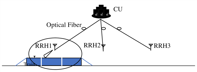
In this article, we design a two-hop HST communications network combined with the A-RoF aided beamforming techniques, where multi services, such as on-demand video, online-gaming, and voice or video calling, which are carried by mmWave and sub-6GHz signals using 4G, 5G or Wi-Fi networks are delivered to the train. Explicitly, the multi service signals generated in the CU of Fig. 1 are transmitted through a short-length fiber of upto 20km to the RRHs, which communicate with the antennas on the top of the HST to provide the required service to the on-board passengers. The beam pattern is controlled in the CU using the CFBG, instead of the costly and bulky phase-shifters in the RRHs, alleviating the size and cost of the RRH and facilitating the densely deployed RRHs along the railways. The proposed system enables both cost-reduction by simplifying the RAN design and performance-improvement by exploiting centralised optical processing and multi-service signal generation as a benefit of the A-RoF architecture [14]. The novel contributions of our system are as follow:

1.

Photonic aided true-time delay beamforming: We conceive a multi-service true-time-delay transmit beamforming for HST two-hop network, while also eliminating the beam-squinting phenomenon.
2.

Energy-efficient RRHs: The large-scale power-thirsty phase shifters and costly mmWave phase shifters are removed, while the beam is optically controlled using the passive FBGs in the proposed design, hence improving the OPEX-savings and enabling ultra-light RRHs deployment.
3.

Multi-service signal generation: multi-service signals carried by mmWave and sub-6GHz frequency band can be optically generated and beam-steered to the HST in the same direction.
4.

Centralised optical processing: unlike the phase-shifter used in conventional wireless transmit beamforming, the beam control module is located in the central unit, potentially facilitating the coordinated multipoint (CoMP) transmission.

The rest of the paper is organised as follows. We introduce the multi-service two-hop train system in Section II, while the A-RoF aided beamforming technique and its time delay principle are detailed in Section III. Then, we present the cost-benefits and the beamforming performance of our proposed system in Section IV, followed by the conclusion in Section V.

II Multi-service HST System Architecture

In this section, we present a general architecture for the two-hop HST system shown in Fig. 1, which can be exploited in our design. As shown in Fig. 1, the signal is generated in the CU and transmitted via fiber to several RRHs, where only optical-to-electronic conversion, amplification and filtering are performed, thus substantially reducing the RRH size. Explicitly, the RRH receives the signal from the CU using fiber and then transmits this signal to the HST using a set of antenna arrays, as shown in Fig. 1, where the RRHs are placed along the train line and will communicate with the antenna arrays on the rooftop of the HST.

The signals transmitted from the RRHs to the HST are beamformed and transmitted to the antenna arrays fixed on the rooftop of the HST, as shown in Fig. 1. Then, the signals are relayed to the on-board passengers to fulfill the users demands through the indoor communication system [25]. It has been verified using field tests that the two-hop relay communication in HST setup outperforms the conventional 4G cellular system in terms of signal quality [25].

Since the 4G and 5G signals would co-exist in the non-standalone 5G deployment proposed by the 3GPP in the recent Releases [26], multi-service signal transmission using different frequency bands and wireless standards are of importance to support the users’ daily streaming, on-line gaming, voice or video call and on-demand video [3].

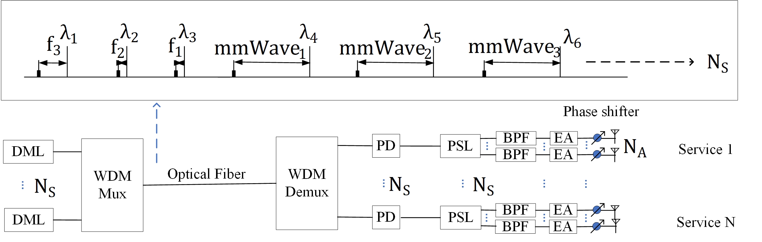
Conventionally, the A-RoF aided multi-service system can be supported using the architecture of Fig. 2 [1, 4, 9, 27, 25], where different services carried by different frequencies are directly modulated by individual lasers before being coupled into an optical fiber. At the end of the fiber, each optical and radio frequency (RF) chain are used for optical-to-electronic conversion, amplification, filterings. Furthermore, when analogue beamforming is employed for improving the signal-to-noise ratio performance, a large number of phase-shifters, band-pass filter (BPFs), electronic amplifiers (EAs) are required, which increases the cost and power-consumption of the whole system. Explicitly, let us take service 1 as an example, as shown in Fig. 2, assuming the RF of $f_{3}$ carries service 1, $f_{3}$ is used to directly modulate a laser operating at the center wavelength of $\lambda_{1}$ . Then, coupled with other services carried by $\lambda_{2}$ to $\lambda_{6}$ into the fiber, the wavelength division multiplexing (WDM) signal of the spectrum shown in Fig. 2 feeds the optical fiber for transmission, after which the WDM Demultiplexer (WDM Demux) separates each wavelength. Then, the modulated optical signal of $\lambda_{1}$ is photo-detected and the $f_{3}$ carrying service 1 is recovered, followed by the power splitter (PSL) which splits the power of the RF frequency, where, each BPF and EA is used for filtering out the wanted signal and for the amplification of each port of the PSL, respectively. Finally, several phase-shifters are used to phase-shift each output to form a desired beam pattern, leading to the analogue beamforming with large amount of power-thirsty and bulky phase-shifter deployment. In the next section, we will introduce our A-RoF system based on the two-hop transmission, while invoking a lower-cost photonic aided multi-service solution.

III A-RoF aided Beamforming for High-speed Train Multi-service Communications

III-A A-RoF aided HST System Model

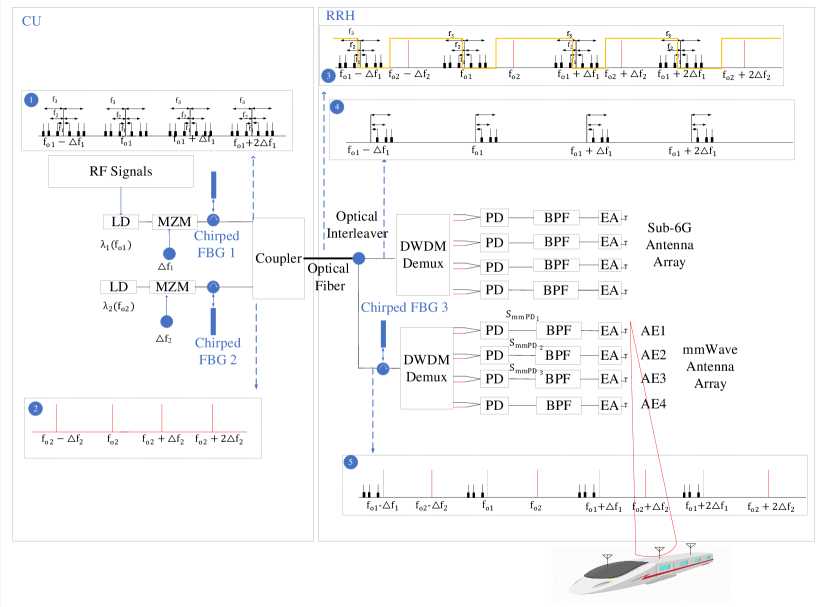
As mentioned in section II, the RRH beamforms the multi-service signals, composed of sub-6GHz and mmW signals, to the HST rooftop antenna arrays. Fig. 3 shows the proposed A-RoF design, where the sub-6GHz and mmW signals are beamformed in the same direction to the antenna array placed on the rooftop of the train. The proposed design avoids the beam-squinting as well as considers low-complexity RRH.

In Fig. 3, the access network is divided into CU and RRH, where the CU performs the baseband signal processing as well as the radio modulations [14], while the RRH is simplified to only radio functions such as amplifications and filtering. Explicitly, in the CU of Fig. 3, the RF signals of $f_{1}$ , $f_{2}$ and $f_{3}$ ²²2The number of frequencies can be readily extended, which depends on the bandwidth of the LD. directly modulate a laser diode (LD) operating at $\lambda_{1}$ . The signal at the output of the directly modulated laser is given at the optical input of a Mach-Zehnder modulator (MZM) that is being driven by a sinusoidal signal of frequency $\Delta f1$ . The nonlinear transfer function of the MZM results in the generation of multiple spectral copies of the directly modulated optical signal that have a frequency spacing of $\Delta f_{1}$ as shown in Fig. 3 [13]. The resulting WDM signal is time-delayed using a CFBG, which is capable of reflecting different wavelengths with a linear time-delay. Then, as shown in Fig. 3, another laser diode operating at $\lambda_{2}$ is intensity modulated by a sinusoidal signal having frequency of $\Delta f_{2}$ through a MZM to generate multiple sidebands by using the nonlinear function of the MZM [13]. The two WDM signals are coupled into a single mode fiber using a fiber coupler.

As shown in the RRH of Fig. 3, the combined WDM signal is separated by a two-port optical interleaver, which filters the desired signals to two individual dense wavelength division demultiplexers (DWDM Demux), each of which would be used for either sub-6GHz signal generation or mmWave signal generation. The upper DWDM Demux of Fig. 3 filters the spectrum which can generate a beat frequency of sub-6GHz bands. Then, the photodetected sub-6GHz frequency after each PD is band-pass filtered and amplified, while the inter-element time delay is dependent on the chirped FBG 1 and FBG 2 strains as tested by [28]. Similarly, the bottom DWDM Demux in the RRH of Fig. 3 is used for mmWave signal generation, where an extra chirped FBG, namely chirped FBG 3 of Fig. 3, is implemented for adjusting the beam direction to be the same as the sub-6GHz bands, which will be elaborated in the next section.

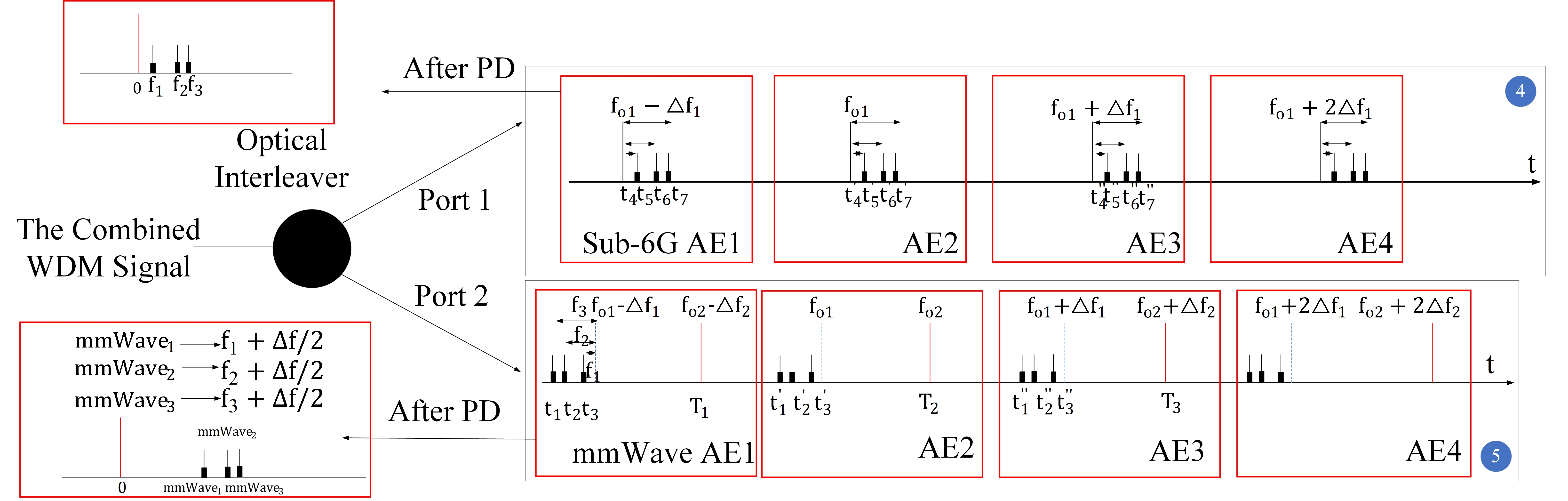
To elaborate further on the RF and mmWave signals generation, as shown in Fig. 4, the optical interleaver, which is a periodic optical filter, separates the combined WDM signals of spectrum ③ of Fig. 3. The spectrum of the two outputs of the optical interleaver is depicted in Fig. 4, where port 1 maps the spectrum ④ of Fig. 4 to the sub-6GHz spectrum of $f_{1}$ , $f_{2}$ and $f_{3}$ , with port 2 mapping the spectrum ⑤ to the mmWave frequencies of $f_{1}+\frac{\Delta f}{2}$ , $f_{2}+\frac{\Delta f}{2}$ and $f_{3}+\frac{\Delta f}{2}$ ³³3Note that if $\frac{\Delta f}{2}=f_{o1}-f_{o2}$ is upto 25 GHz, $f_{1}+\frac{\Delta f}{2}$ is the mmWave signal of at least 25 GHz. The spectrum ④ and ⑤ of Fig. 4 corresponds to spectrum ④ and ⑤ of Fig. 3.. Let us now consider a four-antenna-element system for both the sub-6GHz and mmWave transmission. The beating frequencies of the red boxes of Fig. 4 would be mapped to antenna elements 1-4 of both the mmWave antenna array and the sub-6GHz antenna array dispensing with the mmWave mixers and phase shifters, since they have been performed using the above optical link with the aid of WDM signal and CFBG.

Thus, a multi-service communication system transporting sub-6GHz and mmWave signals in the same direction is built for the two-hop HST systems. In the next section, we will detail the true-time delay principles and its mapping rule from the optical domain to the electronic domain as well as the multi-service generation.

III-B True-time Delay Principle

Instead of exploiting the conventional phase-shifting schemes for analogue beamforming [29], our proposed system invokes the true-time delay, which relies on the constant time-delay among the RF signal fed into the adjacent antennas elements to introduce the beam steering, which is capable of mitigating the wide-band beam-squinting problems [15]. While undermining the codebook design of the phased-array systems [30], beam-squinting is also detrimental for the channel estimation and precoding, which further degrades the wireless communication transmission rate [31].

In the following, with the aid of the mathematical derivation, we will prove how the imposed optical linear time-delay is used for introducing the constant time-delay among the RF signal fed into the adjacent antennas elements of each antenna array of Fig. 3. In the upper line of the CU in Fig. 3, where the spectrum ① is generated, the multi-service RF signals are used to directly modulate a laser diode and the input optical field of the MZM can be formulated as [13]:

E_{in}(t)=\sqrt{P_{Laser}}e^{j\omega_{\lambda_{1}}t}[1+cos(\omega_{f_{1}}t)+cos(\omega_{f_{2}}t)+cos(\omega_{f_{3}}t)],

(1)

where $P_{Laser}$ is the LD output power and $\omega_{f_{1}}$ , $\omega_{f_{2}}$ and $\omega_{f_{3}}$ denote the optical carrier’s angular frequency corresponding to $\lambda_{1}$ , $\lambda_{2}$ and $\lambda_{3}$ of Fig. 3. Then, the MZM output field [13] is as follows:

\begin{array}[]{lcl}E_{MZM_{up}}(t)\\ =cos(\pm\frac{\pi}{4}+\frac{\pi V_{dr}cos(\omega_{\Delta f_{1}})}{2V_{\pi}})E_{in}(t)\\ =\frac{\sqrt{P_{laser}}[1+cos(\omega_{f_{1}}t)+cos(\omega_{f_{2}}t)+cos(\omega_{f_{3}}t)]e^{j\omega_{\lambda_{1}}t}}{\sqrt{2}}[J_{0}(\frac{\pi|V_{dr}|}{2V_{\pi}})\\ +2\sum_{n=1}^{\infty}(-1)^{n}J_{2n}(\frac{\pi V_{dr}}{2V_{\pi}})cos(2n\omega_{\Delta f_{1}}t)\\ \pm 2\sum_{n=1}^{\infty}(-1)^{n}J_{2n-1}(\frac{\pi V_{dr}}{2V_{\pi}})cos((2n-1)\omega_{\Delta f_{1}}t)]\\ =\frac{\sqrt{P_{laser}}}{\sqrt{2}}[J_{0}(\frac{\pi|V_{dr}|}{2V_{\pi}})[e^{j\omega_{\lambda_{1}}t}+e^{j(\omega_{\lambda_{1}}+\omega_{f_{1}})t}/2\\ +e^{j(\omega_{\lambda_{1}}t-\omega_{f_{1}}t)}/2+e^{j(\omega_{\lambda_{1}}+\omega_{f_{2}})t}/2+e^{j(\omega_{\lambda_{1}}t-\omega_{f_{2}}t)}/2\\ +e^{j(\omega_{\lambda_{1}}+\omega_{f_{3}})t}/2+e^{j(\omega_{\lambda_{1}}t-\omega_{f_{3}}t)}/2]\\ +2\sum_{n=1}^{\infty}(-1)^{n}J_{2n}(\frac{\pi V_{dr}}{2V_{\pi}})\\ \times[e^{j(\omega_{\lambda_{1}}+2n\omega_{\Delta f_{1}})t}/2+e^{j(\omega_{\lambda_{1}}-2n\omega_{\Delta f_{1}})t}/2\\ +\frac{e^{j(\omega_{\lambda_{1}}+2n\omega_{\Delta f_{1}}+\omega_{f_{1}})t}/2+e^{j(\omega_{\lambda_{1}}-2n\omega_{\Delta f_{1}}-\omega_{f_{1}})t}/2}{2}\\ +\frac{e^{j(\omega_{\lambda_{1}}+2n\omega_{\Delta f_{1}}-\omega_{f_{1}})t}/2+e^{j(\omega_{\lambda_{1}}-2n\omega_{\Delta f_{1}}+\omega_{f_{1}})t}/2}{2}\\ +\frac{e^{j(\omega_{\lambda_{1}}+2n\omega_{\Delta f_{1}}+\omega_{f_{2}})t}/2+e^{j(\omega_{\lambda_{1}}-2n\omega_{\Delta f_{1}}-\omega_{f_{2}})t}/2}{2}\\ +\frac{e^{j(\omega_{\lambda_{1}}+2n\omega_{\Delta f_{1}}-\omega_{f_{2}})t}/2+e^{j(\omega_{\lambda_{1}}-2n\omega_{\Delta f_{1}}+\omega_{f_{2}})t}/2}{2}\\ +\frac{e^{j(\omega_{\lambda_{1}}+2n\omega_{\Delta f_{1}}+\omega_{f_{3}})t}/2+e^{j(\omega_{\lambda_{1}}-2n\omega_{\Delta f_{1}}-\omega_{f_{3}})t}/2}{2}\\ +\frac{e^{j(\omega_{\lambda_{1}}+2n\omega_{\Delta f_{1}}-\omega_{f_{3}})t}/2+e^{j(\omega_{\lambda_{1}}-2n\omega_{\Delta f_{1}}+\omega_{f_{3}})t}/2}{2}]\\ \pm 2\sum_{n=1}^{\infty}(-1)^{n}J_{2n-1}(\frac{\pi V_{dr}}{2V_{\pi}})\\ \times[\frac{e^{j(\omega_{\lambda_{1}}+(2n-1)\omega_{\Delta f_{1}})t}+e^{j(\omega_{\lambda_{1}}-(2n-1)\omega_{\Delta f_{1}})t}}{2}\\ +\frac{e^{j(\omega_{\lambda_{1}}+(2n-1)\omega_{\Delta f_{1}}+\omega_{f_{1}})t}/2+e^{j(\omega_{\lambda_{1}}-(2n-1)\omega_{\Delta f_{1}}-\omega_{f_{1}})t}/2}{2}\\ +\frac{e^{j(\omega_{\lambda_{1}}+(2n-1)\omega_{\Delta f_{1}}-\omega_{f_{1}})t}/2+e^{j(\omega_{\lambda_{1}}-(2n-1)\omega_{\Delta f_{1}}+\omega_{f_{1}})t}/2}{2}\\ +\frac{e^{j(\omega_{\lambda_{1}}+(2n-1)\omega_{\Delta f_{1}}+\omega_{f_{2}})t}/2+e^{j(\omega_{\lambda_{1}}-(2n-1)\omega_{\Delta f_{1}}-\omega_{f_{2}})t}/2}{2}\\ +\frac{e^{j(\omega_{\lambda_{1}}+(2n-1)\omega_{\Delta f_{1}}-\omega_{f_{2}})t}/2+e^{j(\omega_{\lambda_{1}}-(2n-1)\omega_{\Delta f_{1}}+\omega_{f_{2}})t}/2}{2}\\ +\frac{e^{j(\omega_{\lambda_{1}}+(2n-1)\omega_{\Delta f_{1}}+\omega_{f_{3}})t}/2+e^{j(\omega_{\lambda_{1}}-(2n-1)\omega_{\Delta f_{1}}-\omega_{f_{3}})t}/2}{2}\\ +\frac{e^{j(\omega_{\lambda_{1}}+(2n-1)\omega_{\Delta f_{1}}-\omega_{f_{3}})t}/2+e^{j(\omega_{\lambda_{1}}-(2n-1)\omega_{\Delta f_{1}}+\omega_{f_{3}})t}/2}{2}]],\end{array}

where $\omega_{\Delta f_{1}}$ , $V_{dr}$ and $V_{pi}$ are the angular frequency of $\Delta f_{1}$ , the amplitude of the drive frequency of the MZM and its switching voltage. $J_{n}(\frac{\pi V_{dr}}{2V_{\pi}})$ is the Bessel function of the first kind and order n, which determines both the number and the amplitude of the side-bands. The spectrum of the MZM output is marked as ① of Fig. 3, where the same RF signals subsuming $f_{1}$ , $f_{2}$ and $f_{3}$ are carried by each wavelength, generating a WDM signal spaced with $\Delta f_{1}$ . Similarly, the WDM signal at the output of the second MZM represented by spectrum ② in Fig. 3 can be expressed as follows, where the input optical field of the bottom MZM $E_{in2}(t)$ and an unmodulated WDM signal $E_{MZM_{bottom}}(t)$ is generated:

E_{in2}(t)=\sqrt{P_{Laser}}e^{j\omega_{\lambda_{2}}t},

(2)

\begin{array}[]{lcl}E_{MZM_{bottom}}(t)\\ =cos(\pm\frac{\pi}{4}+\frac{\pi V_{dr}cos(\omega_{\Delta f_{2}})}{2V_{\pi}})E_{in2}(t)\\ =\frac{\sqrt{P_{laser}}e^{j\omega_{\lambda_{2}}t}}{\sqrt{2}}[J_{0}(\frac{\pi V_{dr}}{2V_{\pi}})\\ +2\sum_{n=1}^{\infty}(-1)^{n}J_{2n}(\frac{\pi V_{dr}}{2V_{\pi}})cos(2n\omega_{\Delta f_{2}}t)\\ \pm 2\sum_{n=1}^{\infty}(-1)^{n}J_{2n-1}(\frac{\pi V_{dr}}{2V_{\pi}})cos((2n-1)\omega_{\Delta f_{2}}t)]\\ =\frac{\sqrt{P_{laser}}}{\sqrt{2}}[J_{0}(\frac{\pi|V_{dr}|}{2V_{\pi}})(e^{j\omega_{\lambda_{2}}t})\\ +2\sum_{n=1}^{\infty}(-1)^{n}J_{2n}(\frac{\pi V_{dr}}{2V_{\pi}})\\ \times[e^{j(\omega_{\lambda_{2}}+2n\omega_{\Delta f_{2}})t}/2+e^{j(\omega_{\lambda_{2}}-2n\omega_{\Delta f_{2}})t}/2]\\ \pm 2\sum_{n=1}^{\infty}(-1)^{n}J_{2n-1}(\frac{\pi V_{dr}}{2V_{\pi}})\\ \times[\frac{e^{j(\omega_{\lambda_{2}}+(2n-1)\omega_{\Delta f_{2}})t}+e^{j(\omega_{\lambda_{2}}-(2n-1)\omega_{\Delta f_{2}})t}}{2}]].\end{array}

(3)

Then, the two WDM signals are combined using the fiber coupler and transmitted through a single mode fiber. By assuming $\Delta f=\Delta f_{1}=\Delta f_{2}$ and $\Delta f=2(f_{02}-f_{01})$ , the combined WDM signal has a wavelength spacing of $\frac{\Delta f}{2}.$ As shown in spectrum ③ of Fig. 3, the combined WDM signal would be filtered to two ports, with each being fed into a WDM Demux. Each output of the DWDM Demux would be fed into a photo detector to obtain either sub-6GHz signal or mmWave signal. Then, assuming the time delays imposed in the different frequencies are $t_{n}$ and $T_{n}$ as shown in Fig. 4 and by filtering the unwanted low frequency, we are capable of obtaining three frequencies in the mmWave spectrum as $S_{mmPD_{1}}$ , $S_{mmPD_{2}}$ and $S_{mmPD_{3}}$ after the PD as shown in Fig. 3, which are then input to a BPF and then EA⁴⁴4Here, we use three photo-detected signals as an example, which can be readily extended to any number of photo detectors.. These mmWave signals can be represented as follows:

\begin{array}[]{lcl}S_{mmPD_{1}}=\frac{P_{laser}}{2}\\ (cos((\omega_{\lambda_{2}}-\omega_{\lambda_{1}}+\omega_{{f_{1}}})(t+\frac{\omega_{\lambda_{2}}T_{1}-\omega_{{\Delta f}}T_{1}-\omega_{\lambda_{1}}t_{3}+\omega_{\Delta f}t_{3}+\omega_{f_{1}}t_{3}}{-(\omega_{\lambda_{2}}-\omega_{\lambda_{1}}+\omega_{{f_{1}}})}))+\\ cos((\omega_{\lambda_{2}}-\omega_{\lambda_{1}}+\omega_{{f_{2}}})(t+\frac{\omega_{\lambda_{2}}T_{1}-\omega_{{\Delta f}}T_{1}-\omega_{\lambda_{1}}t_{2}+\omega_{\Delta f}t_{2}+\omega_{f_{2}}t_{2}}{-(\omega_{\lambda_{2}}-\omega_{\lambda_{1}}+\omega_{{f_{2}}})}))+\\ cos((\omega_{\lambda_{2}}-\omega_{\lambda_{1}}+\omega_{{f_{3}}})(t+\frac{\omega_{\lambda_{2}}T_{1}-\omega_{{\Delta f}}T_{1}-\omega_{\lambda_{1}}t_{1}+\omega_{\Delta f}t_{1}+\omega_{f_{3}}t_{1}}{-(\omega_{\lambda_{2}}-\omega_{\lambda_{1}}+\omega_{{f_{3}}})})))\end{array}

(4)

\begin{array}[]{lcl}S_{mmPD_{2}}\\ =\frac{P_{laser}}{2}(cos((\omega_{\lambda_{2}}-\omega_{\lambda_{1}}+\omega_{{f_{1}}})(t+\frac{\omega_{\lambda_{2}}T_{2}-\omega_{\lambda_{1}}t_{3}^{{}^{\prime}}+\omega_{f_{1}}t_{3}^{{}^{\prime}}}{-(\omega_{\lambda_{2}}-\omega_{\lambda_{1}}+\omega_{{f_{1}}})}))\\ +cos((\omega_{\lambda_{2}}-\omega_{\lambda_{1}}+\omega_{{f_{2}}})(t+\frac{\omega_{\lambda_{2}}T_{2}-\omega_{\lambda_{1}}t_{2}^{{}^{\prime}}+\omega_{f_{2}}t_{2}^{{}^{\prime}}}{-(\omega_{\lambda_{2}}-\omega_{\lambda_{1}}+\omega_{{f_{2}}})}))\\ +cos((\omega_{\lambda_{2}}-\omega_{\lambda_{1}}+\omega_{{f_{3}}})(t+\frac{\omega_{\lambda_{2}}T_{2}-\omega_{\lambda_{1}}t_{1}^{{}^{\prime}}+\omega_{f_{3}}t_{1}^{{}^{\prime}}}{-(\omega_{\lambda_{2}}-\omega_{\lambda_{1}}+\omega_{{f_{3}}})})))\end{array}

(5)

Passive Components
Components	Proposed System	Conventional System
Optical Interleaver	1	0
CFBG	1	0
DWDM Demux	2	1
Active Components
PD	8 ( $2N_{A}$ )	6 ( $N_{s}$ )
BPF	8 ( $2N_{A}$ )	24 ( $N_{s}N_{A}$ )
EA	8 ( $2N_{A}$ )	24 ( $N_{s}N_{A}$ )
Phase shifters	0	12 mmWave PSs+12 Sub-6GHz PS ( $N_{s}N_{A}$ )
PSL	0	6 ( $N_{s}$ )

Table I: RRH Complexity Comparison

\begin{array}[]{lcl}S_{mmPD_{3}}=\frac{P_{laser}}{2}\\ (cos((\omega_{\lambda_{2}}-\omega_{\lambda_{1}}+\omega_{{f_{1}}})(t+\frac{\omega_{\lambda_{2}}T_{3}+\omega_{{\Delta f}}T_{3}-\omega_{\lambda_{1}}t_{3}^{{}^{\prime\prime}}-\omega_{\Delta f}t_{3}^{{}^{\prime\prime}}+\omega_{f_{1}}t_{3}^{{}^{\prime\prime}}}{-(\omega_{\lambda_{2}}-\omega_{\lambda_{1}}+\omega_{{f_{1}}})}))\\ +cos((\omega_{\lambda_{2}}-\omega_{\lambda_{1}}+\omega_{{f_{2}}})(t+\frac{\omega_{\lambda_{2}}T_{3}+\omega_{{\Delta f}}T_{3}-\omega_{\lambda_{1}}t_{2}^{{}^{\prime\prime}}-\omega_{\Delta f}t_{2}^{{}^{\prime\prime}}+\omega_{f_{2}}t_{2}^{{}^{\prime\prime}}}{-(\omega_{\lambda_{2}}-\omega_{\lambda_{1}}+\omega_{{f_{2}}})}))\\ +cos((\omega_{\lambda_{2}}-\omega_{\lambda_{1}}+\omega_{{f_{3}}})(t+\frac{\omega_{\lambda_{2}}T_{3}+\omega_{{\Delta f}}T_{3}-\omega_{\lambda_{1}}t_{1}^{{}^{\prime\prime}}-\omega_{\Delta f}t_{1}^{{}^{\prime\prime}}+\omega_{f_{3}}t_{1}^{{}^{\prime\prime}}}{-(\omega_{\lambda_{2}}-\omega_{\lambda_{1}}+\omega_{{f_{3}}})}))),\end{array}

(6)

where $\omega_{mmWave_{n}}=\omega_{\lambda_{2}}-\omega_{\lambda_{1}}+\omega_{{f_{n}}}$ is the generated mmWave signal frequency. Then, if we take $\omega_{mmWave_{1}}$ as an example, according to Equations (4), (5) and (6), the time-delay difference between AE2 and AE1 can be referred to as $\Delta_{1}$ , and between AE3 and AE2 as $\Delta_{2}$ , which can be represented as:

\begin{array}[]{lcl}\Delta_{1}=\frac{\omega_{\lambda_{2}}T_{2}-\omega_{\lambda_{1}}t_{3}^{{}^{\prime}}+\omega_{f_{1}}t_{3}^{{}^{\prime}}}{-(\omega_{\lambda_{2}}-\omega_{\lambda_{1}}+\omega_{{f_{1}}})}\\ -\frac{\omega_{\lambda_{2}}T_{1}-\omega_{{\Delta f}}T_{1}-\omega_{\lambda_{1}}t_{3}+\omega_{\Delta f}t_{3}+\omega_{f_{1}}t_{3}}{-(\omega_{\lambda_{2}}-\omega_{\lambda_{1}}+\omega_{{f_{1}}})}\\ =\frac{\omega_{mmWave_{1}}(T_{2}-T_{1})+(n(T_{2}-T_{1})/(2\pi))(2\pi\omega_{mmWave_{1}}/n)}{-\omega_{mmWave_{1}}}\\ =-2(T_{2}-T_{1}),\end{array}

(7)

and

\begin{array}[]{lcl}\Delta_{2}\\ =\frac{\omega_{\lambda_{2}}(T_{3}-T_{2})-\omega_{\lambda_{1}}(t_{3}^{{}^{\prime\prime}}-t_{3}^{{}^{\prime}})+\omega_{f_{1}}(t_{3}{{}^{\prime\prime}}-t_{3}^{{}^{\prime}})+\omega_{\Delta f}(T_{3}-t_{3}^{{}^{\prime\prime}})}{-(\omega_{\lambda_{2}}-\omega_{\lambda_{1}}+\omega_{{f_{1}}})}\\ =-2(T_{3}-T_{2}).\end{array}

(8)

As mentioned in Section I, CFBG is capable of obtaining a linear relation between the time delay and the optical spectrum fed into it, which would be elaborated in Section IV. Then, we obtain $\Delta T=T_{3}-T_{2}=T_{2}-T_{1}$ as the time-delay difference of two frequencies with a spacing of $\Delta f$ . Hence, we conclude that the optical time-delay of $\Delta T$ can result in a $-2\Delta T$ constant time-delay difference among the neighbouring AEs as verified by (7) and (8). This rule also applies to $\omega_{mmWave_{1}}$ and $\omega_{mmWave_{2}}$ . Similarly, by repeating the process of the above derivation, we can have the time-delay difference relationship in terms of sub-6GHz as $\tau=-2\Delta T$ . Then, we attempt to solve the problem of the beam-squinting for the mmWave and the sub-6GHz signals, where we implement the CFBG3 of Fig. 3, where the beam angle and the time delay relation is as follows:

\tau=\frac{dcos(\theta)}{c},

(9)

where the $\theta$ is the beam angle to the perpendicular orientation of the antenna array. In order to obtain the same beam direction for both mmWave and sub-6GHz, the time delay difference of the sub-6GHz and the mmWave service must satisfy the following: $cos(\theta_{1})=cos(\theta_{2})=c\tau_{1}/d_{1}=c\tau_{2}/d_{2}$ , where we have $\tau_{2}=\frac{d_{2}\tau_{1}}{d_{1}}$ , with $d_{1}$ and $d_{2}$ being the inter-element distance of each antenna array. The CFBG3 of the RRH is capable of tuning the time delay of the mmWave service from $\tau_{1}$ to $\tau_{2}$ .

Simulation Parameters	Values
Number of Antenna Element ( $N_{A}$ )	4
Combined WDM Wavelength Spacing	25 GHz
Length of the Chirped FBG	40 mm
$f_{1}$ , $f_{2}$ and $f_{3}$	3, 5, 6 GHz
$f_{o1}$ , $f_{o2}$	193.500, 193.525 GHz
WDM Central Frequencies	193.450, 193.475, 193.500, 193.525 GHz
WDM Central Frequencies	193.550, 193.575, 193.600, 193.625 GHz
RF signal Generation ( $N_{s}$ )	3, 5, 6, 28, 30, 31 GHz
Simulation Platform	Optisystem, OptiGrating

Table II: RRH Complexity Comparison

Therefore, by assuming a linear relation of $t=nf+m$ between the optical frequency and the time delay imposed by the CFBG1 and CFBG2 of the CU of Fig 3, where $n$ and $m$ are constants and the new linear relation imposed by the CFBG3 in the RRH is $t=fk+j$ , we have a new relation of frequency and time-delay as $t=f(k+n)+m+j$ for the mmWave WDM signal. As mentioned above, we have the following relationship:

\tau_{1}=-2(T_{2}-T_{1})=-2n\Delta f,

(10)

\tau_{2}=-2(T_{2}^{new}-T_{1}^{new})=-2(n+k)\Delta f.

(11)

Thus, $\frac{d_{2}\tau_{1}}{d_{1}}=-2(n+k)\Delta f$ , and we obtain the relation $k=-\frac{d_{2}\tau_{1}}{2d_{1}\Delta f}-n=\frac{d_{2}-d_{1}}{d_{1}}n$ . Then, by simply tuning the CFBG3 of the RRH according to the CFBG1 and CFBG2 of the CU of Fig. 3 to the new relation as $t=fk+j$ , the multi-service communications including sub-6GHz and mmWave can be beamsteered to the same direction. Note that the linear relation can be tuned by changing the supported beam’s deflection as demonstrated in [28], resulting in a tunable chirp rate of the linear CFBG, which is capable of obtaining a linear true-time delay of the WDM signals [28].

In this section, we verified mathematically that a double time-delay of the neighbouring wavelength of the WDM signal can be translated into the inter-element time-delay difference of the antenna array, justifying the feasibility of A-RoF aided beamforming control using optical true-time delays, while removing the electronic phase-shifters and avoiding the beam squints. In the next section, we will evaluate our system in terms of cost and performance.

IV System Evaluation

In this section, the system evaluation of our proposed system of Fig. 3 is presented. We will compare the cost and complexity of the proposed system with that of the conventional system of Fig. 2, following by a beamforming analysis of Fig. 3.

IV-A Cost and Complexity Analysis

In this section, we analyse the cost benefits of our proposed design over the conventional system, where the multi-service bands are modulated using 6 LDs and beam-steered using 6 sets of phase-shifter array as shown in Fig. 2. As mentioned above, our design benefits from its ultralight RRH design, hence reducing the power-consumption and the OPEX. As shown in Table I, we list the number of components implemented in our proposed A-RoF system of Fig. 3 and the conventional system as shown in Fig. 2, where $N_{S}$ denotes the number of services while $N_{A}$ is the number of antenna elements of each antenna array. Assuming we transmit sub-6GHz spectrum of $f_{1}$ , $f_{2}$ and $f_{3}$ and the mmWave frequencies of $f_{1}+\frac{\Delta f}{2}$ , $f_{2}+\frac{\Delta f}{2}$ and $f_{3}+\frac{\Delta f}{2}$ using the four-antenna-element array, it is shown in Table I that in the proposed design of Fig 3, in contrast to the conventional design of Fig. 2, the bulky phase-shifters and the power splitter are totally removed, while the number of BPF, EA is substantially reduced. Instead, some passive components such as optical interleaver, CFBG and an extra DWDM Demux are introduced, but the number of which is not dependent on either the services or the antenna elements. Explicitly, as seen in Table I, regarding the active components, the power-thirsty phase-shifter and power splitters are reduced from 24 and 6 to 0 and 0, respectively, while the number of BPFs and EAs are decreased from 24 and 24 to 8 and 8, respectively, resulting in a reduced power-comsumption in the RRH of Fig. 3. Therefore, we can conclude that the power-consumption can be substantially reduced with the removal of the phase-shifters and the introduction of the passive optical components, while the total hardware cost would be reduced due to the optical mmWave generation without using the mmWave phase-shifters, simplifying the BPF and the EA.

IV-B Beamforming Performance Analysis

Let us now analyse the system performance of our proposed system. In this section, we use the uniform linear antenna array having four elements⁵⁵5Note that any number can be used and the four-element system is just an example. The simulation parameters are listed in Table II. We directly modulate the laser diode using different frequencies of $f_{1}=3$ , $f_{2}=5$ and $f_{3}=6$ GHz. Then, after the true-time-delay process and the optical interleaver, a photonic RF generation of sub-6GHz at $f_{1}=3$ , $f_{2}=5$ and $f_{3}=6$ GHz and mmWave at $f_{1}+\frac{\Delta f}{2}=28$ , $f_{2}+\frac{\Delta f}{2}=30$ and $f_{3}+\frac{\Delta f}{2}=31$ GHz can be obtained without the bulky and RF mixers, where $\Delta f=\Delta f_{1}=\Delta f_{2}$ .

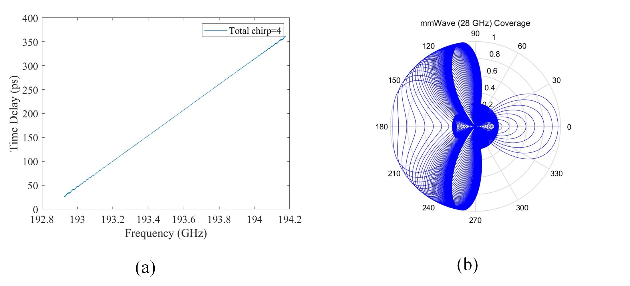
In this section, we present our novel beamforming design, where we obtain a relation between the optical signal after the CFBG1 and CFBG2 in the CU of Fig. 4 and its time delay imposed in Fig. 5(a). Explicitly, as portrayed in Fig. 5 by tuning a supported beam’s deflection as detailed in [28], we are capable of changing the total chirp, resulting in a linear relation between time-delay and the optical frequency as depicted in Fig. 5(a), hence resulting in a multi-service beam coverage around 180^∘ as shown in Fig. 5(b).

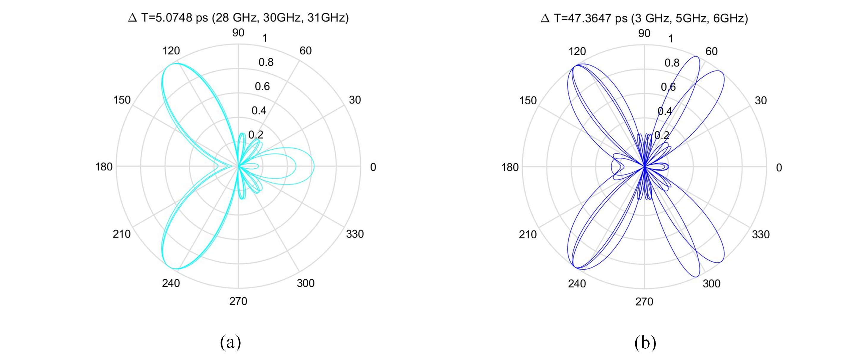
Moreover, to prove that our design can provide the same directive beam for both sub-6GHz and mmWave spectrum, as analysed in Section III, the CFBG1 and CFBG2 of Fig. 3 are required to impose the same degree of time-delay difference, while CFBG 3 is tuned to a time-delay related to the CFBG 1 and CFBG 2. As shown in Fig 6, the sub-6GHz beams are directed to the same direction at $\Delta T_{1}=47.3647$ to the mmWave beam at $\Delta T_{2}=5.0748$ , where the relation happens to be $\Delta T_{1}=d_{2}*\Delta T_{2}/d_{1}$ ⁶⁶6In our example, $d_{1}=\lambda_{3GHz}/2$ and $d_{2}=\lambda_{28GHz}/2$ are the inter-element distances of the sub-6GHz antenna array and mmWave antenna array, respectively, where we assume the center frequencies are 3 GHz and 28 GHz. Then we have $d_{2}/d_{1}=0.107$ ..

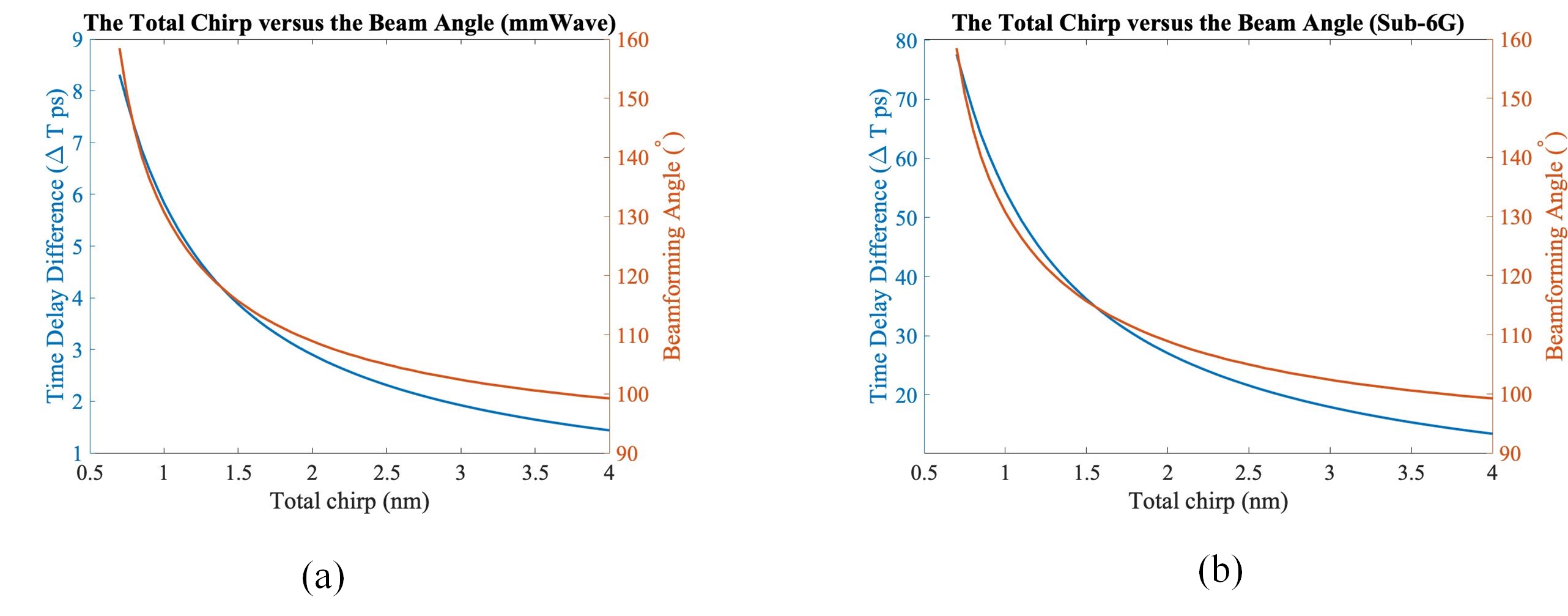
Explicitly, it is shown in Fig. 7(a) and 7(b) that the sub-6GHz and mmWave band are capable of being mapped to the same beamforming angle, thanks to the introduction of CFBG 3 in the RRH of Fig. 3. When the total chirp of both the CFBG 1 and CFBG 2 ranges from 0.7 to 4 nm with a step-size of 0.05, the time delay difference of sub-6GHz and mmWave spans from 77.6 ps to 13.4 ps and from 8.3 to 1.4 ps, respectively, which results in a beam angle from 158.48 to 99.23 ^∘ as shown in Fig. 7(a) and 7(b). Thus, by controlling the total chirp of the CFBG 3 in the RRH according to the total chirp in the CU, we can direct the multi-service to the same direction as shown in Fig. 6.

Then, as shown in Fig. 6(b) and Fig. 5, the corresponding multi-service beam coverage, which is around 180^∘ with a high precision, verifies that our photonic beamforming system can radiate the wideband beam flexibly and widely, while substantially simplifying the RRH designs as analysed in Section III.

V Conclusion

In this article, we have proposed a low-cost A-RoF aided multi-service communications in the two-hop relay train system, where we implemented the photonic beamformer using the CFBGs, enabling a centralised and low-cost RAN design. In this paper, we designed a double time-delay mapping rule of the optical signals and the corresponding RF signals and verified that the proposed system was capable of reducing the total cost of the RAN by simplifying the RRHs. Finally, a single beam transmitting the multi-service signals with a 180^∘ beamfroming range was presented.

References

[1] J. Kim, M. Schmieder, M. Peter, H. Chung, S. Choi, I. Kim, and Y. Han, “A comprehensive study on mmWave-based mobile hotspot network system for high-speed train communications,” IEEE Transactions on Vehicular Technology, vol. 68, no. 3, pp. 2087–2101, 2019.
[2] B. L. Dang, M. G. Larrode, R. V. Prasad, I. Niemegeers, and A. Koonen, “Radio-over-fiber based architecture for seamless wireless indoor communication in the 60 GHz band,” Computer communications, vol. 30, no. 18, pp. 3598–3613, 2007.
[3] A. Osseiran, J. F. Monserrat, and P. Marsch, 5G mobile and wireless communications technology. Cambridge University Press, 2016.
[4] A. Kanno, P. T. Dat, N. Yamamoto, T. Kawanishi, N. Iwasawa, N. Iwaki, K. Nakamura, K. Kawasaki, N. Kanada, N. Yonemoto, Y. Sato, M. Fujii, K. Yanatori, N. Shibagaki, and K. Kashima, “High-speed railway communication system using linear-cell-based radio-over-fiber network and its field trial in 90-ghz bands,” Journal of Lightwave Technology, vol. 38, no. 1, pp. 112–122, 2020.
[5] J. D. Oliva SÃ¡nchez and J. I. Alonso, “A two-hop MIMO relay architecture using LTE and millimeter wave bands in high-speed trains,” IEEE Transactions on Vehicular Technology, vol. 68, no. 3, pp. 2052–2065, 2019.
[6] Y. Li, M. El-Hajjar, and L. Hanzo, “Joint space-time block-coding and beamforming for the multi-user radio over plastic fiber downlink,” IEEE Transactions on Vehicular Technology, vol. PP, no. 99, pp. 1–1, 2017.
[7] A. Goldsmith, Wireless communications. Cambridge university press, 2005.
[8] L. Hanzo, H. Haas, S. Imre, D. O’Brien, M. Rupp, and L. Gyongyosi, “Wireless myths, realities, and futures: From 3G/4G to optical and quantum wireles,” Proceedings of the IEEE.
[9] P. T. Dat, A. Kanno, N. Yamamoto, and T. Kawanishi, “WDM RoF-MMW and linearly located distributed antenna system for future high-speed railway communications,” IEEE Communications Magazine, vol. 53, no. 10, pp. 86–94, 2015.
[10] I. A. Hemadeh, K. Satyanarayana, M. El-Hajjar, and L. Hanzo, “Millimeter-wave communications: Physical channel models, design considerations, antenna constructions, and link-budget,” IEEE Communications Surveys Tutorials, vol. 20, no. 2, pp. 870–913, 2018.
[11] A. Checko, H. L. Christiansen, Y. Yan, L. Scolari, G. Kardaras, M. S. Berger, and L. Dittmann, “Cloud RAN for mobile networks—–a technology overview,” IEEE Communications Surveys Tutorials, vol. 17, pp. 405–426, First quarter 2015.
[12] A. Alkhateeb, J. Mo, N. Gonzalez-Prelcic, and R. W. Heath, “MIMO precoding and combining solutions for millimeter-wave systems,” IEEE Communications Magazine, vol. 52, no. 12, pp. 122–131, 2014.
[13] V. A. Thomas, M. El-Hajjar, and L. Hanzo, “Millimeter-wave radio over fiber optical upconversion techniques relying on link nonlinearity,” IEEE Communications Surveys Tutorials, vol. 18, pp. 29–53, Firstquarter 2016.
[14] Y. Li, F. Wang, M. El-Hajjar, and L. Hanzo, “Analog radio-over-fiber-aided optical-domain MIMO signal processing for high-performance low-cost radio access networks,” IEEE Communications Magazine, vol. 59, no. 1, pp. 126–132, 2021.
[15] Z. Cao, Q. Ma, A. B. Smolders, Y. Jiao, M. J. Wale, C. W. Oh, H. Wu, and A. M. J. Koonen, “Advanced integration techniques on broadband millimeter-wave beam steering for 5G wireless networks and beyond,” IEEE Journal of Quantum Electronics, vol. 52, no. 1, pp. 1–20, 2016.
[16] Y. Li, Q. Yang, I. A. Hemadeh, M. El-Hajjar, C.-K. Chan, and L. Hanzo, “Experimental characterization of the radio over fiber aided twin-antenna spatial modulation downlink,” Opt. Express, vol. 26, pp. 12432–12440, May 2018.
[17] Y. Li, I. A. Hemadeh, M. El-Hajjar, and L. Hanzo, “Radio over fiber downlink design for spatial modulation and multi-set space-time shift-keying,” IEEE Access, vol. PP, no. 99, pp. 1–1, 2018.
[18] V. Thomas, M. El-Hajjar, and L. Hanzo, “Performance improvement and cost reduction techniques for radio over fiber communications,” IEEE Communications Surveys Tutorials, vol. 17, pp. 627–670, Second quarter 2015.
[19] Y. Li, S. Ghafoor, K. Satyanarayana, M. El-Hajjar, and L. Hanzo, “Analogue wireless beamforming exploiting the fiber-nonlinearity of radio over fiber-based c-rans,” IEEE Transactions on Vehicular Technology, vol. 68, no. 3, pp. 2802–2813, 2019.
[20] G. Vasileiou, G. I. Papadimitriou, P. Nicopolitidis, and P. G. Sarigiannidis, “An effective resource allocation medium access control protocol for radio-over-fiber access networks based on wavelength reuse,” Computer Communications, vol. 88, pp. 45–56, 2016.
[21] A. Molony, L. Zhang, J. Willlams, I. Bennion, C. Edge, and J. Fells, “Fiber Bragg grating networks for time-delay control of phased-array antennas,” in Lasers and Electro-Optics, 1996. CLEO’96., Summaries of papers presented at the Conference on, pp. 244–245, IEEE, 1996.
[22] G. A. Ball, W. Glenn, and W. Morey, “Programmable fiber optic delay line,” IEEE photonics technology letters, vol. 6, pp. 741–743, 1994.
[23] D. B. Hunter, M. E. Parker, and J. L. Dexter, “Demonstration of a continuously variable true-time delay beamformer using a multichannel chirped fiber grating,” IEEE Transaction on Microwave Theory and Techniquess on, vol. 54, no. 2, pp. 861–867, 2006.
[24] J. Yao, J. Yang, and Y. Liu, “Continuous true-time-delay beamforming employing a multiwavelength tunable fiber laser source,” IEEE Photonics Technology Letters, vol. 14, no. 5, pp. 687–689, 2002.
[25] J. Wang, H. Zhu, and N. J. Gomes, “Distributed antenna systems for mobile communications in high speed trains,” IEEE Journal on Selected Areas in Communications, vol. 30, no. 4, pp. 675–683, 2012.
[26] G. Liu, Y. Huang, Z. Chen, L. Liu, Q. Wang, and N. Li, “5G deployment: Standalone vs. non-standalone from the operator perspective,” IEEE Communications Magazine, vol. 58, no. 11, pp. 83–89, 2020.
[27] T. Han and N. Ansari, “Radiate: radio over fiber as an antenna extender for high-speed train communications,” IEEE Wireless Communications, vol. 22, no. 1, pp. 130–137, 2015.
[28] Yunqi Liu, Jianliang Yang, and Jianping Yao, “Continuous true-time-delay beamforming for phased array antenna using a tunable chirped fiber grating delay line,” IEEE Photonics Technology Letters, vol. 14, no. 8, pp. 1172–1174, 2002.
[29] F. Ellinger, U. Mayer, M. Wickert, N. Joram, J. Wagner, R. Eickhoff, I. Santamaria, C. Scheytt, and R. Kraemer, “Integrated adjustable phase shifters,” IEEE Microwave Magazine, vol. 11, no. 6, pp. 97–108, 2010.
[30] M. Cai, K. Gao, D. Nie, B. Hochwald, J. N. Laneman, H. Huang, and K. Liu, “Effect of wideband beam squint on codebook design in phased-array wireless systems,” in 2016 IEEE Global Communications Conference (GLOBECOM), pp. 1–6, 2016.
[31] B. Wang, M. Jian, F. Gao, G. Y. Li, and H. Lin, “Beam squint and channel estimation for wideband mmwave massive MIMO-OFDM systems,” IEEE Transactions on Signal Processing, vol. 67, no. 23, pp. 5893–5908, 2019.