Temporal Context Mining for Learned Video Compression

Abstract

Applying deep learning to video compression has attracted increasing attention in recent few years. In this work, we address end-to-end learned video compression with a special focus on better learning and utilizing temporal contexts. We propose to propagate not only the last reconstructed frame but also the feature before obtaining the reconstructed frame for temporal context mining. From the propagated feature, we learn multi-scale temporal contexts and re-fill the learned temporal contexts into the modules of our compression scheme, including the contextual encoder-decoder, the frame generator, and the temporal context encoder. We discard the parallelization-unfriendly auto-regressive entropy model to pursue a more practical encoding and decoding time. Experimental results show that our proposed scheme achieves a higher compression ratio than the existing learned video codecs. Our scheme also outperforms x264 and x265 (representing industrial software for H.264 and H.265, respectively) as well as the official reference software for H.264, H.265, and H.266 (JM, HM, and VTM, respectively). Specifically, when intra period is 32 and oriented to PSNR, our scheme outperforms H.265–HM by 14.4% bit rate saving; when oriented to MS-SSIM, our scheme outperforms H.266–VTM by 21.1% bit rate saving.

I Introduction

Video data contributes to most of the internet traffic nowadays. Therefore, efficient video compression is always a high demand to reduce the transmission and storage cost. In the past two decades, several video coding standards have been developed, including H.264/AVC [1], H.265/HEVC [2], and H.266/VVC [3].

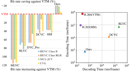
Figure 1: Compression ratio in terms of MS-SSIM when intra period is 32 and running time on 1080p videos. As traditional video codecs are optimized for CPU, we report their run time on CPU, which is the same as previous schemes[4, 5]. The learned video codecs are run on GPU.

Recently, learned video compression has explored a new direction. Existing learned video compression can be roughly categorized into four classes. Residual coding-based schemes [6, 5, 7, 8, 4, 9, 10, 11, 12, 13, 14, 15, 16, 17, 18, 19, 20, 21, 22]: prediction is first applied in the pixel domain or feature domain. Then the residue from the prediction is compressed. Volume coding-based schemes [23, 24, 25]: videos are regarded as volumes containing multiple frames. 3D convolutions are applied to get the latent representations. Entropy coding-based schemes [26]: each frame is encoded with independent image codec. The correlations between the latent representations in different frames are explored to guide the entropy modeling. Conditional coding-based schemes [27]: temporal contexts are served as conditions and the temporal correlation is explored by the encoder automatically. There are also some other schemes focusing on the perceptual quality optimization for learned codecs [28, 29]. We agree that perceptual quality is more important and learned codecs have benefits on optimizing for perceptual quality over traditional codecs due to the end-to-end training and back-propagation. However, this paper still focuses on objective distortion metrics to make the comparison with previous schemes easier.

Among the existing learned video codecs, Li et al. proposed a deep contextual video compression (DCVC) framework and achieved the state-of-the-art compression ratio [27]. DCVC is an open framework based on the aforementioned conditional coding structure. DCVC generates a single-scale temporal context from the previously decoded frame with motion compensation and several convolutional layers. It is a simple yet useful method. However, the previously decoded frame loses much texture and motion information as it only contains three channels. Moreover, a single-scale context may not contain sufficient temporal information. Therefore, in this paper, we try to find a better way to learn and utilize temporal contexts.

Following the conditional coding structure, we propose a temporal context mining (TCM) module to learn richer and more accurate temporal contexts. We propagate the feature before obtaining the reconstructed frame and learn temporal contexts from the propagated features for the current frame using the TCM module. Considering that learning a single-scale context may not describe the spatio-temporal non-uniformity well [30, 31, 32], the TCM module adopts a hierarchical structure to generate multi-scale temporal contexts. Finally, we re-fill the learned temporal contexts into the modules of our compression scheme, including the contextual encoder-decoder, the frame generator, and the temporal context encoder. We refer to the procedure as temporal context re-filling (TCR).

Following most previous schemes, this paper focuses on the scenarios with delay constraint or called low-delay coding although random-access is the most efficient coding configuration. Some schemes reported higher compression ratios than H.265/HEVC, but most of them just used x265 [33], which is optimized for fast encoding time and cannot represent the best compression ratio of H.265/HEVC. In this paper, we try our best to compare with the best traditional video codecs. We use the official reference software JM [34], HM [35], and VTM [36] for H.264/AVC, H.265/HEVC, and H.266/VVC to represent the highest potential compression ratio, without playing any tricks to harm it. More details could be found in Sec. II-C. In addition, many schemes [17, 4, 23, 27, 37] used the auto-regressive entropy model [38] for a higher compression ratio, which poses significant challenges for parallel implementation and meanwhile greatly increases the decoding time. We do not apply the auto-regressive entropy model in any part of our scheme to build a parallelization-friendly decoder, although we agree that the auto-regressive entropy model could further boost the compression ratio by a large margin. Fig. 1 compares the compression ratio and running time on 1080p videos. Our scheme achieves much faster encoding and decoding speed than the other learned video codecs. To the best of our knowledge, this is the first end-to-end learned video compression scheme achieving such a milestone result that outperforms HM in terms of peak signal-to-noise ratio (PSNR) and VTM in terms of multi-scale structural similarity index measure (MS-SSIM) [39].

Our contributions are summarized as follows:

• We propose a temporal context mining module to learn multi-scale temporal contexts from the propagated features rather than the previously reconstructed frames.

• We propose to re-fill the learned multi-scale temporal contexts into the contextual encoder-decoder, the frame generator, and the temporal context encoder to help compress and reconstruct the current frame.

• Without the auto-regressive entropy model, our proposed scheme achieves higher compression ratio than the existing learned video codecs. Our scheme also outperforms the reference software of H.265/HEVC—HM by 14.4% in terms of PSNR and outperforms the reference software of H.266/VVC—VTM by 21.1% in terms of MS-SSIM. We will release code to facilitate the future investigation.

The remainder of this paper is organized as follows. Section II gives a brief review of related work. Section III describes the methodology of our proposed scheme. Section IV presents the experimental results and analysis of the proposed scheme. Section V concludes this paper and discuss the future investigate.

II Related Work

II-A Traditional Video Compression

Traditional video compression has been developed for several decades, and several video coding standards have been proposed. H.264/AVC [2] was initially developed in the period between 1999 and 2003 by the well-known ITU-T and ISO/IEC standards. It achieves great success and is widely used for many applications, such as broadcast of high-definition TV signals and internet and mobile network video. Along with the increase of video resolution and use of parallel processing architectures, H.265/HEVC [1] was finalized in 2013 and offered about 50% bit rate saving over H.264/AVC. The superior compression efficiency of H.265/HEVC enables the popularity of 4K video with increased fidelity. H.266/VVC [3] is the new generation of international video coding standard. It is designed not only to reduce a substantial bit rate compared to H.265/HEVC, but also to cover all current and emerging media needs. These video coding standards follow a similar hybrid video coding framework, including prediction, transform, quantization, entropy coding, and loop filtering. Although the learned image codecs [40, 41] have caught up with or even surpassed the traditional image coding schemes, the traditional video compression scheme is still state-of-the-art in terms of compression ratio.

II-B Learned Video Compression

Learned video compression has explored a new direction in recent years. Lu et al. replaced each part in the traditional motion-compensated prediction and residual coding framework with convolutional neural networks [4]. They jointly optimized the whole network with the rate-distortion cost. Lin et al. explored multiple reference frames and associated multiple motion vectors to generate a more accurate prediction of the current frame and reduce the coding cost of motion vectors [9]. Yang et al. designed a recurrent learned video compression scheme [16]. The proposed recurrent auto-encoder and recurrent probability model use the temporal information in a large range of frames to generate latent representations and reconstruct compressed output. Hu et al. extracted the features of the input frames and applied deformable convolution to perform motion prediction [10]. The learned offset and residue are compressed in the feature domain. Then multiple reference features stored in the decoded buffer are fused by a non-local attention module to obtain the reconstructed frame. Except for the motion-compensated prediction and residual coding framework, Habibian et al. regarded the video as a volume of multiple frames and proposed a 3D auto-encoder to directly compress multiple frames [23]. Liu et al. used the image codec to compress each frame and proposed an entropy model to explore the temporal correlation of the latent representations [26]. Li et al. shifted the paradigm from residual coding to conditional coding [27]. They learned temporal contexts from the previously decoded frame and let the encoder explore the temporal correlation to remove the redundancy automatically.

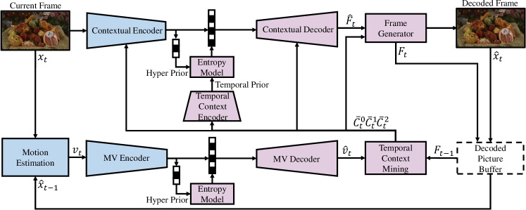
Figure 2: Overview of our proposed video compression scheme. Given an input frame $x_{t}$, the motion vector (MV) between $x_{t}$ and previously decoded frame $\hat{x}_{t-1}$ is estimated, compressed, and then reconstructed. A temporal context mining (TCM) module is proposed to learn multi-scale temporal contexts from the propagated feature $F_{t-1}$ instead of the previously decoded frame $\hat{x}_{t-1}$. The temporal contexts ($\bar{C}_{t}^{0},\bar{C}_{t}^{1},\bar{C}_{t}^{2}$) are re-filled into the contextual encoder-decoder, the frame generator, and the temporal context encoder to compress and reconstruct the current frame $x_{t}$. The decoded frame $\hat{x}_{t}$ and the feature $F_{t}$ before obtaining $\hat{x}_{t}$ are propagated to help compress the next frame $x_{t+1}$. The blue modules are only used at the encoder side. The lavender modules are used at both the encoder and the decoder sides.

II-C Traditional Video Codecs versus Learned Video Codecs

Although many existing learned video codecs reported a better compression ratio than H.265/HEVC, they may not use the best encoder with the following major issues. Firstly, x264 [42] and x265 [33] are used to represent the compression ratio of H.264/AVC and H.265/HEVC, respectively. However, they are optimized for faster encoding instead of a higher compression ratio. The official reference software JM [34], HM [35], and VTM [36] should be used to represent the higher compression ratio. For example, the gap between x265 and HM is about 80%, as shown in Table I. Secondly, an unrealistic intra period of 10 or 12 is used to limit temporal error propagation [43]. However, in real applications, the bits of I frames account for a substantial part of the total number of bits when using such a small intra period. Taking the VTM as an example, the bits of I frame account for 51% for intra period 12 and account for 29% for intra period 32. Intra period 12 is harmful to the compression ratio and is seldom used in the real world. Therefore, this paper proposes to use intra period 32 (roughly 1 second for 30fps), which is more reasonable to measure the performance of inter coding for video codecs. Thirdly, the internal color space of YUV420 is set for traditional codecs in existing schemes. However, after comparing different color spaces for traditional codecs, we conclude that YUV444 is better than YUV420 and RGB, even though the final distortion is measured in RGB. The performance gap is more than 30%. Thus, we propose to use YUV444 as the internal color space for JM, HM, and VTM in favor of seeking the higher potential compression ratio of the traditional codecs. A similar conclusion has been made in learned image compression [40]. Fourthly, we use the best suitable configuration (e.g., using range extension profile to encode YUV444 content) for traditional codecs as the performance gap of different configurations can be over 40%.

III Methodology

III-A Overview

Aiming to find a better way to learn and utilize temporal contexts, we propose a new learned video compression scheme based on temporal context mining and re-filling. An overview of our scheme is depicted in Fig. 2.

III-A1 Motion Estimation

We feed the current frame $x_{t}$ and the previously decoded frame $\hat{x}_{t-1}$ into a neural network-based motion estimation module to estimate the optical flow. The optical flow is considered as the estimated motion vector (MV) $v_{t}$ for each pixel. In this paper, the motion estimation module is based on the pre-trained Spynet [44].

III-A2 MV Encoder-Decoder

After obtaining the motion vectors $v_{t}$, we use the MV encoder and decoder to compress and reconstruct the input MV $v_{t}$ in a lossy way. Specifically, $v_{t}$ is compressed by an auto-encoder with the hyper prior structure [45]. The reconstructed MV is denoted as $\hat{v}_{t}$.

III-A3 Learned Temporal Contexts

We propose a TCM module to learn richer and more accurate temporal contexts from the propagated feature $F_{t-1}$ instead of the previously decoded frame $\hat{x}_{t-1}$. Instead of producing only a single-scale temporal context, the TCM module generates multi-scale temporal contexts $\bar{C_{t}}^{l}$ to capture spatial-temporal non-uniform motion and texture, where $l$ is the index of different scales. The learned temporal contexts are re-filled in the contextual encoder-decoder, the frame generator, and the temporal context encoder to help improve the compression ratio. This procedure is referred to as TCR. We will introduce them in detail in Section III-B and III-C.

III-A4 Contextual Encoder-Decoder and Frame Generator

With the assistance of the re-filled multi-scale temporal contexts $\bar{C_{t}}^{l}$, the contextual encoder-decoder and the frame generator are used to compress and reconstruct the current frame $x_{t}$. We denote the decoded frame as $\hat{x}_{t}$ and the feature before obtaining $\hat{x}_{t}$ as $F_{t}$. $\hat{x}_{t}$ and $F_{t}$ are propagated to help compress the next frame $x_{t+1}$. The details are presented in Section III-C.

III-A5 Temporal Context Encoder

To utilize the temporal correlation of the latent representations of different frames produced by the contextual encoder, we use a temporal context encoder to generate the temporal prior by taking advantage of the multi-scale temporal contexts $\bar{C_{t}}^{l}$. More information is provided in Section III-C.

III-A6 Entropy Model

We use the factorized entropy model for hyper prior and Laplace distribution to model the latent representations as [27]. We do not apply the auto-regressive entropy model to make the decoding processes parallelization-friendly, even though it is helpful to improve the compression ratio. For the contextual encoder-decoder, we fuse the hyper and temporal priors [27] to estimate more accurate parameters of Laplace distribution. When writing bitstream, we apply a similar implementation as in [46].

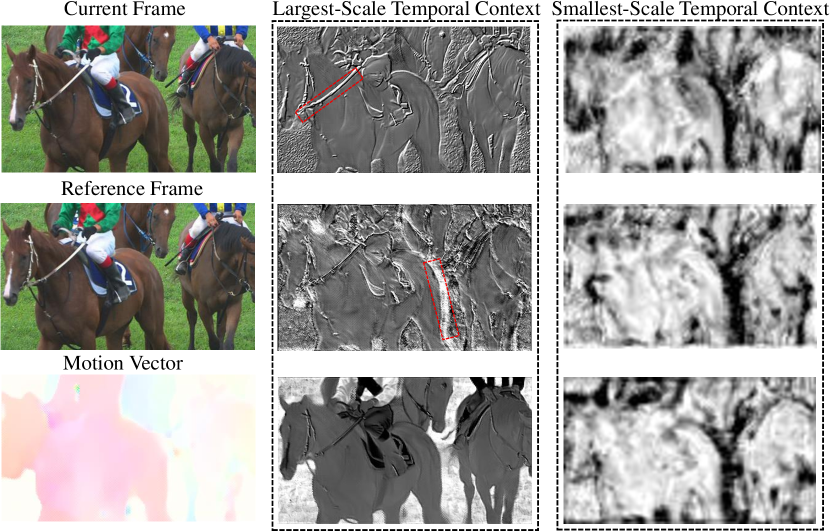
Figure 3: Visualization of the multi-scale temporal contexts. In the largest-scale context, some channels focus on the texture information and some focus on the color information. In the smallest-scale context, channels mainly focus on the regions with large motion.

III-B Temporal Context Mining

Considering that the previously decoded frame $\hat{x}_{t-1}$ loses much information as it only contains three channels, it is not optimal to learn temporal contexts from $\hat{x}_{t-1}$. In our paper, we propose a TCM module to learn temporal contexts from the propagated feature $F_{t-1}$. Different from the existing video compression schemes in feature domain [10, 47, 11], which extract features from the previously decoded frame $\hat{x}_{t-1}$, we propagate the feature $F_{t-1}$ before obtaining $\hat{x}_{t-1}$. Specifically, in the reconstruction procedure of $\hat{x}_{t-1}$, we store the feature $F_{t-1}$ before the last convolutional layer of the frame generator in the generalized decoded picture buffer (DPB). To reduce the computational complexity, instead of storing multiple features of previously decoded frames [10, 11], we only store a single feature. Then $F_{t-1}$ is propagated to learn temporal contexts for compressing the current frame $\hat{x}_{t}$. For the first P frame, we still extract the feature from the reconstructed I frame, to make the model adapt to different image codecs.

Besides, learning a single scale context may not describe the spatio-temporal non-uniform motion and texture well [30, 31, 32]. As shown in Fig. 3, in the largest-scale context, some channels focus on the texture information and some focus on the color information. In the smallest-scale context, channels mainly focus on the regions with large motion. Therefore, a hierarchical approach is performed to learn multi-scale temporal contexts.

As shown in Fig. 4, we first generate multi-scale features $F_{t-1}^{l}$ from the propagated feature $F_{t-1}$ using a feature extraction module ($extract$) with $L$ levels which consists of convolutional layers and residual blocks [48] (three levels are used in our paper).

$$F_{t-1}^{l}=extract\left(F_{t-1}\right),l=0,1,2$$ (1)

Meanwhile, the decoded MV $\hat{v}_{t}$ are downsampled using the bilinear filter to generate multi-scale MVs $\hat{v}_{t}^{l}$, where $\hat{v}_{t}^{0}$ is set to $\hat{v}_{t}$. Note that each downsampled MV is divided by 2. Then, we warp ($warp$) the multi-scale features ${F}_{t-1}^{l}$ using the associated MV $\hat{v}_{t}^{l}$ at the same scale.

$$\bar{F}_{t-1}^{l}=warp\left(F_{t-1}^{l},\hat{v}_{t}^{l}\right),l=0,1,2$$ (2)

After that, we use an upsample ($upsample$) module, consisting of one subpixel layer [49] and one residual block, to upsample $\bar{F}_{t-1}^{l+1}$. The upsampled feature is then concatenated ($concat$) with $\bar{F}_{t-1}^{l}$ at the same scale.

$$\tilde{F}_{t-1}^{l}=concat\left(\bar{F}_{t-1}^{l},upsample\left(\bar{F}_{t-1}^{l+1}\right)\right),l=0,1$$ (3)

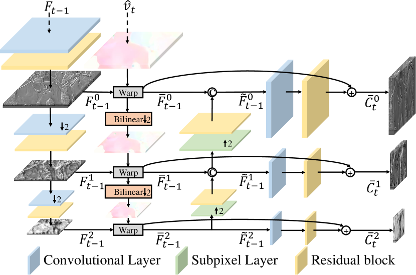
Figure 4: Architecture of the temporal context mining (TCM) module. The propagated feature $F_{t-1}$ is fed into the TCM module to generate multi-scale temporal contexts $\bar{C_{t}}^{l}$.

At each level of the hierarchical structure, a context refinement module $(refine)$, consisting of one convolutional layer and one residual block, is used to learn the residue [50]. The residue is added to $\bar{F}_{t-1}^{l}$ to generate the final temporal contexts $\bar{C}_{t}^{l}$, as illustrated in Fig 4.

$$\bar{C}_{t}^{l}=\bar{F}_{t-1}^{l}+refine\left(\tilde{F}_{t-1}^{l}\right),l=0,1,2$$ (4)

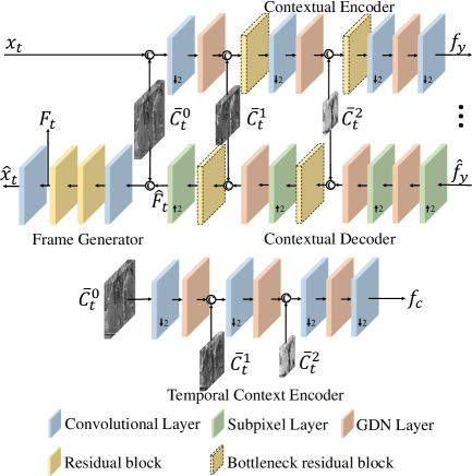
Figure 5: Illustration of temporal context re-filling (TCR). The multi-scale temporal contexts are re-filled into the contextual encoder-decoder, frame generator, and temporal context encoder.

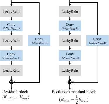
Figure 6: Architectures of residual block and bottleneck residual block. The numbers in a convolutional layer like ($3,N_{in},N_{mid},1$) refer to the kernel size is 3, the number of input channels is $N_{in}$, the number of output channels is $N_{mid}$, and the stride is 1.

III-C Temporal Context Re-filling

To fully take advantage of the temporal correlation, we re-fill the learned multi-scale temporal contexts into the modules of our compression scheme, including the contextual encoder-decoder, the frame generator, and the temporal context encoder, as shown in Fig. 5. The temporal context plays an important role in temporal prediction and temporal entropy modeling. With the re-filled multi-scale temporal contexts, the compression ratio of our scheme is improved a lot.

III-C1 Contextual Encoder-Decoder and Frame Generator

We concatenate the largest-scale temporal context $\bar{C}_{t}^{0}$ with the current frame $x_{t}$, and then feed them into the contextual encoder. In the process of mapping from $x_{t}$ to the latent representation $f_{y}$, we also concatenate $\bar{C}_{t}^{1}$ and $\bar{C}_{t}^{2}$ with other scales into the encoder. Symmetric with the encoder, the contextual decoder maps the quantized latent representation $\hat{f}_{y}$ to the feature $\hat{F}_{t}$ with the assistance of $\bar{C}_{t}^{1}$ and $\bar{C}_{t}^{2}$. Then $\hat{F}_{t}$ and $\bar{C}_{t}^{0}$ are concatenated and fed into the frame generator to obtain the reconstructed frame $\hat{x}_{t}$. Considering that the concatenation increases the number of channels, a “bottleneck” building residual block is used to reduce the complexity of the middle layer. The detailed architectures are illustrated in Fig. 6. The feature $F_{t}$ before the last convolutional layer of the frame generator is propagated to help compress the next frame $x_{t+1}$.

III-C2 Temporal Context Encoder

To explore the temporal correlation of the latent representations of different frames, we use a temporal context encoder to obtain the lower-dimensional temporal prior $f_{c}$. Instead of using a single-scale temporal context as [27], we concatenate the multi-scale temporal contexts in the process of generating temporal prior. The temporal prior is fused with the hyper prior to estimate the means and variance of Laplacian distribution for the latent representation $\hat{f}_{y}$. The architecture of the temporal context encoder is presented in Fig. 5.

III-D Loss Function

Our scheme targets to jointly optimize the rate-distortion (R-D) cost.

$$L_{t}=\lambda D_{t}+R_{t}=\lambda d(x_{t},\hat{x}_{t})+R_{t}^{\hat{v}}+R_{t}^{\hat{f}}$$ (5)

$L_{t}$ is the loss function for the current time step $t$. $d(x_{t},\hat{x}_{t})$ refers to the distortion between the input frame $x_{t}$ and the reconstructed frame $\hat{x}_{t}$, where $d(\cdot)$ denotes the mean-square-error or 1$-$MS-SSIM [39]. $R_{t}^{\hat{v}}$ represents the bit rate used for encoding the quantized motion vector latent representation and the associated hyper prior. $R_{t}^{\hat{f}}$ represents the bit rate used for encoding the quantized contextual latent representation and the associated hyper prior. We train our model step-by-step to make the training more stable as previous the scheme[9]. It is worth mentioning that, in the last five epochs, we use a commonly-used training strategy in recent papers [8, 16, 43, 51], that trains our model on the sequential training frames to alleviate the error propagation.

$$L^{T}=\frac{1}{T}\sum_{t}L_{t}=\frac{1}{T}\sum_{t}\left\{\lambda d\left(x_{t},\hat{x}_{t}\right)+R_{t}^{\hat{v}}+R_{t}^{\hat{f}}\right\}$$ (6)

where $T$ is the time interval and set as 4 in our experiments.

IV Experiments

IV-A Experimental Setup

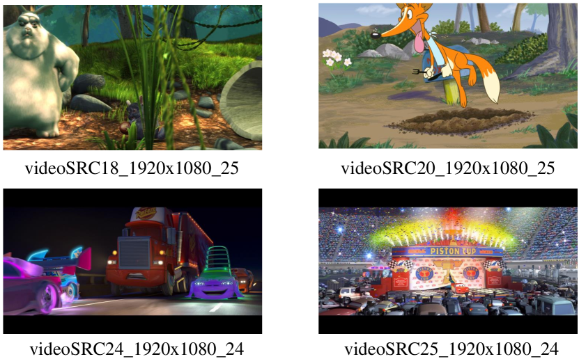
Figure 7: Visualization of the four animations sequences (18, 20, 24, 25) which are excluded by the MCL-JCV-26 dataset.

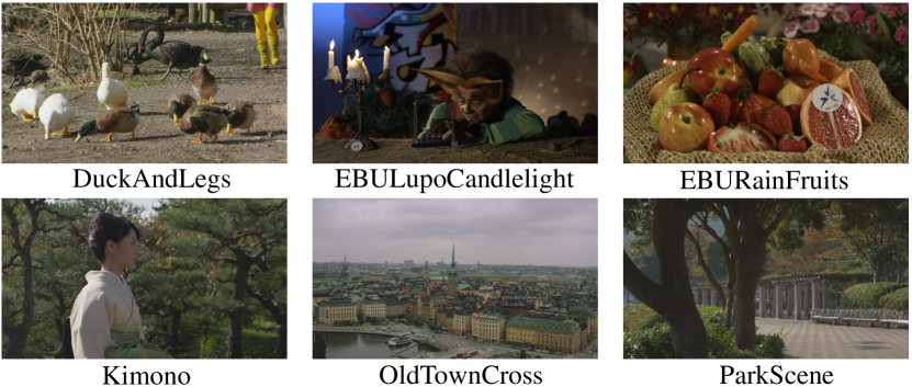
Figure 8: HEVC Class RGB consists of 6 1080p video sequences with 10 bit depth and in RGB444 format defined in the common test conditions for HEVC range extensions [52], including DucksAndLegs, EBULupoCandlelight, DucksAndLegs, DucksAndLegs, Kimono, OldTownCross, and ParkScene.

IV-A1 Datasets

Many training datasets are produced for learned video compression [53, 54, 55]. Following most previous schemes[9, 4, 16, 27], in our work, we use the commonly-used Vimeo-90k [55] training split, and randomly crop the videos into $256\times 256$ patches. To evaluate the performance and application domain of our proposed video compression scheme, we use UVG [56], MCL-JCV [57], and HEVC datasets [2]. These datasets contain various video contents, including slow/fast motion and poor/high quality, which are commonly used in leaned video compression. The UVG dataset has 7 1080p sequences and the MCL-JCV dataset has 30 1080p sequences. Considering the animations sequences in MCL-JCV (18, 20, 24, 25) are quite different from the natural videos in the training dataset, as shown in Fig. 7, we follow the setting in [12] and build another MCL-JCV-26 dataset which excludes the four animations sequences. The HEVC dataset contains 16 sequences including Class B, C, D, and E. The source videos of these datasets are in YUV420 format while PSNR is calculated in RGB color space. Therefore, we build an additional class called HEVC Class RGB, which includes add 6 1080p videos with 10 bit depth and in RGB444 format defined in the common test conditions for HEVC range extensions [52]: DucksAndLegs, EBULupoCandlelight, DucksAndLegs, DucksAndLegs, Kimono, OldTownCross, and ParkScene, as illustrated in Fig. 8.

IV-A2 Implementation Details

We train four models with different $\lambda$ values ($\lambda=256,512,1024,2048$) for multiple coding rates. The AdamW [58] optimizer is used and the batch size is set to 4. When using MS-SSIM for performance evaluation, we fine-tune the model by using 1$-$MS-SSIM as the distortion loss with different $\lambda$ values ($\lambda=8,16,32,64$). Our model is implemented with PyTorch and trained on 2 NVIDIA V100 GPUs. It takes 2.5 days to train our model.

IV-A3 Evaluation Metrics

We use bpp (bit per pixel) to measure the bits cost for one pixel in each frame. We use PSNR and MS-SSIM to evaluate the distortion between the decoded frame and the original frame.

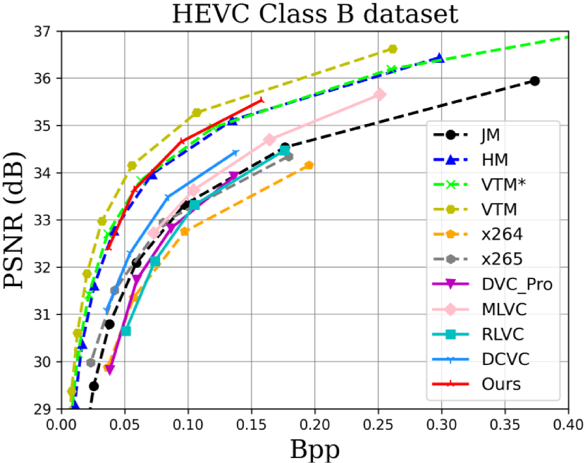
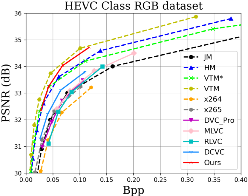
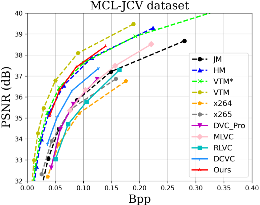
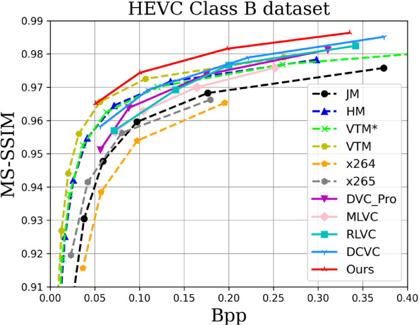
Figure 9: Rate-distortion performance of our proposed scheme on the HEVC Class B, HEVC Class RGB and MCL-JCV datasets. Intra period is set to 32.

TABLE I: BD-rate for PSNR (intra period 32). The anchor is HM.

	HM	JM	VTM	VTM*	x264	x265	DVC_Pro	MLVC	RLVC	DCVC	Ours
UVG	0.0	108.1	–28.9	4.6	176.8	109.2	137.7	66.5	140.1	67.3	–9.0
MCL-JCV	0.0	95.4	–31.2	–7.2	143.3	84.4	99.3	66.8	124.8	42.8	–3.2
MCL-JCV-26	0.0	101.9	–31.0	–6.4	161.0	93.6	92.0	56.1	115.8	37.3	–9.7
HEVC Class B	0.0	96.9	–28.8	–8.2	144.6	76.1	123.7	61.4	122.6	56.0	–5.3
HEVC Class C	0.0	56.6	–29.0	–3.8	79.8	46.2	124.0	124.1	118.9	76.9	15.1
HEVC Class D	0.0	50.0	–26.5	–3.5	72.0	43.8	93.6	96.1	81.2	52.8	–5.4
HEVC Class E	0.0	80.5	–29.1	–10.0	153.2	60.3	283.0	138.8	246.2	156.8	18.5
HEVC Class RGB	0.0	102.4	–29.7	–1.7	151.9	82.8	102.1	82.1	114.2	51.9	–14.4

• †Unless otherwise specified, we configure JM, HM, and VTM with the highest-compression-ratio settings for low-delay coding.

• ‡VTM* uses one reference frame instead of the default four frames in VTM. Note that our scheme uses one reference frame for motion estimation.

TABLE II: BD-rate for MS-SSIM (intra period 32). The anchor is HM.

	HM	JM	VTM	VTM*	x264	x265	DVC_Pro	MLVC	RLVC	DCVC	Ours
UVG	0.0	105.6	–27.0	2.3	169.9	87.9	36.2	64.7	49.4	9.2	–25.5
MCL-JCV	0.0	108.5	–30.4	–5.8	141.0	71.9	7.8	50.3	34.5	–16.3	–38.3
MCL-JCV-26	0.0	113.4	–30.3	–6.5	152.0	74.3	0.7	44.2	23.3	–18.8	–40.5
HEVC Class B	0.0	112.4	–26.9	–4.2	150.3	71.1	23.5	50.2	28.3	0.9	–40.8
HEVC Class C	0.0	61.3	–27.9	–3.4	89.9	53.5	17.0	53.1	30.0	–8.9	–42.4
HEVC Class D	0.0	52.4	–25.9	–3.0	80.0	49.7	–7.8	40.4	0.2	–24.2	–52.6
HEVC Class E	0.0	90.9	–27.8	–7.8	184.5	55.0	110.1	106.1	87.1	38.0	–40.9
HEVC Class RGB	0.0	107.4	–27.2	–3.9	135.9	64.9	18.3	51.8	21.5	3.3	–43.4

Figure 10: Rate-distortion performance of our proposed scheme on the HEVC Class B, HEVC Class RGB and MCL-JCV datasets. Intra period is set to 12.

TABLE III: BD-rate for PSNR (intra period 12). The anchor is HM.

	HM	JM	VTM*	x264	x265	DVC_Pro	MLVC	RLVC	DCVC	Ours
UVG	0.0	79.8	–7.6	139.2	77.7	43.5	37.8	63.2	13.8	–21.0
MCL-JCV	0.0	80.0	–13.3	124.4	67.8	38.7	46.4	73.6	10.0	–12.5
MCL-JCV-26	0.0	84.5	–12.9	138.8	74.8	32.9	37.1	65.1	4.4	–18.8
HEVC Class B	0.0	75.8	–16.8	113.3	53.7	36.9	34.6	54.0	9.5	–15.2
HEVC Class C	0.0	46.0	–11.7	62.7	31.3	46.3	78.1	58.9	26.1	4.7
HEVC Class D	0.0	40.9	–10.4	56.3	29.3	30.9	61.1	35.4	12.7	–10.2
HEVC Class E	0.0	62.7	–18.3	113.8	39.3	79.2	54.7	60.4	33.8	–6.4
HEVC Class RGB	0.0	78.7	–11.7	118.8	60.2	24.2	42.4	38.7	2.2	–23.0

• †VTM with the highest-compression-ratio settings for low-delay coding is not tested here because it does not support intra period 12.

TABLE IV: BD-rate for MS-SSIM (intra period 12). The anchor is HM.

	HM	JM	VTM*	x264	x265	DVC_Pro	MLVC	RLVC	DCVC	Ours
UVG	0.0	79.9	–9.3	132.5	59.5	–2.9	39.4	16.0	–16.1	–35.0
MCL-JCV	0.0	91.4	–12.3	121.8	54.2	–17.0	33.6	10.5	–30.7	–44.4
MCL-JCV-26	0.0	94.7	–13.1	129.8	54.9	–21.3	28.5	1.6	–32.8	–46.5
HEVC Class B	0.0	90.2	–13.0	118.6	49.4	–14.7	27.0	–3.7	–24.2	–48.5
HEVC Class C	0.0	49.7	–11.9	70.6	36.7	–17.5	27.3	–4.4	–29.8	–47.2
HEVC Class D	0.0	41.8	–9.6	62.2	34.9	–31.4	21.2	–24.7	–39.7	–55.1
HEVC Class E	0.0	69.7	–14.5	138.1	34.6	5.0	38.8	–5.3	–19.5	–53.9
HEVC Class RGB	0.0	84.6	–12.8	103.4	43.5	–20.3	20.8	–11.2	–25.1	–51.4

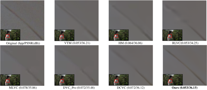
Figure 11: Subjective quality comparison on the 3rd frame of HEVC Class B Kimono sequence when the intra period is set to 32.

IV-B Experimental Results

IV-B1 Comparison Setting

Although random access is the most efficient coding mode, in this paper, we focus on low-delay coding mode following the setting of most previous schemes. Therefore, we set x264, x265, JM-19.0, HM-16.20, and VTM-13.2 under low-delay mode. For x264 and x265, we use the implementation in FFmpeg under veryslow preset. The internal color space is YUV420 as the previous schemes did. For JM, HM and VTM, we use the range extension profile instead of the main profile to enable the coding tools designed for non-YUV420. Specifically, we use encoder_JM_LB_HE, encoder_lowdelay_main_rext, encoder_lowdelay_vtm configuration, respectively. The internal color space is set to YUV444. Meanwhile, four reference frames are used for them as default for seeking the highest compression ratio. As analyzed in Section II-C, the bits of I frames account for a substantial part of the total number of bits. Therefore, for learned video codecs (DVC_Pro [4], MLVC [9], RLVC [16], DCVC [27]), we use the same image codec as our scheme to compress I frames to make a fair comparison. We adopt the Cheng2020Anchor [41] implemented by CompressAI [46] but we remove its auto-regressive entropy model [38]. The DVC_Pro models are trained by ourselves and the other models are released from the authors. In previous schemes, the intra period is set to 10 or 12 to limit temporal error propagation. However, such a small intra period is seldom used in real applications, as described in Section II-C. Therefore, we propose to use a more reasonable intra period of 32. To provide more information, we also test the cases of intra period 12. Since the GOP size of VTM with encoder_lowdelay_vtm configuration is 8, it does not support intra period 12. Therefore, we add a modified VTM* with low-delay P, 8-bit internal depth, and a single reference frame configuration. We encode 96 frames for each video in all testing datasets.

IV-B2 Results

Table I and Table II report the BD-rate [59] when the intra period is set to 32. Table III and Table IV report the BD-rate when the intra period is set to 12. The anchor is HM. Negative values indicate bit rate saving compared with HM while positive values indicate bit rate increasing. Experimental results show that, for intra period 32, our scheme outperforms HM by 14.4% and outperforms VTM* by 14.2% in terms of PSNR on HEVC Class RGB. Although our scheme still has a 25.4% PSNR performance gap compared with VTM with the best configuration, we outperform it by 21.1% in terms of MS-SSIM. For intra period 12, we achieve a larger compression ratio improvement. Note that, when comparing our scheme with VTM or VTM*, VTM or VTM* are regarded as the anchors and the BD-rate values are re-calculated instead of directly subtracting the values in the aforementioned tables. Compared with the results of intra period 32 and 12, our scheme still achieves a high comparison ratio while that of other learned video codecs is greatly reduced when using a larger intra period. Fig. 9 and Fig. 10 illustrate the RD-curves for different intra periods on HEVC Class B, HEVC Class RGB, and MCL-JCV. We find that learned video codecs behave better when the source videos are in RGB format. The subjective comparison results illustrated in Fig. 11 show that our scheme can retain more details.

TABLE V: Average encoding/decoding time for a 1080p frame (in seconds).

Schemes	Enc Time	Dec Time
VTM	743.88 s	0.31 s
HM	92.58 s	0.21 s
DCVC	12.26 s	35.59 s
RLVC	72.00 s	216.67 s
Ours	0.88 s	0.47 s

IV-B3 Model Complexity and Encoding/Decoding Time

The total number of parameters of our scheme is 10.7M. When processing one 1080p frame, the MACs (multiply–accumulate operation) of our scheme is 2.9T, while that of DCVC is 2.4T. Fig. 1 illustrates the average encoding and decoding time for one 1080p frame of different codecs. Table V lists the detailed values. Different from existing schemes which excluded the time for entropy coding [16, 27, 26] or data transfer between CPU and GPU [5], we include the time for model inference, entropy modeling, entropy decoding, and data transfer between CPU and GPU. Our encoding time refers to all the time from reading the original frame to writing bitstream into the hard disk and our decoding time refers to all the time from reading bitstream to generating the final reconstructed frame. As traditional video codecs are optimized for CPU, we run them on an Intel(R) Xeon(R) Platinum 8272CL CPU, which is the same with previous schemes[4, 5]. For learned video codecs, we run them on a NVIDIA V100 GPU. We only compare with the learned video codecs whose officially released codes enable bitstream writing. The comparison shows that our scheme takes 0.88s to encode a 1080p frame and takes 0.47s to decode a 1080p frame on average. Although the MACs of our scheme increase by about 21% compared with DCVC, the decoding time decreases by about 98.7% since we remove the parallelization-unfriendly auto-regressive entropy model, even though it can help improve the compression performance. Compared with HM and VTM, although our scheme achieves less encoding time and similar encoding time, it does so because it is running on a very sophisticated and expensive GPU while HM and VTM are running on a general-purpose CPU. Therefore, the complexity of our scheme, especially the decoding complexity needs to be reduced before it can be used in practice.

TABLE VI: Effectiveness of different components of our scheme.

FP	TCM	TCR	B	C	D	E	RGB
✓	✓	✓	0.0	0.0	0.0	0.0	0.0
✓	✓	✗	3.5	4.2	3.7	1.8	1.8
✗	✓	✓	4.9	6.2	5.6	6.5	3.0
✗	✓	✗	7.5	7.7	7.9	7.5	4.7
✓	✗	✗	9.4	11.0	12.1	5.0	3.6
✗	✗	✗	11.6	13.7	15.2	9.5	5.8

TABLE VII: Influence of the Temporal Contexts on Different Components.

	B	C	D	E	RGB
w/o contexts in encoder	28.8	36.3	28.6	14.7	9.3
w/o contexts in decoder	3.5	3.2	3.4	2.4	1.5
w/o contexts in frame generator	8.1	9.8	13.0	8.0	6.6
w/o contexts in entropy model	5.7	5.3	5.5	7.8	4.7

TABLE VIII: Influence of the number of levels of TCM and re-filled temporal contexts.

	B	C	D	E	RGB
3L3C	0.0	0.0	0.0	0.0	0.0
4L1C	3.6	4.4	3.6	1.5	1.5
3L1C	3.5	4.2	3.7	1.8	1.8
2L1C	5.4	6.4	5.8	3.6	2.7
1L1C	9.4	11.0	12.1	5.0	3.6
4L4C	0.7	1.2	1.0	0.6	–0.2
3L2C	1.8	1.9	1.1	1.0	0.4
2L2C	3.7	4.0	3.6	2.5	2.2

IV-C Ablation Study

IV-C1 Effectiveness of the Proposed Different Components

In our work, we focus on better learning and utilizing temporal contexts. We propose to learn the temporal contexts from the propagated feature and re-fill the learned temporal contexts into the modules of our compression scheme. To verify the effectiveness of these ideas, we make an ablation study shown in Table VI, where the baseline is our final solution (i.e., feature propagation (FP) + temporal context mining (TCM) + temporal context re-filling (TCR)). From this table, we can find that learning and re-filling temporal contexts from both reconstructed frame or propagated feature improve the compression ratio. It verifies that the proposed TCM and TCR can better learn and utilize temporal contexts. From Table VI, we also find that the improvement of learning temporal contexts from the propagated features is larger than that from the reconstructed frame. It shows that the propagated feature may contain more temporal information compared with the reconstructed frame.

IV-C2 Influence of the Temporal Contexts on Different Components

In the temporal context re-filling procedure, we feed the temporal contexts into the contextual encoder-decoder, frame generator, and temporal context encoder to improve the compression performance. We make an ablation study to explore the influence of the temporal contexts on different components. Specifically, we remove the temporal contexts in the encoder, decoder, frame generator, and entropy model, respectively. Table VII shows the BD-rate of the four variants. The baseline is our final solution. We can see that the re-filled temporal context plays an important role in the temporal prediction, frame reconstruction, and temporal entropy modeling.

TABLE IX: Effectiveness of simply adding more network layers.

	B	C	D	E	RGB
3L3C	0.0	0.0	0.0	0.0	0.0
1L1C	9.4	11.0	12.1	5.0	3.6
1L1C (fe)	7.7	9.0	9.9	4.3	3.0
1L1C (cr)	8.1	8.2	8.9	4.9	2.9
1L1C (fg)	8.3	9.5	9.7	6.9	3.5

TABLE X: Influence of the dimension of the propagated feature.

	B	C	D	E	RGB
64 channels	0.0	0.0	0.0	0.0	0.0
48 channels	1.3	1.1	1.0	1.0	0.1
15 channels	2.6	1.9	2.3	2.7	1.7
9 channels	2.5	2.6	2.7	2.7	1.8

IV-C3 Influence of the Number of Levels of TCM and Re-filled Temporal Contexts

To study the influence of the number of levels of TCM module, we change the number of levels of the hierarchical structure of TCM but only output a single scale temporal context $\bar{C}_{t}^{0}$, e.g., only $\bar{C}_{t}^{0}$ is utilized in the TCR procedure. $nL1C$ refers to the number of levels of TCM but only outputs a single scale context. The baseline is our final solution. As shown in Table VIII, the bit rate saving is improved as the level of the TCM module increases but begins to saturate when the number of levels is 3.

To study the influence of the number of re-filled temporal contexts, we change the number of the output contexts of TCM. Table VIII shows that the bit rate saving is improved as the number of re-filled temporal contexts increases. When the number of re-filled temporal contexts exceeds 3, the performance improvement is not obvious. In this paper, we employ 3 temporal contexts.

To demonstrate that the compression ratio improvement is not simply owing to using more network layers, we add more residual blocks to the feature extraction ($fe$) module in Eq. (1), the context refinement ($cr$) module in Eq. (4), and the frame generator ($fg$) in Fig. 2 of $1L1C$ model to make the MACs comparable with our final solution. We refer to the modified models as $1L1C(fe)$, $1L1C(cr)$, and $1L1C(fg)$, respectively. Table IX shows that simply adding network layers cannot improve the compression ratio greatly.

IV-C4 Influence of the Dimension of Propagated Features

For a fair comparison, we choose 64 as the feature dimension to have the same DPB size as RLVC [52]. To explore the influence of the dimension of propagated features, we also change the feature dimension to 48 (same DPB size with FVC [22]), 15 (same DPB size with MLVC [24]), and 9 (same DPB size with 4 reference frame codecs). Table X shows that a low dimension only brings a slight loss. Users can adaptively adjust the dimension according to hardware capability.

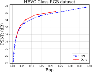
(a) Intra Period 32

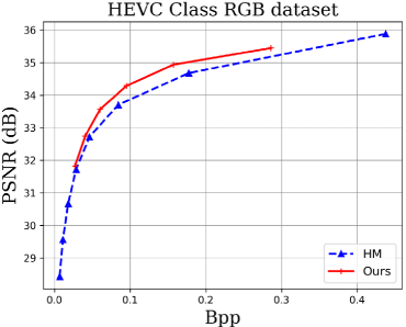
(b) Intra Period 12

Figure 12: Rate-distortion performance of our proposed scheme on the HEVC Class RGB dataset when the bit rate is extended to lower and higher.

IV-C5 Wider Bit Rate Range

It is a common practice to train four models with different bit rate in previous learned video codecs. To make it easier to compare with the previous learned video codecs, our proposed scheme follows the same setting. However, it is still necessary to explore whether the learned video codecs are well-performed in band-limited (lower bit rate) and broadband (higher bit rate) environments. Therefore, when oriented to PSNR, we set $\lambda$ to 128 and 4096 to train additional two models. When oriented to MS-SSIM, we set $\lambda$ to 4 and 128. For other learned video codecs (DVC_Pro [4], MLVC [9], RLVC [16], DCVC [27]), since their officially released models only support four bit rate points, we can not extend their bit rate ranges. Fig. 12 illustrates the rate-distortion performance of our proposed scheme on the HEVC Class RGB when the bit rate is extended to lower and higher. The results show that our scheme can still work well over a wider range of bit rates.

V Conclusion and Discussion

In this paper, we propose a temporal context mining module and a temporal context re-filling procedure to better learn and utilize temporal contexts for learned video compression. Without the auto-regressive entropy model, our proposed scheme achieves higher compression ratio than the existing learned video codecs. Our scheme also outperforms the reference software of H.265/HEVC—HM in terms of PSNR by 14.4% and outperforms the reference software of H.266/VVC—VTM in terms of MS-SSIM by 21.1%. Even the proposed scheme outperforms VTM with the highest-compression-ratio settings for low-delay coding in terms of MS-SSIM, it is far behind than VTM in terms of PSNR. In addition, the complexity, especially the decoding complexity still needs to be significantly reduced before it can be used in practice. We will further investigate it in our future work.

Xihua Sheng received the B.S. degree in automation from Northeastern University, Shenyang, China, in 2019. He is currently pursuing the Ph.D. degree in the Department of Electronic Engineering and Information Science at the University of Science and Technology of China, Hefei, China. His research interests include image/video/point cloud coding, signal processing, and machine learning.

Jiahao Li received the B.S. degree in computer science and technology from the Harbin Institute of Technology in 2014, and the Ph.D. degree from Peking University in 2019. He is currently a Senior Researcher with the Media Computing Group, Microsoft Research Asia. Previously, he worked on video coding and has more than ten published papers, standard proposals, and patents in this area. His current research interests mainly focus on neural video compression and real-time communication.

Bin Li received the B.S. and Ph.D. degrees in electronic engineering from the University of Science and Technology of China (USTC), Hefei, Anhui, China, in 2008 and 2013, respectively. He joined Microsoft Research Asia (MSRA), Beijing, China, in 2013 and now he is a Principal Researcher. He has authored or co-authored over 50 papers. He holds over 30 granted or pending U.S. patents in the area of image and video coding. He has more than 40 technical proposals that have been adopted by Joint Collaborative Team on Video Coding. His current research interests include video coding, processing, transmission, and communication. Dr. Li received the best paper award for the International Conference on Mobile and Ubiquitous Multimedia from Association for Computing Machinery in 2011. He received the Top 10% Paper Award of 2014 IEEE International Conference on Image Processing. He received the best paper award of IEEE Visual Communications and Image Processing 2017.

Li Li (M’17) received the B.S. and Ph.D. degrees in electronic engineering from University of Science and Technology of China (USTC), Hefei, Anhui, China, in 2011 and 2016, respectively. He was a visiting assistant professor in University of Missouri-Kansas City from 2016 to 2020. He joined the department of electronic engineering and information science of USTC as a research fellow in 2020 and became a professor in 2022. His research interests include image/video/point cloud coding and processing. He received the Best 10% Paper Award at the 2016 IEEE Visual Communications and Image Processing (VCIP) and the 2019 IEEE International Conference on Image Processing (ICIP).

Dong Liu (M’13–SM’19) received the B.S. and Ph.D. degrees in electrical engineering from the University of Science and Technology of China (USTC), Hefei, China, in 2004 and 2009, respectively. He was a Member of Research Staff with Nokia Research Center, Beijing, China, from 2009 to 2012. He joined USTC as a faculty member in 2012 and became a Professor in 2020. His research interests include image and video processing, coding, analysis, and data mining. He has authored or co-authored more than 200 papers in international journals and conferences. He has more than 20 granted patents. He has several technical proposals adopted by international or domestic standardization groups. He received the 2009 IEEE Transactions on Circuits and Systems for Video Technology Best Paper Award and the VCIP 2016 Best 10% Paper Award. He and his students were winners of several technical challenges held in ISCAS 2022, ICCV 2019, ACM MM 2019, ACM MM 2018, ECCV 2018, CVPR 2018, and ICME 2016. He is a Senior Member of CCF and CSIG, an elected member of MSA-TC of IEEE CAS Society. He serves or had served as the Chair of IEEE 1857.11 Standard Working Subgroup, a Guest Editor for IEEE Transactions on Circuits and Systems for Video Technology, an Associate Editor for Frontiers in Signal Processing, an Organizing Committee member for VCIP 2022, ICME 2021, ICME 2019, etc.

Yan Lu received his Ph.D. degree in computer science from Harbin Institute of Technology, China. He joined Microsoft Research Asia in 2004, where he is now a Partner Research Manager and manages research on media computing and communication. He and his team have transferred many key technologies and research prototypes to Microsoft products. From 2001 to 2004, he was a team lead of video coding group in the JDL Lab, Institute of Computing Technology, China. From 1999 to 2000, he was with the City University of Hong Kong as a research assistant. Yan Lu has broad research interests in the fields of real-time communication, computer vision, video analytics, audio enhancement, virtualization, and mobile-cloud computing. He holds 30+ granted US patents and has published 100+ papers in refereed journals and conference proceedings.

References

- [1] T. Wiegand, G. J. Sullivan, G. Bjontegaard, and A. Luthra, “Overview of the H.264/AVC video coding standard,” IEEE Transactions on Circuits and Systems for Video Technology, vol. 13, no. 7, pp. 560–576, 2003.
- [2] G. J. Sullivan, J.-R. Ohm, W.-J. Han, and T. Wiegand, “Overview of the high efficiency video coding (HEVC) standard,” IEEE Transactions on Circuits and Systems for Video Technology, vol. 22, no. 12, pp. 1649–1668, 2012.
- [3] B. Bross, Y.-K. Wang, Y. Ye, S. Liu, J. Chen, G. J. Sullivan, and J.-R. Ohm, “Overview of the versatile video coding (VVC) standard and its applications,” IEEE Transactions on Circuits and Systems for Video Technology, 2021.
- [4] G. Lu, X. Zhang, W. Ouyang, L. Chen, Z. Gao, and D. Xu, “An end-to-end learning framework for video compression,” IEEE Transactions on Pattern Analysis and Machine Intelligence, 2020.
- [5] O. Rippel, A. G. Anderson, K. Tatwawadi, S. Nair, C. Lytle, and L. Bourdev, “ELF-VC: Efficient learned flexible-rate video coding,” in Proceedings of the IEEE/CVF International Conference on Computer Vision (ICCV), pp. 14479–14488, October 2021.
- [6] H. Liu, H. Shen, L. Huang, M. Lu, T. Chen, and Z. Ma, “Learned video compression via joint spatial-temporal correlation exploration,” in Proceedings of the AAAI Conference on Artificial Intelligence, vol. 34, pp. 11580–11587, 2020.
- [7] Z. Hu, Z. Chen, D. Xu, G. Lu, W. Ouyang, and S. Gu, “Improving deep video compression by resolution-adaptive flow coding,” in European Conference on Computer Vision (ECCV), pp. 193–209, Springer, 2020.
- [8] G. Lu, C. Cai, X. Zhang, L. Chen, W. Ouyang, D. Xu, and Z. Gao, “Content adaptive and error propagation aware deep video compression,” in European Conference on Computer Vision (ECCV), pp. 456–472, Springer, 2020.
- [9] J. Lin, D. Liu, H. Li, and F. Wu, “M-LVC: multiple frames prediction for learned video compression,” in Proceedings of the IEEE/CVF Conference on Computer Vision and Pattern Recognition (CVPR), pp. 3546–3554, 2020.
- [10] Z. Hu, G. Lu, and D. Xu, “FVC: A new framework towards deep video compression in feature space,” in Proceedings of the IEEE/CVF Conference on Computer Vision and Pattern Recognition (CVPR), pp. 1502–1511, 2021.
- [11] R. Yang, F. Mentzer, L. V. Gool, and R. Timofte, “Learning for video compression with hierarchical quality and recurrent enhancement,” in Proceedings of the IEEE/CVF Conference on Computer Vision and Pattern Recognition (CVPR), pp. 6628–6637, 2020.
- [12] E. Agustsson, D. Minnen, N. Johnston, J. Balle, S. J. Hwang, and G. Toderici, “Scale-space flow for end-to-end optimized video compression,” in Proceedings of the IEEE/CVF Conference on Computer Vision and Pattern Recognition (CVPR), pp. 8503–8512, 2020.
- [13] Z. Cheng, H. Sun, M. Takeuchi, and J. Katto, “Learning image and video compression through spatial-temporal energy compaction,” in Proceedings of the IEEE/CVF Conference on Computer Vision and Pattern Recognition (CVPR), pp. 10071–10080, 2019.
- [14] O. Rippel, S. Nair, C. Lew, S. Branson, A. G. Anderson, and L. Bourdev, “Learned video compression,” in Proceedings of the IEEE/CVF International Conference on Computer Vision (ICCV), pp. 3454–3463, 2019.
- [15] A. Djelouah, J. Campos, S. Schaub-Meyer, and C. Schroers, “Neural inter-frame compression for video coding,” in Proceedings of the IEEE/CVF International Conference on Computer Vision (ICCV), pp. 6421–6429, 2019.
- [16] R. Yang, F. Mentzer, L. Van Gool, and R. Timofte, “Learning for video compression with recurrent auto-encoder and recurrent probability model,” IEEE Journal of Selected Topics in Signal Processing, vol. 15, no. 2, pp. 388–401, 2021.
- [17] C.-Y. Wu, N. Singhal, and P. Krahenbuhl, “Video compression through image interpolation,” in Proceedings of the European Conference on Computer Vision (ECCV), pp. 416–431, 2018.
- [18] B. Liu, Y. Chen, S. Liu, and H.-S. Kim, “Deep learning in latent space for video prediction and compression,” in Proceedings of the IEEE/CVF Conference on Computer Vision and Pattern Recognition (CVPR), pp. 701–710, 2021.
- [19] H. Liu, M. Lu, Z. Ma, F. Wang, Z. Xie, X. Cao, and Y. Wang, “Neural video coding using multiscale motion compensation and spatiotemporal context model,” IEEE Transactions on Circuits and Systems for Video Technology, 2020.
- [20] M. A. Yılmaz and A. M. Tekalp, “End-to-end rate-distortion optimized learned hierarchical bi-directional video compression,” IEEE Transactions on Image Processing, vol. 31, pp. 974–983, 2021.
- [21] Z. Chen, T. He, X. Jin, and F. Wu, “Learning for video compression,” IEEE Transactions on Circuits and Systems for Video Technology, vol. 30, no. 2, pp. 566–576, 2019.
- [22] S. Ma, X. Zhang, C. Jia, Z. Zhao, S. Wang, and S. Wang, “Image and video compression with neural networks: A review,” IEEE Transactions on Circuits and Systems for Video Technology, vol. 30, no. 6, pp. 1683–1698, 2019.
- [23] A. Habibian, T. v. Rozendaal, J. M. Tomczak, and T. S. Cohen, “Video compression with rate-distortion autoencoders,” in Proceedings of the IEEE/CVF International Conference on Computer Vision (ICCV), October 2019.
- [24] W. Sun, C. Tang, W. Li, Z. Yuan, H. Yang, and Y. Liu, “High-quality single-model deep video compression with frame-conv3d and multi-frame differential modulation,” in European Conference on Computer Vision (ECCV), pp. 239–254, Springer, 2020.
- [25] J. Pessoa, H. Aidos, P. Tomás, and M. A. Figueiredo, “End-to-end learning of video compression using spatio-temporal autoencoders,” in 2020 IEEE Workshop on Signal Processing Systems (SiPS), pp. 1–6, IEEE, 2020.
- [26] J. Liu, S. Wang, W.-C. Ma, M. Shah, R. Hu, P. Dhawan, and R. Urtasun, “Conditional entropy coding for efficient video compression,” in European Conference on Computer Vision (ECCV), pp. 453–468, Springer, 2020.
- [27] J. Li, B. Li, and Y. Lu, “Deep contextual video compression,” Advances in Neural Information Processing Systems, vol. 34, pp. 18114–18125, 2021.
- [28] J. Wang, X. Deng, M. Xu, C. Chen, and Y. Song, “Multi-level wavelet-based generative adversarial network for perceptual quality enhancement of compressed video,” in European Conference on Computer Vision (ECCV), pp. 405–421, Springer, 2020.
- [29] R. Yang, R. Timofte, and L. Van Gool, “Perceptual learned video compression with recurrent conditional gan,” in Proceedings of the Thirty-First International Joint Conference on Artificial Intelligence, IJCAI-22, pp. 1537–1544, International Joint Conferences on Artificial Intelligence Organization, 7 2022.
- [30] W. Ding, F. Wu, X. Wu, S. Li, and H. Li, “Adaptive directional lifting-based wavelet transform for image coding,” IEEE Transactions on Image Processing, vol. 16, no. 2, pp. 416–427, 2007.
- [31] F. Wu, S. Li, and Y.-Q. Zhang, “A framework for efficient progressive fine granularity scalable video coding,” IEEE Transactions on Circuits and Systems for Video Technology., vol. 11, pp. 332–344, 2001.
- [32] H. Ma, D. Liu, N. Yan, H. Li, and F. Wu, “End-to-end optimized versatile image compression with wavelet-like transform,” IEEE Transactions on Pattern Analysis and Machine Intelligence, 2020.
- [33] “x265.” https://www.videolan.org/developers/x265.html. Accessed: 2022-07-05.
- [34] “JM-19.0.” http://iphome.hhi.de/suehring/. Accessed: 2022-07-05.
- [35] “HM-16.20.” https://vcgit.hhi.fraunhofer.de/jvet/HM/. Accessed: 2022-07-05.
- [36] “VTM-13.2.” https://vcgit.hhi.fraunhofer.de/jvet/VVCSoftware_VTM/. Accessed: 2022-03-02.
- [37] R. Yang, Y. Yang, J. Marino, and S. Mandt, “Hierarchical autoregressive modeling for neural video compression,” in 9th International Conference on Learning Representations, ICLR 2021, Virtual Event, Austria, May 3-7, 2021, OpenReview.net, 2021.
- [38] D. Minnen, J. Ballé, and G. Toderici, “Joint autoregressive and hierarchical priors for learned image compression,” in Advances in Neural Information Processing Systems 31: Annual Conference on Neural Information Processing Systems 2018, NeurIPS 2018, December 3-8, 2018, Montréal, Canada, pp. 10794–10803, 2018.
- [39] Z. Wang, E. P. Simoncelli, and A. C. Bovik, “Multiscale structural similarity for image quality assessment,” in The Thrity-Seventh Asilomar Conference on Signals, Systems & Computers, 2003, vol. 2, pp. 1398–1402, Ieee, 2003.
- [40] Z. Guo, Z. Zhang, R. Feng, and Z. Chen, “Causal contextual prediction for learned image compression,” IEEE Transactions on Circuits and Systems for Video Technology, 2021.
- [41] Z. Cheng, H. Sun, M. Takeuchi, and J. Katto, “Learned image compression with discretized gaussian mixture likelihoods and attention modules,” in Proceedings of the IEEE Conference on Computer Vision and Pattern Recognition (CVPR), 2020.
- [42] “x264.” https://www.videolan.org/developers/x264.html. Accessed: 2022-07-05.
- [43] F. Mentzer, E. Agustsson, J. Ballé, D. Minnen, N. Johnston, and G. Toderici, “Neural video compression using gans for detail synthesis and propagation,” in European Conference on Computer Vision, pp. 562–578, Springer, 2022.
- [44] A. Ranjan and M. J. Black, “Optical flow estimation using a spatial pyramid network,” in Proceedings of the IEEE/CVF Conference on Computer Vision and Pattern Recognition (CVPR), pp. 4161–4170, 2017.
- [45] J. Ballé, D. Minnen, S. Singh, S. J. Hwang, and N. Johnston, “Variational image compression with a scale hyperprior,” in 6th International Conference on Learning Representations, ICLR 2018, Vancouver, BC, Canada, April 30 - May 3, 2018, Conference Track Proceedings, OpenReview.net, 2018.
- [46] J. Bégaint, F. Racapé, S. Feltman, and A. Pushparaja, “Compressai: a pytorch library and evaluation platform for end-to-end compression research,” arXiv preprint arXiv:2011.03029, 2020.
- [47] R. Feng, Y. Wu, Z. Guo, Z. Zhang, and Z. Chen, “Learned video compression with feature-level residuals,” in Proceedings of the IEEE/CVF Conference on Computer Vision and Pattern Recognition Workshops, pp. 120–121, 2020.
- [48] K. He, X. Zhang, S. Ren, and J. Sun, “Deep residual learning for image recognition,” in Proceedings of the IEEE Conference on Computer Vision and Pattern recognition (CVPR), pp. 770–778, 2016.
- [49] W. Shi, J. Caballero, F. Huszár, J. Totz, A. P. Aitken, R. Bishop, D. Rueckert, and Z. Wang, “Real-time single image and video super-resolution using an efficient sub-pixel convolutional neural network,” in Proceedings of the IEEE/CVF Conference on Computer Vision and Pattern Recognition (CVPR), pp. 1874–1883, 2016.
- [50] K. Zhang, W. Zuo, Y. Chen, D. Meng, and L. Zhang, “Beyond a gaussian denoiser: Residual learning of deep cnn for image denoising,” IEEE Transactions on Image Processing, vol. 26, no. 7, pp. 3142–3155, 2017.
- [51] Z. Guo, R. Feng, Z. Zhang, X. Jin, and Z. Chen, “Learning cross-scale prediction for efficient neural video compression,” arXiv preprint arXiv:2112.13309, 2021.
- [52] D. Flynn, D. Marpe, M. Naccari, T. Nguyen, C. Rosewarne, K. Sharman, J. Sole, and J. Xu, “Overview of the range extensions for the hevc standard: Tools, profiles, and performance,” IEEE Transactions on Circuits and Systems for Video Technology, vol. 26, no. 1, pp. 4–19, 2015.
- [53] D. Ma, F. Zhang, and D. Bull, “BVI-DVC: A training database for deep video compression,” IEEE Transactions on Multimedia, 2021.
- [54] A. V. Katsenou, G. Dimitrov, D. Ma, and D. R. Bull, “Bvi-syntex: A synthetic video texture dataset for video compression and quality assessment,” IEEE Transactions on Multimedia, vol. 23, pp. 26–38, 2020.
- [55] T. Xue, B. Chen, J. Wu, D. Wei, and W. T. Freeman, “Video enhancement with task-oriented flow,” International Journal of Computer Vision, vol. 127, no. 8, pp. 1106–1125, 2019.
- [56] A. Mercat, M. Viitanen, and J. Vanne, “UVG dataset: 50/120fps 4k sequences for video codec analysis and development,” in Proceedings of the 11th ACM Multimedia Systems Conference, pp. 297–302, 2020.
- [57] H. Wang, W. Gan, S. Hu, J. Y. Lin, L. Jin, L. Song, P. Wang, I. Katsavounidis, A. Aaron, and C.-C. J. Kuo, “MCL-JCV: a JND-based H.264/AVC video quality assessment dataset,” in 2016 IEEE International Conference on Image Processing (ICIP), pp. 1509–1513, IEEE, 2016.
- [58] I. Loshchilov and F. Hutter, “Decoupled weight decay regularization,” in 7th International Conference on Learning Representations, ICLR 2019, New Orleans, LA, USA, May 6-9, 2019, OpenReview.net, 2019.
- [59] G. Bjontegaard, “Calculation of average psnr differences between rd-curves,” VCEG-M33, 2001.