Adaptive Perturbation for Adversarial Attack

Abstract

In recent years, the security of deep learning models achieves more and more attentions with the rapid development of neural networks, which are vulnerable to adversarial examples. Almost all existing gradient-based attack methods use the sign function in the generation to meet the requirement of perturbation budget on $L_{\infty}$ norm. However, we find that the sign function may be improper for generating adversarial examples since it modifies the exact gradient direction. Instead of using the sign function, we propose to directly utilize the exact gradient direction with a scaling factor for generating adversarial perturbations, which improves the attack success rates of adversarial examples even with fewer perturbations. At the same time, we also theoretically prove that this method can achieve better black-box transferability. Moreover, considering that the best scaling factor varies across different images, we propose an adaptive scaling factor generator to seek an appropriate scaling factor for each image, which avoids the computational cost for manually searching the scaling factor. Our method can be integrated with almost all existing gradient-based attack methods to further improve their attack success rates. Extensive experiments on the CIFAR10 and ImageNet datasets show that our method exhibits higher transferability and outperforms the state-of-the-art methods.

1 Introduction

With the rapid progress and significant success in the deep learning in recent years, its security issue has attracted more and more attention. One of the most concerned security problems is its vulnerability to small, human-imperceptible adversarial noise [1], which implies severe risk of being attacked intentionally especially for technologies like face recognition and automatic driving. While it is important to study how to strengthen deep learning models to defend adversarial attack, it is equally important to explore how to attack these models.

Existing attack methods generate an adversarial example by adding to input some elaborately designed adversarial perturbations, which are usually generated either by a generative network [2, 3, 4, 5, 6, 7] or by the gradient-based optimization [8, 9, 10, 11, 12, 13, 14]. The latter, i.e., gradient-based methods, are the mainstream. Their key idea is generating the perturbation by exploiting the gradient computed via maximizing the loss function of the target task.

In these methods, since the gradient varies in different pixels, the sign function is usually used to normalize the gradient, which is convenient to set the step size of each step during the attack. Under the most commonly used $L_{\infty}$ norm setting in the adversarial attack, i.e., constraining the maximal $L_{\infty}$ norm of the generated adversarial perturbations, the use of the sign function can also leverage the largest perturbation budget to enhance the aggressiveness of adversarial examples. Due to the influence of the sign function, all values of the gradient are normalized into $\{0,+1,-1\}$. Although this approach can scale the gradient value, so as to make full use of the perturbation budget in the $L_{\infty}$ attack, the resultant update directions in adversarial attack are limited, there are only eight possible update directions in the case of a two-dimensional space. The inaccurate update direction may cause the generated adversarial examples to be sub-optimal (as shown in Fig. 1).

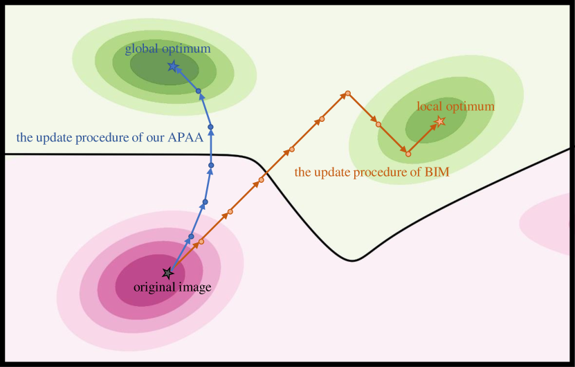
Figure 1: A two-dimensional toy example to illustrate the difference between our proposed APAA and existing sign-based methods, e.g., BIM [9]. The orange path and blue path represent the update procudure of BIM and our APAA when generating adversarial examples, respectively. The background color represents the contour of the classification loss function. During the adversarial attack, we aim to achieve an adversarial example with a larger loss function. Due to the limitation of the sign function, there are only eight possible update directions in the case of a two-dimensional space ((0, 1), (0, -1), (1, 1), (1, -1), (1, 0), (-1, -1), (-1, 0), (-1, 1)). The update direction of BIM is limited and not accurate enough, resulting in only reaching the sub-optimal end-point. Our method can not only obtain a more accurate update direction, but also adjust the step size adaptively. As a result, our APAA may reach the global optimum with a larger probability in fewer steps.

To solve the above problem of existing methods, we propose a method called Adaptive Perturbation for Adversarial Attack (APAA), which directly multiplies a scaling factor to the gradient of loss function instead of using the sign function to normalize. The scaling factor can either be elaborately selected manually, or adaptively generated according to different image characteristics. Specifically, to further take the characteristics of different images into consideration, we propose an adaptive scaling factor generator to automatically generate the suitable scaling factor in each attack step during the generation of adversarial examples. From Fig. 1, we can clearly see that, since our method can adaptively adjust the step size in each attack step, a large step size can be used in the first few steps of iterative attacks to make full use of the perturbation budget, and when close to the global optimal point, the step size can be adaptively reduced. With more accurate update direction, our APAA may reach the global optimum with fewer update steps and perturbations, which means the generated adversarial examples are more aggressive and thus can improve the corresponding attack success rate.

Adversarial examples have an intriguing property of transferability, where adversarial examples generated by one model can also fool other unknown models. Wang et al. [15] discover the negative correlation between the adversarial transferability and the interaction inside adversarial perturbations. Based on their findings, we theoretically demonstrate that the adversarial examples generated by our APAA method have better black-box transferability.

The main contributions of our work are as follows:

1. We propose an effective attack method by directly multiplying the gradient of loss function by a scaling factor instead of employing the sign function, which is nearly used in all existing gradient-based methods to normalize the gradient.

2. We propose an adaptive scaling factor generator to generate the suitable scaling factor in each attack step according to the characteristics of different images, which gets rid of manually hyperparameter searching.

3. We theoretically demonstrate that the adversarial examples generated by our method achieve better black-box transferability.

4. Extensive experiments on the datasets of CIFAR10 and ImageNet show the superiority of our proposed method. Our method significantly improves the transferability of generated adversarial examples and achieves higher attack success rates on both white-box and black-box settings than the state-of-the-art methods with fewer update steps and perturbations budgets.

2 Related Work

The phenomenon of adversarial examples is proposed by Szegedy et al. [1]. The attack and defense methods promote the development of each other in recent years, which are briefly reviewed in this section, respectively.

2.1 Attack Methods

The attack methods mainly consist of the generative-based [2, 3, 4, 5, 6, 7] and gradient-based methods [8, 9, 10, 11, 12, 13, 14], and the latter ones are the mainstream. Our work mainly focuses on the gradient-based attack methods under the setting of $L_{\infty}$ norm. Before introducing the methods in detail, we first introduce some notations that will be used later. Let $x$ and $y$ be the original image and its corresponding class label, respectively. Let $J(x,y)$ be the loss function of cross-entropy. Let $x_{adv}$ be the generated adversarial example. Let $\epsilon$ and $\alpha$ be the total perturbation budget and the budget in each step of the iterative methods. $\Pi_{x,\epsilon}$ means to clip the generated adversarial examples within the $\epsilon$-neighborhood of the original image on $L_{\infty}$ norm.

Fast Gradient Sign Method. FGSM [8] is a one-step method for white-box attack, which directly utilizes the gradient of loss function to generate the adversarial example:

$$x^{adv}=x+\epsilon\cdot\mathrm{sign}(\nabla_{x}J(f(x),y)).$$ (1)

Basic Iterative Method. BIM [9] is an extension of FGSM, which uses the iterative method to improve the attack success rate of adversarial examples:

$$x^{adv}_{t+1}=\Pi_{x,\epsilon}(x^{adv}_{t}+\alpha\cdot\mathrm{sign}(\nabla_{x}J(f(x^{adv}_{t}),y))),$$ (2)

where $x^{adv}_{0}=x$ and the subscript $t$ is the index of iteration.

Momentum Iterative Fast Gradient Sign Method. MIFGSM [11] proposes a momentum term to accumulate the gradient in previous steps to achieve more stable update directions, which greatly improves the transferability of generated adversarial examples:

$$g_{t+1}=\mu\cdot g_{t}+\frac{\nabla_{x}J(f(x^{adv}_{t}),y)}{\|\nabla_{x}J(f(x^{adv}_{t}),y)\|_{1}},$$ (3)

$$x^{adv}_{t+1}=\Pi_{x,\epsilon}(x^{adv}_{t}+\alpha\cdot\mathrm{sign}(g_{t+1})),$$ (4)

where $g_{t}$ denotes the momentum item of gradient in the $t$-th iteration and $\mu$ is a decay factor.

Since then, various methods have been further proposed to improve the transferability of adversarial examples. A randomization operation of random resizing and zero-padding to the original image is proposed in DIM [12]. TIM [13] proposes a translation-invariant attack method by convolving the gradient with a Gaussian kernel to further improve the transferability of adversarial examples. Inspired by Nesterov accelerated gradient [16], SIM [14] amends the accumulation of the gradients to effectively look ahead and improve the transferability of adversarial examples. In addition, SIM also proposes to use several copies of the original image with different scales to generate the adversarial example. SGM [17] finds that using more gradients from the skip connections rather than the residual modules can craft adversarial examples with higher transferability. VT [18] considers the gradient variance of the previous iteration to tune the current gradient so as to stabilize the update direction and escape from poor local optima. EMI [19] accumulates the gradients of data points sampled in the gradient direction of previous iteration to find more stable direction of the gradient. IR [15] discovers the negative correlation between the adversarial transferability and the interaction inside adversarial perturbations and proposes to directly penalize interactions during the attacking process, which significantly improves the adversarial transferability. AIFGTM [20] also considers the limitations of the basic sign structure and proposes an ADAM iterative fast gradient tanh method to generate indistinguishable adversarial examples with high transferability.

2.2 Defense Methods

Adversarial defense aims to improve the robustness of the target model in the case of adversarial examples being the inputs. The defense methods can mainly be categorized into adversarial training, input transformation, model ensemble, and certified defenses. The adversarial training methods [10, 21, 22, 23, 24] use the adversarial examples as the extra training datas to improve the robustness of the model. The input transformation methods [25, 26, 27, 28, 29] tend to denoise the adversarial examples before feeding them into the classifier. The model ensemble methods [30, 31, 32] use multiple models simultaneously to reduce the influence of adversarial examples on the single model and achieve more robust results. Certified defense methods [33, 34, 35, 36] guarantee that the target model can correctly classify the adversarial examples within the given distance from the original images.

3 Method

In this section, we first analyze the defect of the sign function used in existing gradient-based attack methods in Sec. 3.1. Then we propose our method of Adaptive Perturbation for Adversarial Attack (APAA) in Sec. 3.2, i.e., utilizing a scaling factor to multiply the gradient instead of the sign function normalization. The scaling factor can either be elaborately selected manually (in Sec. 3.2.1), or adaptively generated according to different image characteristics by a generator (in Sec. 3.2.2). Finally, we theoretically demonstrate that our proposed method can improve the black-box transferability of adversarial examples in Sec. 3.3.

3.1 Rethinking the Sign Function

The task of adversarial attack is to do a minor modification on the original images with human-imperceptible noises to fool the target model, i.e., misclassifying the adversarial examples. The gradient-based methods generate the adversarial examples by maximizing the cross-entropy loss function, which can be formulated as follows:

$$\mathop{\arg\max}_{x^{adv}}J(f(x^{adv}),y),\quad\mathrm{s.t.}\|x^{adv}-x\|_{p}\leq\epsilon,$$ (5)

where $p$ could be $0,1,2$ and $\infty$.

Since the gradient varies in different pixels, the sign function is usually used to normalize the gradient, which is convenient to set the step size of each step during the attack (e.g., Eq. 1). Under the most commonly used $L_{\infty}$ norm setting in the adversarial attack, i.e., constraining the maximal $L_{\infty}$ norm of the generated adversarial perturbations, the use of the sign function can also leverage the largest perturbation budget to enhance the aggressiveness of adversarial examples.

The sign function normalizes all values of the gradient into $\{0,+1,-1\}$. Although this method can scale the gradient value to make full use of the perturbation budget in the $L_{\infty}$ attack, the resultant update directions in adversarial attack are limited, e.g., there are only eight possible update directions in the case of a two-dimensional space ((0, 1), (0, -1), (1, 1), (1, -1), (1, 0), (-1, -1), (-1, 0), (-1, 1)). From Fig. 1, we can clearly see that the attack directions in sign-based methods (e.g., BIM [9]) are distracted and not accurate anymore, which conversely needs more update steps and perturbations budgets to implement a successful attack. The inaccurate update direction may cause the generated adversarial examples to be sub-optimal.

3.2 Adaptive Perturbation for Adversarial Attack

To solve the problem mentioned above, we propose a method of Adaptive Perturbation for Adversarial Attack (APAA). Specifically, we propose to directly multiply the gradient by a scaling factor instead of normalizing it with the sign function. The scaling factor can be determined either elaborately selected manually, or adaptively achieved from a generator according to different image characteristics. We will introduce each of them in the following, respectively.

3.2.1 Fixed Scaling Factor

First, we propose to directly multiply the gradient by a fixed scaling factor, which not only maintains the accurate gradient directions but also can flexibly utilize the perturbation budget through the adjustment of the scaling factor:

$$x^{adv}_{t+1}=\Pi_{x,\epsilon}(x^{adv}_{t}+\gamma\cdot\nabla_{x}J(f(x^{adv}_{t}),y)),$$ (6)

where $\gamma$ is the scaling factor, $\Pi_{x,\epsilon}$ means to clip the generated adversarial examples within the $\epsilon$-neighborhood of the original image on $L_{\infty}$ norm.

Our method is easy to implement and can be combined with all existing gradient-based attack methods (e.g., MIFGSM [11], DIM [12], TIM [13], SIM [14]). We take the MIFGSM method as an example. When integrating with MIFGSM, the full update formulation is as follows:

$$x_{0}^{adv}=x,$$ (7)

$$g_{t+1}=\mu\cdot g_{t}+\frac{\nabla_{x}J(f(x^{adv}_{t}),y)}{\|\nabla_{x}J(f(x^{adv}_{t}),y)\|_{1}},$$ (8)

$$x^{adv}_{t+1}=\Pi_{x,\epsilon}(x_{t}^{adv}+\gamma\cdot g_{t+1}),$$ (9)

where $\mu$ is the decay factor in MIFGSM, $\gamma$ is the scaling factor.

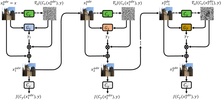
Figure 2: The overview of the scaling factor generator. In each step $t$, the gradient of one randomly selected model $C_{x}$ is first calculated. Simultaneously, the adversarial example from the previous step together with the gradient information are fed into the generator $G_{t}$ to generate the scaling factor $\gamma_{t}$. Then the scaling factor and the gradient information are used to generate the adversarial perturbation. The adversarial examples generated in all steps are all fed into another classifier $C_{y}$ to optimize the parameters of generator $G_{t}$ through maximizing the cross-entropy loss between the output classification probability and the ground truth label.

3.2.2 Adaptive Scaling Factor

Considering that suitable scaling factors vary across different images, we further propose a generator to directly generate the adaptive scaling factor in each step of adversarial examples generation, which also gets rid of manually hyperparameter searching.

The overview of our proposed adaptive scaling factor generator is shown in Fig. 2. We employ an iterative method to generate the adversarial example with $T$ steps. In each step $t$, the gradient of the adversarial examples generated in the previous step is calculated through a randomly selected white-box model $C_{x}$. The corresponding scaling factor is also generated through the generator $G_{t}$ by feeding the adversarial example together with the gradient information as the input. Then the gradient information and scaling factor are used to generate the new adversarial perturbation. We used the BIM-style update method ($x_{t}^{adv}=x_{t-1}^{adv}+\gamma_{t}\cdot\nabla_{x}J(C_{x}(x_{t-1}^{adv}),y)$) as an example in the figure for convenience, but in fact any existing gradient-based attack method can be utilized. The generated adversarial examples in all steps are used to calculate the cross-entropy loss by another classifier $C_{y}$. Then the parameters in the generator $G_{t}$ are updated by maximizing the cross-entropy loss through backpropagation, aiming to generate the adversarial examples, which can mislead the classifier. The generators used in each step share the same architecture but do not share the parameters. The procedure of training the generator is summarized in Algorithm 1.

Algorithm 1 The training of adaptive scaling factor generator

1:the total training step $N$

2:the number of attack iteration $T$

3:the learning rate $\beta$

4:the dataset $(\mathcal{X,Y})$

5:the white-box models $C_{1},\cdots,C_{n}$

6:the scaling factor generators $G_{1},G_{2},\cdots,G_{T}$ with the parameters of $\theta$

7:for i $\in\{1,\cdots N\}$  do

8:     Sample the image and label pair $(x,y)$ from $(\mathcal{X,Y})$

9:     Randomly choose two classifiers $C_{x}$ and $C_{y}$ from $C_{1},\cdots,C_{n}$

10:     $x_{0}^{adv}=x$

11:     for t $\in\{1,\cdots T\}$  do

12:         $grad_{t}=\nabla_{x}J(C_{x}(x_{t-1}^{adv}),y)$

13:         $\gamma_{t}=G_{t}(x_{t-1}^{adv},grad_{t})$

14:         $x_{t}^{adv}=\Pi_{x,\epsilon}(\gamma_{t}\cdot grad_{t}+x_{t-1}^{adv})$ $\triangleright$ using the update in BIM as an example

15:         $loss_{t}=J(C_{y}(x_{t}^{adv}),y)$

16:         $G_{t}(\theta)=G_{t}(\theta)+\beta\cdot\nabla_{\theta}(loss_{t})$

17:     end for

18:end for

As shown in Fig. 1, compared to the sign-based methods, our proposed APAA can adaptively adjust the step size in each attack step. A large step size can be used in the first few steps of iterative attacks to make full use of the perturbation budget, and when close to the global optimal point, the step size can be adaptively reduced. With more accurate update direction, our APAA may reach the global optimum with fewer update steps and perturbations, which means the generated adversarial examples are more aggressive and thus can improve the corresponding attack success rate.

3.3 Theoretical Analysis

Adversarial examples have an intriguing property of transferability, where adversarial examples generated by one model can also fool other unknown models. In addition to the intuitive idea to illustrate that our method can provide more accurate attack directions, we also provide a theoretical proof to show that our proposed method can meanwhile improve the black-box transferability of adversarial examples. Wang et al. [15] utilizes the Shapley interaction index proposed in game theory [37, 38] to analyze the interactions inside adversarial perturbations. Through extensive experiments, they discover the negative correlation between the adversarial transferability and the interaction inside adversarial perturbations. Based on their findings, we theoretically demonstrate that the adversarial examples generated by our APAA method have better black-box transferability.

Shapley value [38] was first proposed in game theory in 1953. In a multiplayer game, players work together to obtain a high reward. Shapley Value is used to distribute the rewards shared by everyone according to each player’s contribution fairly. $\Omega=\{1,2,\cdots,n\}$ represents the set of all players, $v(\cdot)$ represents the reward function, $\phi(i|\Omega)$ represents an unbiased estimate of the contribution of the i-th player to all players $\Omega$, which can be calculated as follows:

$$\phi(i|\Omega)=\sum_{S\subseteq\Omega\backslash\{i\}}\frac{|S|!(n-|S|-1)!}{n!}(v(S\cup\{i\})-v(S)).$$ (10)

When applying the Shapley value into the adversarial examples, $\phi(i|\Omega)$ is used to measure the contribution of each perturbed pixel $i\in\Omega$ to the attack. During the adversarial examples, the reward function can be definded as:

$$v(S)=\max_{y^{\prime}\neq y}h_{y^{\prime}}(x+\delta^{(S)})-h_{y}(x+\delta^{(S)}),$$ (11)

where $h_{y}(\cdot)$ represents the y-th element in the logits layer of DNN model, $y$ is the gound truth label of input image $x$, $\delta^{(S)}$ is the perturbation which only contains perturbation units in $S$, i.e., $\forall i\in S,\delta_{i}^{(S)}=\delta_{i};\forall i\notin S,\delta_{i}^{(S)}=0$. According to [37] the Shapley interaction index between units $i$ and $j$ is defined as follows:

$$I_{ij}(\delta)=\phi(S_{ij}|\Omega^{\prime})-[\phi(i|\Omega\backslash\{j\})+\phi(j|\Omega\backslash\{i\})],$$ (12)

where $S_{ij}=\{i,j\}$ regards perturbation units $i,j$ as a singleton unit, $\Omega^{\prime}=\Omega\backslash\{i,j\}\cap S_{ij}$, $\phi(S_{ij}|\Omega^{\prime})$ is the joint contribution of $S_{ij}$.

Wang et al. [15] utilizes $\mathbb{E}_{a,b}[I_{ab}(\delta)]$ to estimate the interaction inside perturbations. Through extensive experiments, Wang et al. discover the negative correlation between the transferability and interactions, i.e., the adversarial examples with smaller interactions have the better black-box transferability. In the following, we take MIFGSM [11] as an example to prove that the adversarial examples generated by our APAA method have smaller interaction values, which also confirms that our method has better black-box transferability.

To simplify the proof, we do not consider some tricks in the adversarial attack, such as gradient normalization and the clip operation. The MIFGSM method combined with APAA can be formulated as:

$$g_{t}=\mu\cdot g_{t-1}+g(x+\delta_{t-1}),$$ (13)

$$\delta_{t}=\sum_{i=1}^{t}\gamma\cdot g_{t},$$ (14)

where $g(x)=\frac{\partial L(x)}{\partial x}$.

Proposition 1 (The perturbations generated by MIFGSM with APAA).

The adversarial perturbation generated by MIFGSM with APAA at $m$-th step is given as:

$$g_{m}= a_{m}\cdot g+b_{m}\cdot\gamma gH,$$ (15)

$$\delta_{m}= c_{m}\cdot\gamma g+d_{m}\cdot\gamma^{2}gH,$$ (16)

where $g$ and $H$ are the first and second order gradients of $L(x)$ with respect to $x$, respectively,

$$a_{m}= \sum_{i=1}^{m}\mu^{i-1},$$ (17)

$$b_{m}= \sum_{i=1}^{m}(m-i+1)(i-1)\mu^{i-2},$$ (18)

$$c_{m}= \sum_{i=1}^{m}(m-i+1)\mu^{i-1},$$ (19)

$$d_{m}= \sum_{i=1}^{m}\frac{(m-i+2)(m-i+1)(i-1)}{2}\mu^{i-2}.$$ (20)

Detailed proofs are provided in the appendix (Appendix A).

Further, we can calculate the interaction inside perturbations generated by MIFGSM with APAA.

Proposition 2 (The interaction inside perturbations generated by MIFGSM with APAA).

The interaction inside adversarial perturbations generated by MIFGSM with APAA at $m$-th step is given as:

$$\mathbb{E}_{a,b}(I_{ab};\gamma)=A\gamma^{2}+2B\gamma^{3},$$ (21)

where

$$A=\mathbb{E}_{a,b}[c_{m}^{2}g_{a}g_{b}H_{ab}],\quad B=\mathbb{E}_{a,b}[c_{m}d_{m}g_{a}H_{ab}gH_{*b}]\geq 0,$$

$g$ and $H$ are the first and second order gradients of $L(x)$ with respect to $x$, respectively, $g_{a}$ and $g_{b}$ are the $a$-th and $b$-th elements in $g$, $H_{*b}$ represents the $b$-th column of Hessian matrix $H$.

Detailed proofs are provided in the appendix (Appendix B).

Given that the gradient values are usually small, normalizing the gradient with the sign function can be approximated as multiplying the gradient by a rather large coefficient, i.e., $0<\gamma_{APAA}\ll\gamma_{MIFGSM}$. We treat Eq. 21 as a cubic function of $\gamma$, taking into account that coefficient $B$ is greater than 0, so we can achieve $\mathbb{E}_{a,b}(I_{ab};\gamma_{APAA})<\mathbb{E}_{a,b}(I_{ab};\gamma_{MIFGSM})$, which means our APAA method have better black-box transferability.

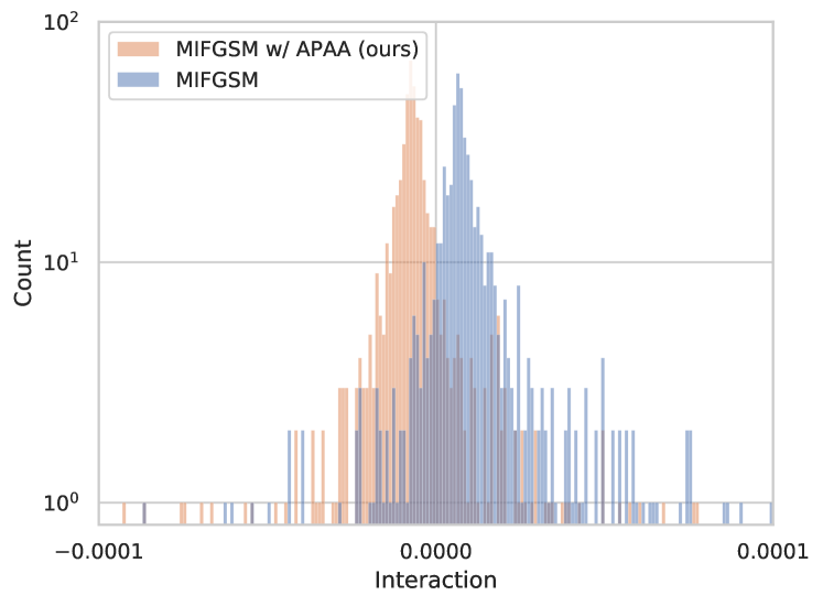
Figure 3: The comparison of histograms of the interaction inside perturbations generated by our APAA and that of MIFGSM [11]. Smaller interaction values correspond to better black-box transferability. The experiment is conducted on 1000 images of CIFAR10 testset.

Moreover, we also verify our proof by experiments. As shown in Fig. 3, we can clearly see that the interaction inside perturbations generated by our APAA is significantly smaller than that of MIFGSM. Combined with the negative correlation between the adversarial transferability and the interaction inside adversarial perturbations, our proposed APAA method is theoretically proven to have better black-box transferability.

4 Experiments

We first introduce the setting of experiments in Sec. 4.1. Then we demonstrate the effectiveness of our proposed APAA with fixed scaling factor in Sec. 4.2. Finally, we conduct several experiments to show the superiority of the adaptive scaling factor generator in Sec. 4.3. We denote the APAA with the fixed scaling factor as $\text{APAA}_{f}$ and the APAA with the adaptive scaling factor generator as $\text{APAA}_{a}$.

4.1 Experiment Setting

Datasets. We use ImageNet [39] and CIFAR10 [40] datasets to conduct the experiments. CIFAR10 has 50000 training images and 10000 test images in different classes. For ImageNet, we use two sets of subsets^, in the ImageNet dataset [39] to conduct experiments. Each set contains 1000 images, covering almost all categories in ImageNet, which has been widely used in previous works. The maximation perturbation budgets on CIFAR10 and ImageNet are 8 and 16 with $L_{\infty}$ norm under the scale of 0-255, respectively.

Evaluation Models. We use both normally trained models and defense models to evaluate all attack methods. For CIFAR10, we use totally 8 normally trained models and 7 defense models for comprehensive evaluations. For ImageNet, we use totally 9 normally trained models and 12 defense models to evaluate. Specifically, the models used for CIFAR10 includes RegNet [41], Res-18 [42], SENet-18 [43], Dense-121 [44], WideRes_28$\times$10 [45], DPN [46], Pyramid [47], ShakeShake [48], Dense-121_adv [10], GoogLeNet_adv [10], Res-18_adv [10], $k$-WTA [49], Odds [50], Generative [51] and Ensemble [31]. The models used for ImageNet include IncRes-v2 [52], Inc-v3 [53], Inc-v4 [52], Res-101 [54], Res-152 [54], Mob_1.0 [55], Mob_1.4 [55], PNAS [56], NAS [57], Inc-v3_adv [21], Inc-v3_ens3 [21], Inc-v3_ens4 [21], IncRes-v2_ens [21], HGD [26], R&P [58], NIPS-r3, Bit-Red [59], JPEG [60], FD [28], ComDefend [29] and RS [36].

Metrics. We use the attack success rates on both white-box and black-box models to evaluation the effectiveness of different methods. Since all methods constrain the same $L_{\infty}$ perturbation budget, we additionally use mean absolute distance (MAD) and root mean square distance (RMSD) to compare the magnitude of perturbations generated by different methods.

TABLE I: The hyperparameters used in baseline methods on ImageNet and CIFAR10 datasets. For the dataset of ImageNet, we use the hyperparameters reported in origin papers. For the dataset of CIFAR10, we find that the setting used in ImageNet is ineffective and determine the optimal value by hyperparameter searching.

	ImageNet	CIFAR10
MIFGSM	$\mu=1.0$	$\mu=1.0$
DIM	$p=0.7$	$p=0.7$
TIM	$k=15$	$k=3$
SIM	$m=5$	$m=2$
VT	$N=20$, $\beta=1.5$
EMI	$N=11$, $\eta=7$
SGM	$\gamma=0.2$ for Res-152, $\gamma=0.5$ for Dense-201
IR	$\lambda=1$ for Res-34, $\lambda=2$ for Dense-121
AIFGTM	$\lambda=1.3$, $\mu_{1}=1.5$, $\mu_{2}=1.9$, $\beta_{1}=0.9$, $\beta_{2}=0.99$

Baselines. We use MIFGSM [11], DIM [12], TIM [13], SIM [14], VT [18], EMI [19], AIFGTM [20], SGM [17] and IR [15] as baselines to compare with our proposed method. The details of the hyperparameters in these methods are provided in Tab. I. The number of iteration $T$ in the generation of adversarial examples for all methods, including ours, is 10 unless mentioned. We clip the adversarial examples to the range of the normal image (i.e., 0-255) and constrain the adversarial perturbations within the perturbation budget on $L_{\infty}$ norm bound in each step of the iteration process.

Details. For the method of fixed scaling factor, we select 10000 training images of CIFAR10 and one subset of ImageNet¹ as the validation set to search for the best scaling factor, and utilize the corresponding scaling factor to conduct the attack and evaluation in the testset of CIFAR10 and the other subset of ImageNet², respectively. By searching on the validation set, we set the scaling factor $\gamma$ as 8 for all methods on CIFAR10. For ImageNet, we use 0.4 in TIM, EMI, SGM, IR, and 0.8 in VT and AIFGTM as the scaling factor $\gamma$. We train the adaptive scaling factor generator with the training set of CIFAR10. The training of the model is quite fast. It takes about 2-3 hours on a GTX 1080Ti GPUs with 3-4 epochs. The architecture of the generator is shown in Tab. II. It should be mentioned that our proposed generator needs at least two white-box models to train. Through experiments, we find that when training the generator with only one classifier model, i.e., $n=1$ and $C_{x}=C_{y}$, the generated scaling factor is as high as possible. Although the higher white-box attack success rate can be achieved in this case, the transferability of generated adversarial examples is dropped dramatically. To maintain the transferability of adversarial examples, we use different classifier models when calculating the gradient information and updating the parameters of generator $G_{t}$, so that the generated scaling factor will not overfit to a specific model.

TABLE II: The architecture of the adaptive scaling factor generator. The $k$, $s$ and $p$ in the Conv2d layer means the kernel size, stride and padding, respectively.

No.	Layer	Input Shape	Output Shape
1	Conv2d(k=3, s=2, p=1)	[32,32,6]	[16,16,32]
2	InstanceNorm2d	[16,16,32]	[16,16,32]
3	Conv2d(k=3, s=2, p=1)	[16,16,32]	[8,8,32]
4	InstanceNorm2d	[8,8,32]	[8,8,32]
5	Conv2d(k=3, s=2, p=1)	[8,8,32]	[4,4,32]
6	InstanceNorm2d	[4,4,32]	[4,4,32]
7	Flatten	[4,4,32]	[512]
8	Linear	[512]	[128]
9	Linear	[128]	[1]

4.2 Attack with Fixed Scaling Factor

We conduct comprehensive experiments on CIFAR10 and ImageNet to demonstrate the effectiveness of our proposed $\text{APAA}_{f}$, i.e., replacing the sign normalization with a fixed scaling factor. The value of the scaling factor in the experiments is determined by manually hyperparameter searching within a certain range on the validation set, which is totally separate from the test set used in the experiments below.

TABLE III: The attack success rates of the adversarial examples on CIFAR10 under untargeted attack setting.

(a) The evaluation on the normally trained models.

Source Model	Method	Target Model								Distance Metric
		RegNet	Res-18	SENet-18	Dense-121	WideRes28$\times$10	DPN	Pyramid	ShakeShake	MAD	RMSD
RegNet	MIFGSM [11]	99.1	88.8	88.8	90.2	84.6	86.1	79.3	83.1	5.470	5.841
	MIFGSM w/ APAAf	99.8	92.7	92.3	93.8	88.8	89.9	82.4	87.1	5.377	5.754
	DIM [12]	98.0	91.0	90.7	91.8	88.2	88.2	85.1	86.6	5.544	5.892
	DIM w/ APAAf	99.4	94.9	94.6	95.5	92.5	92.3	89.2	91.3	5.309	5.682
	SIM [14]	98.1	93.2	93.2	94.0	91.5	90.6	88.2	89.6	5.606	5.949
	SIM w/ APAAf	99.4	96.5	96.4	97.1	95.6	94.4	92.7	93.5	5.343	5.708
RegNet +Res-18 +SENet-18 +Dense-121	MIFGSM [11]	98.0	98.5	99.5	99.0	96.1	94.5	94.2	95.4	5.636	5.984
	MIFGSM w/ APAAf	99.4	99.6	100.0	99.9	98.7	97.8	97.5	98.2	5.496	5.856
	DIM [12]	97.6	98.4	99.3	98.7	96.6	94.7	94.8	95.9	5.688	6.017
	DIM w/ APAAf	99.4	99.7	99.9	99.7	98.7	97.6	97.9	98.5	5.427	5.783
	SIM [14]	97.8	98.6	99.4	98.9	97.3	95.6	95.7	96.6	5.747	6.065
	SIM w/ APAAf	99.3	99.7	99.9	99.8	99.3	98.1	98.3	98.8	5.462	5.807

(b) The evaluation on the defense models.

Source Model	Method	Target Model
		Dense-121adv	GoogLeNetadv	Res-18adv	$k$-WTA	Odds	Generative	Ensemble
RegNet	MIFGSM [11]	21.0	45.1	15.9	75.5	87.0	53.6	79.7
	MIFGSM w/ APAAf	23.3	50.0	18.8	78.6	91.4	55.7	83.0
	DIM [12]	23.4	53.5	17.9	80.1	90.8	59.9	84.2
	DIM w/ APAAf	30.6	61.6	23.8	84.5	94.7	62.1	88.5
	SIM [14]	25.0	57.5	18.8	84.5	93.6	63.0	87.9
	SIM w/ APAAf	31.7	64.7	23.8	88.6	96.8	65.1	92.1
RegNet +Res-18 +SENet-18 +Dense-121	MIFGSM [11]	34.6	69.5	25.6	92.1	97.5	72.2	93.2
	MIFGSM w/ APAAf	38.9	73.5	30.8	95.8	99.5	74.9	96.8
	DIM [12]	36.4	71.8	27.2	92.7	98.4	74.1	94.1
	DIM w/ APAAf	38.9	73.5	30.8	95.8	99.5	74.9	96.8
	SIM [14]	39.0	73.9	28.4	94.0	99.0	75.4	95.2
	SIM w/ APAAf	45.5	79.5	35.3	97.3	99.7	78.1	97.7

TABLE IV: The attack success rates of the adversarial examples on ImageNet under untargeted attack setting.

(a) The evaluation on the normally trained models.

Source Model	Method	Target Model									Distance Metric
		IncRes-v2	Inc-v3	Inc-v4	Res-101	Res-152	Mob1.0	Mob1.4	PNAS	NAS	MAD	RMSD
IncRes-v2	TIM [13]	98.3	86.5	83.9	73.3	73.8	81.4	83.7	75.1	77.3	10.302	11.108
	TIM w/ APAAf	98.6	88.6	85.4	75.3	76.1	83.7	87.9	77.2	80.2	8.887	9.693
	VT [18]	98.5	89.1	87.0	79.8	80.4	82.6	86.6	80.5	82.2	10.031	10.810
	VT w/ APAAf	99.5	92.3	90.9	82.6	82.9	87.5	90.6	83.8	85.4	9.513	10.299
	EMI [19]	99.5	95.1	93.0	88.0	87.3	90.8	93.8	89.8	92.0	10.479	11.283
	EMI w/ APAAf	99.6	97.0	95.9	90.2	90.5	93.6	95.2	91.8	92.7	9.390	10.234
	AIFGTM [20]	97.4	82.2	78.0	72.5	72.4	77.1	80.4	74.0	75.1	10.415	11.269
	AIFGTM w/ APAAf	98.3	84.2	81.8	74.2	74.0	80.5	84.5	78.2	79.7	9.004	9.742
IncRes-v2 +Inc-v3 +Inc-v4 +Res-101	TIM [13]	98.5	99.4	99.0	97.0	93.0	92.8	94.3	91.8	93.5	10.289	11.155
	TIM w/ APAAf	99.7	99.9	99.7	99.0	97.6	95.9	98.2	95.5	96.5	9.019	9.898
	VT [18]	94.8	99.5	97.0	90.3	90.5	91.8	93.4	90.5	91.0	9.717	10.565
	VT w/ APAAf	98.3	99.7	98.8	95.5	94.9	95.1	96.4	94.6	95.5	9.417	10.257
	EMI [19]	99.4	99.9	99.6	98.2	97.1	97.5	98.3	97.1	97.7	10.557	11.391
	EMI w/ APAAf	99.7	100.0	99.8	99.0	98.3	99.1	99.3	98.6	98.5	9.489	10.381
	AIFGTM [20]	98.0	98.9	98.5	96.2	91.7	90.7	94.1	90.3	91.7	10.475	11.378
	AIFGTM w/ APAAf	98.6	99.4	99.1	97.6	94.5	93.7	96.0	93.5	94.0	9.070	9.865

(b) The evaluation on the defense models.

Source Model	Method	Target Model
		Inc-v3adv	Inc-v3ens3	Inc-v3ens4	IncRes-v2ens	HGD	R&P	NIPS-r3	Bit-Red	JPEG	FD	ComDefend	RS
IncRes-v2	TIM [13]	56.4	64.7	55.7	51.6	60.6	53.0	59.1	42.4	75.3	67.2	70.3	36.2
	TIM w/ APAAf	68.2	66.2	60.3	54.0	62.2	54.9	61.0	43.9	76.6	69.7	71.3	40.5
	VT [18]	69.4	73.8	70.3	69.0	71.7	67.5	71.1	50.6	80.2	74.2	77.1	44.1
	VT w/ APAAf	79.2	77.5	72.3	70.1	74.7	68.7	72.3	52.5	83.6	76.2	79.9	46.6
	EMI [19]	76.8	79.3	71.3	66.2	76.9	69.1	76.0	58.9	87.8	83.3	84.9	50.2
	EMI w/ APAAf	86.5	83.7	76.3	74.6	80.2	75.2	79.1	60.9	90.3	85.3	87.5	56.9
	AIFGTM [20]	68.7	68.1	61.1	63.1	64.9	62.2	64.2	44.3	71.8	67.4	67.6	38.9
	AIFGTM w/ APAAf	72.2	70.5	65.9	63.4	67.4	62.6	65.6	46.1	75.5	71.7	73.1	45.8
IncRes-v2 +Inc-v3 +Inc-v4 +Res-101	TIM [13]	85.2	86.7	85.3	78.3	86.6	79.9	84.3	62.9	91.4	83.6	88.4	56.2
	TIM w/ APAAf	92.8	91.1	90.0	83.0	91.5	85.7	89.0	65.0	94.1	87.5	90.9	61.1
	VT [18]	85.1	85.4	83.8	79.1	83.6	79.3	82.3	66.7	88.8	84.1	86.6	60.8
	VT w/ APAAf	93.6	93.1	91.5	86.0	91.6	87.2	89.6	73.4	95.0	88.4	92.7	69.0
	EMI [19]	92.5	91.4	89.5	84.4	91.2	85.6	89.6	75.6	95.9	91.6	94.3	68.8
	EMI w/ APAAf	96.6	95.6	93.9	89.4	95.1	91.0	92.7	78.8	97.2	93.6	95.5	73.0
	AIFGTM [20]	88.7	88.0	86.1	81.4	86.8	81.9	84.5	63.4	88.7	82.0	85.5	57.3
	AIFGTM w/ APAAf	92.6	91.1	89.7	86.7	92.1	87.2	89.3	69.1	93.0	86.3	90.7	65.6

TABLE V: The attack success rates of SGM [17] and our APAA_f method on ImageNet under untargeted attack setting.

(a) The evaluation on the normally trained models.

Source Model	Method	Target Model									Distance Metric
		Dense-201	Res-152	Res-34	VGG-16	VGG-19	SENet-154	Inc-v3	Inc-v4	IncRes-v2	MAD	RMSD
Dense-201	SGM [17]	100.0	94.9	94.6	90.1	90.2	86.5	84.6	80.4	79.1	9.947	10.805
	SGM w/ APAAf	100.0	95.7	95.9	92.1	90.8	88.5	85.4	82.7	81.5	9.694	10.528
Res-152	SGM [17]	87.4	99.9	92.7	89.9	88.1	77.6	79.6	74.3	72.9	10.089	10.988
	SGM w/ APAAf	87.8	99.9	93.5	91.9	89.4	78.7	81.8	75.5	75.8	9.487	10.357

(b) The evaluation on the defense models.

Source Model	Method	Target Model
		Inc-v3adv	Inc-v3ens3	Inc-v3ens4	IncRes-v2ens	HGD	R&P	NIPS-r3	Bit-Red	JPEG	FD	ComDefend	RS
Dense-201	SGM [17]	71.8	66.6	67.4	58.2	79.4	58.1	64.6	48.6	71.2	65.6	58.0	53.0
	SGM w/ APAAf	75.6	70.1	69.8	60.4	82.7	62.4	67.4	51.3	73.2	66.3	60.1	54.7
Res-152	SGM [17]	62.8	57.8	55.5	46.1	76.4	47.2	52.0	43.4	62.8	57.2	47.6	42.0
	SGM w/ APAAf	65.8	62.0	58.1	48.6	77.0	51.2	54.5	45.4	66.7	60.3	48.9	43.0

TABLE VI: The attack success rates of IR [15] and our APAA_f method on ImageNet under untargeted attack setting. The results of the IR method are the results reported in their paper.

Source Model	Method	Target Model
		Res-34	Dense-121	VGG-16	Res-152	Dense-201	SENet-154	Inc-v3	Inc-v4	IncRes-v2
Res-34	IR [15]	-	-	90.0	85.7	88.5	67.0	66.9	60.2	53.9
	IR w/ APAAf	97.7	92.0	90.6	88.5	90.0	72.2	68.5	63.3	59.8
Dense-121	IR [15]	-	-	89.0	83.2	93.4	74.2	69.6	64.7	58.2
	IR w/ APAAf	89.8	98.1	89.7	87.7	96.2	78.9	73.3	70.0	66.5

The untargeted attack. The experiments of adversarial examples generated on CIFAR10 and ImageNet under the untargeted attack setting are shown in Tab. III and Tab. IV respectively. From the results on both the single model and the ensembled model attacks, combined with our proposed method of the scaling factor, the attack success rates of generated adversarial examples in all the state-of-the-art methods are improved. In addition, under the same perturbation budget constrain on $L_{\infty}$ norm, the MAD and RMSD between the original images and generated adversarial examples of our $\text{APAA}_{f}$ are smaller than the existing methods. Due to the accurate gradient directions used in our proposed method, our attack method is more effective, which has higher attack success rates with fewer perturbations. We also conduct experiments on SGM [17] and IR [15] methods in Tab. V and Tab. VI, respectively. It demonstrates that our method can well integrate with almost all gradient-based attack methods to improve the attack success rates.

TABLE VII: The attack success rates of the adversarial examples on CIFAR10 under targeted attack setting.

Source Model	Method	Target Model								Distance Metric
		RegNet	Res-18	SENet-18	Dense-121	WideRes28$\times$10	DPN	Pyramid	ShakeShake	MAD	RMSD
RegNet	MIFGSM [11]	82.6	44.7	44.1	46.3	39.9	42.8	36.7	40.2	5.363	5.734
	MIFGSM w/ APAAf	90.5	53.6	52.4	54.5	46.8	50.5	42.9	47.7	5.206	5.585
	DIM [12]	71.2	45.4	45.0	46.5	41.5	43.0	39.7	41.9	5.436	5.790
	DIM w/ APAAf	80.6	54.8	53.1	55.8	50.5	51.3	47.9	51.0	5.147	5.523
	SIM [14]	75.0	50.6	50.2	52.4	48.1	48.1	44.8	47.7	5.488	5.837
	SIM w/ APAAf	84.4	61.2	60.0	62.5	58.2	57.2	54.1	56.8	5.168	5.537
RegNet +Res-18 +SENet-18 +Dense-121	MIFGSM [11]	77.8	82.1	87.6	85.7	70.2	65.0	65.6	69.9	5.513	5.865
	MIFGSM w/ APAAf	89.0	91.9	94.9	93.7	82.8	76.6	76.8	82.2	5.365	5.729
	DIM [12]	73.5	78.8	83.9	80.8	69.3	62.8	65.3	69.3	5.552	5.889
	DIM w/ APAAf	84.8	88.8	92.0	90.1	81.1	74.4	76.7	80.8	5.289	5.650
	SIM [14]	75.8	81.6	86.2	83.7	73.1	65.7	68.5	72.7	5.582	5.911
	SIM w/ APAAf	87.1	91.0	93.8	92.3	84.7	77.2	79.5	83.5	5.279	5.632

The targeted attack. The experiments of adversarial examples generated on CIFAR10 under the targeted attack setting are shown in Tab. VII. The target label of each image is randomly chosen among the 9 wrong labels. The average black-box attack success rates of the adversarial examples generated by $\text{APAA}_{f}$ against white-box and black-box models are about 10% higher than those of baselines under both settings of the single model attack and the ensembled model attack. It verifies that our proposed scaling factor method is also effective under the targeted attack setting.

The size of perturbation.

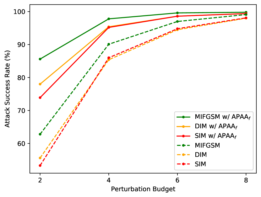
(a) White-box model

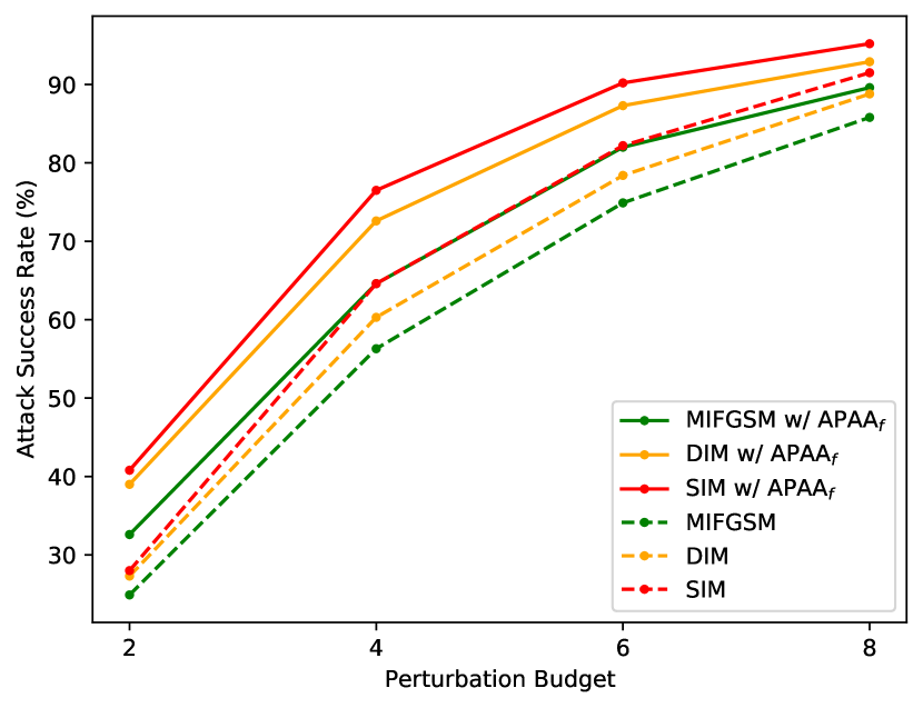
(b) Black-box normally trained model

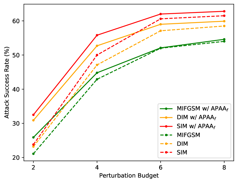
(c) Defense model

Figure 4: The attack success rates vs. perturbation budget curve on CIFAR10. The curves with dotted lines are the results of baseline methods, and those with solid lines are the results of our method. Three subfigures are the average attack success rates of different methods on the white-box model, the black-box normally trained models and the defense models, respectively. The experiment chooses RegNet as the white-box model.

We conduct experiments to demonstrate the attack success rates vs. perturbation budget curves on CIFAR10 in Fig. 4. We can clearly find that our proposed method of using the scaling factor improves the attack success rates on various perturbation budgets, which shows the excellent generalization of our method.

TABLE VIII: The attack success rates of the adversarial examples on CIFAR10 under untargeted attack setting with different number of iterations.

Source Model	Method	Target Model
		RegNet	Res-18	SENet-18	Dense-121	DPN	ShakeShake	Denseadv	GoogLeNetadv	Res-18adv	$k$-WTA	Ensemble
Res-18 +Dense-121	SIM [14] (8 steps)	94.0	98.4	96.8	98.9	91.7	94.2	20.5	53.8	19.9	90.4	92.1
	SIM [14] (10 steps)	96.4	99.3	98.2	99.5	94.4	96.3	23.9	55.9	20.7	92.8	94.4
	SIM w/ APAAf (8 steps)	96.7	99.5	98.7	99.7	94.5	97.0	31.5	64.7	26.8	93.1	94.6
	SIM w/ APAAf (10 steps)	97.9	99.7	99.2	99.9	95.6	97.8	32.5	65.3	27.2	93.7	95.3

The number of iteration steps. From Tab. VIII, we can see that under the same number of iteration steps, our $\text{APAA}_{f}$ consistently achieves higher attack success rates than SIM [14] method. It is worth mentioning that the result obtained by our $\text{APAA}_{f}$ with 8 steps attack is even better than the result of the SIM method with 10 steps. And on this basis, our $\text{APAA}_{f}$ with 10 steps can further improve the attack success rate. It confirms our opinion that accurate gradient directions can conduct a successful attack with fewer attack steps.

The visualization of adversarial examples.

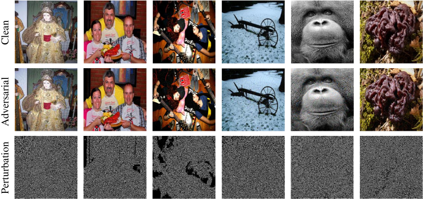
Figure 5: Visualization of adversarial examples crafted on IncRes-v2 by MIFGSM [11] with our proposed APAA_f.

We provide a visualization of our generated adversarial examples. As shown in Fig. 5, since our method can conduct the attack with relatively fewer perturbations, the generated adversarial perturbations are almost imperceptible.

4.3 Attack with Adaptive Scaling Factor

Algorithm 2 Generating adversarial examples with adaptive scaling factor generator

1:the original image $x$ and corresponding label $y$

2:the number of attack iteration $T$

3:the scaling factor generators $G_{1},G_{2},\cdots,G_{T}$

4:the ensembled model $C$, which contains all white-box classifier models $C_{1},\cdots,C_{n}$

5:the adversarial example $x_{T}^{adv}$

6:$x_{0}^{adv}=x$

7:for t $\in\{1,\cdots T\}$  do

8:     $grad_{t}=\nabla_{x}J(C(x_{t-1}^{adv}),y)$

9:     $\gamma_{t}=G_{t}(x_{t-1}^{adv},grad_{t})$

10:     $x_{t}^{adv}=\Pi_{x,\epsilon}(\gamma_{t}\cdot grad_{t}+x_{t-1}^{adv})$ $\triangleright$ using the update in BIM as an example

11:end for

12:return $x_{T}^{adv}$

TABLE IX: The comparisons between the attack success rates of the adversarial examples by SIM, our proposed method with fixed scaling factor and our proposed method with adaptive scaling factor against both normally trained models and defense models on CIFAR10 under untargeted attack setting.

Source Model	Method	Target Model										Distance Metric
		RegNet	Res-18	SENet-18	DPN	ShakeShake	Dense-121adv	GoogLeNetadv	Res-18adv	$k$-WTA	Ensemble	MAD	RMSD
Res-18 +GoogLeNetadv	SIM [14]	95.4	99.0	97.3	92.8	95.5	49.4	97.5	30.1	91.8	94.1	5.789	6.401
	SIM w/ APAAf	96.7	99.5	98.5	94.5	96.9	54.7	98.7	33.6	93.0	95.3	5.158	5.893
	SIM w/ APAAa	96.9	99.6	98.7	94.8	97.3	54.7	99.0	33.7	93.4	95.4	5.151	5.891
Res-18 +SENet-18 +Dense-121adv +GoogLeNetadv	SIM [14]	96.9	98.8	99.5	95.5	97.1	89.7	95.8	38.8	94.6	96.1	5.891	6.477
	SIM w/ APAAf	98.1	99.5	99.8	96.9	98.2	92.5	97.8	41.6	96.1	97.5	5.202	5.942
	SIM w/ APAAa	98.0	99.5	99.8	96.8	98.4	92.5	97.9	45.9	95.8	97.1	4.896	5.687

We further demonstrate the effectiveness of our proposed adaptive scaling factor generator. The process of generating adversarial examples with $\text{APAA}_{a}$ is summarized in Algorithm 2. For fair comparisons, we consider all the models used during the training of the generator ($C_{1},\cdots,C_{n}$) as white-box models, and conduct both attacks of SIM and our method on the ensemble of all white-box models. As shown in Tab. IX, when using the scaling factor generated by the generator proposed in Sec. 3.2.2 to generate the adversarial examples, it achieves comparative or even higher attack success rates, which saves the trouble of manually searching for the best hyperparameter of scaling factor. The means of the scaling factor generated under the two models ensembled and four models ensembled settting are 8.38 and 7.74, respectively, which is near the best manually selected hyperparameter (i.e., $\gamma$=8). Moreover, the standard deviations are 4.47 and 4.82, respectively. It demonstrates that the generator can adaptively generate different scaling factors with a certain diversity in different steps according to the characteristics of images.

5 Conclusion

In this work, we propose to use the scaling factor instead of the sign function to normalize the gradient of the input example when conducting the adversarial attack, which can achieve a more accurate gradient direction and thus improve the attack success rate. The scaling factor can either be elaborately selected manually, or adaptively achieved by a generator according to different image characteristics. We also theoretically demonstrate that our proposed method can improve the black-box transferability of adversarial examples. Extensive experiments on CIFAR10 and ImageNet show the superiority of our proposed methods, which can improve the black-box attack success rates on both normally trained models and defense models with fewer update steps and perturbation budgets.

Zheng Yuan received the B.S. degree from University of Chinese Academy of Sciences in 2019. He is currently pursuing the Ph.D. degree from University of Chinese Academy of Sciences. His research interest includes adversarial example and model robustness. He has authored several academic papers in international conferences including ICCV/ECCV/ICPR.

Jie Zhang is an associate professor with the Institute of Computing Technology, Chinese Academy of Sciences (CAS). He received the Ph.D. degree from the University of Chinese Academy of Sciences, Beijing, China. His research interests cover computer vision, pattern recognition, machine learning, particularly include face recognition, image segmentation, weakly/semi-supervised learning, domain generalization.

Zhaoyan Jiang received the MS degree in Pattern Recognition and Intelligent System from Northeastern University in 2013. He currently works as a research engineer in Tencent, Inc, Beijing, China. His research interests include computer vision, metric learning and image processing.

Liangliang Li received the MS degree in Computer Science and Technology from Tsinghua University in 2018. He currently works as a research engineer in Tencent, Inc, Beijing, China. His research interests include computer vision, metric learning and image processing.

Shiguang Shan received Ph.D. degree in computer science from the Institute of Computing Technology (ICT), Chinese Academy of Sciences (CAS), Beijing, China, in 2004. He has been a full Professor of this institute since 2010 and now the deputy director of CAS Key Lab of Intelligent Information Processing. His research interests cover computer vision, pattern recognition, and machine learning. He has published more than 300 papers, with totally more than 29,000 Google scholar citations. He has served as Area Chair (or Senior PC) for many international conferences including ICCV11, ICPR12/14/20, ACCV12/16/18, FG13/18, ICASSP14, BTAS18, AAAI20/21, IJCAI21, and CVPR19/20/21. And he was/is Associate Editors of several journals including IEEE T-IP, Neurocomputing, CVIU, and PRL. He was a recipient of the China’s State Natural Science Award in 2015, and the China’s State S&T Progress Award in 2005 for his research work.

Appendix A Proof of Proposition 1

Proof.

We use mathematical induction to complete the proof. In the following proof, we use $g$ to denote the gradient $g(x)=\frac{\partial L(x)}{\partial x}$ and $H$ to denote the second-order Hessian matrix $H(x)$.

When $m=1$, from Eq. 17-Eq. 20, we get $a_{1}=1$, $b_{1}=0$, $c_{1}=1$, $d_{1}=0$. Taking these values into Eq. 15 and Eq. 16, we can get $g_{1}=g$, $\delta_{1}=\gamma g$, which satisfies the formula of MIFGSM [11] (i.e., Eq. 13 and Eq. 14).

Assuming that the proposition holds when $m=t$, when $m=t+1$,

$$g_{t+1}= \mu g_{t}+g(x+\delta_{t})$$ (22)

$$= \mu a_{t}g+\mu b_{t}\gamma gH+g+\delta_{t}H$$ (23)

$$= \mu a_{t}g+\mu b_{t}\gamma gH+g+(c_{t}\gamma gH+d_{t}\gamma^{2}gH)H$$ (24)

$$= (\mu a_{t}+1)g+(\mu b_{t}+c_{t})\gamma gH$$ (25)

where the second line is due to the first-order Taylor expansion, and we ignore second-order terms with respect to $H$ in forth line since $\|H\|\sim 0$.

$$\mu a_{t}+1$$

$$= \mu\sum_{i=1}^{t}\mu^{i-1}+1$$ (26)

$$= \sum_{i=1}^{t}\mu_{i}+1$$ (27)

$$= \sum_{i=1}^{t+1}\mu_{i-1}=a_{t+1}$$ (28)

$$\mu b_{t}+c_{t}$$

$$= \mu\sum_{i=1}^{t}(t-i+1)(i-1)\mu^{i-2}+\sum_{i=1}^{t}(t-i+1)\mu^{i-1}$$ (29)

$$= \sum_{i=1}^{t}(t-i+1)(i-1)\mu^{i-1}+\sum_{i=1}^{t}(t-i+1)\mu^{i-1}$$ (30)

$$= \sum_{i=1}^{t}(t-i+1)i\mu^{i-1}$$ (31)

$$= \sum_{i=2}^{t+1}(t-i+2)(i-1)\mu^{i-2}$$ (32)

$$= \sum_{i=1}^{t+1}(t-i+2)(i-1)\mu^{i-2}=b_{t+1}$$ (33)

So when $m=t+1$, Eq. 15 holds.

$$\delta_{t+1}= \delta_{t}+\gamma g_{t+1}$$ (34)

$$= c_{t}\gamma g+d_{t}\gamma^{2}gH+(\mu a_{t}+1)\gamma g+(\mu b_{t}+c_{t})\gamma^{2}gH$$ (35)

$$= (\mu a_{t}+c_{t}+1)\gamma g+(\mu b_{t}+c_{t}+d_{t})\gamma^{2}gH$$ (36)

$$\mu a_{t}+c_{t}+1$$

$$= \mu\sum_{i=1}^{t}\mu^{i-1}+\sum_{i=1}^{t}(t-i+1)\mu^{i-1}+1$$ (37)

$$= \sum_{i=2}^{t+1}\mu^{i-1}+\sum_{i=1}^{t}(t-i+1)\mu^{i-1}+1$$ (38)

$$= \sum_{i=2}^{t}\mu^{i-1}+\sum_{i=2}^{t}(t-i+1)\mu^{i-1}+\mu^{t}+t+1$$ (39)

$$= \sum_{i=2}^{t}(t-i+2)\mu^{i-1}+\mu^{t}+t+1$$ (40)

$$= \sum_{i=1}^{t+1}(t-i+2)\mu^{i-1}=c_{t+1}$$ (41)

$$\mu b_{t}+c_{t}+d_{t}$$

$$= \mu\sum_{i=1}^{t}(t-i+1)(i-1)\mu^{i-2}+\sum_{i=1}^{t}(t-i+1)\mu^{i-1}$$

$$+\sum_{i=1}^{t}\frac{(t-i+2)(t-i+1)(i-1)}{2}\mu^{i-2}$$ (42)

$$= \sum_{i=1}^{t}(t-i+1)(i-1)\mu^{i-1}+\sum_{i=1}^{t}(t-i+1)\mu^{i-1}$$

$$+\sum_{i=1}^{t}\frac{(t-i+2)(t-i+1)(i-1)}{2}\mu^{i-2}$$ (43)

$$= \sum_{i=2}^{t+1}(t-i+2)(i-2)\mu^{i-2}+\sum_{i=2}^{t+1}(t-i+2)\mu^{i-2}$$

$$+\sum_{i=2}^{t+1}\frac{(t-i+2)(t-i+1)(i-1)}{2}\mu^{i-2}$$ (44)

$$= \sum_{i=2}^{t+1}(t-i+2)(i-2+1+\frac{(t-i+1)(i-1)}{2})\mu^{i-2}$$ (45)

$$= \sum_{i=2}^{t+1}\frac{(t-i+2)(t-i+3)(i-1)}{2}\mu^{i-2}$$ (46)

$$= \sum_{i=1}^{t+1}\frac{(t-i+2)(t-i+3)(i-1)}{2}\mu^{i-2}=d_{t+1}$$ (47)

So when $m=t+1$, Eq. 16 holds.

To sum up, we can get that when $m=t+1$, both Eq. 15 and Eq. 16 hold. Therefore, Proposition 1 is proved. ∎

Appendix B Proof of Proposition 2

Proof.

From the Lemma 1 in [15], the Shapley interaction between perturbation units $a,b$ can be written as $I_{ab}=\delta_{a}H_{ab}(x)\delta_{b}+\hat{R_{2}}(\delta)$, where $H_{ab}(x)=\frac{\partial L(x)}{\partial x_{a}\partial x_{b}}$ represents the element of the Hessian matrix, $\delta_{a}$ and $\delta_{b}$ are the $a$-th and $b$-th elements in $\delta$, $\hat{R_{2}}(\delta)$ denotes terms with elements in $\delta$ of higher than the second order. In the following proof, we ignore second-order terms of $\delta$ since $\|\delta\|\sim 0$. According to Proposition 1, the Shapley interaction between perturbation units $a,b$ in our proposed APAA can be further written as

$$I_{ab}= \delta_{a}H_{ab}\delta_{b}$$ (48)

$$= (c_{m}\gamma g_{a}+d_{m}\gamma^{2}gH_{*a})H_{ab}(c_{m}\gamma g_{b}+d_{m}\gamma^{2}gH_{*b})$$ (49)

$$= c_{m}^{2}\gamma^{2}g_{a}g_{b}H_{ab}+c_{m}d_{m}\gamma^{3}g_{b}H_{ab}gH_{*a}$$

$$+c_{m}d_{m}\gamma^{3}g_{a}H_{ab}gH_{*b}+O(H^{2}),$$ (50)

where $O(H^{2})$ is the second-order small quantity about $H$, which is ignored in the following calculations. We can further calculate the interaction inside perturbations generated by MIFGSM with APAA as follows

$$\mathbb{E}_{a,b}(I_{ab})= \mathbb{E}_{a,b}[c_{m}^{2}\gamma^{2}g_{a}g_{b}H_{ab}+c_{m}d_{m}\gamma^{3}g_{b}H_{ab}gH_{*a}$$

$$+c_{m}d_{m}\gamma^{3}g_{a}H_{ab}gH_{*b}]$$ (51)

$$= \gamma^{2}\mathbb{E}_{a,b}[c_{m}^{2}g_{a}g_{b}H_{ab}]+2\gamma^{3}\mathbb{E}_{a,b}[c_{m}d_{m}g_{a}H_{ab}gH_{*b}]$$ (52)

where $\mathbb{E}_{a,b}[c_{m}d_{m}g_{a}H_{ab}gH_{*b}]$ has been proven greater than 0 in Sec. E.2 in [15]. Therefore, the interaction inside adversarial perturbations generated by MIFGSM with APAA at $m$-th step is given as:

$$\mathbb{E}_{a,b}(I_{ab})=A\gamma^{2}+2B\gamma^{3},$$ (53)

where

$$A=\mathbb{E}_{a,b}[c_{m}^{2}g_{a}g_{b}H_{ab}],\quad B=\mathbb{E}_{a,b}[c_{m}d_{m}g_{a}H_{ab}gH_{*b}]\geq 0.$$

∎

References

- [1] C. Szegedy, W. Zaremba, I. Sutskever, J. Bruna, D. Erhan, I. J. Goodfellow, and R. Fergus, “Intriguing properties of neural networks,” in ICLR, 2014.
- [2] C. Xiao, B. Li, J. Zhu, W. He, M. Liu, and D. Song, “Generating adversarial examples with adversarial networks,” in IJCAI, 2018, pp. 3905–3911.
- [3] Z. Zhao, D. Dua, and S. Singh, “Generating natural adversarial examples,” in ICLR, 2018.
- [4] Y. Song, R. Shu, N. Kushman, and S. Ermon, “Constructing unrestricted adversarial examples with generative models,” in NeurIPS, 2018, pp. 8322–8333.
- [5] A. Joshi, A. Mukherjee, S. Sarkar, and C. Hegde, “Semantic adversarial attacks: Parametric transformations that fool deep classifiers,” in ICCV, 2019, pp. 4772–4782.
- [6] H. Qiu, C. Xiao, L. Yang, X. Yan, H. Lee, and B. Li, “Semanticadv: Generating adversarial examples via attribute-conditioned image editing,” in ECCV, 2020, pp. 19–37.
- [7] Z. Xiao, X. Gao, C. Fu, Y. Dong, W. Gao, X. Zhang, J. Zhou, and J. Zhu, “Improving transferability of adversarial patches on face recognition with generative models,” 2021, pp. 11 845–11 854.
- [8] I. J. Goodfellow, J. Shlens, and C. Szegedy, “Explaining and harnessing adversarial examples,” in ICLR, 2015.
- [9] A. Kurakin, I. J. Goodfellow, and S. Bengio, “Adversarial machine learning at scale,” in ICLR, 2017.
- [10] A. Madry, A. Makelov, L. Schmidt, D. Tsipras, and A. Vladu, “Towards deep learning models resistant to adversarial attacks,” in ICLR, 2018.
- [11] Y. Dong, F. Liao, T. Pang, H. Su, J. Zhu, X. Hu, and J. Li, “Boosting adversarial attacks with momentum,” in CVPR, 2018, pp. 9185–9193.
- [12] C. Xie, Z. Zhang, Y. Zhou, S. Bai, J. Wang, Z. Ren, and A. L. Yuille, “Improving transferability of adversarial examples with input diversity,” in CVPR, 2019, pp. 2730–2739.
- [13] Y. Dong, T. Pang, H. Su, and J. Zhu, “Evading defenses to transferable adversarial examples by translation-invariant attacks,” in CVPR, 2019, pp. 4312–4321.
- [14] J. Lin, C. Song, K. He, L. Wang, and J. E. Hopcroft, “Nesterov accelerated gradient and scale invariance for adversarial attacks,” in ICLR, 2020.
- [15] X. Wang, J. Ren, S. Lin, X. Zhu, Y. Wang, and Q. Zhang, “A unified approach to interpreting and boosting adversarial transferability,” in ICLR, 2021.
- [16] Y. Nesterov, “A method for unconstrained convex minimization problem with the rate of convergence ,” 1983.
- [17] D. Wu, Y. Wang, S. Xia, J. Bailey, and X. Ma, “Skip connections matter: On the transferability of adversarial examples generated with resnets,” in ICLR, 2020.
- [18] X. Wang and K. He, “Enhancing the transferability of adversarial attacks through variance tuning,” in CVPR, 2021, pp. 1924–1933.
- [19] X. Wang, J. Lin, H. Hu, J. Wang, and K. He, “Boosting adversarial transferability through enhanced momentum,” arXiv preprint arXiv:2103.10609, 2021.
- [20] J. Zou, Z. Pan, J. Qiu, Y. Duan, X. Liu, and Y. Pan, “Making adversarial examples more transferable and indistinguishable,” arXiv preprint arXiv:2007.03838, 2020.
- [21] F. Tramèr, A. Kurakin, N. Papernot, I. J. Goodfellow, D. Boneh, and P. D. McDaniel, “Ensemble adversarial training: Attacks and defenses,” in ICLR, 2018.
- [22] C. Song, K. He, J. Lin, L. Wang, and J. E. Hopcroft, “Robust local features for improving the generalization of adversarial training,” in ICLR, 2020.
- [23] T. Pang, X. Yang, Y. Dong, T. Xu, J. Zhu, and H. Su, “Boosting adversarial training with hypersphere embedding,” in NeurIPS, 2020.
- [24] E. Wong, L. Rice, and J. Z. Kolter, “Fast is better than free: Revisiting adversarial training,” in ICLR, 2020.
- [25] G. K. Dziugaite, Z. Ghahramani, and D. M. Roy, “A study of the effect of jpg compression on adversarial images,” arXiv preprint arXiv:1608.00853, 2016.
- [26] F. Liao, M. Liang, Y. Dong, T. Pang, X. Hu, and J. Zhu, “Defense against adversarial attacks using high-level representation guided denoiser,” in CVPR, 2018, pp. 1778–1787.
- [27] P. Samangouei, M. Kabkab, and R. Chellappa, “Defense-gan: Protecting classifiers against adversarial attacks using generative models,” in ICLR, 2018.
- [28] Z. Liu, Q. Liu, T. Liu, N. Xu, X. Lin, Y. Wang, and W. Wen, “Feature distillation: Dnn-oriented JPEG compression against adversarial examples,” in CVPR, 2019, pp. 860–868.
- [29] X. Jia, X. Wei, X. Cao, and H. Foroosh, “Comdefend: An efficient image compression model to defend adversarial examples,” in CVPR, 2019, pp. 6084–6092.
- [30] X. Liu, M. Cheng, H. Zhang, and C. Hsieh, “Towards robust neural networks via random self-ensemble,” in ECCV, 2018, pp. 369–385.
- [31] T. Pang, K. Xu, C. Du, N. Chen, and J. Zhu, “Improving adversarial robustness via promoting ensemble diversity,” in ICML, 2019, pp. 4970–4979.
- [32] H. Yang, J. Zhang, H. Dong, N. Inkawhich, A. Gardner, A. Touchet, W. Wilkes, H. Berry, and H. Li, “DVERGE: diversifying vulnerabilities for enhanced robust generation of ensembles,” in NeurIPS, 2020.
- [33] A. Raghunathan, J. Steinhardt, and P. Liang, “Certified defenses against adversarial examples,” in ICLR, 2018.
- [34] E. Wong, F. R. Schmidt, J. H. Metzen, and J. Z. Kolter, “Scaling provable adversarial defenses,” in NeurIPS, 2018, pp. 8400–8409.
- [35] J. M. Cohen, E. Rosenfeld, and J. Z. Kolter, “Certified adversarial robustness via randomized smoothing,” in ICML, 2019, pp. 1310–1320.
- [36] J. Jia, X. Cao, B. Wang, and N. Z. Gong, “Certified robustness for top-k predictions against adversarial perturbations via randomized smoothing,” in ICLR, 2020.
- [37] M. Grabisch and M. Roubens, “An axiomatic approach to the concept of interaction among players in cooperative games,” Int. J. Game Theory, vol. 28, no. 4, pp. 547–565, 1999.
- [38] L. S. Shapley, A Value for n-Person Games, 1953, vol. 2, pp. 307–318.
- [39] O. Russakovsky, J. Deng, H. Su, J. Krause, S. Satheesh, S. Ma, Z. Huang, A. Karpathy, A. Khosla, M. S. Bernstein, A. C. Berg, and L. Fei-Fei, “Imagenet large scale visual recognition challenge,” IJCV, vol. 115, no. 3, pp. 211–252, 2015.
- [40] A. Krizhevsky, “Learning multiple layers of features from tiny images,” 2009.
- [41] I. Radosavovic, R. P. Kosaraju, R. B. Girshick, K. He, and P. Dollár, “Designing network design spaces,” in CVPR, 2020, pp. 10 428–10 436.
- [42] K. He, X. Zhang, S. Ren, and J. Sun, “Deep residual learning for image recognition,” in CVPR, 2016, pp. 770–778.
- [43] J. Hu, L. Shen, and G. Sun, “Squeeze-and-excitation networks,” in CVPR, 2018, pp. 7132–7141.
- [44] G. Huang, Z. Liu, L. van der Maaten, and K. Q. Weinberger, “Densely connected convolutional networks,” in CVPR, 2017, pp. 4700–4708.
- [45] S. Zagoruyko and N. Komodakis, “Wide residual networks,” arXiv preprint arXiv:1605.07146, 2016.
- [46] Y. Chen, J. Li, H. Xiao, X. Jin, S. Yan, and J. Feng, “Dual path networks,” in NeurIPS, 2017, pp. 4467–4475.
- [47] D. Han, J. Kim, and J. Kim, “Deep pyramidal residual networks,” in CVPR, 2017, pp. 5927–5935.
- [48] X. Gastaldi, “Shake-shake regularization,” arXiv preprint arXiv:1705.07485, 2017.
- [49] C. Xiao, P. Zhong, and C. Zheng, “Enhancing adversarial defense by k-winners-take-all,” in ICLR, 2020.
- [50] K. Roth, Y. Kilcher, and T. Hofmann, “The odds are odd: A statistical test for detecting adversarial examples,” in ICML, 2019, pp. 5498–5507.
- [51] Y. Li, J. Bradshaw, and Y. Sharma, “Are generative classifiers more robust to adversarial attacks?” in ICML. PMLR, 2019, pp. 3804–3814.
- [52] C. Szegedy, S. Ioffe, V. Vanhoucke, and A. A. Alemi, “Inception-v4, inception-resnet and the impact of residual connections on learning,” in AAAI, 2017, pp. 4278–4284.
- [53] C. Szegedy, V. Vanhoucke, S. Ioffe, J. Shlens, and Z. Wojna, “Rethinking the inception architecture for computer vision,” in CVPR, 2016, pp. 2818–2826.
- [54] K. He, X. Zhang, S. Ren, and J. Sun, “Identity mappings in deep residual networks,” in ECCV, 2016, pp. 630–645.
- [55] M. Sandler, A. G. Howard, M. Zhu, A. Zhmoginov, and L. Chen, “Mobilenetv2: Inverted residuals and linear bottlenecks,” in CVPR, 2018, pp. 4510–4520.
- [56] C. Liu, B. Zoph, M. Neumann, J. Shlens, W. Hua, L. Li, L. Fei-Fei, A. L. Yuille, J. Huang, and K. Murphy, “Progressive neural architecture search,” in ECCV, 2018, pp. 19–34.
- [57] B. Zoph, V. Vasudevan, J. Shlens, and Q. V. Le, “Learning transferable architectures for scalable image recognition,” in CVPR, 2018, pp. 8697–8710.
- [58] C. Xie, J. Wang, Z. Zhang, Z. Ren, and A. L. Yuille, “Mitigating adversarial effects through randomization,” in ICLR, 2018.
- [59] W. Xu, D. Evans, and Y. Qi, “Feature squeezing: Detecting adversarial examples in deep neural networks,” in NDSS, 2018.
- [60] C. Guo, M. Rana, M. Cissé, and L. van der Maaten, “Countering adversarial images using input transformations,” in ICLR, 2018.