Proper Elements for Space Debris

Abstract.

Proper elements are quasi-invariants of a Hamiltonian system, obtained through a normalization procedure. Proper elements have been successfully used to identify families of asteroids, sharing the same dynamical properties. We show that proper elements can also be used within space debris dynamics to identify groups of fragments associated to the same break-up event. The proposed method allows to reconstruct the evolutionary history and possibly to associate the fragments to a parent body.

The procedure relies on different steps: (i) the development of a model for an approximate, though accurate, description of the dynamics of the space debris; (ii) the construction of a normalization procedure to determine the proper elements; (iii) the production of fragments through a simulated break-up event.

We consider a model that includes the Keplerian part, an approximation of the geopotential, and the gravitational influence of Sun and Moon. We also evaluate the contribution of Solar radiation pressure and the effect of noise on the orbital elements. We implement a Lie series normalization procedure to compute the proper elements associated to semi-major axis, eccentricity and inclination. Based upon a wide range of samples, we conclude that the distribution of the proper elements in simulated break-up events (either collisions and explosions) shows an impressive connection with the dynamics observed immediately after the catastrophic event. The results are corroborated by a statistical data analysis based on the check of the Kolmogorov-Smirnov test and the computation of the Pearson correlation coefficient.

Keywords. Proper elements, Normal form, Space debris, Geopotential, Sun and Moon attractions, Solar radiation pressure, Noise, Statistical data analysis.

1. Introduction

Over the centuries perturbation theory has been used in different contexts of Celestial Mechanics, from the computation of the ephemerides of the Moon to the determination of the orbits of artificial satellites.

In the domain of nearly-integrable Hamiltonian systems, perturbation theory consists in a normalization procedure that implements a canonical change of coordinates so that the transformed system becomes integrable up to a remainder function. The integrable part of the transformed Hamiltonian admits integrals of motion, which are indeed quasi-integrals for the Hamiltonian system that includes the remainder. The normalization procedure is constructive in the sense that it allows us to determine the explicit expression of the new integrable part and, hence, of the quasi-integrals.

This procedure has been successfully used to compute the so-called proper elements, which are quasi-invariants of the dynamics, staying nearly constant over very long times. Proper elements found a striking application in the context of the grouping of asteroids to form families. We refer to [28] for a thorough review of the history of asteroid family identification. The idea at the basis of such computation is that objects with nearby proper elements might have been physically close in the past. One can even conjecture that such asteroids might be fragments of an ancestor parent body. Being obtained through the averaging method over short-period angles followed by a normal form procedure that averages out the long-period perturbations, proper elements retain the essential features of the original family formation, which can be lost when using the osculating elements at the present time.

Proper elements were used in 1918 by Hirayama ([22]), who noticed many asteroids with similar semi-major axes forming ring-shaped clusters in projections on the planes of non-singular equinoctial orbital elements; the radius of the ring represents a proper element. Later, Brouwer ([5]) computed proper elements using an improved theory of planetary motion, while Williams ([45]) developed a semianalytic theory of asteroid secular perturbations. Using Yuasa theory ([46]), Kozai identified asteroid families formed by high-inclination asteroids ([33], [35], [40]). Proper elements for celestial bodies in resonance, e.g. Trojan asteroids, were considered by Schubart ([43], see also [39]). A number of relevant works that included an extension of Yuasa theory were developed by Knežević and Milani (see, e.g., [37], [38], see also [34]). The latter authors widely discussed also an alternative method to compute the proper elements, based on a so-called synthetic theory, which uses a numerical integration, a digital filtering of the short-period terms and a Fourier analysis ([29], [30], [31], [32]).

Inspired by the results of the computation of proper elements for asteroids, in this work we aim at computing and testing proper elements for the space debris problem. The increasing number of space debris surrounding the Earth has become a serious threat for the safeguard of operative satellites and for space missions. Many efforts are concentrated to track and prevent catastrophic events involving space debris, which are normally hardly observable and have high velocities. Here, we develop a method to classify the space debris into families, such that one can recover useful information about their evolution.

The procedure can be split into the following main steps: (i) the development of a model that, in a given region, provides a good approximation of the dynamics of the space debris; (ii) using Lie series, the explicit construction of an iterative normalization procedure to determine the proper elements; (iii) the production of fragments through a simulated break-up event and their analysis by means of a comparison between initial osculating elements, mean elements after a given period of time, and proper elements computed using the mean elements.

We provide below some details of the above three steps.

1.1. The model

To study the dynamics around the Earth, it is convenient to split the region surrounding our planet into three main parts: Low-Earth-Orbits (LEO) between 90 and 2000 km of altitude, Medium-Earth-Orbits (MEO) between $2000$ and $30000$ km of altitude, Geosynchronous Earth’s Orbits (GEO) above $30000$ km of altitude (see Figure 1).

The motion in LEO-MEO-GEO is mainly governed by the gravitational field of the Earth, that must include also the fact that the shape of our planet is non spherical; in LEO it is important to consider the dissipative effect due to the atmospheric drag, while in MEO and GEO the gravitational influence of Moon and Sun, as well as the Solar radiation pressure (hereafter, SRP), play a very important role (see, e.g., [6], [11], [13], [21], [36], [42], [44]). We will limit our study to MEO and GEO, in which the dynamics is governed by a conservative model. The computation of quasi-invariants in GEO has been also approached in [7], [20].

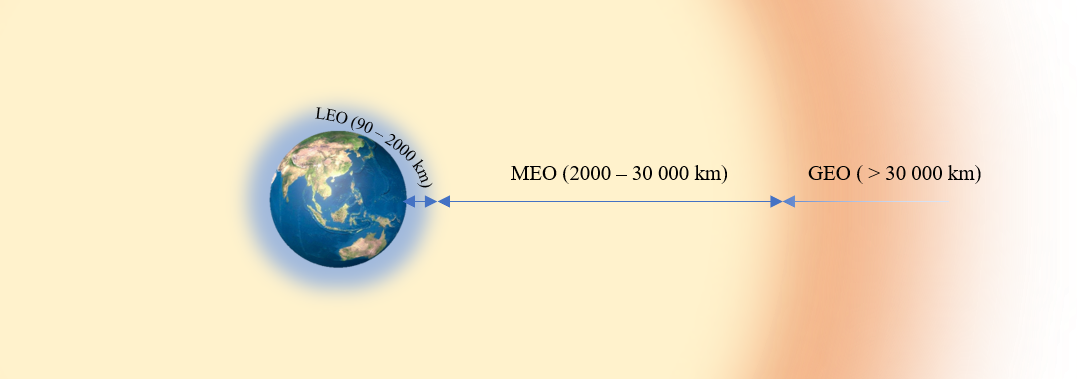
Figure 1. LEO: 90-2000 km, MEO: 2000-30000 km, GEO: $\geq$ 30000 km

In this work, we introduce a Hamiltonian function describing an approximation of the contribution of the sum of the Keplerian part, an expansion of the geopotential, and the gravitational influence of Moon and Sun. The resulting Hamiltonian depends upon the orbital elements of the debris, Moon, Sun and on the sidereal time accounting for the rotation of the Earth. Hence, the Hamiltonian depends upon a set of angular variables, that can be ordered hierarchically as fast, semi-fast and slow variables, since their rates change over days, months, years. We also investigate the effect of Solar radiation pressure, providing details on a specific sample.

The model is described in Section 2.

1.2. Normal forms

The normalization procedure is based upon the following strategy. We first average the model Hamiltonian over the fast and semi-fast angles; as a consequence of such averaging, the semi-major axis is constant and becomes the first proper element. As a result, we obtain a two degrees of freedom Hamiltonian, which depends on time, due to the variation of the longitude of the ascending node of the Moon. After the introduction of the extended Hamiltonian, we make an expansion around reference values of the action variables. Next, we proceed to implement a Lie series normalization to first order that allows us to determine two more proper elements, corresponding to eccentricity and inclination.

The normalization procedure is presented in Section 3.

1.3. Analysis of fragments’ clusters

To analyze groups of fragments originated from the same parent body, we use a simulator of break-up events based upon the program developed in [1]. We generate fragments from explosions or collisions of two satellites and we consider fragments with size greater than 12 cm. We consider break-up events occurring in three regions with different semi-major axis $a$: moderate altitude orbits ($a=15600$ km and $a=20600$ km), and medium altitude orbits ($a=33600$ km).

Our results consist in a comparison of the three sets of data providing semi-major axis, eccentricity and inclination, obtained as follows: we consider the elements just after break-up, after a propagation over 150 years, and we compute the proper elements based on the data propagated after 150 years. The results are presented in Section 4, which shows also some results obtained propagating the fragments to times less than 150 years. The distribution of the proper elements is analyzed by making the computations at different propagation times and this is supported by statistical data analysis by drawing histograms, by performing the Kolmogorov-Smirnov test and by computing the Pearson correlation coefficient.

This analysis is performed in non-resonant regions, but also resonant regions might be interesting as well. To this end, we introduce the definition of tesseral resonance, which corresponds to a commensurability involving the rate of variation of the mean anomaly of the debris and the rotation of the Earth. In Section 5, we extend the computation to the study of objects in the vicinity of resonant regions, precisely the 1:1 and 2:1 tesseral resonances. Finally, we complement the results by providing a sample in which we add the effect of noise to the initial mean elements.

From the results obtained in the non-resonant and resonant regions, we can draw the following conclusions: in several cases, the proper elements allow us to reconstruct a cluster structure, very similar to that which is formed just after the break-up. In particular, in the non-resonant case, the proper elements are an efficient tool to reconstruct the initial distribution. It is worth mentioning that some cases might be affected by lunisolar resonances ([4], [9], [10], [19], [23]) and therefore the cluster configuration can show anomalies in the distribution of the fragments.

The method presented in this paper represents an important tool for the classification of space debris into families; it is clear that such result has a major impact in many directions of paramount importance in space debris dynamics, most notably the identification of the space debris parent body.

Some further conclusions and perspectives of this work are given in Section 7.

2. The model

In this Section we introduce a model for the description of the dynamics of space debris, that takes into account four main contributions: the gravitational potential of the Earth, the attraction of the Moon, the attraction of the Sun, and the Solar radiation pressure. The model has been described in full detail in [7], [8], starting from the Cartesian equations of motion and using the expansion in orbital elements.

With reference to [7], [8], we consider a Hamiltonian function composed by the following parts:

$$\mathcal{H}=\mathcal{H}_{Kep}+\mathcal{H}_{E}+\mathcal{H}_{M}+\mathcal{H}_{S}+\mathcal{H}_{SRP}\ ,$$

where $\mathcal{H}_{Kep}$ denotes the Keplerian part due to the interaction with a spherical Earth, $\mathcal{H}_{E}$ is the contribution due to the non-spherical Earth, $\mathcal{H}_{M}$ and $\mathcal{H}_{S}$ denote, respectively, the Hamiltonian parts describing the attractions of Moon and Sun, $\mathcal{H}_{SRP}$ denotes the effect of Solar radiation pressure.

The Keplerian part takes a simple form, while the Hamiltonian functions $\mathcal{H}_{E}$, $\mathcal{H}_{M}$, $\mathcal{H}_{S}$, $\mathcal{H}_{SRP}$ have more complex expressions.

2.1. Keplerian Hamiltonian

The Keplerian Hamiltonian can be written in the form

$$\mathcal{H}_{Kep}(a)=-\frac{\mu_{E}}{2a}\ ,$$

where $a$ denotes the semi-major axis, $\mu_{E}=\mathcal{G}m_{E}$ with $\mathcal{G}$ the gravitational constant and $m_{E}$ the mass of the Earth.

2.2. Gravitational field of the Earth

Following [7], [8], [25], the Hamiltonian part corresponding to the geopotential perturbation - assuming that the Earth is not spherical - can be written as an expansion in the orbital elements $(a,e,i,M,\omega,\Omega)$ of the space object and depending on the sidereal time $\theta$, which takes into account the rotation of the Earth.

In a quasi-inertial reference frame (see Appendix A for more details), the Hamiltonian function can be written as

$$\mathcal{H}_{\text{E}}(a,e,i,M,\omega,\Omega,\theta)=-\frac{\mu_{E}}{a}\sum\limits^{\infty}_{n=2}\sum\limits^{n}_{m=0}(\frac{R_{E}}{a})^{n}\sum\limits^{n}_{p=0}F_{nmp}(i)\sum\limits^{\infty}_{q=-\infty}G_{npq}(e)S_{nmpq}(M,\omega,\Omega,\theta),$$ (2.1)

where $R_{E}$ is the Earth’s radius and the functions $F_{nmp}(i)$ and $G_{nmp}(e)$ are given by

$$F_{nmp}(i) = \sum\limits_{w=0}^{min(p,K)}\frac{(2n-2w)!}{w!(n-w)!(n-m-2w)!2^{2n-2w}}\sin^{n-m-2w}(i)\sum\limits^{m}_{s=0}{m\choose s}\cos^{s}(i)$$

$$\sum\limits^{n}_{c=0}{n-m-2w+s\choose c}{m-s\choose p-w-c}(-1)^{c-K}\ ,$$

$$G_{nmp}(e) = (-1)^{|q|}(1+\beta^{2})^{n}\beta^{|q|}\sum\limits_{k=0}^{\infty}P_{npqk}Q_{npqk}\beta^{2k}$$ (2.2)

with $K=[(n-m)/2]$ and $\beta$, $P_{npqk}$, $Q_{npqk}$ being functions of the eccentricity:

$$\beta = \frac{e}{1+\sqrt{1-e^{2}}}$$

$$P_{npqk} = \sum\limits_{r=0}^{h}{2p^{\prime}-2n\choose h-r}\frac{(-1)^{r}}{r!}\left(\frac{(n-2p^{\prime}+2q^{\prime})e}{2\beta}\right)^{r},\begin{cases}h=k+q^{\prime},q^{\prime}>0\\ h=k,q^{\prime}<0\end{cases}$$

$$Q_{npqk} = \sum\limits_{r=0}^{h}{-2p^{\prime}\choose h-r}\frac{1}{r!}\left(\frac{(n-2p^{\prime}+2q^{\prime})e}{2\beta}\right)^{r},\begin{cases}h=k,q^{\prime}>0\\ h=k-q^{\prime},q^{\prime}<0\ ,\end{cases}$$

while $p^{\prime}=p$ and $q^{\prime}=q$ when $p\leq n/2$, $p^{\prime}=n-p$ and $q^{\prime}=-q$ when $p>n/2$.

The quantity $S_{nmpq}$ in (2.1) is given by

$$S_{nmpq}=\begin{cases}-J_{nm}\cos(\Psi_{nmpq}),\qquad\mod(n-m,2)=0\\ -J_{nm}\sin(\Psi_{nmpq}),\qquad\mod(n-m,2)=1\ ,\end{cases}$$

where

$$\Psi_{nmpq}=(n-2p)\omega+(n-2p+q)M+m(\Omega-\theta)-m\lambda_{nm}$$ (2.3)

for some constants $\lambda_{nm}$, while $J_{nm}$ are related to the spherical harmonic coefficients of the geopotential ([26]). According to a standard notation, we define $J_{n}\equiv J_{n0}$. We remark that among the coefficients $J_{nm}$ of the Earth the biggest one is $J_{2}=-1.082\cdot 10^{-3}$; the values of the first few coefficients $J_{nm}$ and $\lambda_{nm}$ are listed in Table 1.

$n$	$m$	$J_{nm}$	$\lambda_{nm}$
2	0	$-1082.2626$	0
2	1	0.001807	$-81_{\cdot}^{\circ}5116$
2	2	1.81559	$75_{\cdot}^{\circ}0715$
3	0	$-2.53241$	0
3	1	2.20947	$186_{\cdot}^{\circ}9692$
3	2	0.37445	$72_{\cdot}^{\circ}8111$
3	3	0.22139	$80_{\cdot}^{\circ}9928$

Table 1. Values of $J_{nm}$ (in units of $10^{-6}$) and $\lambda_{nm}$ from [18].

Instead of the full expansion (2.1), we will consider only the secular part by averaging over the fast angles $M$ and $\theta$; this amounts to choose in (2.3) the terms with indexes $m=0$ and $n-2p+q=0$. The explicit expansions of $\mathcal{H}_{E}$ up to order $n=2$ or $n=3$, and including only the $J_{2}$ term, take the following form:

$$\mathcal{H}_{E}^{J_{2}}=\mu_{\text{E}}R_{\text{E}}^{2}J_{2}\frac{1+3\cos(2i)}{8a^{3}\left(1-e^{2}\right)^{3/2}},$$

while including both $J_{2}$ and $J_{3}$ terms, one obtains

$$\mathcal{H}_{E}^{J_{3}} = {{\mu_{\text{E}}R_{\text{E}}^{2}}\over a^{3}}\ J_{2}\ ({3\over 4}\sin^{2}i-{1\over 2}){1\over{(1-e^{2})^{3\over 2}}}$$ (2.4)

$$+ {{\mu_{\text{E}}R_{\text{E}}^{3}}\over a^{4}}\ J_{3}\ ({{15}\over 8}\sin^{3}i-{3\over 2}\sin i)e\sin\omega\ {1\over{(1-e^{2})^{5\over 2}}}\ .$$

We give now the following definition of tesseral resonance, which plays an important role both in theoretical investigations and practical applications to Earth’s satellites.

Definition 1.

A tesseral resonance of order j:l with $j,l\in\mathbb{Z}\backslash\{0\}$ occurs whenever the following relation is satisfied

$$l\dot{M}-j\dot{\theta}+j\dot{\Omega}+l\dot{\omega}=0\ .$$

2.3. Moon’s perturbation

The perturbation of the space object due to the Moon’s attraction can be written as an expansion in the orbital elements of the Moon and the object, using the following formula (see [12], [26]):

$$\mathcal{H}_{M}=-{\mathcal{G}}m_{M}\sum\limits_{l\geq 2}\sum\limits_{m=0}^{l}\sum\limits_{p=0}^{l}\sum\limits_{s=0}^{l}\sum\limits_{q=0}^{l}\sum\limits_{j=-\infty}^{\infty}\sum\limits_{r=-\infty}^{\infty}(-1)^{m+s}(-1)^{[m/2]}\frac{\epsilon_{m}\epsilon_{s}}{2a_{M}}\frac{(l-s)!}{(l+m)!}\left(\frac{a}{a_{M}}\right)^{l}F_{lmp}(i)\\ F_{lsq}(i_{M})H_{lpj}(e)G_{lqr}(e_{M})\{(-1)^{t(m+s-1)+1}U_{l}^{m,-s}\cos(\phi_{lmpj}+\phi^{\prime}_{lsqr}-y_{s}\pi)+\\ (-1)^{t(m+s)}U_{l}^{m,-s}\cos(\phi_{lmpj}-\phi^{\prime}_{lsqr}-y_{s}\pi)\}\ ,$$ (2.5)

where $y_{s}=0$, if $s$ mod 2=0, $y_{s}=\frac{1}{2}$, if $s$ mod 2= 1, $t=(l-1)$ mod 2, and

$$\epsilon_{m}=\begin{cases}1,&m=0\\ 2,&m\in\mathbb{Z}\backslash\{0\}\end{cases}$$

$$\phi_{lmpj}=(l-2p)\omega+(l-2p+j)M+m\Omega$$

$$\phi^{\prime}_{lsqr}=(l-2q)\omega_{M}+(l-2q+r)M_{M}+s(\Omega_{M}-\frac{\pi}{2})\ .$$

The functions $F_{lmp}(i)$, $F_{lsq}(i_{M})$ and $G_{lqr}(e_{M})$ have been introduced in (2.2), $H_{lpj}(e)$ are the Hansen coefficients and the function $U_{l}^{m,s}$ has the following form

$$U_{l}^{m,s}=\sum\limits_{r=\max(0,-(m+s))}^{\min(l-s,l-m)}(-1)^{l-m-r}{l+m\choose m+s+r}{l-m\choose r}\cos^{m+s+2r}({\epsilon\over 2})\sin^{-m-s+2(l-r)}({\epsilon\over 2}),$$

where $\epsilon=23^{o}26^{\prime}21.406^{\prime\prime}$ is the Earth’s obliquity.

We specify since now that later we will limit ourselves to consider (2.5) expanded to $l=2$.

2.4. Sun’s perturbation and Solar radiation pressure

As regards the Sun, we proceed with an expansion similar to that of the Moon, now involving the orbital elements of the Sun and the space object. Precisely, we obtain that $\mathcal{H}_{S}$ is given by (see [12],[26])

$$\mathcal{H}_{S}=-{\mathcal{G}}m_{S}\sum\limits_{l\geq 2}\sum\limits_{m=0}^{l}\sum\limits_{p=0}^{l}\sum\limits_{h=0}^{l}\sum\limits_{q=-\infty}^{\infty}\sum\limits_{j=-\infty}^{\infty}\frac{a^{l}}{a_{S}^{l+1}}\epsilon_{m}\frac{(l-m)!}{(l+m)!}\\ F_{lmp}(i)F_{lmh}(i_{S})H_{lpq}(e)G_{lhj}(e_{S})\cos(\phi_{lmphqj}),$$ (2.6)

where

$$\phi_{lmphqj}=(l-2p)\omega+(l-2p+q)M-(l-2h)\omega_{S}-(l-2h+j)M_{S}+m(\Omega-\Omega_{S}).$$

As for the Moon, later we will limit ourselves to consider (2.6) expanded to $l=2$.

The contribution to the Hamiltonian due to Solar radiation pressure is given by:

$$\mathcal{H}_{SRP}=C_{r}P_{r}\frac{A}{m}a_{S}^{2}\sum\limits_{l=1}^{1}\sum\limits_{s=0}^{l}\sum\limits_{p=0}^{l}\sum\limits_{h=0}^{l}\sum\limits_{q=-\infty}^{\infty}\sum\limits_{j=-\infty}^{\infty}\frac{a^{l}}{a_{S}^{l+1}}\epsilon_{s}\frac{(l-s)!}{(l+s)!}\\ F_{lsp}(i)F_{lsh}(i_{S})H_{lpq}(e)G_{lhj}(e_{S})\cos(\phi_{lsphqj})\ ,$$ (2.7)

where $A/m$ is the area-to-mass ratio of the object, $C_{r}$ is the reflectivity coefficient, and $P_{r}$ is the radiation pressure for an object located at $1AU$.

2.5. Validation of the model

We conclude this Section with a validation of the Hamiltonian model in two different cases: a non-resonant motion and a motion close to a 2:1 tesseral resonance. For each case, we perform two numerical integrations: the first one using the Cartesian equations of motion (described by the equations in Appendix A), the second one using Hamilton’s equations for the Hamiltonian function in which the contribution of the Earth is limited to the $J_{2}$ term and to the resonant one denoted by $\mathcal{H}_{E}^{2:1}$:

$$\mathcal{H}=\mathcal{H}_{E}^{J_{2}}+\mathcal{H}_{E}^{2:1}+\mathcal{H}_{S}+\mathcal{H}_{M}\ .$$ (2.8)

To define the term $\mathcal{H}_{E}^{2:1}$ we proceed as follows. If one studies a region where the evolution of the space object is in resonance with the rotation of the Earth, which means a commensurability between the angles $M$ and $\theta$ as in Definition 1, we can select in (2.1) only the terms that correspond to that specific resonance. For example, for the 2:1 tesseral resonance, we retain only the terms with $m\neq 0$ and $2(n-2p+q)=m$, thus obtaining the following expression:

$$\mathcal{H}_{E}^{2:1} = \frac{\mu_{\text{E}}R_{E}^{2}}{a^{3}}\ \left(\frac{9}{8}eJ_{22}\left(2-2\cos^{2}(i)\right)\cos\left(M+2(\Omega-\theta)-2\lambda_{22}\right)\right)$$

$$- \frac{\mu_{E}R_{E}^{2}}{a^{3}}\left(\frac{3}{8}eJ_{22}\left(\cos^{2}(i)+2\cos(i)+1\right)\cos\left(M+2\omega+2(\Omega-\theta)-2\lambda_{22}\right)\right)\ .$$

In (2.8), we assume that the Hamiltonian function for the Moon (see (2.5)) is expanded up to order $l=2$ and we take the orbital elements as in Table 2. Similarly, the Hamiltonian function for the Sun (see (2.6)) is expanded up to order $l=2$ and we take the orbital elements as in Table 2.

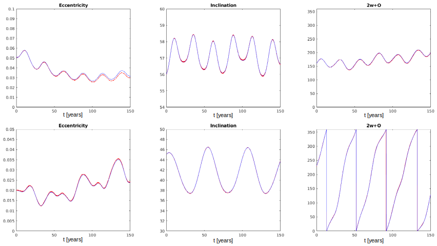
Figure 2. Hamilton’s integration (red lines) vs Cartesian Integration (blue lines). Top: $a=26520$ km, $e=0.05122$, $i=56^{o}$, $\omega=190^{o}$, $\Omega=140^{o}$. Bottom: $a=36700$ km, $e=0.02$, $i=45^{o}$, $\omega=100^{o}$, $\Omega=30^{o}$. Left: eccentricity. Middle: inclination. Right: resonant angle $2\omega+\Omega$.

Figure 2 shows the evolution over 150 years of eccentricity, inclination and resonant angle for two different orbits: the upper one in a 2:1 resonance and the lower one in a non-resonant region. In each case we plot two solutions, one obtained integrating the Cartesian equations and the other one obtained integrating Hamilton’s equations associated to (2.8). The results confirm that the Hamiltonian (2.8) is already accurate enough. This motivates our choice to use a truncated expansion to order $l=2$ within the normalization procedure described in Section 3 and implemented in Section 4.

3. Normalization algorithm

The normalization algorithm is an iterative procedure that transforms a Hamiltonian function, using canonical coordinates changes, so that the transformed Hamiltonian takes a prescribed form, for example that it is integrable up to a remainder term. The normalization algorithm can be iterated with the goal to reduce the size of the remainder term, although we must be aware that the procedure is not converging in general ([41]) and that the computational complexity increases as the number of normalization steps becomes higher.

We adopt a normalization algorithm based on the use of Lie series (see, e.g., [15]); although it is a standard procedure, we briefly recall the normal form algorithm, since it is at the basis of the computation of the proper elements.

Let $\mathcal{H}=\mathcal{H}({\underline{I}},{\underline{\varphi}})$ be a Hamiltonian function defined in terms of action-angle variables $({\underline{I}},{\underline{\varphi}})\in B\times{\mathbb{T}}^{n}$, where $B\subset{\mathbb{R}}^{n}$ is an open set and $n$ denotes the number of degrees of freedom. We write the Hamiltonian as

$$\mathcal{H}({\underline{I}},{\underline{\varphi}})=\mathcal{H}_{0}({\underline{I}})+\varepsilon\mathcal{H}_{1}({\underline{I}},{\underline{\varphi}})\ ,$$ (3.1)

where $\mathcal{H}_{0}({\underline{I}})$ represents the integrable part, $\mathcal{H}_{1}({\underline{I}},{\underline{\varphi}})$ is the perturbing term and $\varepsilon$ represents a small parameter. We assume that $\mathcal{H}_{1}$ is the sum of products between functions depending on actions and cosines of different combinations of angles; hence, $\mathcal{H}_{1}$ can be expanded in Fourier series as

$$\mathcal{H}_{1}({\underline{I}},{\underline{\varphi}})=\sum_{{\underline{k}}\in\mathcal{K}}b_{\underline{k}}({\underline{I}})\exp(\mathit{i}{\underline{k}}\cdot{\underline{\varphi}})\ ,$$ (3.2)

where $\mathcal{K}\subseteq\mathbb{Z}^{n}$ and $b_{\underline{k}}$ denote functions with real coefficients.

We look for a canonical transformation with generating function $\chi$ that allows us to perform the change of variables from $({\underline{I}},{\underline{\varphi}})$ to $({\underline{I}}^{\prime},{\underline{\varphi}}^{\prime})$ defined through the expressions

$${\underline{I}}=S_{\chi}^{\varepsilon}{\underline{I}}^{\prime}\ ,\qquad{\underline{\varphi}}=S_{\chi}^{\varepsilon}{\underline{\varphi}}^{\prime}\ ,$$ (3.3)

where the operator $S_{\chi}^{\varepsilon}\mathcal{F}$ is defined by

$$S_{\chi}^{\varepsilon}\mathcal{F}:=\mathcal{F}+\sum_{i=1}^{\infty}\frac{\varepsilon^{i}}{i!}\{\{\dots\{\mathcal{F},\chi\},\dots\},\chi\}\ ,$$

and $\{\cdot,\cdot\}$ is the Poisson bracket operator, such that $\{\mathcal{F},\chi\}=\sum_{j=1}^{n}{{\partial\mathcal{F}}\over{\partial\varphi_{j}}}{{\partial\chi}\over{\partial I_{j}}}-{{\partial\mathcal{F}}\over{\partial I_{j}}}{{\partial\chi}\over{\partial\varphi_{j}}}$.

The function $S_{\chi}^{\varepsilon}$ must be chosen so that the transformed Hamiltonian $\mathcal{H}^{(1)}=S_{\chi}^{\varepsilon}\mathcal{H}$ takes the following expression:

$$\mathcal{H}^{(1)}({\underline{I}}^{\prime},{\underline{\varphi}}^{\prime})=\mathcal{H}_{0}({\underline{I}}^{\prime})+\varepsilon\overline{\mathcal{H}}_{1}({\underline{I}}^{\prime})+\varepsilon^{2}\mathcal{H}_{2}({\underline{I}}^{\prime},{\underline{\varphi}}^{\prime})\ ,$$ (3.4)

where $\mathcal{H}_{0}+\varepsilon\overline{\mathcal{H}}_{1}$ is the new integrable Hamiltonian (depending just on the new actions) and $\mathcal{H}_{2}$ is the remainder term (the overbar denotes the average with respect to the angles).

Inserting the transformation (3.3) into (3.1), and expanding in Taylor series in the parameter $\varepsilon$, one obtains that the transformed Hamiltonian is given by

$$\mathcal{H}^{(1)}({\underline{I}}^{\prime},{\underline{\varphi}}^{\prime}) = \mathcal{H}_{0}({\underline{I}}^{\prime})+\varepsilon\mathcal{H}_{1}({\underline{I}}^{\prime},{\underline{\varphi}}^{\prime})+\varepsilon\{\mathcal{H}_{0}({\underline{I}}^{\prime}),\chi({\underline{I}}^{\prime},{\underline{\varphi}}^{\prime})\}+\varepsilon^{2}\{\mathcal{H}_{1}({\underline{I}}^{\prime},{\underline{\varphi}}^{\prime}),\chi({\underline{I}}^{\prime},{\underline{\varphi}}^{\prime})\}$$ (3.5)

$$+ \frac{\varepsilon^{2}}{2}\{\{\mathcal{H}_{0}({\underline{I}}^{\prime}),\chi({\underline{I}}^{\prime},{\underline{\varphi}}^{\prime})\},\chi({\underline{I}}^{\prime},{\underline{\varphi}}^{\prime})\}+\dots$$

To obtain a Hamiltonian function of the form (3.4), we must impose that the function in (3.5), that contains only terms of first order in $\varepsilon$, does not depend on the angles. This allows us to determine the generating function $\chi$ as the solution of the following homological equation:

$$\mathcal{H}_{1}({\underline{I}}^{\prime},{\underline{\varphi}}^{\prime})+\{\mathcal{H}_{0}({\underline{I}}^{\prime}),\chi({\underline{I}}^{\prime},{\underline{\varphi}}^{\prime})\}=\overline{\mathcal{H}}_{1}({\underline{I}}^{\prime})\ .$$ (3.6)

Taking into account the expression (3.2) for $\mathcal{H}_{1}$, we look for a generating function of the form

$$\chi({\underline{I}}^{\prime},{\underline{\varphi}}^{\prime})=\sum_{\underline{k}\in\mathbb{Z}^{n}\backslash\{\underline{0}\}}c_{\underline{k}}({\underline{I}}^{\prime})\exp(\mathit{i}\underline{k}\cdot{\underline{\varphi}}^{\prime})\ ,$$ (3.7)

where the coefficients $c_{\underline{k}}$ will be determined through (3.6). In fact, denoting by $\underline{\omega}_{0}={{\partial\mathcal{H}_{0}}\over{\partial{\underline{I}}^{\prime}}}$, we obtain

$$\{\mathcal{H}_{0}({\underline{I}}^{\prime}),\chi({\underline{\varphi}}^{\prime},{\underline{I}}^{\prime})\}=-\mathit{i}\sum_{\underline{k}\in\mathbb{Z}^{n}\backslash\{\underline{0}\}}c_{\underline{k}}({\underline{I}}^{\prime})\ \underline{k}\cdot{\underline{\omega}}_{0}\ \exp(\mathit{i}{\underline{k}}\cdot{\underline{\varphi}}^{\prime})\ .$$ (3.8)

Then, equation (3.6) is satisfied provided the coefficients $c_{\underline{k}}$ are defined as

$$c_{\underline{k}}({\underline{I}}^{\prime})=-\mathit{i}\frac{b_{\underline{k}}({\underline{I}}^{\prime})}{\underline{k}\cdot{\underline{\omega}}_{0}}\ ,\qquad{\underline{k}\not=\underline{0}}\ .$$ (3.9)

Hence, the generating function takes the form

$$\chi({\underline{I}}^{\prime},{\underline{\varphi}}^{\prime})=-\sum_{\underline{k}\in\mathbb{Z}^{n}\backslash\{\underline{0}\}}\mathit{i}\frac{b_{\underline{k}}({\underline{I}}^{\prime})}{\underline{k}\cdot{\underline{\omega}}_{0}}\ \exp(\mathit{i}\underline{k}\cdot{\underline{\varphi}}^{\prime})\ .$$ (3.10)

As a consequence, the new Hamiltonian takes the form (3.4). If one discards the terms of order $\varepsilon^{2}$, the normal form is integrable up to orders of $\varepsilon^{2}$.

If, instead, we keep the terms of order $\varepsilon^{2}$, we can iterate the procedure to higher orders to improve the accuracy of the Hamiltonian normal form. In this case, the new integrable part is given by $\mathcal{H}_{0}({\underline{I}}^{\prime})+\varepsilon\overline{\mathcal{H}}_{1}({\underline{I}}^{\prime})$ and the perturbation is the reminder $\varepsilon^{2}\mathcal{H}_{2}({\underline{I}}^{\prime},{\underline{\varphi}}^{\prime})$. The algorithm will provide a new generating function that can be constructed explicitly, using a procedure similar to that leading to (3.10).

4. Proper elements in a non-resonant region

In this Section, we apply the normalization algorithm described in Section 3 and we compute the proper elements for several samples of space debris in a non-resonant region of the phase space; we remind that the proper elements are the quasi-integrals of the Hamiltonian function describing the dynamics of the space debris. More precisely, we will compute exact integrals of the non-resonant normal form (namely, of the integrable part) which, when expressed in terms of the original elements, are almost conserved quantities up to order $\varepsilon^{N+1}$, where $N$ is the normalization order.

After describing the computation of the proper elements in Section 4.1, we consider three different samples at increasing altitudes (see Sections 4.3, 4.4); these samples are composed by a number of fragments generated after a break-up event, which is obtained through the simulator briefly described in Section 4.2 and developed in [1], using the procedure presented in [24].

The distribution of the proper elements at different times of the evolution of the propagation of the fragments will be presented later in Section 6.4.

4.1. Computation of the proper elements

We consider objects belonging to regions not affected by tesseral resonances, so that the normalization procedure described in Section 3 applies straightforwardly. For the elements of Sun and Moon, we will use the data given in Table 2. The results of this Section concern break-up events and their propagation obtained by considering the model including the geopotential, Sun and Moon. Hence, in this Section the normalization procedure does not include SRP, which will be discussed in Section 6.2, where we will mention the modifications needed in the normalization to include the effect of SRP.

	Sun	Moon
Mean daily motion	$1^{o}/day$	$13.06^{o}/day$
Semi-major axis	$1.496\cdot 10^{8}$ km	$384478$ km
Eccentricity	0.0167	0.0549
Inclination	$23^{o}26^{\prime}21.406^{\prime\prime}$	$5^{o}15^{\prime}$
$\dot{\omega}_{S/M}$	$282.94^{o}/day$	$0.164^{o}/day$
$\dot{\Omega}_{S/M}$	$0^{o}/day$	$-0.0529918^{o}/day$

Table 2. Orbital elements of Sun and Moon.

The first step consists in averaging the expansions (2.1), (2.5), (2.6) (truncated to order $l=2$) over the fast and semi-fast angles, namely the mean anomalies $M$, $M_{S}$, $M_{M}$, and the sidereal time $\theta$. As a consequence of the averaging over $M$, the semi-major axis is constant for the approximate averaged Hamiltonian and becomes the first proper element.

Due to the fact that the quantity $\Omega_{M}$ depends on time with constant rate $\dot{\Omega}_{M}=-0.0529918^{o}/day$ (as shown in Table 2), after averaging we end-up with the following Hamiltonian function:

$${\overline{\mathcal{H}}}(e,i,\omega,\Omega,t)=\mathcal{H}_{E}^{sec}(e,i,\omega,\Omega)+{\overline{\mathcal{H}}}_{S}(e,i,\omega,\Omega)+{\overline{\mathcal{H}}}_{M}(e,i,\omega,\Omega,t)\ ,$$

where $\mathcal{H}_{E}^{sec}$ is given by (2.4) and includes terms depending on $J_{2}$ and $J_{3}$.

Let us introduce the Delaunay action variables defined as

$$L=\sqrt{\mu_{E}a}\ ,\qquad G=L\sqrt{1-e^{2}}\ ,\qquad H=G\cos i\ ;$$

the conjugated angle variables are $M$, $\omega$, $\Omega$. In terms of such variables, we get a two degrees of freedom, time-dependent Hamiltonian of the form:

$${\overline{\mathcal{H}}}(G,H,\omega,\Omega,t)=\mathcal{H}_{E}^{sec}(G,H,\omega,\Omega)+{\overline{\mathcal{H}}}_{S}(G,H,\omega,\Omega)+{\overline{\mathcal{H}}}_{M}(G,H,\omega,\Omega,t)\ .$$

In the light of the theory presented in Section 3, it is convenient to transform the Hamiltonian so that it becomes autonomous. To do this, we premise that our unit of time is one sidereal day over $2\pi$ and that the angles are measured in radians; since in Table 2 the rate of variation of the longitude of the ascending node is given in degrees/synodic day, we transform such value as $-0.0529918\cdot 365.242196/(366.242196\cdot 360)$, which gives the value of $-0.000146798$ rad/(sidereal day). This motivates the introduction of an angle variable defined as $\Omega_{M}=-0.000146798\,t$, which represents the linear evolution of the node of the Moon in our time units; we denote by $H_{M}$ its conjugated action variable. Then, the extended Hamiltonian is given by

$${\overline{\mathcal{H}}}_{ext}(G,H,H_{M},\omega,\Omega,\Omega_{M}) = \mathcal{H}_{E}^{sec}(G,H,\omega,\Omega)+{\overline{\mathcal{H}}}_{S}(G,H,\omega,\Omega)$$

$$+ {\overline{\mathcal{H}}}_{M}(G,H,\omega,\Omega,\Omega_{M})-0.000146798\,H_{M}\ .$$

Next, we make a linear (canonical) change of coordinates to consider the dynamics around fixed reference values of $G$ and $H$, say $G_{0}$ and $H_{0}$. Thus, the transformation of coordinates $(G,H)\to(P+G_{0},Q+H_{0})$ leads to introduce new variables $(P,Q)$, which are close to zero. To keep a consistent notation, we use $(Q_{M},p,q,q_{M})$ instead of $(H_{M},\omega,\Omega,\Omega_{M})$. In this notation, in the neighborhood of $G_{0}$, $H_{0}$, the Hamiltonian function can be written as

$${\overline{\mathcal{H}}}_{ext}(P+G_{0},Q+H_{0},Q_{M},p,q,q_{M}) = \mathcal{H}_{E}^{sec}(P+G_{0},Q+H_{0},p,q)+{\overline{\mathcal{H}}}_{S}(P+G_{0},Q+H_{0},p,q)$$

$$+ {\overline{\mathcal{H}}}_{M}(P+G_{0},Q+H_{0},p,q,q_{M})-0.000146798\,Q_{M}\ ,$$

that we expand in power series around $P=0$ and $Q=0$ up to order 3 in $P$ and $Q$, separately. We call ${\overline{\mathcal{H}}}$ the expanded Hamiltonian.

The linear part in the action variables of the Hamiltonian, that we denote by $Z_{0}$, can be expressed in the form:

$$Z_{0}(P,Q,Q_{M})=\nu_{P}\,P+\nu_{Q}\,Q+\nu_{Q_{M}}\,Q_{M}\ ,$$

where the ‘frequencies’ $\nu_{P}$, $\nu_{Q}$, $\nu_{Q_{M}}$ are functions of $L_{0}$, $G_{0}$, $H_{0}$. The explicit expressions for the frequencies are the following:

$$\nu_{P}(L_{0},G_{0},H_{0}) = \frac{0.92\cdot 10^{-4}H_{0}^{2}}{G_{0}^{6}L_{0}^{3}}-\frac{0.18\cdot 10^{-4}}{G_{0}^{4}L_{0}^{3}}+\frac{0.33\cdot 10^{-4}H_{0}^{2}L_{0}^{4}}{G_{0}^{3}}-0.67\cdot 10^{-4}G_{0}L_{0}^{2}\ ,$$

$$\nu_{Q}(L_{0},G_{0},H_{0}) = -\frac{0.37\cdot 10^{-4}H_{0}}{G_{0}^{5}L_{0}^{3}}-\frac{0.33\cdot 10^{-4}H_{0}L_{0}^{4}}{G_{0}^{2}}+0.20\cdot 10^{-4}H_{0}L_{0}^{2}\ ,$$

$$\nu_{Q_{M}} = -1.46798\cdot 10^{-4}\ .$$

We remind that the units of length and time are normalized by setting the geostationary distance of $42164.1696$ km equal to one and the period of Earth’s rotation equal to $2\pi$; this choice implies $\mu_{E}=1$.

Next, we split the Hamiltonian into two parts, namely $Z_{0}$ and a remainder $R_{0}$. In this way we end up with a Hamiltonian of the form (3.1), namely

$$\mathcal{H}(P,Q,Q_{M},p,q,q_{M})=Z_{0}(P,Q,Q_{M})+R_{0}(P,Q,Q_{M},p,q,q_{M})\ .$$ (4.1)

Given that the Hamiltonian in (4.1) is obtained as the sum of two contributions with the norm of $R_{0}$ typically (much) smaller than the norm of $Z_{0}$, following [15], we introduce a book-keeping parameter $\lambda$ in front of $R_{0}$. More precisely, the book-keeping parameter is introduced to label the part of the Hamiltonian which has to be removed by the normalization algorithm. Therefore, following the procedure described in Section 3, at each normalization step we split the remainder into two parts, the first one depending just on the actions and the second one depending on all variables. Performing the steps (3.6)-(3.9), we compute the generating function and the transformed Hamiltonian.

If we stop the iteration of the normalization procedure, we retain the Hamiltonian parts containing only the terms independent on $\lambda$ and the terms linear in $\lambda$. Since the introduction of the book-keeping was fictitious, at the end we restore its value to $\lambda=1$.

If, instead, we decide to perform another normalization step, the terms of second order in $\lambda$ are used to label the remainder and the normalization method is then iterated. Once we finish the iteration, we use the generating functions computed at each normalization step to find the other two proper elements, namely the proper eccentricity and the proper inclination.

To be more specific, let us denote by $N$ the number of steps of the normalization procedure (in practical computations we will take $N=1$). Denoting with a prime the variables after the normalizing transformation, we end-up with a Hamiltonian of the form

$${\mathcal{H}}^{(N)}(P^{\prime},Q^{\prime},Q_{M}^{\prime},p^{\prime},q^{\prime},q_{M}^{\prime})=Z^{(N)}(P^{\prime},Q^{\prime},Q_{M}^{\prime})+R^{(N)}(P^{\prime},Q^{\prime},Q_{M}^{\prime},p^{\prime},q^{\prime},q_{M}^{\prime})\ ,$$ (4.2)

where $Z^{(N)}=Z_{0}(P^{\prime},Q^{\prime},Q_{M}^{\prime})+\lambda Z_{1}(P^{\prime},Q^{\prime},Q_{M}^{\prime})+\dots+\lambda^{N}Z_{N}(P^{\prime},Q^{\prime},Q_{M}^{\prime})$ is the normal form at order $N$, depending just on the actions, and $R^{(N)}=\lambda^{N+1}R_{N}(P^{\prime},Q^{\prime},Q_{M}^{\prime},p^{\prime},q^{\prime},q_{M}^{\prime})$ is the remainder; again, $\lambda$ denotes the book-keeping parameter, that will be set equal to one at the end of the procedure. If we disregard $R^{(N)}$, we obtain that $P^{\prime}$, $Q^{\prime}$, $Q_{M}^{\prime}$ are constants of motion for the Hamiltonian ${\mathcal{H}}_{0}^{(N)}=Z^{(N)}(P^{\prime},Q^{\prime},Q_{M}^{\prime})$, while $p^{\prime}$, $q^{\prime}$, $q_{M}^{\prime}$ evolve linearly in time. Hence, we can write the solution of Hamilton’s equations associated to ${\mathcal{H}}_{0}^{(N)}$ as

$$P^{\prime}(t) =P_{0}^{\prime}$$

$$Q^{\prime}(t) =Q_{0}^{\prime}$$

$$Q_{M}^{\prime}(t) =Q_{M,0}^{\prime}$$

$$p^{\prime}(t) =p_{0}^{\prime}+\dfrac{\partial Z^{(N)}}{\partial P^{\prime}}(P^{\prime}_{0},Q^{\prime}_{0},Q_{M,0}^{\prime})\ t$$

$$q^{\prime}(t) =q_{0}^{\prime}+\dfrac{\partial Z^{(N)}}{\partial Q^{\prime}}(P^{\prime}_{0},Q^{\prime}_{0},Q_{M,0}^{\prime})\ t$$

$$q_{M}^{\prime}(t) =q_{M,0}^{\prime}+\dfrac{\partial Z^{(N)}}{\partial Q_{M}^{\prime}}(P^{\prime}_{0},Q^{\prime}_{0},Q_{M,0}^{\prime})\ t\ ,$$

where $P^{\prime}_{0},Q^{\prime}_{0},Q_{M,0}^{\prime},p_{0}^{\prime},q_{0}^{\prime},q_{M,0}^{\prime}$ denote the initial conditions. To compute the original variables as a function of the new variables, we use the generating functions that led to (4.2) and that we denote as $\chi^{(N)},\chi^{(N-1)},\dots,\chi^{(1)}$ ([17]). Hence, we obtain

$$P(P^{\prime}(t),Q^{\prime}(t),Q_{M}^{\prime}(t),p^{\prime}(t),q^{\prime}(t),q_{M}^{\prime}(t))=S^{\lambda}_{\chi^{(1)}}\circ\dots\circ S^{\lambda}_{\chi^{(N)}}P^{\prime},$$

$$Q(P^{\prime}(t),Q^{\prime}(t),Q_{M}^{\prime}(t),p^{\prime}(t),q^{\prime}(t),q_{M}^{\prime}(t))=S^{\lambda}_{\chi^{(1)}}\circ\dots\circ S^{\lambda}_{\chi^{(N)}}Q^{\prime},$$

$$Q_{M}(P^{\prime}(t),Q^{\prime}(t),Q_{M}^{\prime}(t),p^{\prime}(t),q^{\prime}(t),q_{M}^{\prime}(t))=S^{\lambda}_{\chi^{(1)}}\circ\dots\circ S^{\lambda}_{\chi^{(N)}}Q_{M}^{\prime},$$

$$p(P^{\prime}(t),Q^{\prime}(t),Q_{M}^{\prime}(t),p^{\prime}(t),q^{\prime}(t),q_{M}^{\prime}(t))=S^{\lambda}_{\chi^{(1)}}\circ\dots\circ S^{\lambda}_{\chi^{(N)}}p^{\prime},$$

$$q(P^{\prime}(t),Q^{\prime}(t),Q_{M}^{\prime}(t),p^{\prime}(t),q^{\prime}(t),q_{M}^{\prime}(t))=S^{\lambda}_{\chi^{(1)}}\circ\dots\circ S^{\lambda}_{\chi^{(N)}}q^{\prime},$$

$$q_{M}(P^{\prime}(t),Q^{\prime}(t),Q_{M}^{\prime}(t),p^{\prime}(t),q^{\prime}(t),q_{M}^{\prime}(t))=S^{\lambda}_{\chi^{(1)}}\circ\dots\circ S^{\lambda}_{\chi^{(N)}}q_{M}^{\prime}\ ,$$

which implies that we can express the original variables as

$$P(P^{\prime}(t),Q^{\prime}(t),Q_{M}^{\prime}(t),p^{\prime}(t),q^{\prime}(t),q_{M}^{\prime}(t))=\tilde{P}(P_{0}^{\prime},Q_{0}^{\prime},Q_{M,0}^{\prime},p_{0}^{\prime},q_{0}^{\prime},q_{M,0}^{\prime},t),$$ (4.3)

$$Q(P^{\prime}(t),Q^{\prime}(t),Q_{M}^{\prime}(t),p^{\prime}(t),q^{\prime}(t),q_{M}^{\prime}(t))=\tilde{Q}(P_{0}^{\prime},Q_{0}^{\prime},Q_{M,0}^{\prime},p_{0}^{\prime},q_{0}^{\prime},q_{M,0}^{\prime},t),$$

$$Q_{M}(P^{\prime}(t),Q^{\prime}(t),Q_{M}^{\prime}(t),p^{\prime}(t),q^{\prime}(t),q_{M}^{\prime}(t))=\tilde{Q}_{M}(P_{0}^{\prime},Q_{0}^{\prime},Q_{M,0}^{\prime},p_{0}^{\prime},q_{0}^{\prime},q_{M,0}^{\prime},t),$$

$$p(P^{\prime}(t),Q^{\prime}(t),Q_{M}^{\prime}(t),p^{\prime}(t),q^{\prime}(t),q_{M}^{\prime}(t))=\tilde{p}(P_{0}^{\prime},Q_{0}^{\prime},Q_{M,0}^{\prime},p_{0}^{\prime},q_{0}^{\prime},q_{M,0}^{\prime},t),$$

$$q(P^{\prime}(t),Q^{\prime}(t),Q_{M}^{\prime}(t),p^{\prime}(t),q^{\prime}(t),q_{M}^{\prime}(t))=\tilde{q}(P_{0}^{\prime},Q_{0}^{\prime},Q_{M,0}^{\prime},p_{0}^{\prime},q_{0}^{\prime},q_{M,0}^{\prime},t),$$

$$q_{M}(P^{\prime}(t),Q^{\prime}(t),Q_{M}^{\prime}(t),p^{\prime}(t),q^{\prime}(t),q_{M}^{\prime}(t))=\tilde{q}_{M}(P_{0}^{\prime},Q_{0}^{\prime},Q_{M,0}^{\prime},p_{0}^{\prime},q_{0}^{\prime},q_{M,0}^{\prime},t)\ ,$$

where, by using the solutions of the normal form equations, the functions $\tilde{P}$, $\tilde{Q}$, $\tilde{Q}_{M}$, $\tilde{p}$, $\tilde{q}$, $\tilde{q}_{M}$ are explicit functions of time. To compute $P_{0}^{\prime},Q_{0}^{\prime},Q_{M,0}^{\prime},p_{0}^{\prime},q_{0}^{\prime},q_{M,0}^{\prime}$, we have two possibilities. One is to compute the inverse transformation by exploiting the generating functions; however, for a low order normalization, this procedure is usually not very accurate. On the other hand, an appropriate method to compute the initial conditions is to solve the following system of equations:

$$\tilde{P}(P_{0}^{\prime},Q_{0}^{\prime},Q_{M,0}^{\prime},p_{0}^{\prime},q_{0}^{\prime},q_{M,0}^{\prime},0)=P_{0},$$

$$\tilde{Q}(P_{0}^{\prime},Q_{0}^{\prime},Q_{M,0}^{\prime},p_{0}^{\prime},q_{0}^{\prime},q_{M,0}^{\prime},0)=Q_{0},$$

$$\tilde{Q}_{M}(P_{0}^{\prime},Q_{0}^{\prime},Q_{M,0}^{\prime},p_{0}^{\prime},q_{0}^{\prime},q_{M,0}^{\prime},0)=Q_{M,0},$$

$$\tilde{p}(P_{0}^{\prime},Q_{0}^{\prime},Q_{M,0}^{\prime},p_{0}^{\prime},q_{0}^{\prime},q_{M,0}^{\prime},0)=p_{0},$$

$$\tilde{q}(P_{0}^{\prime},Q_{0}^{\prime},Q_{M,0}^{\prime},p_{0}^{\prime},q_{0}^{\prime},q_{M,0}^{\prime},0)=q_{0},$$

$$\tilde{q}_{M}(P_{0}^{\prime},Q_{0}^{\prime},Q_{M,0}^{\prime},p_{0}^{\prime},q_{0}^{\prime},q_{M,0}^{\prime},0)=q_{M,0}\ ,$$

which we insert in (4.3) to obtain the analytic solution in the original variables. Finally, from $P(t)$, $Q(t)$, we go back to $G(t)$, $H(t)$ and hence to $e(t)$, $i(t)$. As a last step, we define the proper eccentricity $e_{p}$ and the proper inclination $i_{p}$ as the averages over a given time interval, say $[t_{0},T]$:

$$e_{p}(T)=\frac{1}{T-t_{0}}\int_{t_{0}}^{T}e(t)dt,\qquad i_{p}(T)=\frac{1}{T-t_{0}}\int_{t_{0}}^{T}i(t)dt\ .$$

We remark that we could have also computed the proper elements in the transformed variables, without the need of using the analytic solution to compute the proper elements in terms of the original variables. Having in mind concrete applications, we believe that our procedure is more appropriate, beside being suitable for different purposes, like the propagation of the solution. However, it must be admitted that the direct determination of the proper elements in the transformed variables is computationally simpler and it provides results quite similar to our original procedure.

4.2. A simulator for generating fragments

In the following Sections, we will compute the proper elements associated to several fragments generated by a break-up event. To this end, our results are obtained using a simulator of collisions developed within the ongoing collaboration in [1], which reproduces the break-up model Evolve 4.0 provided by NASA (see [24], [27], [2]). This simulator, which has been validated for debris sizes greater than 1 mm, allows us to determine the cross-sections, masses, and imparted velocities of the fragments after an explosion or a collision.

The break-up model Evolve 4.0 includes:

- the size distribution of the fragments after collision or explosion,

- the fragments’ area-to-mass ratio,

- the fragments’ relative velocity distribution with respect to the parent body.

Due to the fact that the above parameters are not the same for all debris, it is necessary to provide the distributions as a function of a given parameter, e.g. the mass or the characteristic length. Besides, the simulations can be highly influenced by the initial conditions and parameters of the break-up, for example the total mass of the parent body or the collision velocity.

We remark that the explosion and collision rates, as well as the fragment size distribution, affect the production rate of the debris particles. On the other hand, the area-to-mass ratio and the relative velocity distribution affect how the debris evolve and eventually decay.

We refer to [24], [27], [2] for further details on the break-up simulator that we reproduced in [1] to obtain the fragments generated by a collision or an explosion.

In the collision case, the simulator has as inputs the position of the parent body, the mass of both parent and projectile bodies and the impact velocity. In the explosion case, the inputs are just the position and type of the parent satellite (body).

Only fragments bigger than 12 cm are generated. The output that will be produced to obtain the results of Sections 4.3-4.5 is a combination of the simulator of break-up events, the propagation of the fragments’ orbits, and the computation of the proper elements. Precisely, we compute the following three sets of data:

$(i)$ a set of instantaneous velocities after break-up, transformed to the orbital elements of each fragment at the instant of time after the event. In this way, we obtain the distribution of the elements in the phase space of semi-major axis, eccentricity and inclination;

$(ii)$ starting from the data after the break-up, we propagate each fragment for a given period of time, typically up to 150 years. This result allows us to monitor how the distribution evolves;

$(iii)$ we use the position of the fragments after the propagation up to a given interval of time (e.g., 150 years) to compute the proper elements of each fragment. The distribution of the proper elements is then compared to that of the elements at the initial time after the break-up.

Among an extensive survey of cases we have analyzed, we select the three representative samples at different altitudes described in Sections 4.3, 4.4.

4.3. Moderate altitude orbits

In this Section we present two samples obtained by simulating an explosion of a spacecraft of Titan Transtage type and a collision between a 1200 kg parent body and 5 kg projectile at the relative velocity of 4900 m/s.

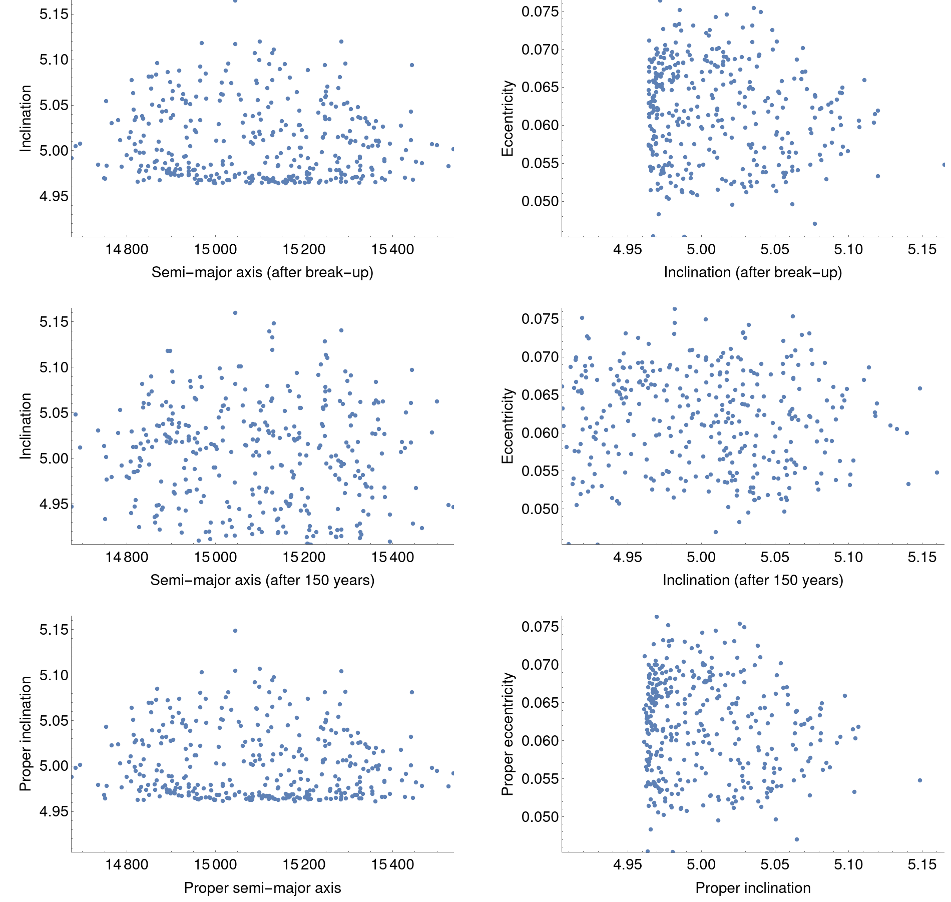
Figure 3. Distribution of $a$-$i$ (left), $i$-$e$ (right) with the parent body at the initial position $a=15100$ km, $e=0.06$, $i=5^{o}$, $\omega=90^{o}$, $\Omega=10^{o}$ after break-up (first row), after 150 years (second row), and proper elements computed after 150 years (third row).

The first sample is located at relatively low distance from the Earth; precisely, we consider a simulated explosion that generates 356 fragments and having the following parameters of the parent body: $a=15100$ km, $e=0.06$, $i=5^{o}$, $\omega=90^{o}$, $\Omega=10^{o}$. The different panels of Figure 3 show the osculating elements immediately after the break-up (first row), the mean elements (obtained by integrating the averaged Hamiltonian) propagated up to 150 years (second row) and the proper elements computed from the evolution after 150 years (third row). The reason for computing the proper elements after a time interval (say, 150 years) relies on the fact that space debris catalogues, like the TLE (Two-Line-Elements) catalogue, provide the values of the elements at a given epoch after the disruptive event and usually not at the time at which the break-up takes place.

Figure 3 illustrates the results in the planes $a$-$i$, $i$-$e$, which show that the proper elements give important information on the distribution of the fragments after the collision. Indeed, after 150 years the debris are spread in phase space (second row), while in the proper element phase space the fragments are restored in groups (third row), similar to those obtained just after break-up (first row). We notice a small shift of the proper inclination, as it happens in most of the examples described in the rest of the work; sometimes the shift occurs also in the eccentricity.

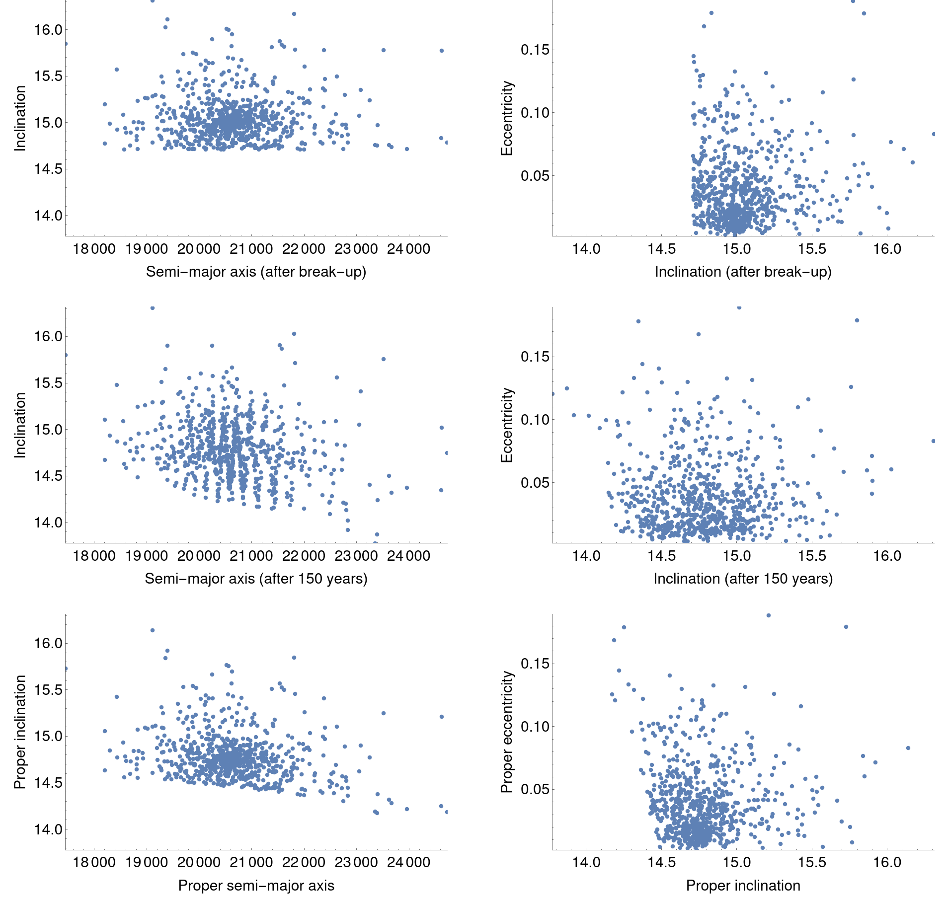
Figure 4. Distribution of $a$-$i$ (left), $i$-$e$ (right) with the parent body at the initial position $a=20600$ km, $e=0.01$, $i=15^{o}$, $\omega=10^{o}$, $\Omega=20^{o}$ after break-up (first row), after 150 years (second row), and proper elements computed after 150 years (third row).

The second sample concerns a collision that generates 767 fragments. The event occurs at a moderate altitude of the parent body with $a=20600$ km and with a relatively small inclination and eccentricity, $e=0.01$, $i=15^{o}$; the other elements are fixed as $\omega=10^{o}$ and $\Omega=20^{o}$.

Figure 4 gives the results in the planes $a$-$i$ and $i$-$e$, where the scales have been fixed as the minimum and the maximum values of the evolution of the elements after 150 years.

A comparison between the panels of the first and second row of Figure 4 shows that the fragments are moderately sparse after a propagation up to 150 years; on the other hand, the proper elements plots look similar to the distribution after the break-up, thus allowing to establish a connection with the fragments at the break-up event.

If we get a closer look at two random fragments as shown in Figure 5, we find that the proper values for the orbital elements are very close to the average values of the evolution of the osculating elements. The evolution of the inclination shows that at a given time the two fragments can be apart by about $1^{o}$, while the proper elements (given by the average inclinations of both fragments) are closer, but nearly constant.

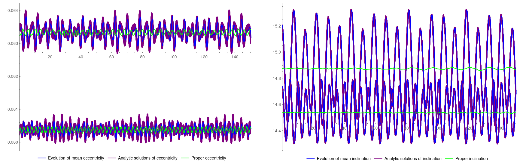
Figure 5. Proper values and evolution of eccentricity and inclination over 150 years of two random fragments ($a=20600$ km, $e=0.01$, $i=15^{o}$, $\omega=10^{o}$, $\Omega=20^{o}$). The blue line is the evolution of the mean elements; the purple line is the analytic solution computed every 6 months; the green line denotes the proper element computed every 6 months.

4.4. Medium altitude orbits

Next case concerns a sample located in the GEO region, between the resonances 2:1 and 1:1. The event has been simulated taking a parent body at $a=33600$ km, $e=0.05$, $i=20^{o}$, $\omega=120^{o}$, $\Omega=60^{o}$ and it consists of an explosion of a spacecraft of Titan Transtage type. After break-up, a total of 356 fragments have been generated.

The results providing the elements at break-up, the propagation after 150 years and the proper elements computed using the data after 150 years are given in Figure 6. The evolution of the osculating elements after 150 years in the $a$-$i$ plane seems to be located around a fitting parabolic curve; instead, the fragments are definitely sparse in the $i$-$e$ plane after 150 years, due to a growth of the inclination from about $15^{o}$ to $22^{o}$. On the contrary, the proper elements in the $a$-$i$ plane take a shape similar to the distribution at the break-up around the value $i=20^{o}$.

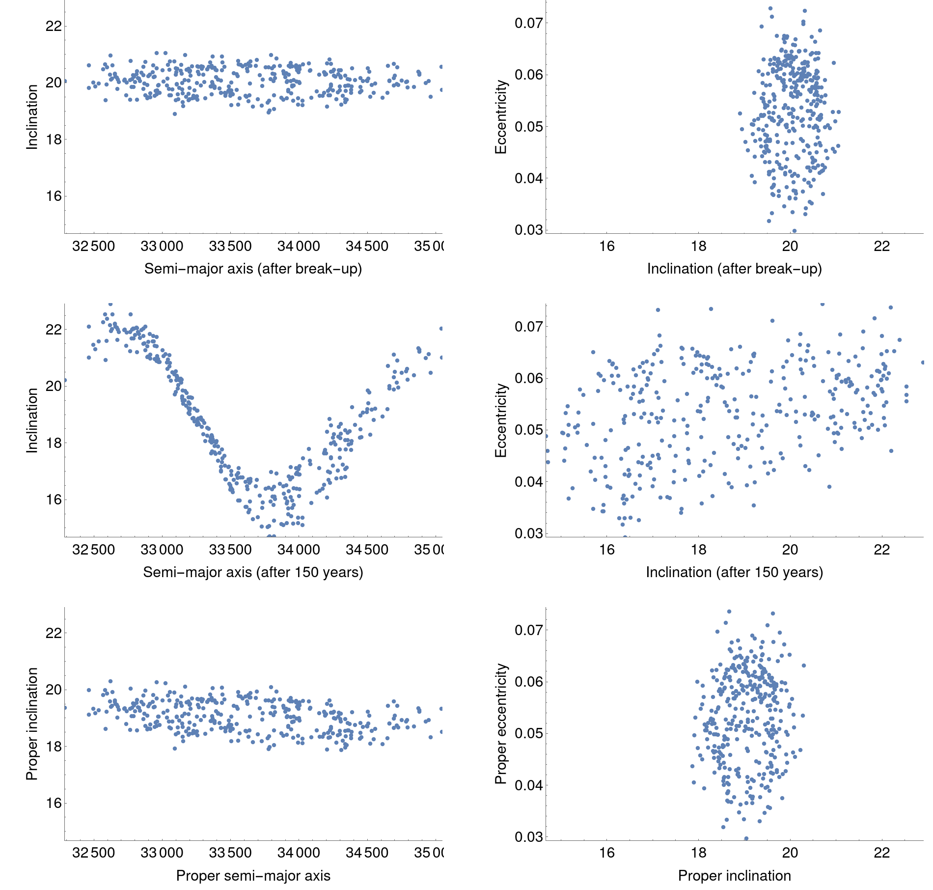
Figure 6. Distribution of $a$-$i$ (left), $i$-$e$ (right) with the parent body at the initial position $a=33600$ km, $e=0.05$, $i=20^{o}$, $\omega=120^{o}$, $\Omega=60^{o}$ after break-up (first row), after 150 years (second row), and proper elements computed after 150 years (third row).

4.5. Identification through fragments’ grouping

An important practical use of the proper elements computation might come from the classification of events taking place at nearby locations. To this end, we simulate in Figure 7 two separate explosions having all elements in common, except the inclination: one explosion occurs at $i=20^{o}$ and the other at $i=21^{o}$. While the evolution after 150 years does not permit to distinguish between the two groups belonging to the original parent bodies, the computation of the proper elements allows us to distinguish two clear groups that closely resemble the distribution of fragments after the break-up.

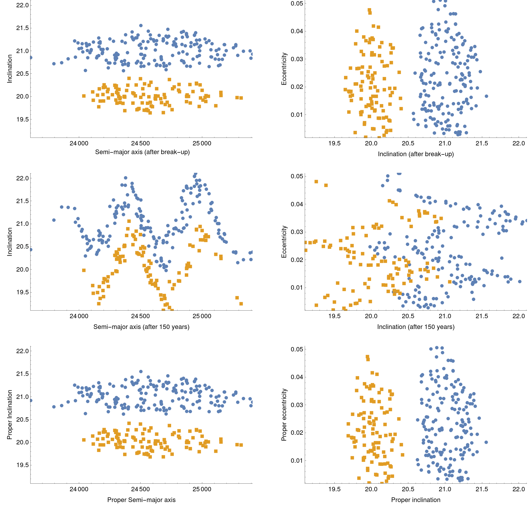
Figure 7. Distribution of $a$-$i$ (left), $i$-$e$ (right) with the parent body at the initial position $a=24600$ km, $e=0.02$, $i=20^{o}$ and $i=21^{o}$, $\omega=110^{o}$, $\Omega=120^{o}$ at break-up (first row), after 150 years (second row) and proper elements computed from data after 150 years (third row).

We also provide a simulation of three explosions occurring at three different inclinations, precisely $i=20^{o}$, $i=21^{o}$, $i=22^{o}$. Also in this case, see Figure 8, the proper elements computation allows us to get information on the existence of three different groups, which correspond to the three different explosions.

These two simple examples confirm the validity of the computation of the proper elements for space debris, as already witnessed by the results on the identification of asteroid families; the formation of groups, as well as their resemblance with the dynamical plots after the break-up, might be used to reconstruct the catastrophic event and to identify the origin of the fragments.

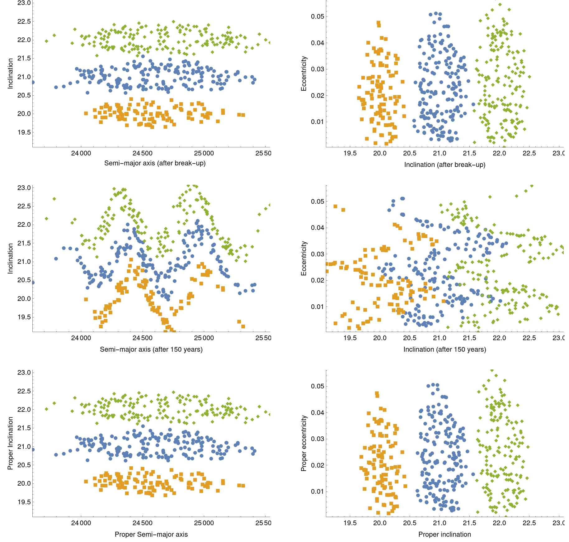
Figure 8. Distribution of $a$-$i$ (left), $i$-$e$ (right) with the parent body at the initial position $a=24600$ km, $e=0.02$, $i=20^{o}$, $i=21^{o}$, $i=22^{o}$, $\omega=110^{o}$, $\Omega=120^{o}$ at break-up (first row), after 150 years (second row) and proper elements computed from data after 150 years (third row).

5. Proper elements close to a tesseral resonance

In this Section, we focus on break-up events taking place close to tesseral resonances. The procedure to construct the normal form will be the same as in Section 4, since our aim is to see if the computation of the proper eccentricity and the proper inclination can be still used to reconstruct the initial distribution after the break-up event.

Tesseral resonances have a strong influence on the evolution of semi-major axis, while their effect is less important for inclination and eccentricity. We include the effect of the tesseral resonance in the computation of the evolution as described in the following Sections.

5.1. Close to the 2:1 tesseral resonance

We start by analyzing the behavior close to the 2:1 tesseral resonance. We remind that the 2:1 tesseral resonance occurs whenever there is a commensurability relation between the mean motion of the space debris, the sidereal time, the argument of perigee and the longitude of the ascending node:

$$\dot{M}-2\dot{\theta}+2\dot{\Omega}+\dot{\omega}=0\ .$$

We remark that when $J_{2}=0$, then $\dot{\omega}=\dot{\Omega}=0$ and the resonance relation reduces to

$$\dot{M}-2\dot{\theta}=0\ .$$

A multiplet tesseral resonance (see [13]) occurs whenever the following relation is satisfied for $\ell\in{\mathbb{Z}}\backslash\{0\}$:

$$\dot{M}-2\dot{\theta}+2\dot{\Omega}+\dot{\omega}+\ell\dot{\omega}=0\ .$$

For the 2:1 resonance, we consider a Hamiltonian function composed by the following terms: the Keplerian part, the resonant Hamiltonian limited to the most important terms, the secular Hamiltonian, the contributions of Sun and Moon that we limit to the Hamiltonians averaged over the corresponding satellite mean anomaly. With respect to the latter choice, we remark that we could have inserted the complete Sun and Moon Hamiltonians, but we noticed that the non-average terms do not contribute much to the dynamics, while they remarkably increase the complexity of the normalization procedure. In summary, in the proximity of the 2:1 resonance, we consider the following Hamiltonian:

$$\mathcal{H}(L,G,H,M,\omega,\Omega,\theta,t) = \mathcal{H}_{Kep}(L)+\mathcal{H}_{E}^{res2:1}(L,G,H,M,\omega,\Omega,\theta)+\mathcal{H}_{E}^{sec}(G,H,\omega,\Omega)$$

$$+ {\overline{\mathcal{H}}}_{S}(G,H,\omega,\Omega)+{\overline{\mathcal{H}}}_{M}(G,H,\omega,\Omega,t)\ ,$$

where the expansion (in the Keplerian orbital elements) of the term $\mathcal{H}_{E}^{res2:1}$ up to order $n=m=3$ and second order in eccentricity (including multiplet resonant terms) is given by

$$\mathcal{H}_{E}^{res2:1} = \frac{J_{22}\mu_{E}R_{E}^{2}}{a^{3}}\left(\frac{9}{8}e\left(2-2\cos^{2}(i)\right)\cos\left(-2\lambda_{22}+2\Omega-2\theta+M\right)\right.$$

$$- \left.\frac{3}{8}e\left(\cos^{2}(i)+2\cos(i)+1\right)\cos\left(-2\lambda_{22}+2\Omega-2\theta+M+2\omega\right)\right)$$

$$+ \frac{J_{32}\mu_{E}R_{E}^{3}}{a^{4}}\left(\frac{165}{64}e^{2}\sin(i)\left(3\cos^{2}(i)-2\cos(i)-1\right)\sin\left(-2\lambda_{32}+2\Omega-2\theta+M-\omega\right)\right.$$

$$+ \left.\frac{15}{64}e^{2}\sin(i)\left(\cos^{2}(i)+2\cos(i)+1\right)\sin\left(-2\lambda_{32}+2\Omega-2\theta+M+3\omega\right)\right.$$

$$+ \left.\frac{15}{8}\left(2e^{2}+1\right)\sin(i)\left(-3\cos^{2}(i)-2\cos(i)+1\right)\sin\left(-2\lambda_{32}+2\Omega-2\theta+M+\omega\right)\right)\ .$$

When the inclination is not too small, the largest term in (5.1) is the last one containing the resonant angle, which appears with the $J_{32}$ coefficient. On the other hand, as shown in [8], there are other two terms, depending respectively on the combinations of the angles $M-2\theta+2\Omega$ and $M-2\theta+2\Omega+2\omega$, which might be important for specific values of eccentricity and inclination. This leads to retain, in the first approximation, only three terms in the initial Hamiltonian $\mathcal{H}_{E}^{res2:1}$. Hence, the Hamiltonian used for the computation of the evolution of the elements is the following:

$$\mathcal{H}(L,G,H,H_{M},M,g,h,h_{M},\theta)=-\frac{\mu_{E}^{2}}{2L^{2}}+\frac{J_{2}\mu_{E}^{4}R_{E}^{2}\left(G^{2}-3H^{2}\right)}{4G^{5}L^{3}}+\mathcal{H}_{S}(G,H,g,h)$$

$$+\mathcal{H}_{M}(G,H,g,h,h_{M})-0.000146798H_{M}+\frac{3}{64G^{2}L^{10}}\left(5J_{32}\mu_{E}^{5}R_{E}^{3}\right.$$

$$\left.\sqrt{1-\frac{H^{2}}{G^{2}}}\left(-8\left(G^{2}-2GH-3H^{2}\right)\left(2G^{2}-3L^{2}\right)\sin\left(-2\lambda_{32}+2\Omega-2\theta+M+\omega\right)\right)\right.$$

$$\left.+8L^{4}J_{22}\mu_{E}^{4}R_{E}^{2}\sqrt{1-\frac{G^{2}}{L^{2}}}\left(6(G^{2}-H^{2})\cos(-2\lambda_{22}+2\Omega-2\theta+M)\right.\right.$$

$$\left.\left.-(G+H)^{2}\cos\left(-2\lambda_{22}+2\Omega-2\theta+M+2\omega\right)\right)\right)\ .$$

Figure 9 shows an experiment analyzing an explosion of a spacecraft of Titan Transtage type orbiting at $a=26600$ km, $e=0.07$, $i=15^{o}$, $\omega=270^{o}$, $\Omega=120^{o}$. The dynamics around the 2:1 tesseral resonance is chaotic, as shown by the sinusoidal distribution in the $a$-$i$ plane and from the spreading of fragments in inclination in Figure 9. On the other hand, looking at the third row of Figure 9, we notice a quite successful computation of proper elements for almost all fragments. However, we are aware of the fact that we did not obtain an accurate reconstruction of the initial distribution, due to the fact that some fragments could be very close to the resonant region, either inside it. We believe that the computation of the proper elements close to a resonance might be improved by using an appropriate resonant normal form procedure.

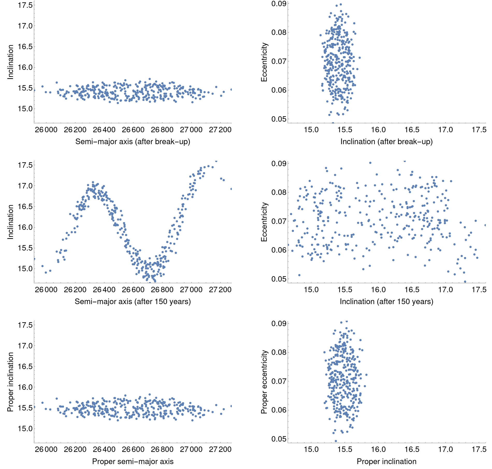
Figure 9. Distribution of $a$-$i$ (left), $i$-$e$ (right) with the parent body at the initial position $a=26600$ km, $e=0.07$, $i=15^{o}$, $\omega=270^{o}$, $\Omega=120^{o}$ after break-up (first row), after 150 years (second row), and proper elements computed after 150 years (third row).

5.2. Close to the 1:1 tesseral resonance

In this Section, we shortly analyze the dynamics close to the 1:1 tesseral resonance, which contains many resonant terms, but only a single dominant one, as described in [8]. The dominant term is given by the expression:

$$\mathcal{H}_{E}^{res1:1}={{J_{22}\mu_{E}R_{E}^{2}}\over a^{3}}\left.\frac{3}{4}\left(1-\frac{5e^{2}}{2}\right)\left(\cos^{2}(i)+2\cos(i)+1\right)\cos\left(-2\lambda_{22}+2\Omega-2\theta+2M+2\omega\right)\right)\ ,$$

which leads to consider the following Hamiltonian:

$$\mathcal{H}(L,G,H,l,g,h,\theta,h_{M},H_{M})=-\frac{\mu_{E}^{2}}{2L^{2}}+\frac{J_{2}\mu_{E}^{4}R_{E}^{2}\left(G^{2}-3H^{2}\right)}{4G^{5}L^{3}}+\mathcal{H}_{E}^{res1:1}(L,G,H,l,g,h,\theta)$$

$$\qquad+\mathcal{H}_{Sun}(G,H,g,h)+\mathcal{H}_{Moon}(G,H,g,h,g_{M})-0.000146798\,H_{M}\ .$$

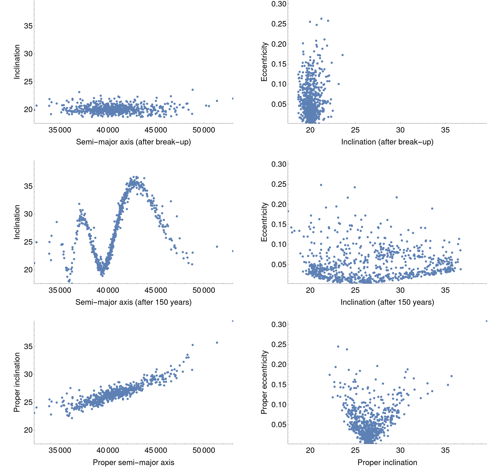
Figure 10. Distribution of $a$-$i$ (left), $i$-$e$ (right) with the parent body at the initial position $a=40600$ km, $e=0.01$, $i=20^{o}$, $\omega=170^{o}$, $\Omega=210^{o}$ after break-up (first row), after 150 years (second row), and proper elements computed after 150 years (third row).

Using the same approach as for the 2:1 resonance, we make an experiment very close to the 1:1 resonance, taking $a=40600$ km, $e=0.01$, $i=20^{o}$, $\omega=170^{o}$, $\Omega=210^{o}$. In total, 815 fragments have been produced from a collision between a 1300 kg parent body and a 6 kg projectile at the relative velocity of 4900 m/s.

The distributions of proper eccentricity and proper inclination are closer to the original distributions of the fragments, than the distributions obtained using the mean elements. As we already mentioned for the 2:1 resonance, we believe that the whole procedure requires more work and might be improved by using an appropriate resonant normal form procedure.

6. Data analysis, SRP, Noisy data, Constancy over time

In this Section, we aim at supporting the results obtained in the previous Sections by analyzing different aspects:

• we use statistical data analysis to quantify the similarities of the distributions of the fragments (see Section 6.1);

• we analyze the effect of Solar radiation pressure (see Section 6.2);

• we make some experiments to study how the distributions are affected by noise (see Section 6.3);

• we provide some experiments to see the dependence of the results on the propagation time (see Section 6.4).

6.1. Data analysis of the results

In this Section we implement statistical methods for data analysis ([3], [16]) to quantify the links between the distributions of osculating, mean and proper elements. As in the previous Sections, we compare the distributions of semimajor axis, eccentricity and inclination at break-up, after 150 years, and by computing the proper elements after 150 years.

Our procedure relies on the following steps: (S1) we use histograms to check the distributions of the data, (S2) we scan the datasets to find possible outliers, (S3) we perform the Kolmogorov-Smirnov (K-S) test to compare the distributions, and finally (S4) we compute the Pearson correlation coefficient between the datasets (see Appendix B for further details on each step of the procedure and the relevant definitions).

As an example, we take the case of moderate orbits presented in Figure 4 and we implement the above steps (S1)-(S4) to analyze the data. Since the semi-major axis is always constant, we are interested just in the analysis of eccentricity and inclination.

In Figure 11 we show the histograms of $e$ and $i$ (step (S1)) in three situations: initial distribution, mean elements distribution (after 150 years), and proper elements distribution (after 150 years). The right plot of Figure 11 shows the inclinations: the initial and proper inclinations have the same shape and size, although they are shifted; the mean inclination curve has instead different shape and size, thus underlining (once more) the different behavior of the mean elements with respect to the initial ones. As for the eccentricity given in the left plot of Figure 11, all curves are almost overlapping, since the forces (geopotential, Sun and Moon) do not affect too much the evolution of the eccentricity, since we are taking the initial data in a stable region far from the tesseral and lunisolar resonances.

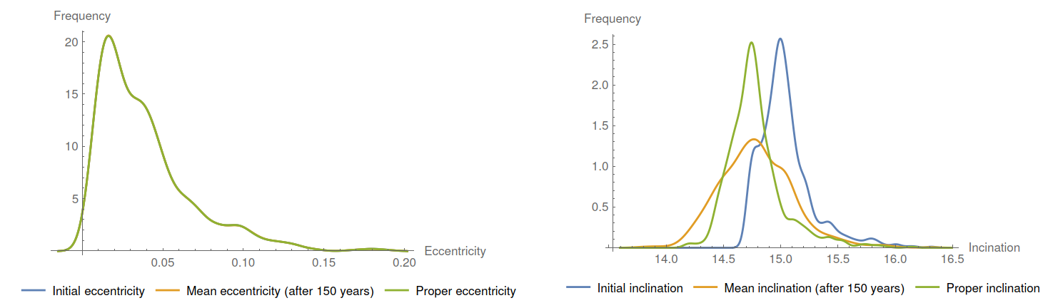
Figure 11. Histograms of $e$ (left) and $i$ (right) for a parent body with orbital elements $a=20600$ km, $e=0.01$, $i=15^{o}$, $\omega=10^{o}$, $\Omega=20^{o}$.

As for step (S2), while checking the outliers for this experiment, we found 2 anomalies in the dataset of the initial semi-major axis; however, only one of them is preserved for the mean and proper semi-major axes. As for the eccentricity, we found 4 outliers in the initial dataset; 3 of them are also found in the proper eccentricity set, while for the mean eccentricity we found 3 more outliers. Concerning the inclination, we have 3 outliers in the initial data, 7 in the final mean dataset, and 6 in the proper inclination set. The conclusion is that the number of outliers is very small for each dataset and it does not affect the performance of the other statistical tests (e.g., Pearson correlation and the K-S test).

The behaviour of the distributions is confirmed also by the K-S test (step (S3)), which gives a small p-value equal to $0.0015$ when checking the similarity between the initial dataset and the mean elements after 150 years, while it gives a higher p-value equal to $0.5167$ when looking at the initial data and the proper elements (see Table 3).

Step (S4) provides evidence of the difference in inclination between the initial data and the data after 150 years; this is obtained by computing the Pearson correlation coefficient which turns out to be equal to $0.7423$. Instead, a higher coefficient equal to $0.9720$ is obtained when comparing the initial and proper elements.

We summarize in Table 3 the results of the data analysis of the different samples studied in the previous sections; the samples can be identified through the semi-major axis.

6.2. The effect of Solar radiation pressure (SRP)

Solar radiation pressure affects mostly the fragments with high area-to-mass ($A/m$) ratio. Since the break-up simulator returns the $A/m$ ratio for each fragment, we perform also a test on the computation of the proper elements including SRP. Following [23], we use (2.7) to model SRP; the explicit expression is given in Appendix C.

Since the Hamiltonian in Appendix C depends also on the angle $M_{S}$, we treat the new angle as we did it for the ascending node of the Moon, namely we introduce a dummy variable associated to $M_{S}$ which gives a 5 degrees of freedom Hamiltonian system. The normalization algorithm then follows the same steps as described in Section 4.1.

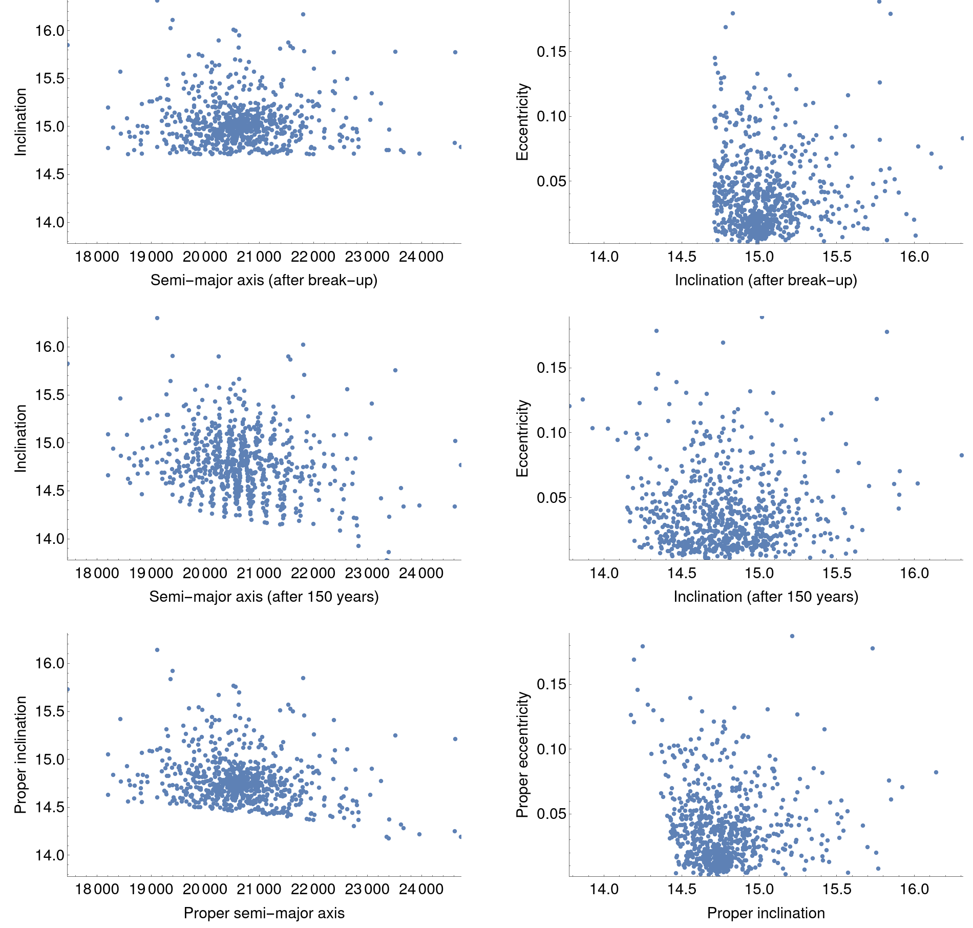
Figure 12. Distribution of $a$-$i$ (left), $i$-$e$ (right) for a parent body with orbital elements $a=20600$ km, $e=0.01$, $i=15^{o}$, $\omega=10^{o}$, $\Omega=20^{o}$ after break-up (first row), after 150 years (second row), and proper elements computed after 150 years (third row). Additional effect: SRP.

The results provided in Figure 12 reproduce those of Figure 4 with the addition of SRP, which is computed by the simulator for each fragment; the values of the area-to-mass ratio range from $A/m=0.05$ to $A/m=0.74$. Since such values are not too large, there are not big differences between Figure 4 and Figure 12. Indeed, we notice only a small difference in the computation of the Pearson correlation coefficients between the initial and mean elements ($0.742391$), and initial and proper elements ($0.932413$). For all other experiments described in the previous Sections, the values of the Pearson coefficient and the K-S test p-value are provided in Table 3.

6.3. Proper elements and random noise

To complement the previous results, we add a simple experiment to take into account the behaviour of proper elements in case of noisy initial conditions. We believe that this topic deserves a thorough study; however, we think interesting to give a preliminary insight on a test sample, following this procedure: consider the evolution of the mean elements starting from some initial values, add noise to the latter, and then compute the proper elements using the noisy data.

The noise is introduced by computing the orbital elements according to the following formulae: $a_{N}=a(1+0.001\tau)$, $e_{N}=e(1+0.05\tau)$, $i_{N}=i(1+0.005\tau)$, $M_{N}=M(1+0.005\tau)$, $\omega_{N}=\omega(1+0.005\tau)$, $\Omega_{N}=\Omega(1+0.005\tau)$, where $\tau$ is a random number taking the values -1, 0, or 1.

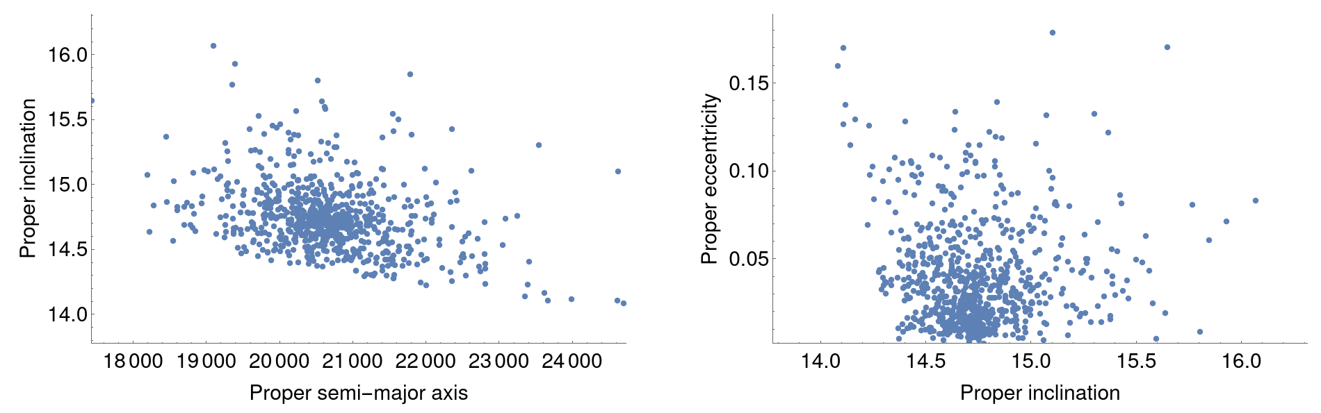
Figure 13. Distribution of $a$-$i$ (left), $i$-$e$ (right) with the parent body at the initial position $a=20600$ km, $e=0.01$, $i=15^{o}$, $\omega=10^{o}$, $\Omega=20^{o}$: proper elements computed after 150 years. Additional effect: random noise.

Again, we consider the sample already presented in Figure 4, but adding noise. The results show a larger spread with respect to the case without noise as shown in Figure 13, and comparing the histogram from Figure 11 and Figure 14. The conclusion of such experiment is that adding a small noise to the orbital elements, we are still able to reproduce the initial distributions with a fairly good approximation. A result which is confirmed also by the values of the statistical tests reported in Table 3.

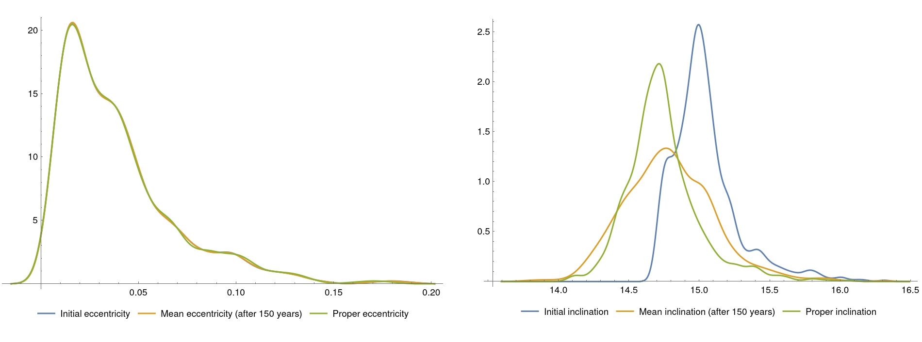
Figure 14. Histogram of $e$ (left) and $i$ (right) for e parent body at the initial position $a=20600$ km, $e=0.01$, $i=15^{o}$, $\omega=10^{o}$, $\Omega=20^{o}$. Additional effect: random noise.

6.4. Constancy of the proper elements

Using the results obtained in Section 4.3, we analyze how the distribution of the proper elements changes when we take different evolution times. To this end, we consider the fragments at four different times: 0 years, 50 years, 100 years and 150 years. For each time and each fragment, we obtain a set of final data from which we compute the proper elements; for this reason, we will refer to the time at which we compute the proper elements as the proper-time. The results are given in Figure 15. The plots make clear that the mean elements distributions change with time, while those of the proper elements are kept nearly constant; this fact is reflected also by the statistical data analysis shown in Figure 15, namely by the histograms and the values of the Pearson correlation coefficients.

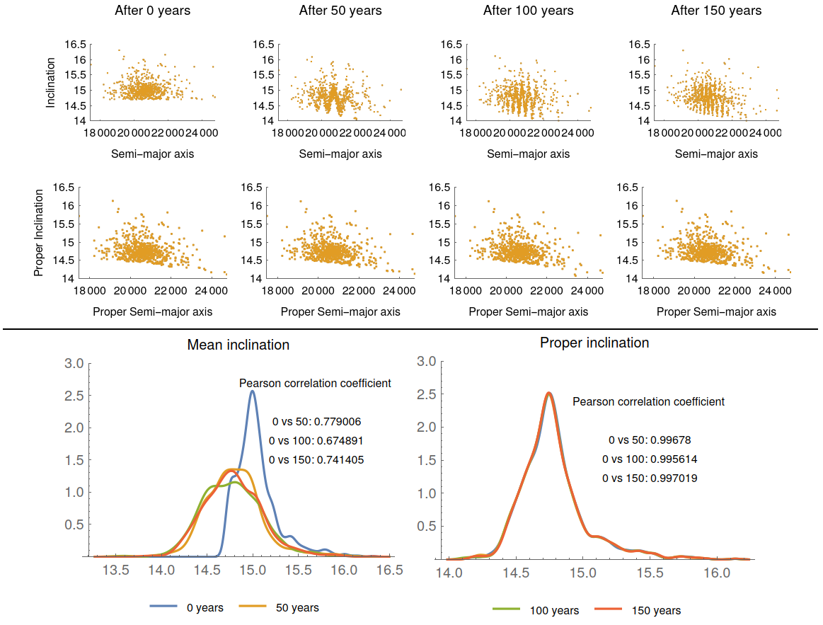
Figure 15. Comparison of mean inclination and proper inclination at different times 0 years, 50 years, 100 years, 150 years (top). Distribution and Pearson correlation coefficient for mean inclination (bottom-left) and for proper inclination (bottom-right).

7. Conclusions and further work

In the present paper we developed a method to compute proper elements for groups of fragments of space debris associated to the same break-up event. The Hamiltonian formulation of the model was adopted to describe the dynamics taking into account three main forces: the potential of the Earth, and the attraction of the Moon and the Sun. We also make some experiments to evaluate the effect of Solar radiation pressure and that of data affected by noise. Using a break-up simulator reproducing the model described in [24], we analyzed the effectiveness of the computation of the proper elements in different regions, which include moderate altitude orbits ($a=15100$ km and $a=20600$ km), and medium altitude orbits ($a=33600$ km). The experiments consisted in a comparison of the distribution of the elements $a,e,i$ in three different scenarios: after break-up, after 150 years and after the transformation into proper elements of the data propagated to 150 years. The main results come from the plots in Sections 4.3, 4.4. The plots obtained computing the proper elements show a distribution similar to that after the break-up; the results are supported by data analysis, mainly through histograms, the K-S test and the determination of the Pearson correlation coefficient. We have also noticed that the proper elements become very useful when analyzing the dynamics after long periods of time. Indeed, we can use them as a prediction of the mean position of the group of fragments using the information at the break-up time.

We also included a computation of proper elements in the neighborhood of the 1:1 and 2:1 tesseral resonances. Although the present results display already the correct behaviour, we believe that the resonant cases need a more accurate investigation and their analysis can be improved through the development of a resonant normalization procedure.

Our conclusion is that the present work should be seen as a proof of the conceptual relevance of normal forms and proper elements in classifying space debris, especially when associated to break-up events, either an explosion or a collision between two satellites. Some real cases have been successfully studied in [14], using some of the methods detailed in the present work. In view of possible applications, we foresee several ways to improve the results, in primis the study of a more elaborated model including a larger number of spherical harmonics and a higher order expansion of the Hamiltonian. Another ingredient that can contribute to improve the results is to push the normalization procedure to higher orders. Besides, we believe that it could be worth investigating the effectiveness of synthetic versus analytic proper elements. As a further direction of our work, we plan to explore the construction and use of approximate integrals within the LEO region, in which the objects are affected by the atmospheric drag. The dissipative effect in LEO might require to develop tools different than those presented in this work.

Semi-major axis	Additional effect	K-S p-value inclination after 150 years	K-S p-value proper inclination	Pearson coefficient inclination after 150 years	Pearson coefficient proper inclination
	None	$0.000157468$	$0.504867$	$0.683247$	$0.99892$
$15100$ km	SRP	$0$	$0$	$0.397109$	$0.42841$
	Noise	$0.000157468$	$0.00403839$	$0.683247$	$0.872222$
	None	$0.00158629$	$0.516702$	$0.742373$	$0.972032$
$20600$ km	SRP	$0.691085$	$0.910099$	$0.742391$	$0.932413$
	Noise	$0.00158629$	$0.223151$	$0.742373$	$0.924797$
	None	$0.00543351$	$0.994865$	$0.731604$	$0.999159$
$24600$ km (2 groups)	SRP	$0.00405436$	$0.994865$	$0.738282$	$0.999185$
	Noise	$0.00543351$	$0.994865$	$0.731604$	$0.987192$
	None	$0.0137999$	$0.999994$	$0.856875$	$0.999546$
$24600$ km (3 groups)	SRP	$0.0203053$	$0.999993$	$0.862371$	$0.999562$
	Noise	$0.0137999$	$0.968287$	$0.856875$	$0.994158$
	None	$0.188238$	$0.999855$	$0.126101$	$0.997886$
$26600$ km	SRP	$0.159541$	$0.81169$	$0.126514$	$0.786289$
	Noise	$0.188238$	$0.910099$	$0.126101$	$0.908531$
	None	$0.445528$	$0.945333$	$0.22445$	$0.942989$
$33600$ km	SRP	$0.445528$	$0.945333$	$0.22445$	$0.942989$
	Noise	$0.447331$	$0.447331$	$0.226055$	$0.837718$
	None	$0$	$0.165985$	$0.0272665$	$0.36087$
$40600$ km	SRP	$0$	$0.0902647$	$0.0186929$	$0.349326$
	Noise	$0$	$0$	$0.0680719$	$0.269618$

Table 3. The values for K-S test and Pearson correlation coefficient, obtained by comparing mean and proper elements with the initial data.

Appendix A - Cartesian equations of motion

Let us consider a body orbiting around the Earth. We assume that it is subject to the gravitational attraction of the Earth, which we consider as an extended body, the Moon, and the Sun. We consider two reference systems, with origin in the center of the Earth:

1. a quasi-inertial frame, where the unit vectors $\{\underline{e}_{1},\underline{e}_{2},\underline{e}_{3}\}$ are fixed;

2. a co-rotating frame $\{\underline{f}_{1},\underline{f}_{2},\underline{f}_{3}\}$, in which the Earth is fixed and $\underline{f}_{3}$ is aligned with the spin axis, which rotates at a constant rate $\omega$.

Let $\underline{r}$ be the position of the body, which can be written in both reference systems as

$$\begin{split}\underline{r}&=x\underline{e}_{1}+y\underline{e}_{2}+z\underline{e}_{3}\\ &=X\underline{f}_{1}+Y\underline{f}_{2}+Z\underline{f}_{3}\ .\end{split}$$

Denoting by $\theta$ the sidereal time, the relation between the coordinates $(x,y,z)$ and $(X,Y,Z)$ is given by

$$\begin{pmatrix}x\\ y\\ z\end{pmatrix}=R_{3}(-\theta)\begin{pmatrix}X\\ Y\\ Z\end{pmatrix},$$

where

$$R_{3}(\theta)=\begin{pmatrix}\cos\theta&-\sin\theta&0\\ \sin\theta&\cos\theta&0\\ 0&0&1\\ \end{pmatrix}.$$

Let $\underline{r}_{S},\underline{r}_{M}$ be the positions of the Sun and the Moon with respect to the center of the Earth, $m_{S}$, $m_{M}$ the masses of the Sun and the Moon, and $\mathcal{G}$ the gravitational constant. The Cartesian equations of motion for a satellites in orbit around the Earth are written as

$$\begin{split}\ddot{\underline{r}}=&-\mathcal{G}\int_{{\mathcal{V}_{E}}}\rho(\underline{r}_{p})\frac{\underline{r}-\underline{r}_{p}}{\lvert\underline{r}-\underline{r}_{p}\rvert^{3}}d{\mathcal{V}_{E}}-\mathcal{G}m_{S}\bigg{(}\frac{\underline{r}-\underline{r}_{S}}{\lvert\underline{r}-\underline{r}_{S}\rvert^{3}}+\frac{\underline{r}_{S}}{\lvert\underline{r}_{S}\rvert^{3}}\bigg{)}\\ &-\mathcal{G}m_{M}\bigg{(}\frac{\underline{r}-\underline{r}_{M}}{\lvert\underline{r}-\underline{r}_{M}\rvert^{3}}+\frac{\underline{r}_{M}}{\lvert\underline{r}_{M}\rvert^{3}}\bigg{)},\end{split}$$ (7.1)

where ${\mathcal{V}_{E}}$ is the volume of the Earth, $\underline{r}_{p}$ is the position vector of a point inside the Earth, $\rho(\underline{r}_{p})$ denotes the density at $\underline{r}_{p}$; the other two terms in (7.1) represent the gravitational attraction of Sun and Moon, respectively. Denoting by

$$V(\underline{r})=\mathcal{G}\int_{\mathcal{V}_{E}}\frac{\rho(\underline{r}_{p})}{\lvert\underline{r}-\underline{r}_{p}\rvert}d\mathcal{V}_{E}$$

the gravitational potential of the Earth and with $\nabla_{\underline{f}}$ the gradient with respect to the co-rotating frame, the first term at the right hand side of (7.1) can be written as

$$R_{3}(-\theta)\nabla_{\underline{f}}V(\underline{r}).$$ (7.2)

A.1 Spherical harmonics expansion of the geopotential

The Earth’s gravitational potential can be expanded as a series of spherical harmonics ([25]). Let us introduce spherical coordinates in the co-rotating frame as

$$\begin{cases}X=r\cos\phi\cos\lambda,\\ Y=r\cos\phi\sin\lambda,\\ Z=r\sin\phi,\\ \end{cases}$$

where $0\leq\lambda<2\pi$, $-\frac{\pi}{2}\leq\phi<\frac{\pi}{2}$. The series expansion of $V$ in spherical harmonics is given by

$$V(r,\phi,\lambda)=\frac{\mathcal{G}m_{E}}{r}\sum_{n=0}^{\infty}\bigg{(}\frac{R_{E}}{r}\bigg{)}^{n}\sum_{m=0}^{n}P_{nm}(\sin\phi)\big{[}C_{nm}\cos(m\lambda)+S_{nm}\sin(m\lambda)\big{]}.$$

Here, the functions $P_{nm}$ are defined in terms of the Legendre polynomials $P_{n}(x)$ as

$$P_{nm}(x)=(1-x^{2})^{m/2}\frac{d^{m}}{dx^{m}}P_{n}(x),$$

and $C_{nm},S_{nm}$ are the harmonic coefficients obtained by the following formulae:

$$C_{nm}=\frac{2-\delta_{0m}}{m_{E}}\frac{(n-m)!}{(n+m)!}\int_{{\mathcal{V}_{E}}}(\frac{r_{p}}{R_{e}})^{n}P_{nm}(\sin\phi_{p})\cos(m\lambda_{p})\rho(\underline{r}_{p})d{\mathcal{V}_{E}}$$

$$S_{nm}=\frac{2-\delta_{0m}}{m_{E}}\frac{(n-m)!}{(n+m)!}\int_{{\mathcal{V}_{E}}}(\frac{r_{p}}{R_{e}})^{n}P_{nm}(\sin\phi_{p})\sin(m\lambda_{p})\rho(\underline{r}_{p})d{\mathcal{V}_{E}}\ ,$$

where $m_{E}$ is the mass of the Earth, $(r_{p},\phi_{p},\lambda_{p})$ denote the spherical coordinates associated to a point $P$ inside the Earth and, again, $r_{p}$ is its radius vector ($\delta_{jm}$ is the Kronecker symbol).

The coefficients $C_{nm}$ and $S_{nm}$ are related to the quantities $J_{nm}$ and $\lambda_{nm}$ of Table 1 by

$$J_{nm} = (C_{nm}^{2}+S_{nm}^{2})^{1\over 2}\qquad{\rm for}\ m\not=0\ ,$$

$$J_{n0} = J_{n}=-C_{n0}\quad\ \qquad{\rm for}\ m=0\ .$$

A.2 Equations of motion up to 2nd order

The Cartesian equations of motion in the quasi-inertial reference frame are given by the rotation (7.2) and by computing the partial derivatives of the potential with respect to spherical coordinates:

$$R_{3}(-\theta)\nabla_{\underline{f}}V(\underline{r})=\big{(}\frac{\partial V}{\partial X}\cos\theta-\frac{\partial V}{\partial Y}\sin\theta\big{)}\underline{e}_{1}+\big{(}\frac{\partial V}{\partial X}\sin\theta+\frac{\partial V}{\partial Y}\cos\theta\big{)}\underline{e}_{2}+\frac{\partial V}{\partial Z}\underline{e}_{3}\ ,$$ (7.3)

where the potential up to order $n=m=2$ in the co-rotating frame is given by

$$V(X,Y,Z)=\frac{\mathcal{G}m_{E}}{r}+\frac{\mathcal{G}m_{E}}{r}(\frac{R_{E}}{r})^{2}\big{[}C_{20}\big{(}\frac{3Z^{2}}{2r^{2}}-\frac{1}{2}\big{)}+3C_{22}\frac{X^{2}-Y^{2}}{r^{2}}+6S_{22}\frac{XY}{r^{2}}\big{]}\ .$$

By differentiating the potential $V$ with respect to $X,Y,Z$ and substituting the result in (7.3) and (7.1), we find the following expression for the Cartesian equations of motion:

$$\begin{split}\ddot{x}=&-\frac{\mathcal{G}m_{E}x}{r^{3}}+\frac{\mathcal{G}m_{E}R_{E}^{2}}{r^{5}}\left\{C_{20}\big{(}\frac{3}{2}x-\frac{15}{2}\frac{xz^{2}}{r^{2}}\big{)}+6C_{S}^{-}x+6C_{S}^{+}y\right.\\ &\left.+\frac{15x}{r^{2}}[C_{S}^{-}(y^{2}-x^{2})-2xyC_{S}^{+}]\right\}-\mathcal{G}m_{S}\bigg{(}\frac{x-x_{S}}{\lvert\underline{r}-\underline{r}_{S}\rvert^{3}}+\frac{x_{S}}{\lvert x_{S}\rvert^{3}}\bigg{)}\\ &-\mathcal{G}m_{M}\bigg{(}\frac{x-x_{M}}{\lvert\underline{r}-\underline{r}_{M}\rvert^{3}}+\frac{x_{M}}{\lvert\underline{r}_{M}\rvert^{3}}\bigg{)},\end{split}$$

$$\begin{split}\ddot{y}=&-\frac{\mathcal{G}m_{E}y}{r^{3}}+\frac{\mathcal{G}m_{E}R_{E}^{2}}{r^{5}}\left\{C_{20}\big{(}\frac{3}{2}y-\frac{15}{2}\frac{yz^{2}}{r^{2}}\big{)}+6C_{S}^{+}x-6C_{S}^{-}y\right.\\ &\left.+\frac{15y}{r^{2}}[C_{S}^{-}(y^{2}-x^{2})-2xyC_{S}^{+}]\right\}-\mathcal{G}m_{S}\bigg{(}\frac{y-y_{S}}{\lvert\underline{r}-\underline{r}_{S}\rvert^{3}}+\frac{y_{S}}{\lvert\underline{r}_{S}\rvert^{3}}\bigg{)}\\ &-\mathcal{G}m_{M}\bigg{(}\frac{y-y_{M}}{\lvert\underline{r}-\underline{r}_{M}\rvert^{3}}+\frac{y_{M}}{\lvert\underline{r}_{M}\rvert^{3}}\bigg{)},\end{split}$$

$$\begin{split}\ddot{z}=&-\frac{\mathcal{G}m_{E}z}{r^{3}}+\frac{\mathcal{G}m_{E}R_{E}^{2}}{r^{5}}\left\{C_{20}\big{(}\frac{9}{2}z-\frac{15}{2}\frac{z^{3}}{r^{2}}\big{)}+\frac{15z}{r^{2}}[C_{S}^{-}(y^{2}-x^{2})-2xyC_{S}^{+}]\right\}\\ &-\mathcal{G}m_{S}\bigg{(}\frac{z-z_{S}}{\lvert\underline{r}-\underline{r}_{S}\rvert^{3}}+\frac{z_{S}}{\lvert\underline{r}_{S}\rvert^{3}}\bigg{)}-\mathcal{G}m_{M}\bigg{(}\frac{z-z_{M}}{\lvert\underline{r}-\underline{r}_{M}\rvert^{3}}+\frac{z_{M}}{\lvert\underline{r}_{M}\rvert^{3}}\bigg{)}\ ,\end{split}$$

where $C_{S}^{+}=C_{22}\sin 2\theta+S_{22}\cos 2\theta$, $C_{S}^{-}=C_{22}\cos 2\theta-S_{22}\sin 2\theta$.

Appendix B - Data Analysis

In this Section we report the basic elements of data analysis, used in the rest of this work to get useful information from the dataset associated to the fragments. We refer to [3], [16] for further details.

B.1 Histogram

To visualize the data and to understand the main features of a distribution, one can plot the histogram of the dataset. This plot shows the frequency of each element from the set. It turns out to be a useful tool to compare the distributions of two or more data sets.

B.2 Outliers

Outliers are rare data points far away from regular data points and generally do not form a tight cluster. To check them, we count the anomalies in each dataset of semi-major axis, eccentricity, and inclination in all three situations: initial osculating elements, final mean elements, and proper elements. We used a predefined Mathematica^© function, $FindAnomalies$ from the $MachineLearning$ package, which is computed as:

$$p=\mathbb{P}(f_{\mathcal{D}}(y)\leq f_{\mathcal{D}}(x),y\approx\mathcal{D})\ ,$$

where $\mathbb{P}$ denotes the probability, $\mathcal{D}$ is the approximated distribution of a 1D array $X$, $x$ is an element in $X$ and $f_{\mathcal{D}}(x)$ is the probability density function of $\mathcal{D}$; $y\approx\mathcal{D}$ means that $y$ follows the distribution $\mathcal{D}$. In case of $p<0.001$ (default threshold), $FindAnomalies$ considers $x$ as anomalous. This function returns the number of outliers, the value of each outlier, and its position in the dataset. With this information, we can compare the outliers for osculating, mean and proper elements.

B.3 Pearson correlation coefficient

Pearson correlation coefficient, usually denoted by $r$, is used as a statistical measurement of the relationship between two one-dimensional datasets. Mathematically, it is a real number in $[-1,1]$, where $1$ means a total positive linear relationship, $0$ means no relationship, and $-1$ means a total negative linear relationship between the two datasets.

For two variables (1D arrays) $X=(x_{1},\dots,x_{n}),Y=(y_{1},\dots,y_{n})$, we define the following statistical measures:

1. Mean of $X$: $\bar{X}=\frac{1}{n}\sum_{i=1}^{n}x_{i}$

2. Variance of $X$: $Var[X]=\frac{1}{n-1}\sum_{i=1}^{n}(x_{i}-\bar{X})$

3. Covariance of $X$ and $Y$: $Cov[X,Y]=\frac{1}{n-1}\sum_{i=1}^{n}(x_{i}-\bar{X})(y_{i}-\bar{Y})$ .

Then, the Pearson correlation coefficient is defined as

$$r=\frac{Cov[X,Y]}{Var[X]Var[Y]}\ .$$

B.4 Kolmogorv-Smirnov test

Kolmogorov-Smirnov test is a goodness-of-fit test where the null hypothesis says that two datasets are drawn from the same distribution and the alternative hypothesis that they were not drawn from the same distribution.

Appendix C - Solar radiation pressure

Here we give the full expression of the Solar radiation pressure Hamiltonian, starting from the expression (2.7):

$$\mathcal{H}_{SRP}=a\frac{A}{m}\left(\left(-1.1446\times 10^{-10}\right)e\cos\left(-\omega-\Omega-M_{S}+4.9382\right)\right.\\ \left.-\left(1.1446\times 10^{-10}\right)e\cos(i)\cos\left(-\omega-\Omega-M_{S}+4.9382\right)-\left(1.1446\times 10^{-10}\right)e\cos\left(\omega-\Omega-M_{S}+4.9382\right)\right.\\ \left.+\left(1.1446\times 10^{-10}\right)e\cos(i)\cos\left(\omega-\Omega-M_{S}+4.9382\right)-\left(3.2784\times 10^{-6}\right)e\cos\left(-\omega-\Omega+M_{S}+4.9382\right)\right.\\ \left.-\left(3.2784\times 10^{-6}\right)e\cos(i)\cos\left(-\omega-\Omega+M_{S}+4.9382\right)-\left(3.2784\times 10^{-6}\right)e\cos\left(\omega-\Omega+M_{S}+4.9382\right)\right.\\ \left.+\left(3.2784\times 10^{-6}\right)e\cos(i)\cos\left(\omega-\Omega+M_{S}+4.9382\right)-\left(1.4109\times 10^{-7}\right)e\cos\left(-\omega+\Omega+M_{S}+4.9382\right)\right.\\ \left.+\left(1.4109\times 10^{-7}\right)e\cos(i)\cos\left(-\omega+\Omega+M_{S}+4.9382\right)-\left(1.4109\times 10^{-7}\right)e\cos\left(\omega+\Omega+M_{S}+4.9382\right)\right.\\ \left.-\left(1.4109\times 10^{-7}\right)e\cos(i)\cos\left(\omega+\Omega+M_{S}+4.9382\right)-\left(1.0959\times 10^{-7}\right)e\cos\left(-\omega-\Omega+2M_{S}+4.9382\right)\right.\\ \left.-\left(1.0959\times 10^{-7}\right)e\cos(i)\cos\left(-\omega-\Omega+2M_{S}+4.9382\right)-\left(1.0959\times 10^{-7}\right)e\cos\left(\omega-\Omega+2M_{S}+4.9382\right)\right.\\ \left.+\left(1.0959\times 10^{-7}\right)e\cos(i)\cos\left(\omega-\Omega+2M_{S}+4.9382\right)-\left(4.7161\times 10^{-9}\right)e\cos\left(-\omega+\Omega+2M_{S}+4.9382\right)\right.\\ \left.+\left(4.7161\times 10^{-9}\right)e\cos(i)\cos\left(-\omega+\Omega+2M_{S}+4.9382\right)-\left(4.7161\times 10^{-9}\right)e\cos\left(\omega+\Omega+2M_{S}+4.9382\right)\right.\\ \left.-\left(4.7161\times 10^{-9}\right)e\cos(i)\cos\left(\omega+\Omega+2M_{S}+4.9382\right)-\left(3.0904\times 10^{-9}\right)e\cos\left(-\omega-\Omega+3M_{S}+4.9382\right)\right.\\ \left.-\left(3.0904\times 10^{-9}\right)e\cos(i)\cos\left(-\omega-\Omega+3M_{S}+4.9382\right)-\left(3.0904\times 10^{-9}\right)e\cos\left(\omega-\Omega+3M_{S}+4.9382\right)\right.\\ \left.+\left(3.0904\times 10^{-9}\right)e\cos(i)\cos\left(\omega-\Omega+3M_{S}+4.9382\right)-\left(1.3299\times 10^{-10}\right)e\cos\left(-\omega+\Omega+3M_{S}+4.9382\right)\right.\\ \left.+\left(1.3299\times 10^{-10}\right)e\cos(i)\cos\left(-\omega+\Omega+3M_{S}+4.9382\right)-\left(1.3299\times 10^{-10}\right)e\cos\left(\omega+\Omega+3M_{S}+4.9382\right)\right.\\ \left.-\left(1.3299\times 10^{-10}\right)e\cos(i)\cos\left(\omega+\Omega+3M_{S}+4.9382\right)-\left(1.3602\times 10^{-6}\right)e\cos\left(-\omega+M_{S}+4.9382\right)\sin(i)\right.\\ \left.+\left(1.3602\times 10^{-6}\right)e\cos\left(\omega+M_{S}+4.9382\right)\sin(i)-\left(4.5468\times 10^{-8}\right)e\cos\left(-\omega+2M_{S}+4.9382\right)\sin(i)\right.\\ \left.+\left(4.5468\times 10^{-8}\right)e\cos\left(\omega+2M_{S}+4.9382\right)\sin(i)-\left(1.2822\times 10^{-9}\right)e\cos\left(-\omega+3M_{S}+4.9382\right)\sin(i)\right.\\ \left.+\left(1.2822\times 10^{-9}\right)e\cos\left(\omega+3M_{S}+4.9382\right)\sin(i)\right).\\$$ (7.4)

Acknowledgements. The authors thank C. Efthymiopoulos, C. Galeş and D. Marinucci for useful discussions and suggestions. The authors thank the anonymous Reviewers that greatly contributed to improve the content and the presentation of this work. All authors acknowledge EU H2020 MSCA ETN Stardust-R Grant Agreement 813644. A.C. (partially) acknowledges the MIUR Excellence Department Project awarded to the Department of Mathematics, University of Rome Tor Vergata, CUP E83C18000100006. A.C. (partially) and G.P. acknowledge MIUR-PRIN 20178CJA2B “New Frontiers of Celestial Mechanics: theory and Applications”. G.P. acknowledges GNFM/INdAM and is partially supported by INFN (Sezione di Roma II).

Conflict of Interest. The author A.C. is Editor-in-Chief of the journal “Celestial Mechanics and Dynamical Astronomy”; the paper underwent a standard single-blind peer review process.

Data availability. The datasets generated during and/or analysed during the current study are available from the corresponding author on reasonable request.

References

• [1] M. Apetrii, A. Celletti, E. Efthymiopoulos, C. Galeş, G. Pucacco, T. Vartolomei, On a simulator of break-up events for space debris, Work in progress (2021)
• [2] AAVV, NASA Standard break-up Model 1998 Revision, prepared by Lockheed Martin Space Mission Systems $\&$ Services for NASA, July 1998
• [3] S. Brandt, Data analysis, Springer, Cham (2014)
• [4] S. Breiter, Lunisolar resonances revisited, Celest. Mech. Dyn. Astr. 81, 81–91 (2001)
• [5] D. Brouwer, Secular variations of the orbital elements of minor planets, Astron. J. 56, 9-32 (1951)
• [6] D. Casanova, A. Petit, A. Lemaitre, Long-term evolution of space debris under the $J_{2}$ effect, the solar radiation pressure and the solar and lunar perturbations, Celest. Mech. Dyn. Astr. 123, 223–238 (2015)
• [7] A. Celletti, F. Gachet, C. Galeş, G. Pucacco, C. Efthymiopoulos, Dynamical models and the onset of chaos in space debris, Int. J. Nonlinear Mechanics 90, 47-163 (2017)
• [8] A. Celletti, C. Galeş, On the dynamics of space debris: 1:1 and 2:1 resonances, J. Nonlinear Science 24, n. 6, 1231-1262 (2014)
• [9] A. Celletti, C. Galeş, G. Pucacco, Bifurcation of lunisolar secular resonances for space debris orbits, SIAM J. Appl. Dyn. Syst. 15, 1352-1383 (2016)
• [10] A. Celletti, C. Galeş, A study of the lunisolar secular resonance $2\dot{\omega}+\dot{\Omega}=0$, Front. Astron. Space Sci. - Fundamental Astronomy, 31 March 2016
• [11] A. Celletti, C. Galeş, Dynamics of resonances and equilibria of Low Earth Objects, SIAM J. Appl. Dyn. Syst. 17, 203-235 (2018)
• [12] A. Celletti, C. Galeş, G. Pucacco, A. Rosengren, Analytical development of the lunisolar disturbing function and the critical inclination secular resonance, Celest. Mech. Dyn. Astron. bf 127, n. 3, 259-283 (2017)
• [13] A. Celletti, C. Galeş, C. Lhotka, Resonance in the Earht’s space environment, Nonlinear Sc. Num. Sim. 84, 105185 (2020)
• [14] A. Celletti, G. Pucacco, T. Vartolomei, Reconnecting groups of space debris to their parent body through proper elements, Nature Scientific Reports 11, 22676 (2021)
• [15] C. Efthymiopoulos, Canonical perturbation theory, stability and difusion in Hamiltonian systems: applications in dynamical astronomy, Workshop Series of the Asociacion Argentina de Astronomia 3, 3-146 (2011)
• [16] G. Cowan, Statistical data analysis, Oxford University Press (1998)
• [17] Deprit, A., & Rom, A.. The main problem of artificial satellite theory for small and moderate eccentricities. Celestial Mechanics, 2(2), 166–206 (1970).
• [18] Earth Gravitational Model 2008, $http://earth-info.nga.mil/GandG/wgs84/gravitymod/egm2008/$
• [19] T.A. Ely, K.C. Howell, Dynamics of artificial satellite orbits with tesseral resonances including the effects of luni-solar perturbations, Dynamics and Stability of Systems 12, n. 4, 243-269 (1997)
• [20] F. Gachet, A. Celletti, G. Pucacco, C. Efthymiopoulos, Geostationary secular dynamics revisited: application to high area-to-mass ratio objects, Celest. Mech. Dyn. Astr. 128, n.2-3, 149-181 (2017)
• [21] I. Gkolias, C. Colombo, Towards a sustainable exploitation of the geosynchronous orbital region, Celest. Mech. Dyn. Astr. 131, n. 19 (2019)
• [22] K. Hirayama, Groups of asteroids probably of common origin, Astron. J. 31, 185-188 (1918)
• [23] S. Hughes, Earth satellite orbits with resonant lunisolar perturbations. I. Resonances dependent only on inclination, Proc. R. Soc. Lond. A 372, 243–264 (1980)
• [24] N. L. Johnson, P. H. Krisko, J.-C. Lieu, and P. D. Am-Meador, NASA’s new break-up model of EVOLVE 4.0, Adv. Space Res. 28, n. 9, 1377-1384 (2001)
• [25] W.M. Kaula, Theory of Satellite Geodesy, Blaisdell Publ. Co. (1966)
• [26] W.M. Kaula, Development of the lunar and solar disturbing functions for a close satellite, Astron. J. 67, 300-303 (1962)
• [27] H. Klinkrad, Space Debris: Models and Risk Analysis, Springer-Praxis, Berlin-Heidelberg (2006)
• [28] Z. Knežević, Asteroid Family Identification: History and State of the Art, Proceedings IAU Symposium No. 318, 2015, S. R. Chesley, A. Morbidelli, R. Jedicke, D. Farnocchia, eds., International Astronomical Union (2016)
• [29] Z. Knežević, A. Lemaitre, A. Milani, The Determination of Asteroid Proper Elements, in Asteroids III, ed.W. Bottke et al. (Tucson: Arizona Univ. Press and LPI), 603 (2003)
• [30] Z. Knežević, A. Milani, Synthetic proper elements for outer main belt asteroids, Celest. Mech. Dyn. Astron. 78, 17-46 (2000)
• [31] Z. Knežević, A. Milani, Proper element catalogs and asteroid families, Astron. Astrophys. 403, 1165-1173 (2003)
• [32] Z. Knežević, A. Milani, Are the analytical proper elements of asteroids still needed?, Celest. Mech. Dyn. Astron. 131, 27 (2019)
• [33] Y. Kozai, The dynamical evolution of the Hirayama family, in : “Asteroids” (T. Gehrels, Ed.), Univ. Arizona Press, pp. 334-35 (1979)
• [34] A. Lemaitre, Proper Elements: What are They?, Celest. Mech. Dyn. Astron. 56, 103-119 (1992)
• [35] A. Lemaitre, A. Morbidelli, Proper elements for highly inclined asteroidal orbits, Celest. Mech. Dyn. Astron. 60, 29-56 (1994)
• [36] C. Lhotka, A. Celletti, C. Galeş, Poynting-Robertson drag and solar wind in the space debris problem, Mon. Not. Roy. Ast. Soc. 460, 802-815 (2016)
• [37] A. Milani, Z. Knežević, Secular perturbation theory and computation of asteroid proper elements, Mech. Dyn. Astron. 49, 347-411 (1990)
• [38] A. Milani, Z. Knežević, Asteroid proper elements and the dynamical structure of the asteroid main belt, Icarus 107, 219-254 (1994)
• [39] A. Morbidelli, Asteroid secular resonant proper elements, Icarus 105, 48-66 (1993)
• [40] B. Novaković, A. Cellino, Z. Knežević, Families among high-inclination asteroids, Icarus 216, 69-81 (2011)
• [41] H. Poincaré, Les méthodes nouvelles de la mécanique céleste, Gauthier-Villars, 1892-1899
• [42] G. Schettino, E.M. Alessi, A. Rossi, G.B. Valsecchi, A frequency portrait of Low Earth Orbits, Celest. Mech. Dyn. Astron. 131, n. 35 (2019)
• [43] J. Schubart, Additional results on orbits of Hilda-type asteroids, Astron. Astrophys. 241, 297-302 (1991)
• [44] D.K. Skoulidou, A.J. Rosengren, K. Tsiganis, G. Voyatzis, Dynamical lifetime survey of geostationary transfer orbits, Celest. Mech. Dyn. Astron. 130, 77 (2018)
• [45] J.G. Williams, Secular Perturbations in the Solar System, Ph.D. thesis, University of California, Los Angeles (1969)
• [46] M. Yuasa, Theory of secular perturbations of asteroids including terms of higher orders and higher degrees, Publ. Astron. Soc. Jpn. 25, 399 (1973)