Feature Selection for Causal Inference from High Dimensional Observational Data with Outcome Adaptive Elastic Net

Abstract

Feature selection is an extensively studied technique in the machine learning literature where the main objective is to identify the subset of features that provides the highest predictive power. However, in causal inference, our goal is to identify the set of variables that are associated with both the treatment variable and outcome (i.e., the confounders). While controlling for the confounding variables helps us to achieve an unbiased estimate of causal effect, recent research shows that controlling for purely outcome predictors along with the confounders can reduce the variance of the estimate. In this paper, we propose an Outcome Adaptive Elastic-Net (OAENet) method specifically designed for causal inference to select the confounders and outcome predictors for inclusion in the propensity score model or in the matching mechanism. OAENet provides two major advantages over existing methods: it performs superiorly on correlated data, and it can be applied to any matching method and any estimates. In addition, OAENet is computationally efficient compared to state-of-the-art methods.

AND

1 Introduction

In today’s data rich world, we are collecting data on almost every aspect of human activities. Such increasing availability of data is enabling us to discover knowledge and insights that provide an opportunity of making informed decisions in both public and private sectors. While association and model-based prediction help us extract value from data, robust causal inference enables us to identify the effect of potential interventions. Causal inference identifies key insight from data by studying how different actions, treatments, or interventions (or many potential interventions) affect certain desirable outcomes [Stuart, 2010]. Estimating such cause-effect relations is the cornerstone of policy decision making. Moreover, in the case of social studies, healthcare, and medicine, the question of causality is often inevitable. In this paper, we develop novel techniques that helps us generating efficient estimates of causal quantities from large-scale, high-dimensional observational data.

Over the last few decades, methodological advances have improved analytical methods for generating unbiased causal effect estimators from observational data [Rosenbaum et al., 2010]. Matching, more specifically, Propensity Score Matching is one of the most popular methods for identifying causal effect from observational data [Stuart, 2010, Brookhart et al., 2006]. While the usage of propensity score based techniques are increasing in health and social science literature, there is no specific guideline for selecting variables for propensity score model [Brookhart et al., 2006] or other matching methods like Mahalanobis Distance Matching [Rubin, 1979], Coarsened Exact Matching [Iacus et al., 2011], and Mixed Integer Programming Matching [Zubizarreta, 2012]. In addition, researchers often take a “throw in the kitchen sink” approach and control for all available covariates just to make sure that the estimate is free of confounding bias [Shortreed & Ertefaie, 2017]. In support to this practice, in the past, several researchers have claimed that the largest set of observed pre-treatment covariates protects against unobserved confounding. However, recent literature [Shortreed & Ertefaie, 2017, Brookhart et al., 2006, VanderWeele & Shpitser, 2011] show that controlling for all variables may not lead to the expected reduction in bias, even if it includes a sufficient set of confounders. On the other hand, it inflates the variance of the estimate of the causal effect.

1.1 Challenges in Variable Selection for Causal Inference

While taking the parametric approach, causal effect estimation methods mainly consider two statistical models: outcome model and treatment allocation mechanism, both as functions of pre-treatment variables [Ertefaie et al., 2018a]. Variables that appear in both models are regarded as confounders. Inclusion of such variables in the propensity score model or in the matching mechanism ensures an unbiased estimate of the causal quantity considering all such confounders are observed. Ideally, a causal variable selection process must start with the domain knowledge on the underlying treatment allocation mechanism and the predictors of the outcome. Unfortunately, researchers often do not have the access of the expert knowledge, instead, are burdened with a large set of pre-treatment variables. When domain knowledge is available, the expert selection can result a significantly large set of variables and particularly, include pure predictors of treatment and pure predictors of outcome. Moreover, high-dimensional observational data can become challenging to comprehend for an expert and may contain spurious variables that does not have any relation with treatment or outcome.

Altogether, the variable selection for causal effect estimation poses three major problems. First, inclusion of pure treatment predictors and weak confounders that are strongly related to treatment inflate the variance of the estimate, both asymptotically [Rotnitzky et al., 2010] and in finite sample [Brookhart et al., 2006]. In addition, inclusion of such variables can increase bias if the complete set of confounders are not observed [Pearl, 2012, Wooldridge, 2016]. In contrast, selecting the outcomes predictors can enhance the efficiency of the causal estimate [Brookhart et al., 2006, Rotnitzky et al., 2010]. Second, selecting pure treatment predictors increase the possibility of violating the positivity assumption [Stuart, 2010, Schnitzer et al., 2016]. For example, a strong predictor of treatment can have values for which the probability of receiving treatment is almost zero. Selecting that variable can result in estimating zero probability of receiving treatment in finite sample and lead to positivity violation. Schnitzer et al. [2016] call such violation as artificial positivity violation. Finally, inability to discern noise from relevant variable influences the bias and variance of the treatment estimate.

1.2 Relevant Literature

To overcome these challenges, the matching mechanism or the Propensity Score (PS) model should include the confounders (predictors of both outcome and treatment) and pure outcome predictors while eliminating pure treatment predictors and noise. There is a vast literature in machine learning that discusses variable selection for prediction purposes, however, there is little work on identifying variables with the objective discussed above. Bayesian adjustment for confounding (BAC) [Wang et al., 2012] is one of the earliest work in variable selection for causal inference. BAC relies on tuning a parameter representing the odds of a variable that is associated to both outcome and treatment. Wilson & Reich [2014] selects the counfounders using a decision-theoretic approach. First, they select a group of candidate models by utilizing the posterior credible region of parameters that are identified by a fitted Bayesian Regression model. The final model is determined from the candidate set through penalization of models that do not incorporate confounders. However, several simulation studies [Vansteelandt, 2012, Lin et al., 2015] reveal that this approach often includes variables that are only associated with treatment resulting to inflated variance of the causal effect. Motivated by the graphical causal inference framework [Pearl, 2009] and Bayesian model averaging, Talbot et al. [Talbot et al., 2015a] and Talbot and Beaudoin [Talbot & Beaudoin, 2020] proposed a Bayesian causal effect estimation (BCEE) method. In BCEE, posterior probabilities of each model are considered as weights in the averaging process while probabilities are identified from conditional outcome model, given treatment and all observed covariates. However, this approach may exclude weak confounders [Ertefaie et al., 2018a].

Over the years, several researchers proposed machine learning methods to fit either the treatment model [Lee et al., 2010, Westreich et al., 2010, Austin et al., 2013] or the outcome model [Wang et al., 2021]. Brookhart et al. [2006] and Schnitzer et al. [2016] show that such approaches primarily selects variables that are strongly related to either treatment or outcome. Modified penalized regression methods are also utilized in variable selection for causal inference. For instance, Ertefaie et al. [Ertefaie et al., 2018a] used a weighted sum of treatment and outcome model. In addition, they introduced a customized $l_{1}$ penalty function to heavily penalize the treatment predictors. On the other hand, [Shortreed & Ertefaie, 2017] uses an adaptive lasso approach which applies less penalty to the outcome predictors. While [Ertefaie et al., 2018a] improves the small sample properties of outcome regularization, the estimated coefficients do not have any causal interpretation and the parameter selection in [Shortreed & Ertefaie, 2017] is designed solely for Inverse Probability of Treatment Weighted (IPTW) estimator. Moreover, both approaches [Shortreed & Ertefaie, 2017, Ertefaie et al., 2018a] will perform poorly on correlated data due to the inclusion of $l_{1}$ penalty and many causal inference applications, specially in healthcare and medicine, the covariates are highly correlated.

In causal inference with matching method, the variable selection process is followed by sampling process to match the covariate distributions of treated and control groups. The matched counterparts of the treated units in the control group are interpreted as counterfactuals, and the average treatment effect on treated (ATT) is estimated by comparing the outcomes of every matched pair [Stuart, 2010]. One of the popular matching method is the Nearest Neighbor Matching (NNM) [Rubin, 1973, Rosenbaum, 2017] which forms a treated-control pair by matching a treated unit to its nearest control unit based on some prespecified distance metrics. Some commonly used NNM matching methods are Propensity Score Matching (PSM) [Rosenbaum & Rubin, 1983, 1985], Coarsened Exact Matching (CEM) [Iacus et al., 2011], Mahalanobis Distance Matching (MDM) [Rubin, 1979], and Genetic Matching (GM) [Singh & D., ]. In the case of high dimensional data, these widely used NNM methods perform poorly. For instance, PSM projects the covaiate vector space into one dimension disregarding the neighbourhood structure of the dataset, and the matched units in projected dimension often differ on important covariates in actual dimension. MDM is prone to bias in high dimensions since it imposes parametric assumptions, so does the GM. In the presence of large number of covariates, to obtain a good match, CEM discards a lot of samples. In addition, recent results show that the bias of a NNM estimator increases at a rate of $O(N^{-1/p})$ where $N$ is the number of samples and $p$ is is the number of variables [Abadie & Imbens, 2006]. Dimension reduction techniques like Principle Component Analysis (PCA) are commonly have been studied extensively in Machine Learning literature where the main objective is to improve the models’ predictive accuracy by retaining the information content. However, in observational studies using matching methods, the objective is to ensure the local neighborhood structure of the data as a treated sample is essentially matched to a control sample within its locality.

1.3 Contribution

In this paper, we propose a unique modeling framework termed as Outcome Adaptive Elastic Net (OAENet) specifically designed for causal inference to select the confounders and outcome predictors for inclusion in the propensity score model or in the matching mechanism. OAENet provides two major advantages over existing methods: it performs superiorly on correlated data, and it can be applied to any matching methods and any estimates. We compare the performance of the proposed OAENet with state-of-the-art variable selection techniques for causal inference on simulated data. Our preliminary analysis shows that the OAENet achieves less bias, less variance and has better accuracy in selecting variables compared to the benchmark methods. In addition, we plan to develop a policy decision case study from real-world, high dimensional data to show the applicability of the proposed method.

The remainder of the paper is organized as follows. In section 2, we discuss causal inference under potential outcome framework, objective of variable selection problems causal inference, and review adaptive elastic-net. In section 3, we outline the Outcome Adaptive Elastic Net approach. We present the empirical performance of the proposed methods and compare it with alternative approaches on both simulated data in section 4. Finally, we provide the concluding remarks in section 5.

2 Causal Inference from High-dimensional Data

In this section, we provide an overview of causal inference under potential outcome framework, common assumptions, variable selection strategies, and adaptive elastic-net.

2.1 Causality under Potential Outcome Framework

In this paper, we consider the potential outcome framework [Holland, 1986] and matching methods developed under this framework for identifying treatment effect from observational data. In the matching method, an unbiased estimate of causal inference can be achieved if treatment unit $t\in\mathscr{T}$ is exactly matched with a control unit $c\in\mathscr{C}$ in terms of their covariate set $\mathbf{X}\in\mathcal{X}$ [Rosenbaum & Rubin, 1983]. However, in most of the applications, it is impossible to achieve exact matching [Zubizarreta, 2012, Rosenbaum & Rubin, 1983, Nikolaev et al., 2013, King & Nielsen, 2019]. A wide variety of matching methods are employed to make $(t,c)$ pairs (or subset $C\subset\mathscr{C}$ and $T\in\mathscr{T}$) as similar as possible [Zubizarreta, 2012, 2015, Rosenbaum & Rubin, 1983, Nikolaev et al., 2013] in terms of the covariate set $\mathbf{X}$. One of the popular methods (if not the most popular) [Judea, , Stuart, 2010, Zubizarreta, 2012] is the propensity score matching (PSM) method [Rosenbaum & Rubin, 1983, 1985] that employs a logistic model to estimate each sample’s propensity of receiving treatment and find the $(t,c)$ pairs or subset $T,C$ by minimizing the differences in their propensity scores. The matching process is repeated and evaluated iteratively until the desired quality of the matches achieved.

2.2 Objective of Variable Selection for Causal Inference

The set of covariates $\mathbf{X}$ can be divided into different sets based on their relations (or the lack of relation) with outcome and treatment. There are different statistical objectives for variable selection in causal inference which use different combinations of these variable sets. For instance, a causal inference expert may decide to include largest possible set of covariates to control for any possible confounding. Another expert may choose to minimize the variance of the estimate and decide to include all the predictors of the outcome which can be done by an conditional outcome model $E(Y|T,X)$. Alternatively, we can choose to reduce the bias and use a propensity score model to choose the predictors of the treatment. This approach is suboptimal in terms of bias as it may exclude weak predictors of treatment. As we mentioned earlier, inclusion of the predictors of treatment through the propensity score model may exclude moderate to weak confounders and artificially inflate the variance of the estimate. On the other hand, considering just the confounders may not achieve minimum variance estimate in finite-sample. Therefore, the ideal objective of variable selection for causal inference should consider the all confounders (variables that are associated with both treatment and outcome) and the predictors of outcome.

2.3 Adaptive Elastic Net

Adaptive elastic-net proposed by Zou & Zhang [2009] is an extension of the popular model selection and estimation method of Elastic-net [Zou & Hastie, 2005]. Elastic-net combines the automatic variable selection property of $l_{1}$ regularization and the stabilizing property of $l_{2}$ regularization. Adaptive elastic-net further improves the finite sample performance of elastic-net by introducing an adaptive weight in the $l_{1}$ penalty. Under weak regularity condition, Zou & Zhang [2009] showed that the adaptive elastic-net meets the oracle properties which implies that this adaptive procedure selects the right variables with high probability (i.e., consistency) and estimated coefficients are asymptotically normal. An elastic-net estimator takes the following form:

$$\hat{\boldsymbol{\beta}}(enet)=(1+\frac{\lambda_{2}}{n})\left\{{\operatorname*{arg\,min}}_{\boldsymbol{\beta}}\left\|\mathbf{y}-\mathbf{X\beta}\right\|^{2}_{2}+\lambda_{2}\left\|\boldsymbol{\beta}\right\|_{2}^{2}+\lambda_{1}\left\|\boldsymbol{\beta}\right\|_{1}^{1}\right\}$$ (1)

where, $n$ is the sample size, $\mathbf{X}$ and $\mathbf{y}$ are data matrices, and $\lambda$s are the regularization penalties. Adaptive elastic-net first computes the elastic-net estimator $\hat{\boldsymbol{\beta}}(enet)$ as defined in(1), and then uses the estimator as the adaptive weights $\hat{w}_{j}$ for all $p$ variables as the following.

$$\hat{w}_{j}=\left(|\hat{\beta}_{j}(enet)|\right)^{-\gamma},\quad\quad j=1,2,\cdots,p$$ (2)

Here, $\gamma$ is a positive constant. Now, the adaptive weights $\hat{w}_{j}$ is multiplied with the $l_{1}$ penalty to create variable and adaptive penalties among the features. Therefore, the adaptive elastic-net takes the following form:

$$\hat{\boldsymbol{\beta}}(adenet)=(1+\frac{\lambda_{2}}{n})\left\{{\operatorname*{arg\,min}}_{\boldsymbol{\beta}}\left\|\mathbf{y}-\mathbf{X\beta}\right\|^{2}_{2}+\lambda_{2}\left\|\boldsymbol{\beta}\right\|_{2}^{2}+\lambda_{1}\sum_{j=1}^{p}\hat{w}_{j}\left\|\boldsymbol{\beta}\right\|_{1}^{1}\right\}$$ (3)

As we can see from equation (3), if we consider zero $l_{2}$ penalty then we can recover the adaptive lasso proposed by Zou [2006].

3 Outcome Adaptive Elastic-net

Lets denote the set of confounders, variables that are associated with both treatment and outcome, as $\mathbf{X}_{C}$, the treatment predictors as $\mathbf{X}_{T}$, and the outcome predictors as $\mathbf{X}_{P}$. In general, high dimensional data includes a large number of spurious variables that are neither associated with treatment nor the outcome. We refer to those variables as $\mathbf{X}_{S}$. As we mentioned before, the ideal objective for variable selection for causal inference is to select $\mathbf{X}_{C}$ and $\mathbf{X}_{P}$, and remove $\mathbf{X}_{T}$ and $\mathbf{X}_{S}$. To that end, we modify the adaptive elastic-net to accommodate this objective and propose the Outcome Adaptive Elastic-net. In this project, we confine our focus on the binary treatment.

Adaptive elastic-net provides the opportunity to create variable penalties for different covariates. We use this to connect the two models: outcome model and treatment model. At the first step, we consider the outcome model, however, instead of elastic-net regularization, we use ordinary linear regression to identify the strength of variables’ association to the outcome. As we will use the estimated coefficients to reduce the penalty on the variable set $\mathbf{X}_{P}$ instead of model selection, we replace this step of adaptive elastic-net with ordinary least-square linear regression.

$$\textrm{{Step 1 - Outcome Model:} }\hat{\boldsymbol{\beta}}(OLS) =\operatorname*{arg\,min}_{\boldsymbol{\beta}}\left\|\mathbf{y}-\mathbf{X\beta}\right\|^{2}_{2}$$ (4)

$$=\operatorname*{arg\,min}_{\beta}l_{n}(\boldsymbol{\beta};y,\mathbf{X})\textrm{ (MLE of $\beta$) }$$ (5)

Lets assume, $\hat{\boldsymbol{\beta}}(OLS)$ is the maximum likelihood estimate for the coefficients of the variables when regressed on outcome $y$: $\hat{\boldsymbol{\beta}}(OLS)=\operatorname*{arg\,min}_{\beta}l_{n}(\boldsymbol{\beta};y,\mathbf{X})$. Now, at the second step, we use a logit model with adaptive elastic-net regularization as our treatment model.

$$\textrm{{Step 2 - Treatment Model:} }\hat{\boldsymbol{\alpha}}_{(OAENet)}=\left(1+\frac{\lambda_{2}}{n}\right)\Biggl{[}{\operatorname*{arg\,min}}_{\boldsymbol{\beta}}\biggl{\{}\sum_{i=1}^{n}(-a_{i}(x_{i}^{T}\alpha)+\mspace{15.0mu}$$

$$log(1+e^{x_{i}^{T}\alpha}))+\lambda_{2}\left\|\boldsymbol{\alpha}\right\|_{2}^{2}+\lambda_{1}\sum_{j=1}^{p}\hat{w}_{j}\left\|\boldsymbol{\alpha}\right\|_{1}^{1}\biggr{\}}\Biggr{]}$$ (6)

where, $a_{i}$ is the indicator of treatment status, $\hat{w}_{j}=(|\hat{\beta}(OLS)_{j}|)^{-\gamma}$ with $\gamma>1$. Here, we multiply the inverse of the coefficients of the outcome model with $l_{1}$ penalty. It apply smaller penalties to variables that are highly associated with the outcome. Therefore, this model is more likely to includes variables that are confounders and outcome predictors.

4 Numerical Experiment

In this section, we discuss the performance of the proposed Outcome Adaptive Elastic-net on simulated data and compare it with state-of-the-art methods.

4.1 Simulation Design and Scenarios

We design the simulation study based on the scenarios designed by Shortreed & Ertefaie [2017] and Ertefaie et al. [2018b]. We consider two scenarios where covariates are generated from multivariate Gaussian distribution. We confine our focus in the realm of binary treatment and continuous outcomes. For each scenario, we use two correlation structures: independent covariates (correlation = 0) and strongly correlated (correlation = 0.5). For all the scenarios, we simulate $n=1000$ data points, use $\gamma=3$ and select the penalty parameters with 5-fold cross-validation. For all the scenarios, data is normalized before using it for variable selection.

Scenario 1 is adapted from Shortreed & Ertefaie [2017]. The data generating equations are the following:

• Covariates: $X_{1},X_{2},\cdots,X_{100}\stackrel{{\scriptstyle iid}}{{\sim}}N(0,1)$ with correlation $\rho=0$ (Scenario 1A) and $\rho=0.5$ (Scenario 1B)

• Treatment: $A\sim Bernoulli(p=Expit(X_{1}+\cdots+X_{10}+X_{21}+\cdots+X_{3}0))$ where, $Expit(x)=\frac{e^{x}}{1+e^{x}}$

• Outcome: $y=TE+0.6X_{1}+0.6X_{2}+\cdots+0.6X_{20}$ with true treatment effect $TE=0.5$

Scenario 2 is adapted from Ertefaie et al. [2018b]. The data generating equations are the following:

• Covariates: $X_{1},X_{2},\cdots,X_{100}\stackrel{{\scriptstyle iid}}{{\sim}}N(0,\sigma^{2}=4)$ with correlation $\rho=0$ (Scenario 2A) and $\rho=0.5$ (Scenario 2B)

• Treatment: $A\sim Bernoulli(p=Expit(0.5X_{1}-X_{2}+0.3X_{5}-0.3X_{6}+0.3X_{7}-0.3X_{8}))$ where, $Expit(x)=\frac{e^{x}}{1+e^{x}}$

• Outcome: $y=TE+2X_{1}+2X_{2}+5X_{3}+5X_{4}$ with true treatment effect $TE=1.0$

We compare the performance of the proposed method with the following techniques:

• BCEE: Bayesian Causal Effect Estimation method proposed by Talbot et al. [2015a] using the R package BCEE [Talbot et al., 2015b]

• Outcome adaptive lasso (OLas): Outcome adaptive lasso proposed by Shortreed & Ertefaie [2017]

• BAC: Bayesian Adjustment for Confounding proposed by Wang et al. [2012] with the R package BACR [Wang, 2016]

• Bor(T), Bor(Y): Identifying the treatment predictors - Bor(T) and the outcome predictors Bor(Y) using random forest with the R package Boruta [Kursa et al., 2020]

In addition to the above mentioned methods, we include following three benchmarks to evaluate the performance of the proposed technique. As we are simulating the dataset, we take the advantage of our knowledge on the true relation between variables, treatment, and outcome.

• Target (Targ): Estimating the causal effect with the set of target variables $\mathbf{X}_{C}$ and $\mathbf{X}_{P}$.

• Confounders (Conf): The set of confounders, variables that are associated with both treatment and outcome ($\mathbf{X}_{C}$).

• Potential confounders (Pot.Conf): Set of potential confounders, variables that are only associated with treatment ($\mathbf{X}_{C}$ and $\mathbf{X}_{T}$).

4.2 Discussion

We evaluate the performance of the Outcome Adaptive Elastic-net in terms of three metrics: bias and variance of the estimate, and the ability to select the target variables. In this experiment, our target is to select the variables that are associated with both treatment and outcome ($\mathbf{X}_{C}$), and the variables that are associated with only outcome ($\mathbf{X}_{P}$). For each scenario, we generate 1000 datasets and uses the variable selection techniques to select appropriate variables for the inclusion in the propensity score model. Using the selected variables, we perform nearest neighbor matching [Stuart, 2010] and compute the average treatment effect on treated (ATT) from the matched samples. We also compute the proportion of the time a variable is selected by the variable selection techniques.

In figure 1, we present the box-plot of the ATT computed for all the scenarios. The objective is to estimate the ATT as close as the target (presented as “Targ" in the figure 1). As we can see, the proposed Outcome adaptive elastic-net (presented as “Onet") and BCEE closely follows the target in all scenarios.

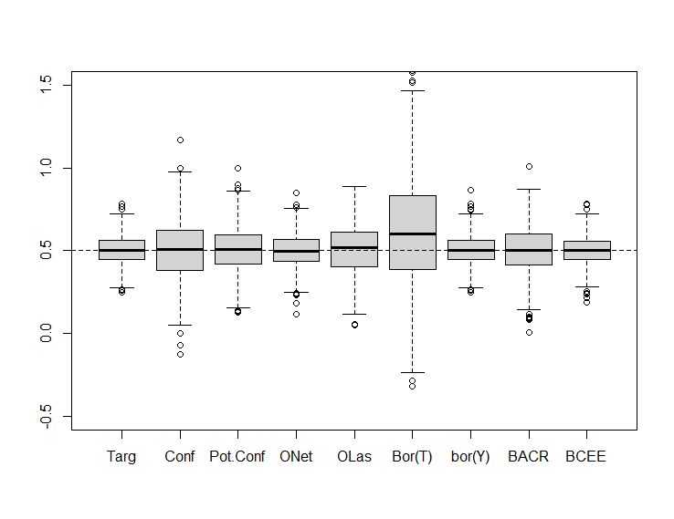
(a)

(b)

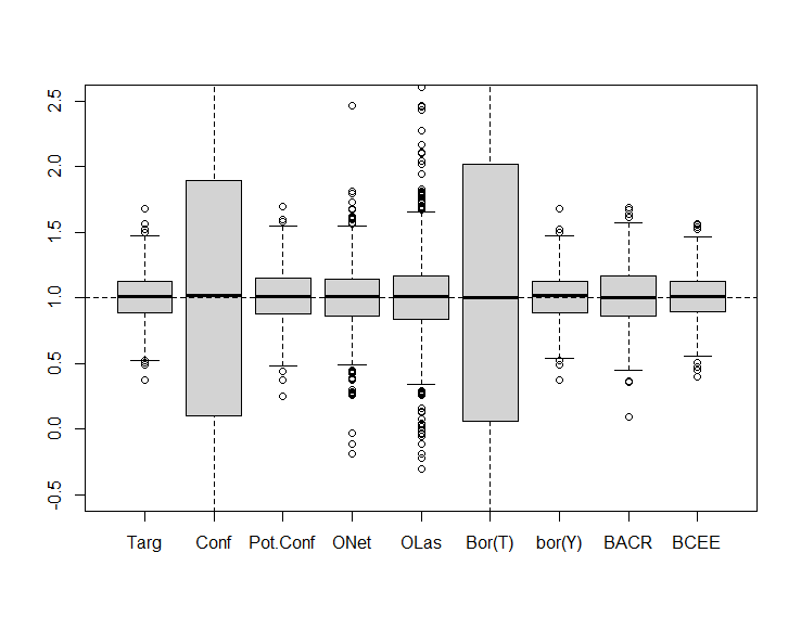
(c)

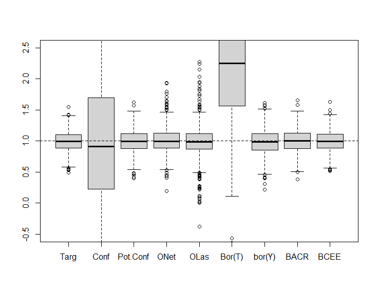
(d)

Figure 1: Average Treatment effect on the treated (ATT) for (a) Scenario 1A (b) Scenario 1B (c) Scenario 2A (d) Scenario 2B. Horizontal dashed line indicate the true treatment effect.

BAC, Bor(T), and Bor(Y) are omitted in the figure 1(b) due to the lack of matched pairs. Scenario 1B has 100 variables and high correlation ($\rho=0.5$). In such situations, BAC, Bor(T), and Bor(Y) select most of the variables including the spurious variables. It is almost impossible to find a sufficiently large matched set of sample from 1000 data points. However, the proposed outcome adaptive method along with outcome adaptive lasso and BCEE can identify confounders and the outcome predictors. In addition, recent literature [Brookhart et al., 2006, Shortreed & Ertefaie, 2017, Ertefaie et al., 2018a, b] suggest that considering only the treatment predictors does not reduce bias but inflate variance of the estimate. Our experiment also shows similar result as we can see in figure 1 (a), (c), and (d), Bor(T) which considers only the treatment predictors has the most variance in ATT among all the variable selection techniques.

In figure 2, we present the proportion of the time a variable is selected by the variable selection techniques for different scenarios. In scenario 1A and 1B, our target is to select the confounders (variables $X_{1},\cdots,X_{10}$) and the outcome predictors (variables $X_{11},\cdots,X_{20}$). In scenario 2A and 2B, an ideal variable selection algorithm should select variables $X_{1},\cdots,X_{4}$ among which, first two are confounders and the last two are outcome predictors. In almost all the cases, outcome adaptive elastic-net selects the confounders and in majority of the cases, it selects the outcome predictors. BCEE closely follows the target by selecting all the confounders and outcome predictors. However, it often selects some spurious variables in the process. Outcome adaptive lasso also performs well in selecting the confounders but it overly penalizes the outcome predictors. BAC, Bor(T), and Bor(Y) performs poorly in this metric and often selects spurious variables.

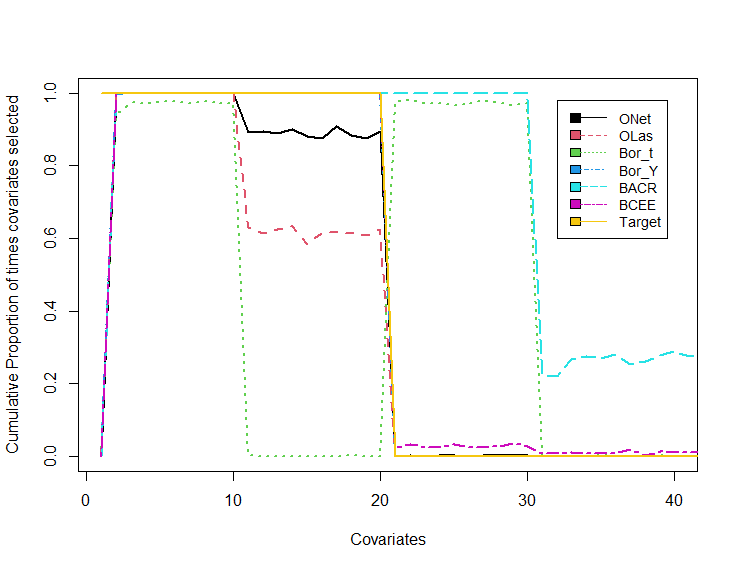
(a)

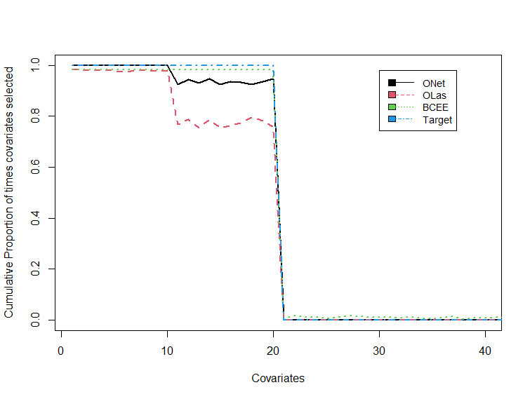
(b)

(c)

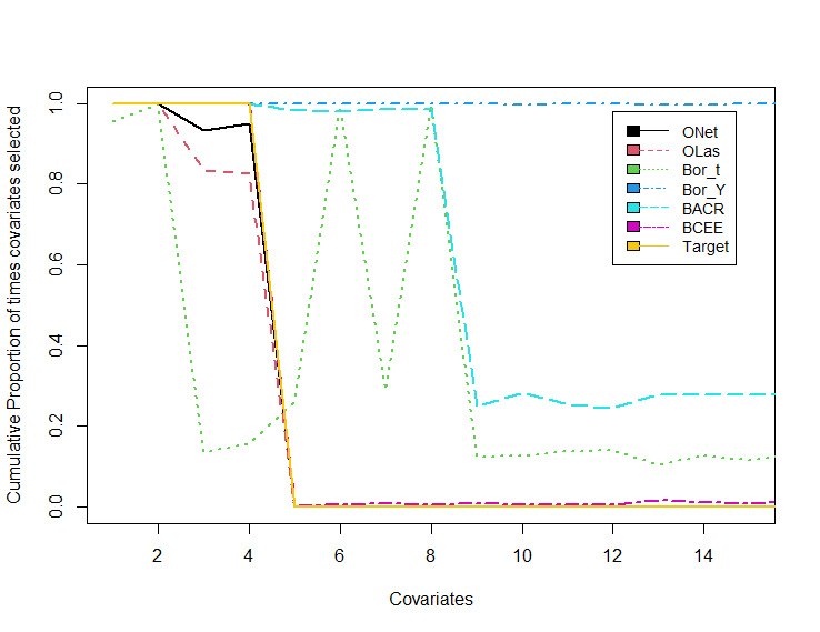
(d)

Figure 2: Proportion of the time variables selected in (a) Scenario 1A (b) Scenario 1B (c) Scenario 2A (d) Scenario 2B.

5 Conclusion

In this paper, we discuss the variable selection problem in causal inference. Variable selection problem is extensively studies in machine learning literature, however, the objective of this problem in the context of causal inference is quite different. Here, we have to select variables that are associated with multiple factors. To that end, we propose an Outcome adaptive elastic-net method that uses a variable penalty function instead of constant penalty function of elastic-net. First, we estimate the strength of association of the variables to the outcome by ordinary least square regression. Then, we use the inverse of these estimates in the elastic-net regularization to create a variable penalty function. This variable regularization ensures that the outcome predictors are less penalized in the treatment model and selects all the confounders and outcome predictors. We evaluate the performance of the proposed techniques on bias, variance and proportion of the time right variables are selected. Our analysis shows that the proposed outcome adaptive technique performs superiorly compared to the state-of-the-art methods. In the future, we plan to perform analysis on the properties of outcome adaptive elastic-net such as the possibility of achieving the oracle properties. In addition, we plan to develop case studies with real-world high dimensional data to present the applicability of the proposed method and additional guidelines for the users.

References

- Abadie & Imbens [2006] Abadie, A., & Imbens, G. W. (2006). Large sample properties of matching estimators for average treatment effects. Econometrica, 74, 235–267. URL: https://onlinelibrary.wiley.com/doi/abs/10.1111/j.1468-0262.2006.00655.x. doi:10.1111/j.1468-0262.2006.00655.x.
- Austin et al. [2013] Austin, P. C., Tu, J. V., Ho, J. E., Levy, D., & Lee, D. S. (2013). Using methods from the data-mining and machine-learning literature for disease classification and prediction: a case study examining classification of heart failure subtypes. Journal of clinical epidemiology, 66, 398–407.
- Brookhart et al. [2006] Brookhart, M. A., Schneeweiss, S., Rothman, K. J., Glynn, R. J., Avorn, J., & Stürmer, T. (2006). Variable selection for propensity score models. American journal of epidemiology, 163, 1149–1156.
- Ertefaie et al. [2018a] Ertefaie, A., Asgharian, M., & Stephens, D. A. (2018a). Variable selection in causal inference using a simultaneous penalization method. Journal of Causal Inference, 6.
- Ertefaie et al. [2018b] Ertefaie, A., Asgharian, M., & Stephens, D. A. (2018b). Variable selection in causal inference using a simultaneous penalization method. Journal of Causal Inference, 6.
- Holland [1986] Holland, P. W. (1986). Statistics and causal inference. Journal of the American Statistical Association, 81, 945–960.
- Iacus et al. [2011] Iacus, S. M., King, G., & Porro, G. (2011). Multivariate matching methods that are monotonic imbalance bounding. Journal of the American Statistical Association, 106, 345–361. doi:10.1198/jasa.2011.tm09599.
- [8] Judea, P. (). The foundations of causal inference. Sociological Methodology, 40, 75–149. doi:10.1111/j.1467-9531.2010.01228.x.
- King & Nielsen [2019] King, G., & Nielsen, R. (2019). Why propensity scores should not be used for matching. Political Analysis, 27.
- Kursa et al. [2020] Kursa, M. B., Rudnicki, W. R., & Kursa, M. M. B. (2020). Package ‘boruta’.
- Lee et al. [2010] Lee, B. K., Lessler, J., & Stuart, E. A. (2010). Improving propensity score weighting using machine learning. Statistics in medicine, 29, 337–346.
- Lin et al. [2015] Lin, W., Feng, R., & Li, H. (2015). Regularization methods for high-dimensional instrumental variables regression with an application to genetical genomics. Journal of the American Statistical Association, 110, 270–288.
- Nikolaev et al. [2013] Nikolaev, A. G., Jacobson, S. H., Cho, W. K. T., Sauppe, J. J., & Sewell, E. C. (2013). Balance optimization subset selection (boss): An alternative approach for causal inference with observational data. Operations Research, 61, 398–412. doi:10.1287/opre.1120.1118.
- Pearl [2009] Pearl, J. (2009). Causality. Cambridge university press.
- Pearl [2012] Pearl, J. (2012). On a class of bias-amplifying variables that endanger effect estimates. arXiv preprint arXiv:1203.3503, .
- Rosenbaum [2017] Rosenbaum, P. R. (2017). Imposing minimax and quantile constraints on optimal matching in observational studies. Journal of Computational and Graphical Statistics, 26, 66–78. doi:10.1080/10618600.2016.1152971.
- Rosenbaum & Rubin [1983] Rosenbaum, P. R., & Rubin, D. B. (1983). The central role of the propensity score in observational studies for causal effects. Biometrika, 70, 41–55. doi:10.1093/biomet/70.1.41.
- Rosenbaum & Rubin [1985] Rosenbaum, P. R., & Rubin, D. B. (1985). Constructing a control group using multivariate matched sampling methods that incorporate the propensity score. The American Statistician, 39, 33–38.
- Rosenbaum et al. [2010] Rosenbaum, P. R. et al. (2010). Design of observational studies volume 10. Springer.
- Rotnitzky et al. [2010] Rotnitzky, A., Li, L., & Li, X. (2010). A note on overadjustment in inverse probability weighted estimation. Biometrika, 97, 997–1001.
- Rubin [1973] Rubin, D. (1973). The use of matched sampling and regression adjustment to remove bias in observational studies. Biometrics, 29. doi:10.2307/2529685.
- Rubin [1979] Rubin, D. B. (1979). Using multivariate matched sampling and regression adjustment to control bias in observational studies. Journal of the American Statistical Association, 74, 318–328.
- Schnitzer et al. [2016] Schnitzer, M. E., Lok, J. J., & Gruber, S. (2016). Variable selection for confounder control, flexible modeling and collaborative targeted minimum loss-based estimation in causal inference. The international journal of biostatistics, 12, 97–115.
- Shortreed & Ertefaie [2017] Shortreed, S. M., & Ertefaie, A. (2017). Outcome-adaptive lasso: Variable selection for causal inference. Biometrics, 73, 1111–1122.
- [25] Singh, S. J., & D., G. R. (). A matching method for improving covariate balance in cost-effectiveness analyses. Health Economics, 21, 695–714. doi:10.1002/hec.1748.
- Stuart [2010] Stuart, E. A. (2010). Matching methods for causal inference: A review and a look forward. Statist. Sci., 25, 1–21. doi:10.1214/09-STS313.
- Talbot & Beaudoin [2020] Talbot, D., & Beaudoin, C. (2020). A generalized double robust bayesian model averaging approach to causal effect estimation with application to the study of osteoporotic fractures. arXiv preprint arXiv:2003.11588, .
- Talbot et al. [2015a] Talbot, D., Lefebvre, G., & Atherton, J. (2015a). The bayesian causal effect estimation algorithm. Journal of Causal Inference, 3, 207–236.
- Talbot et al. [2015b] Talbot, D., Lefebvre, G., Atherton, J., Chiu, Y., Talbot, M. D., Rcpp, I., Rcpp, L., & RcppArmadillo Depends, B. (2015b). Package ‘bcee’.
- VanderWeele & Shpitser [2011] VanderWeele, T. J., & Shpitser, I. (2011). A new criterion for confounder selection. Biometrics, 67, 1406–1413.
- Vansteelandt [2012] Vansteelandt, S. (2012). Bayesian effect estimation accounting for adjustment uncertainty discussions. Biometrics, 68, 665–678.
- Wang [2016] Wang, C. (2016). Package ‘bacr’.
- Wang et al. [2012] Wang, C., Parmigiani, G., & Dominici, F. (2012). Bayesian effect estimation accounting for adjustment uncertainty. Biometrics, 68, 661–671.
- Wang et al. [2021] Wang, T., Morucci, M., Awan, M. U., Liu, Y., Roy, S., Rudin, C., & Volfovsky, A. (2021). Flame: A fast large-scale almost matching exactly approach to causal inference. Journal of Machine Learning Research, 22, 1–41.
- Westreich et al. [2010] Westreich, D., Lessler, J., & Funk, M. J. (2010). Propensity score estimation: neural networks, support vector machines, decision trees (cart), and meta-classifiers as alternatives to logistic regression. Journal of clinical epidemiology, 63, 826–833.
- Wilson & Reich [2014] Wilson, A., & Reich, B. J. (2014). Confounder selection via penalized credible regions. Biometrics, 70, 852–861.
- Wooldridge [2016] Wooldridge, J. M. (2016). Should instrumental variables be used as matching variables? Research in Economics, 70, 232–237.
- Zou [2006] Zou, H. (2006). The adaptive lasso and its oracle properties. Journal of the American statistical association, 101, 1418–1429.
- Zou & Hastie [2005] Zou, H., & Hastie, T. (2005). Regularization and variable selection via the elastic net. Journal of the royal statistical society: series B (statistical methodology), 67, 301–320.
- Zou & Zhang [2009] Zou, H., & Zhang, H. H. (2009). On the adaptive elastic-net with a diverging number of parameters. Annals of statistics, 37, 1733.
- Zubizarreta [2012] Zubizarreta, J. R. (2012). Using mixed integer programming for matching in an observational study of kidney failure after surgery. Journal of the American Statistical Association, 107, 1360–1371. doi:10.1080/01621459.2012.703874.
- Zubizarreta [2015] Zubizarreta, J. R. (2015). Stable weights that balance covariates for estimation with incomplete outcome data. Journal of the American Statistical Association, 110, 910–922. doi:10.1080/01621459.2015.1023805.