Addressing Strong Correlation by Approximate Coupled-Pair Methods with Active-Space and Full Treatments of Three-Body Clusters

Abstract

When the number of strongly correlated electrons becomes larger, the single-reference coupled-cluster (CC) CCSD, CCSDT, etc. hierarchy displays an erratic behavior, while traditional multi-reference approaches may no longer be applicable due to enormous dimensionalities of the underlying model spaces. These difficulties can be alleviated by the approximate coupled-pair (ACP) theories, in which selected $(T_{2})^{2}$ diagrams in the CCSD amplitude equations are removed, but there is no generally accepted and robust way of incorporating connected triply excited ($T_{3}$) clusters within the ACP framework. It is also not clear if the specific combinations of $(T_{2})^{2}$ diagrams that work well for strongly correlated minimum-basis-set model systems are optimum when larger basis sets are employed. This study explores these topics by considering a few novel ACP schemes with the active-space and full treatments of $T_{3}$ correlations and schemes that scale selected $(T_{2})^{2}$ diagrams by factors depending on the numbers of occupied and unoccupied orbitals. The performance of the proposed ACP approaches is illustrated by examining the symmetric dissociations of the $\text{H}_{6}$ and $\text{H}_{10}$ rings using basis sets of the triple- and double-$\zeta$ quality and the $\text{H}_{50}$ linear chain treated with a minimum basis, for which the conventional CCSD and CCSDT methods fail.

I Introduction

The size extensive methods based on the exponential wave function ansatz Hubbard (1957); Hugenholtz (1957) of coupled-cluster (CC) theory Coester (1958); Coester and Kümmel (1960); Čížek (1966a, 1969); Čížek and Paldus (1971); Paldus et al. (1972),

$$|\Psi\rangle=\exp(T)|\Phi\rangle,$$ (1)

where

$$T=\sum_{n=1}^{N}T_{n}$$ (2)

is the cluster operator, $T_{n}$ is the $n$-particle–$n$-hole component of $T$, $N$ is the number of correlated electrons, and $|\Phi\rangle$ is the reference (e.g., Hartree–Fock) determinant defining the Fermi vacuum, have become a de facto standard for high-accuracy quantum chemistry calculations Paldus and Li (1999); Bartlett and Musiał (2007). This is, in significant part, related to the fact that the conventional single-reference CC hierarchy, including the CC approach with singles and doubles (CCSD), where $T$ is truncated at $T_{2}$ Purvis and Bartlett (1982); Cullen and Zerner (1982); Scuseria et al. (1987); Piecuch and Paldus (1989), the CC method with singles, doubles, and triples (CCSDT), where $T$ is truncated at $T_{3}$ Noga and Bartlett (1987); Scuseria and Schaefer (1988); Watts and Bartlett (1990), the CC approach with singles, doubles, triples, and quadruples (CCSDTQ), where $T$ is truncated at $T_{4}$ Oliphant and Adamowicz (1991a); Kucharski and Bartlett (1991, 1992); Piecuch and Adamowicz (1994a), etc., and its extensions to excited states and properties other than energy through the equation-of-motion Emrich (1981); Geertsen et al. (1989); Stanton and Bartlett (1993); Kowalski and Piecuch (2001a, b); Kucharski et al. (2001); Kállay and Gauss (2004); Hirata (2004) and linear response Monkhorst (1977); Dalgaard and Monkhorst (1983); Mukherjee and Mukherjee (1979); Sekino and Bartlett (1984); Takahashi and Paldus (1986); Koch and Jørgensen (1990); Koch et al. (1990); Kondo et al. (1995, 1996) formalisms rapidly converge to the exact, full configuration interaction (FCI), limit in weakly correlated systems. Higher-order CC methods, such as CCSDT and CCSDTQ, can also describe multi-reference situations involving smaller numbers of strongly correlated electrons, encountered, for example, when single and double bond dissociations are examined, allowing one to capture the relevant many-electron correlation effects in a conceptually straightforward fashion through particle–hole (p–h) excitations from a single determinant.

Unfortunately, the conventional CCSD, CCSDT, CCSDTQ, etc.  hierarchy may exhibit an erratic behavior and the lack of systematic convergence toward the exact, FCI, limit, if the system under consideration is characterized by the strong entanglement of larger numbers of electrons, as in the Mott metal–insulator transitions Mott (1949, 1968, 1990), which can be modeled by the Hubbard Hamiltonian Hubbard (1963, 1964a, 1964b) (see, e.g., Refs. Vollhardt (1984); Imada et al. (1998) and references therein) or the linear chains, rings, or cubic lattices of the equally spaced hydrogen atoms that change from a weakly correlated metallic state at compressed geometries to an insulating state with strong correlations in the dissociation region (see, e.g., Refs. Hachmann et al. (2006); Bendazzoli et al. (2011); Motta et al. (2017); Tsuchimochi and Scuseria (2009); Sinitskiy et al. (2010); Kats and Manby (2013); Pastorczak et al. (2017); Stair and Evangelista (2020)). The analogous challenges apply to the strongly correlated $\pi$-electron networks in cyclic polyenes Pauncz et al. (1962a, b), as described by the Hubbard and Pariser–Parr–Pople (PPP) Pariser and Parr (1953a, b); Pople (1953) Hamiltonians, which can be used to model one-dimensional metallic-like systems with Born–von Kármán periodic boundary conditions and a half-filled band Paldus et al. (1984a, b); Takahashi and Paldus (1985); Piecuch et al. (1990); Piecuch and Paldus (1991); Paldus and Piecuch (1992); Piecuch et al. (1992); Podeszwa et al. (2002). When the numbers of strongly correlated electrons and open-shell sites from which these electrons originate become larger, traditional multi-reference methods of the CC Paldus and Li (1999); Bartlett and Musiał (2007); Lindgren and Mukherjee (1987); Piecuch and Kowalski (2002); Lyakh et al. (2012); Evangelista (2018) and non-CC Szalay et al. (2012); Roca-Sanjuán et al. (2012); Chattopadhyay et al. (2016) types, which typically build upon complete active-space self-consistent field (CASSCF) Ruedenberg et al. (1982); Roos (1987), become inapplicable as well (in part, due to rapidly growing dimensionalities of the underlying multi-configurational reference or model spaces with the numbers of active electrons and orbitals, which are further complicated by considerable additional computational costs of determining the remaining dynamical correlation effects needed to obtain a quantitative description). Even the increasingly popular and undoubtedly promising substitutes for CASSCF, such as the density-matrix renormalization group (DMRG) approach White (1992); White and Martin (1999); Mitrushenkov et al. (2001); Chan and Head-Gordon (2002); Chan and Sharma (2011); Keller et al. (2015); Chan et al. (2016) (cf. Ref. Baiardi and Reiher (2020) for a recent perspective), FCI Quantum Monte Carlo Booth et al. (2009); Cleland et al. (2010); Dobrautz et al. (2019); Ghanem et al. (2019, 2020), and various selected CI techniques Whitten and Hackmeyer (1969); Bender and Davidson (1969); Huron et al. (1973); Buenker and Peyerimhoff (1974); Schriber and Evangelista (2016, 2017); Tubman et al. (2016, 2020); Liu and Hoffmann (2016); Zhang et al. (2020); Holmes et al. (2016); Sharma et al. (2017); Li et al. (2018); Garniron et al. (2017, 2019), or methods that replace complete active spaces by their incomplete or multi-layer counterparts (cf., e.g., Refs. Malmqvist et al. (1990); Ivanic (2003a, b); Ma et al. (2011); Vogiatzis et al. (2015); Hermes and Gagliardi (2019) for selected examples), which allow one to use significantly larger numbers of active electrons and orbitals compared to CASSCF-based schemes, begin to wear out when the number of strongly correlated electrons is on the order of 40–50. This is especially true when one wants to capture the missing dynamical correlations (cf., e.g., Refs. Kurashige and Yanai (2011); Guo et al. (2016); Nakatani and Guo (2017); Sharma and Chan (2014); Freitag et al. (2017); Ma et al. (2016)) and use basis sets much larger than the minimum one. While there has been a lot of activity directed toward addressing these and related issues, the challenge of strong correlation remains, awaiting a satisfactory solution. It is, therefore, desirable to explore various unconventional methodologies capable of accurately describing weak as well as strong correlation regimes, especially those that formally belong to the single-reference CC framework, which is characterized by an ease of implementation and application that cannot be matched by genuine multi-reference theories. To do this, one has to understand the origin of the erratic behavior of conventional single-reference CC approaches in the presence of strong correlations.

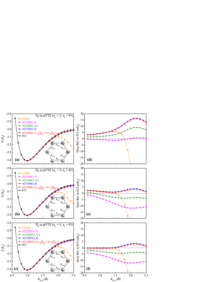
Figure 2: Ground-state PECs [panels (a)–(c)] and errors relative to FCI [panels (d)–(f)] for the symmetric dissociation of the $\text{H}_{6}$ ring resulting from the CCSD and various ACCSD [panels (a) and (d)], CCSDt and various ACCSDt [panels (b) and (e)], and CCSDT and various ACCSDT [panels (c) and (f)] calculations using the cc-pVTZ basis set. The CCSDt and ACCSDt approaches employed a minimum active space consisting of three occupied and three lowest-energy unoccupied MOs that correlate with the 1$s$ shells of the individual hydrogen atoms. The FCI PEC included in panels (a)–(c) is shown to facilitate comparisons.

The catastrophic failures of the traditional CCSD, CCSDT, CCSDTQ, etc. hierarchy in all of the aforementioned and similar situations, relevant to condensed matter physics, materials science, and the most severe cases of multiple bond breaking (e.g., the celebrated chromium dimer), are related to the observation that in order to describe wave functions for $N$ strongly correlated electrons one is essentially forced to deal with a FCI-level description of these $N$ electrons, which in a conventional CC formulation requires the incorporation of virtually all cluster components $T_{n}$, including $T_{N}$. Indeed, as shown, for example, in Fig. 2 of Ref. Degroote et al. (2016), using the 12-site, half-filled attractive pairing Hamiltonian with equally spaced levels, or slide 17 of Ref. Scuseria , in which the 10-site Hubbard Hamiltonian with half-filled band is examined, the higher-order $T_{n}$ components of the cluster operator, which normally decrease with $n$, remain large for larger $n$ values approaching $N$ in a strongly correlated regime. This is not a problem for the single-reference CC ansatz when the number of strongly correlated electrons $N$ is small (e.g., 2 in single bond breaking or 4 in double bond breaking), but becomes a major issue when $N$ is larger.

The consequences of the above observations manifest themselves in various, sometimes dramatic, ways. For example, one experiences a disastrous behavior of the traditional CCSD, CCSDT, CCSDTQ, etc. hierarchy, which produces large errors, branch point singularities, and unphysical complex solutions in calculations for strongly correlated one-dimensional systems modeled by the Hubbard and PPP Hamiltonians or $\text{H}_{n}$ rings, linear chains, and cubic lattices undergoing metal–insulator transitions Paldus et al. (1984a, b); Takahashi and Paldus (1985); Piecuch et al. (1990); Piecuch and Paldus (1991); Paldus and Piecuch (1992); Piecuch et al. (1992); Podeszwa et al. (2002); Degroote et al. (2016); Bulik et al. (2015); Gomez et al. (2017a, b); Stair and Evangelista (2020). One can also show, using spin-symmetry breaking and restoration arguments, combined with the Thouless theorem Thouless (1960, 1961) and a subsequent cluster analysis Čížek et al. (1969) of projected unrestricted Hartree–Fock (PUHF) wave functions similar to Refs. Paldus et al. (1984c); Piecuch et al. (1996a), that if we insist on the wave function ansatz in terms of the $T_{2}$ cluster component, the resulting strongly correlated PUHF state has a non-intuitive polynomial rather than the usual exponential form Qiu et al. (2016, 2017); Henderson and Scuseria (2017) (cf., also, Refs. Degroote et al. (2016); Gomez et al. (2017a, b)). This means that in seeking a computationally manageable CC-type solution to a problem of strong correlation involving the entanglement of many electrons, which would avoid the combinatorial scaling of FCI while eliminating failures of the CCSD, CCSDT, CCSDTQ, etc. hierarchy, one has to resign from the conventional CC treatments in which the cluster operator $T$ is truncated at a given many-body rank and all terms resulting from the exponential wave function ansatz are retained.

Among the most interesting solutions in this category are the approaches discussed in Refs. Degroote et al. (2016); Bulik et al. (2015); Gomez et al. (2017a, b); Qiu et al. (2016, 2017); Henderson and Scuseria (2017); Limacher et al. (2013); Henderson et al. (2014a, b); Stein et al. (2014); Shepherd et al. (2014, 2016); Gomez et al. (2016); Boguslawski and Tecmer (2017); Johnson et al. (2017); Marie et al. (2021). Another promising direction, which is the focus of this study, is the idea of the approximate coupled-pair (ACP) approaches Paldus et al. (1984a, b); Takahashi and Paldus (1985); Piecuch et al. (1990); Piecuch and Paldus (1991); Paldus and Piecuch (1992); Piecuch et al. (1992); Podeszwa et al. (2002); Piecuch et al. (1996a); Paldus et al. (1984c); Piecuch and Paldus (1990); Adams et al. (1981a); Jankowski and Paldus (1980); Adams et al. (1981b); Chiles and Dykstra (1981a); Bachrach et al. (1981); Piecuch et al. (1995) and their various more recent reincarnations or modifications, including the 2CC approach and its $n$CC extensions Bartlett and Musiał (2006); Musiał and Bartlett (2007), the orbital invariant coupled electron pair approximation with an extensive renormalized triples correction Nooijen and Le Roy (2006), the parameterized CCSD methods Huntington and Nooijen (2010) and their CCSDT-type counterparts Rishi and Valeev (2019), and the distinguishable cluster approximation with doubles (DCD) or singles and doubles (DCSD) Kats and Manby (2013); Kats (2014); Kats et al. (2015); Kats (2016, 2018) (see, also, Refs. Rishi et al. (2016, 2017, 2019)) and its DCSD(T) Kats (2016) and DCSDT Kats and Köhn (2019); Schraivogel and Kats (2021); Rishi and Valeev (2019) extensions to connected triples (see Ref. Paldus (2017) for a review). At the doubles or singles and doubles levels, the ACP methods have the relatively inexpensive $n_{\text{o}}^{2}n_{\text{u}}^{4}$ or ${\mathscr{N}}^{6}$ computational costs similar to CCD/CCSD, but by using the appropriately chosen subsets of non-linear $(T_{2})^{2}$ diagrams of the CCD/CCSD amplitude equations, they greatly improve the performance of CCD/CCSD in strongly correlated situations, including single and multiple bond dissociations Kats and Manby (2013); Huntington and Nooijen (2010); Kats (2014); Kats et al. (2015); Kats (2016, 2018); Rishi et al. (2016); Piecuch et al. (1996b) and, what is particularly intriguing, the low-dimensional metallic-like systems and symmetrically stretched hydrogen rings, linear chains, and cubic lattices, where the conventional CC treatments completely break down Kats and Manby (2013); Paldus et al. (1984a, b); Takahashi and Paldus (1985); Piecuch et al. (1990); Piecuch and Paldus (1991); Paldus and Piecuch (1992); Piecuch et al. (1992); Podeszwa et al. (2002) (we use the usual notation in which $n_{\text{o}}$ and $n_{\text{u}}$ are the numbers of correlated occupied and unoccupied orbitals, respectively, and ${\mathscr{N}}$ is a measure of the system size). As further elaborated on in Section II, these improvements in the performance of conventional single-reference CC approaches are not a coincidence. One can prove that there exist subsets of CCSD diagrams that result in an exact description of certain strongly correlated minimum-basis-set model systems Piecuch and Paldus (1991); Piecuch et al. (1996a); Paldus et al. (1984c), i.e., the ACP methodologies provide a rigorous basis for developing relatively inexpensive CC-like schemes for strong correlations (a multi-reference extension of the ACP ideas can also help genuine multi-reference CC approaches, especially when multi-determinantal model spaces become inadequate Piecuch et al. (1993a), but in this study we focus on the single-reference ACP framework).

Having stated all of the above, there remain several open problems that need to be addressed before the ACP methods can be routinely applied to realistic strongly correlated systems, i.e., systems involving larger numbers of strongly correlated electrons described by ab initio Hamiltonians and larger basis sets. One of the main problems is the neglect of connected triply excited ($T_{3}$) clusters in typical ACP methods. The low-dimensional model systems with small band gaps, such as the aforementioned cyclic polyenes near their strongly correlated limits, do not suffer from this a lot Piecuch et al. (1990); Paldus and Piecuch (1992), since their accurate description relies on $T_{n}$ clusters with even values of $n>2$, but one cannot produce quantitative results in the majority of realistic chemistry applications without $T_{3}$. The previous attempts to incorporate connected triply excited clusters within the ACP framework using conventional arguments based on the many-body perturbation theory (MBPT), similar to those exploited in ${\rm CCD[ST]}\equiv{\rm CCD{+}ST(CCD)}$ Raghavachari (1985), ${\rm CCSD[T]}\equiv{\rm CCSD{+}T(CCSD)}$ Urban et al. (1985), CCSD(T) Raghavachari et al. (1989), or CCSDT-1 Lee and Bartlett (1984); Lee et al. (1984), have only been partly successful Piecuch et al. (1990); Paldus and Piecuch (1992); Piecuch et al. (1992, 1996a, 1995); Kats (2016). They improved the ACP results in the weakly and moderately correlated regions of the cyclic polyene models, but did not help in the strongly correlated regime Piecuch et al. (1990); Paldus and Piecuch (1992). The aforementioned proposals how to include connected triply excited clusters in the parameterized CCSD and DCSD methods Kats (2016); Kats and Köhn (2019); Schraivogel and Kats (2021); Rishi and Valeev (2019) and the $n$CC approaches with $n>2$, which incorporate $T_{3}$ as well Bartlett and Musiał (2006); Musiał and Bartlett (2007), while being helpful in some cases of bond breaking, have never been applied to strongly correlated systems involving the entanglement of larger numbers of electrons. Thus, it remains unclear how to produce a computationally efficient ACP-type procedure that would include the information about connected triply excited clusters and work well in such situations at the same time. Another open problem pertains to the fact that the specific combinations of $(T_{2})^{2}$ diagrams that result in the ACP methods that work well in the strongly correlated regime of the minimum-basis-set model systems, such as the $\pi$-electron networks of cyclic polyenes, as described by the Hubbard and PPP Hamiltonians Paldus et al. (1984a, b); Takahashi and Paldus (1985); Piecuch et al. (1990); Piecuch and Paldus (1991); Paldus and Piecuch (1992); Piecuch et al. (1992); Podeszwa et al. (2002); Piecuch et al. (1996a); Paldus et al. (1984c); Piecuch and Paldus (1990) (see Section II for further information), may not necessarily be optimum when larger basis sets are employed.

We examine both of these topics in the present study. We deal with the problem of the missing $T_{3}$ physics by adopting the active-space CC ideas Kowalski and Piecuch (2001a, b); Oliphant and Adamowicz (1991b, 1992); Piecuch et al. (1993b); Piecuch and Adamowicz (1994b, a, 1995); Alexandrov et al. (1995); Ghose et al. (1995, 1996); Piecuch et al. (1999a, b); Kowalski and Piecuch (2001c, 2000); Kowalski et al. (2005); Piecuch et al. (2006); Gour et al. (2005, 2006); Gour and Piecuch (2006); Piecuch (2010); Shen and Piecuch (2013, 2014); Ajala et al. (2017) to incorporate the dominant triply excited amplitudes in the ACP methods in a robust, yet computationally affordable, manner. We show that the active-space triples ACP approaches examined in this work, which, following the naming convention introduced in Refs. Piecuch et al. (1999a, b), are collectively abbreviated as ACCSDt, do not suffer from the previously observed Piecuch et al. (1990); Paldus and Piecuch (1992) convergence problems resulting from the use of MBPT-based estimates of $T_{3}$ contributions within the ACP framework in a strongly correlated regime. Furthermore, by incorporating the leading triply excited cluster amplitudes in an iterative manner, the ACCSDt methods developed in this study allow the $T_{1}$ and $T_{2}$ clusters and, in particular, the subsets of $(T_{2})^{2}$ contributions responsible for an accurate description of strong correlations, to relax in the presence of the dominant $T_{3}$ amplitudes. The active-space ACCSDt schemes are also characterized by the systematic convergence toward their ACCSDT parents, in which $T_{3}$ clusters are treated fully, when the numbers of active occupied and active unoccupied orbitals used in the ACCSDt calculations increase. The issue of adjusting the $(T_{2})^{2}$ diagram combinations in the ACP amplitude equations to the numbers of occupied and unoccupied orbitals used in the calculations is explored in this study by testing a novel form of the ACP theory, abbreviated as $\text{ACCSD}(1{,}3\times\tfrac{n_{\text{o}}}{n_{\text{o}}+n_{\text{u}}}+4\times\tfrac{n_{\text{u}}}{n_{\text{o}}+n_{\text{u}}})$, and its extensions accounting for $T_{3}$ correlations, abbreviated as $\text{ACCSDt}(1{,}3\times\tfrac{n_{\text{o}}}{n_{\text{o}}+n_{\text{u}}}+4\times\tfrac{n_{\text{u}}}{n_{\text{o}}+n_{\text{u}}})$ and $\text{ACCSDT}(1{,}3\times\tfrac{n_{\text{o}}}{n_{\text{o}}+n_{\text{u}}}+4\times\tfrac{n_{\text{u}}}{n_{\text{o}}+n_{\text{u}}})$, which utilize the $n_{\rm o}$- and $n_{\rm u}$-dependent scaling factors multiplying the $(T_{2})^{2}$ diagrams kept in the calculations. At the singles and doubles level and when $n_{\rm o}=n_{\rm u}$, i.e., when a minimum basis set is employed, the $\text{ACCSD}(1{,}3\times\tfrac{n_{\text{o}}}{n_{\text{o}}+n_{\text{u}}}+4\times\tfrac{n_{\text{u}}}{n_{\text{o}}+n_{\text{u}}})$ scheme reduces to the DCSD approach of Ref. Kats and Manby (2013), which, in analogy to the closely related ACP-D13 and ACP-D14 methods introduced in Ref. Piecuch and Paldus (1991), becomes exact in the strongly correlated limit of cyclic polyenes modeled by the Hubbard and PPP Hamiltonians. At the same time, the $\text{ACCSDT}(1{,}3\times\tfrac{n_{\text{o}}}{n_{\text{o}}+n_{\text{u}}}+4\times\tfrac{n_{\text{u}}}{n_{\text{o}}+n_{\text{u}}})$ approach becomes equivalent to the ACP-D14 method of Ref. Piecuch and Paldus (1991) augmented with $T_{1}$ and $T_{3}$ clusters when $n_{\rm o}\ll n_{\rm u}$, which does, based on our numerical tests, including those discussed in Section III, improve the $\text{ACCSDT}(1{,}\tfrac{3+4}{2})$ results, obtained by embedding $\text{ACCSD}(1{,}\tfrac{3+4}{2})$ = DCSD in CCSDT, in calculations using larger basis sets. By examining the symmetric dissociations of the $\text{H}_{6}$ and $\text{H}_{10}$ rings, as described by basis sets of the triple- and double-$\zeta$ quality, for which the exact, FCI, calculations are feasible, and the $\text{H}_{50}$ linear chain treated with a minimum basis, for which the nearly exact, DMRG, results are available Hachmann et al. (2006), we show that the active-space $\text{ACCSDt}(1{,}3\times\tfrac{n_{\text{o}}}{n_{\text{o}}+n_{\text{u}}}+4\times\tfrac{n_{\text{u}}}{n_{\text{o}}+n_{\text{u}}})$ method and its $\text{ACCSDT}(1{,}3\times\tfrac{n_{\text{o}}}{n_{\text{o}}+n_{\text{u}}}+4\times\tfrac{n_{\text{u}}}{n_{\text{o}}+n_{\text{u}}})$ parent accurately reproduce the FCI ($\text{H}_{6}$ and $\text{H}_{10}$) and DMRG ($\text{H}_{50}$) energetics, while improving the $\text{ACCSD}(1{,}3\times\tfrac{n_{\text{o}}}{n_{\text{o}}+n_{\text{u}}}+4\times\tfrac{n_{\text{u}}}{n_{\text{o}}+n_{\text{u}}})$ results and eliminating catastrophic failures of CCSD and CCSDT in the strongly correlated regions. Because of the use of basis sets larger than a minimum one in calculations for the $\text{H}_{6}$ and $\text{H}_{10}$ ring systems, we also demonstrate that $\text{ACCSDt}(1{,}3\times\tfrac{n_{\text{o}}}{n_{\text{o}}+n_{\text{u}}}+4\times\tfrac{n_{\text{u}}}{n_{\text{o}}+n_{\text{u}}})$ and other ACCSDt schemes recover the corresponding ACCSDT results, including a strongly correlated regime, at the tiny fraction of the computational cost.

II Theory and Computational Details

II.1 Overview of the ACP Schemes

Historically, a variety of different ways of rationalizing the ACP and related methods using subsets of non-linear diagrams within a CCD/CCSD framework have been considered (cf. Refs. Kats and Manby (2013); Paldus et al. (1984a); Piecuch and Paldus (1991); Paldus and Piecuch (1992); Piecuch et al. (1996a); Paldus et al. (1984c); Piecuch and Paldus (1990); Adams et al. (1981a); Jankowski and Paldus (1980); Adams et al. (1981b); Chiles and Dykstra (1981a); Bachrach et al. (1981); Bartlett and Musiał (2006); Musiał and Bartlett (2007); Nooijen and Le Roy (2006); Huntington and Nooijen (2010); Paldus (2017)). Given the objectives of this study, we begin our discussion with the past numerical observations and mathematical analyses that allow us to understand the ability of such methods to describe strongly correlated electrons. Let us focus for a moment on a simpler CCD case, so that we do not have to worry about the less essential, but more numerous, contributions containing the $T_{1}$ cluster component. Using the language of Goldstone–Brandow (Goldstone–Hugenholtz) diagrams, utilized in the derivations whenever the orthogonally spin-adapted description Piecuch et al. (1996a); Paldus et al. (1984c); Piecuch and Paldus (1990); Čížek (1966b); Paldus et al. (1977); Paldus (1977); Adams and Paldus (1979); Chiles and Dykstra (1981b); Takahashi and Paldus (1986); Piecuch and Paldus (1989); Geertsen et al. (1991); Piecuch and Paldus (1992, 1994), important for the understanding of the earliest ACP models, is desired, one may show that of the five Goldstone–Brandow $(T_{2})^{2}$ diagrams of the CCD amplitude equations,

$${}_{S_{r}}\!\matrixelement{\Phi_{IJ}^{AB}}{[H_{N}(1+T_{2}+\tfrac{1}{2}T_{2}^{2})]_{C}}{\Phi}={}_{S_{r}}\!\matrixelement{\Phi_{IJ}^{AB}}{[H_{N}(1+T_{2})]_{C}}{\Phi}+\sum_{k=1}^{5}\Lambda_{k}^{(2)}(AB,IJ;S_{r})=0,$$ (3)

represented in Eq. (3) by the $\Lambda_{k}^{(2)}(AB,IJ;S_{r}),k=\text{1--5},$ terms and shown in Fig. 1 as diagrams (1)–(5), only two, namely, diagrams (4) and (5), which are separable over the hole line(s), are needed to eliminate the pole singularities plaguing linearized CCD in situations involving electronic quasi-degeneracies Paldus et al. (1984a, b); Takahashi and Paldus (1985); Adams et al. (1981a); Jankowski and Paldus (1980); Adams et al. (1981b). Here, we use the notation in which $H_{N}=H-\langle\Phi|H|\Phi\rangle$ is the Hamiltonian in the normal-ordered form and subscript $C$ indicates the connected operator product. The $\ket{\Phi_{IJ}^{AB}}_{S_{r}}$ states in Eq. (3), where $I$ and $J$ designate the occupied and $A$ and $B$ the unoccupied spatial orbitals in the closed-shell reference determinant $|\Phi\rangle$ and $S_{r}=0$ or 1 is the intermediate spin quantum number, represent the singlet particle-particle–hole-hole (pp–hh) coupled orthogonally spin-adapted doubly excited configuration state functions (CSFs). Using these functions, the $T_{2}$ operator entering Eq. (3), represented in Fig. 1 by the oval-shaped vertices, is defined as

$$T_{2}|\Phi\rangle=\sum_{I\leq J,A\leq B}\sum_{S_{r}=0}^{1}t_{AB}^{IJ}(S_{r})\,\ket{\Phi_{IJ}^{AB}}_{S_{r}}=\frac{1}{4}\sum_{IJAB}\sum_{S_{r}=0}^{1}(N_{IJ}^{AB})^{-2}\,t_{AB}^{IJ}(S_{r})\,\ket{\Phi_{IJ}^{AB}}_{S_{r}},$$ (4)

where $t_{AB}^{IJ}(S_{r})$ are the corresponding spin-adapted doubly excited cluster amplitudes and

$$N_{IJ}^{AB}=[(1+\delta_{IJ})(1+\delta_{AB})]^{-1/2},$$ (5)

with $\delta_{IJ}$ and $\delta_{AB}$ designating Kronecker deltas, is the appropriate normalization factor Piecuch et al. (1996a); Paldus et al. (1984c); Piecuch and Paldus (1990); Paldus et al. (1977); Paldus (1977); Adams and Paldus (1979); Piecuch and Paldus (1989). The ACP approach obtained using only the 4th and 5th $(T_{2})^{2}$ contributions in Eq. (3), $\Lambda_{4}^{(2)}(AB,IJ;S_{r})$ and $\Lambda_{5}^{(2)}(AB,IJ;S_{r})$, respectively, has originally been called ACP-D45 Adams et al. (1981a); Jankowski and Paldus (1980); Adams et al. (1981b) or ACCD Chiles and Dykstra (1981a); Bachrach et al. (1981). As shown in Refs. Paldus et al. (1984a, b); Takahashi and Paldus (1985); Adams et al. (1981a); Jankowski and Paldus (1980); Adams et al. (1981a, b); Chiles and Dykstra (1981a); Bachrach et al. (1981), using the aforementioned cyclic polyene models, ${\rm C}_{N}{\rm H}_{N}$, in a $\pi$-electron approximation, described by the Hubbard and PPP Hamiltonians, where one places $N=4n+2$, $n=1,2,\ldots,$ carbon atoms on a ring, and several ab initio systems, including small hydrogen clusters, beryllium atom, and small molecules, the ACP-D45 method is as accurate as CCD in weakly correlated cases with no electronic quasi-degeneracies, while representing an excellent approximation in strongly correlated, highly degenerate situations, where the linearized CCD Paldus et al. (1984a, b); Takahashi and Paldus (1985); Adams et al. (1981a); Jankowski and Paldus (1980); Adams et al. (1981b) or even the full CCD Paldus et al. (1984a, b); Takahashi and Paldus (1985); Piecuch et al. (1990); Piecuch and Paldus (1991); Paldus and Piecuch (1992); Piecuch et al. (1992), CCD corrected for connected triples via perturbative approximations of the CCD[ST] or CCSD[T] and CCSDT-1 types Piecuch et al. (1990); Paldus and Piecuch (1992); Piecuch et al. (1992), CCSDT Podeszwa et al. (2002), and CCSDTQ Podeszwa et al. (2002) are plagued with singularities or divergent behavior. At the time of the initial discovery of the ACP-D45 or ACCD scheme, this remarkable behavior was partially explained by the mutual cancellation of the contributions arising from the first three diagrams in Fig. 1, observed numerically Paldus et al. (1984a); Adams et al. (1981a); Jankowski and Paldus (1980); Adams et al. (1981b) and advocated mathematically by considering the limit of non-interacting electron pairs Chiles and Dykstra (1981a). However, this could not explain why the ACP-D45 approach, using only two of the five $(T_{2})^{2}$ Goldstone–Brandow diagrams of CCD, works so well in the strongly correlated, $\beta=0$, limit of the cyclic polyene models, where CCD completely fails, producing branch point singularities and complex solutions for cyclic polyenes with 14 or more carbon sites as $\beta$ approaches 0 from the weakly correlated $\beta\ll 0$ region Paldus et al. (1984a, b); Takahashi and Paldus (1985); Piecuch et al. (1990); Piecuch and Paldus (1991); Paldus and Piecuch (1992); Piecuch et al. (1992) ($\beta$ is the parameter scaling the one-electron part of the Hubbard or PPP Hamiltonians; in the Hubbard Hamiltonian case, $\beta$ is equivalent to $-t/U$, where $t$ and $U$ are the parameters controlling the kinetic energy characterizing the hopping of electrons between nearest neighbors and on-site electron-electron repulsion, respectively). In fact, it was observed that ACP-D45 is exact in the strongly correlated, $\beta=0$, limit of the Hubbard model Paldus et al. (1984a, b); Takahashi and Paldus (1985); Piecuch et al. (1990); Piecuch and Paldus (1991); Paldus and Piecuch (1992); Piecuch et al. (1992), while being accurate for the PPP Hamiltonian and other $\beta$ values. Other selections of CCD or CCSD $(T_{2})^{2}$ diagrams were considered by several authors in recent years Kats and Manby (2013); Bartlett and Musiał (2006); Musiał and Bartlett (2007); Huntington and Nooijen (2010); Kats (2014); Kats et al. (2015); Kats (2016, 2018); Rishi et al. (2016, 2017, 2019), with some choices being similar or even identical to the original ACP approaches examined in Refs. Paldus et al. (1984a, b); Takahashi and Paldus (1985); Piecuch et al. (1990); Piecuch and Paldus (1991); Paldus and Piecuch (1992); Piecuch et al. (1992); Podeszwa et al. (2002); Piecuch et al. (1996a); Paldus et al. (1984c); Piecuch and Paldus (1990); Adams et al. (1981a); Jankowski and Paldus (1980); Adams et al. (1981b); Chiles and Dykstra (1981a); Bachrach et al. (1981); Piecuch et al. (1995), seeking diagram combinations that work better than CCD/CCSD in bond breaking situations, but none of these recent studies have provided rigorous mathematical arguments why the ACP methods, such as ACP-D45, can be exact or nearly exact in strongly correlated situations of the type of those created by the cyclic polyene models in the $\beta\approx 0$ region.

The major breakthrough in the understanding of the superb performance of the ACP-D45 approach in a strongly correlated regime came in 1984 Paldus et al. (1984c), followed by two other key articles published in 1991 Piecuch and Paldus (1991) and 1996 Piecuch et al. (1996a). By performing cluster analysis Čížek et al. (1969) of the PUHF wave function within the orthogonally spin-adapted framework, in which the PUHF state was assumed to be exact, and using the philosophy of the externally corrected CC methods Piecuch et al. (1996a); Paldus et al. (1984c); Paldus (2017); Paldus and Planelles (1994); Stolarczyk (1994); Peris et al. (1997, 1999); Li and Paldus (1997, 1998, 2006); Xu and Li (2015); Deustua et al. (2018); Aroeira et al. (2021); Lee et al. (2021); Magoulas et al. (2021), the authors of Refs. Paldus et al. (1984c); Piecuch et al. (1996a) demonstrated that the $T_{4}$ cluster component extracted from PUHF with the help of the Thouless theorem and read into the CCD system, Eq. (3), (Ref. Paldus et al. (1984c)) or its CCSD extension (Ref. Piecuch et al. (1996a)) as the ${}_{S_{r}}\!\matrixelement{\Phi_{IJ}^{AB}}{(H_{N}T_{4})_{C}}{\Phi}$ contribution cancels out the first three of the five diagrams in Fig. 1, while multiplying the fifth diagram in the equations projected on the singlet pp–hh coupled orthogonally spin-adapted doubly excited $\ket{\Phi_{IJ}^{AB}}_{S_{r}}$ CSFs with the intermediate spin $S_{r}=1$ by a factor of 9 (in principle, the analogous $T_{3}$-containing contributions should have been read into the CCD or CCSD systems too, but they were not, since $T_{3}$ extracted from the PUHF wave function, represented as a CC state relative to the restricted Hartree–Fock (RHF) reference determinant, vanishes Paldus et al. (1984c); Piecuch et al. (1996a)). The PUHF wave function provides exact energies and cluster amplitudes for the PPP and Hubbard Hamiltonian models of cyclic polyenes in the strongly correlated, $\beta=0$, limit, so the resulting $\text{ACP-D}45_{9}$ theory, abbreviated as ACPQ Paldus et al. (1984c) or $\text{ACCD}^{\prime}$ Piecuch et al. (1996a), using $\Lambda_{4}^{(2)}(AB,IJ;S_{r})+(2S_{r}+1)^{2}\Lambda_{5}^{(2)}(AB,IJ;S_{r})$ instead of $\sum_{k=1}^{5}\Lambda_{k}^{(2)}(AB,IJ;S_{r})$ to represent the $(T_{2})^{2}$ contributions within the CCD system, Eq. (3), is mathematically exact in this limit, in complete agreement with the numerical observations Paldus et al. (1984a, b); Takahashi and Paldus (1985); Piecuch et al. (1990); Piecuch and Paldus (1991); Paldus and Piecuch (1992); Piecuch et al. (1992); Podeszwa et al. (2002) (the $T_{1}$ contributions can be ignored here, since $T_{1}=0$ for the cyclic polyene models described by the PPP and Hubbard Hamiltonians). The aforementioned factor of 9, which is simply the square of the multiplicity associated with the intermediate spin value $S_{r}=1$, was a result of using the orthogonally spin-adapted formalism; without using this formalism and without the exploitation of the appropriate many-body and angular momentum diagrammatic techniques in Refs. Piecuch et al. (1996a); Paldus et al. (1984c), one would not be able to see the emergence of $(2S_{r}+1)^{2}$ at the $\Lambda_{5}^{(2)}(AB,IJ;S_{r})$ term corresponding to diagram (5) in a transparent manner. The original derivation in Ref. Paldus et al. (1984c) assumed that the PUHF wave function has no singlet-coupled singly excited CSFs relative to RHF, which is true for the PPP and Hubbard Hamiltonian models of cyclic polyenes due to symmetry, but not in general, so the $\text{ACP-D}45_{9}=\text{ACPQ}=\text{ACCD}^{\prime}$ scheme and its more complete CCSD-level extension, where the $T_{1}$ clusters are included as well, termed $\text{ACCSD}^{\prime}$ Piecuch et al. (1996a), were rederived in Ref. Piecuch et al. (1996a). Reference Piecuch et al. (1996a) also examined the $\text{CCSDQ}^{\prime}$ approach and its triples-corrected $\text{CCSDQ}^{\prime}+\text{T}(\text{CCSDQ}^{\prime})=\text{CCSDQ}^{\prime}[\text{T}]$ extension, where one does not make any assumptions regarding the accuracy of PUHF and extracts the $T_{4}$ cluster component from a PUHF wave function as is, showing additional improvements in some cases, but our focus here is on the philosophy represented by the ACP methods, such as $\text{ACCSD}^{\prime}$. If the above factor of 9 at the fifth diagram in Fig. 1 for the $S_{r}=1$ case is ignored (and for the cyclic polyene models, as described by the PPP and Hubbard Hamiltonians, $\Lambda_{5}^{(2)}(AB,IJ;S_{r})$ is generally small), the $\text{ACP-D}45_{9}=\text{ACPQ}=\text{ACCD}^{\prime}$ scheme, derived in Ref. Paldus et al. (1984c) and extended to a singles and doubles level in Ref. Piecuch et al. (1996a), reduces to the original ACP-D45 or ACCD approach of Refs. Adams et al. (1981a); Jankowski and Paldus (1980); Adams et al. (1981b); Chiles and Dykstra (1981a); Bachrach et al. (1981). In fact, in the strongly correlated, $\beta=0$, limit of cyclic polyenes described by the Hubbard Hamiltonian, the $\Lambda_{5}^{(2)}(AB,IJ;S_{r}=1)$ term vanishes Piecuch and Paldus (1991), so that the ACP-D45 approximation becomes exact in this case, as observed numerically Paldus et al. (1984a, b); Takahashi and Paldus (1985); Piecuch et al. (1990); Piecuch and Paldus (1991); Paldus and Piecuch (1992); Piecuch et al. (1992). When the above factor of 9 is included, as in the $\text{ACP-D}45_{9}=\text{ACPQ}=\text{ACCD}^{\prime}$ or $\text{ACCSD}^{\prime}$ approaches, one ends up with an exact description of the strongly correlated, $\beta=0$, limit of cyclic polyenes with $4n+2$ carbons on a ring and described by either the Hubbard or PPP Hamiltonians. This result is independent of $n$, i.e., it remains valid in the thermodynamic limit.

There are other selections of the $(T_{2})^{2}$ diagrams entering the CCD or CCSD amplitude equations that can also be exact in the strongly correlated regimes of model Hamiltonians. In Ref. Piecuch and Paldus (1991), the exactness of $\text{ACP-D}45_{9}=\text{ACPQ}=\text{ACCD}^{\prime}$ in the strongly correlated, $\beta=0,$ limit of the cyclic polyene models described by the Hubbard and PPP Hamiltonians was re-examined using back substitution of the exact $T_{2}$ amplitudes extracted from a PUHF wave function into the CCD and $\text{ACP-D}45_{9}$ systems. By doing so, it was proven that the exact $T_{2}$ amplitudes satisfy the latter system, but not the former one, showing that $\text{ACP-D}45_{9}$ is exact when $\beta=0$ and CCD is not (as already mentioned, CCD behaves erratically in the $\beta=0$ limit). Encouraged by the usefulness of such an analysis, the authors of Ref. Piecuch and Paldus (1991) searched for other combinations of the CCD $(T_{2})^{2}$ diagrams that produce exact results at $\beta=0,$ discovering several possibilities. One of them, using diagrams (1) and (4) in Fig. 1 and defining the ACP-D14 approach, is $\Lambda_{1}^{(2)}(AB,IJ;S_{r})+\Lambda_{4}^{(2)}(AB,IJ;S_{r})$. As shown in Ref. Piecuch and Paldus (1991) for the cyclic polyene models, which have several symmetries, including the p–h symmetry, $\Lambda_{3}^{(2)}(AB,IJ;S_{r})=\Lambda_{4}^{(2)}(AB,IJ;S_{r})$, i.e., diagrams (3) and (4) in Fig. 1 are equivalent in this case. Thus, one can also propose two other methods, ACP-D13 and ACP-D1(3+4)/2, which correspond to the following expressions for the $(T_{2})^{2}$ contributions within a CCD or CCSD framework: $\Lambda_{1}^{(2)}(AB,IJ;S_{r})+\Lambda_{3}^{(2)}(AB,IJ;S_{r})$ and $\Lambda_{1}^{(2)}(AB,IJ;S_{r})+[\Lambda_{3}^{(2)}(AB,IJ;S_{r})+\Lambda_{4}^{(2)}(AB,IJ;S_{r})]/2$, respectively. All three methods, ACP-D13, ACP-D14, and ACP-D1(3+4)/2, are exact in the strongly correlated, $\beta=0,$ limit of cyclic polyenes described by the Hubbard and PPP Hamiltonians, i.e., it is worth considering them all. The performance of the ACP-D14 approach in the calculations for cyclic polyenes in the entire range of $\beta$ values, from the weakly to the strongly correlated regimes and systems as large as $\text{C}_{22}\text{H}_{22}$, was examined in Ref. Piecuch and Paldus (1991), showing the excellent and non-singular behavior similar to the $\text{ACP-D}45_{9}=\text{ACPQ}=\text{ACCD}^{\prime}$ methods tested in Refs. Paldus et al. (1984a, b); Takahashi and Paldus (1985); Piecuch et al. (1990); Piecuch and Paldus (1991); Paldus and Piecuch (1992); Piecuch et al. (1992). The calculations using the other two approaches, ACP-D13 and ACP-D1(3+4)/2, were not reported in Ref. Piecuch and Paldus (1991), since they would produce identical results due to the p–h symmetry intrinsic to the cyclic polyene models. The ACP-D1(3+4)/2 approach, rationalized by the 1991 analysis in Ref. Piecuch and Paldus (1991), is equivalent to the recently pursued DCD method of Refs. Kats and Manby (2013); Kats (2014); Kats et al. (2015); Kats (2016, 2018). By averaging diagrams (3) and (4), which are the p–h versions of each other, the ACP-D1(3+4)/2 = DCD model attempts to reinforce the p–h symmetry, even if there is none in the Hamiltonian. Time will tell if it is beneficial to do this in ab initio applications involving strongly correlated situations, that is, if using DCD and its CCSD-like extension, termed DCSD Kats and Manby (2013); Kats (2014); Kats et al. (2015); Kats (2016, 2018), is an overall better idea than using the older $\text{ACP-D}45_{9}=\text{ACPQ}=\text{ACCD}^{\prime}$ and $\text{ACCSD}^{\prime}$ approaches. The performance of the latter approach in bond breaking situations was examined as early as in 1996 Piecuch et al. (1996b), but our knowledge of the relative performance of these different ACP variants, especially in large-scale ab initio studies, is still rather limited, although various combinations of $(T_{2})^{2}$ diagrams within CCSD have been examined in Refs. Kats and Manby (2013); Huntington and Nooijen (2010); Kats (2014); Kats et al. (2015); Kats (2016, 2018); Rishi et al. (2016, 2019), showing encouraging results.

There is no doubt that numerical tests of the various ACP-type approximations will continue to be helpful, but in order for these methods to become successful and widely used in the longer term, especially in the examination of problems involving larger numbers of strongly correlated electrons that cannot be handled by the existing multi-reference methods, selected CI, or DMRG, one has to address several issues. The above discussion implies that the ACP-D13, ACP-D14, ACP-D1(3+4)/2 = DCD, and $\text{ACP-D}45_{9}=\text{ACPQ}=\text{ACCD}^{\prime}$ approaches, obtained by considering subsets of $(T_{2})^{2}$ diagrams within the CCD system, Eq. (3), and their extensions incorporating $T_{1}$ clusters are more robust than the traditional CCSD, CCSDT, CCSDTQ, etc. hierarchy in strongly correlated situations, but the main rationale behind their usefulness is based on considering strongly correlated limits of highly symmetric, minimum-basis-set, model Hamiltonians. It is not immediately obvious that the same combinations of $(T_{2})^{2}$ diagrams remain optimum when larger basis sets, required by quantitative ab initio quantum chemistry, are employed. More importantly, as already explained above, the $T_{3}$ physics is absent in the ACP approaches derived within a CCD/CCSD framework or its PUHF-driven externally corrected extensions, in which, as shown, for example, in Refs. Paldus et al. (1984c); Piecuch et al. (1996a), $T_{3}=0$. In other words, the ACP methods obtained by selecting and modifying $(T_{2})^{2}$ diagrams within CCD or CCSD, while capturing strong non-dynamical correlations in a computationally manageable fashion, even when the numbers of strongly correlated electrons are larger, and providing $T_{1}$ and $T_{2}$ clusters that are more accurate than those obtained with CCD or CCSD, offer incomplete information about dynamical correlation effects, which cannot be accurately described without the connected $T_{3}$ clusters. As pointed out in the Introduction, the previously developed ACP schemes corrected for the effects of connected triply excited clusters using arguments originating from MBPT Piecuch and Paldus (1990); Piecuch et al. (1996a, 1995) have only had partial success when examining cyclic polyene models Piecuch et al. (1990); Paldus and Piecuch (1992); Piecuch et al. (1992), whereas the recent attempts to include $T_{3}$ correlations in parameterized CCSD and DCSD Kats (2016); Kats and Köhn (2019); Schraivogel and Kats (2021); Rishi and Valeev (2019) or via the $n$CC hierarchy Bartlett and Musiał (2006); Musiał and Bartlett (2007) have not been applied to strongly correlated systems involving the entanglement of larger numbers of electrons that interest us in this study most. It is, therefore, useful to consider alternative ways of handling connected triply excited clusters within the ACP methodology that might result in practical computational schemes, while having the potential for working well in a strongly correlated regime. We discuss such approaches in the next subsection.

II.2 The Proposed ACP Approaches

In searching for the combinations of $(T_{2})^{2}$ diagrams that might potentially improve the ACP results corrected for $T_{3}$ correlations when larger basis sets are employed, it is worth noticing that one could retain the exactness of the ACP approaches using diagrams (1), (3), and (4) in Fig. 1 in the strongly correlated limit of cyclic polyenes, as described by the Hubbard and PPP Hamiltonians, by considering other combinations of diagrams (3) and (4) than those used in the ACP-D13, ACP-D14, and ACP-D1(3+4)/2 = DCD methods. One could, in fact, replace the $\sum_{k=1}^{5}\Lambda_{k}^{(2)}(AB,IJ;S_{r})$ contribution to the CCD system, Eq. (3), originating from the five $(T_{2})^{2}$ diagrams shown in Fig. 1, by

$$\Lambda_{1}^{(2)}(AB,IJ;S_{r})+\lambda\,\Lambda_{3}^{(2)}(AB,IJ;S_{r})+(1-\lambda)\,\Lambda_{4}^{(2)}(AB,IJ;S_{r})$$ (6)

with an arbitrary value of $\lambda$, and still be exact in the $\beta=0$ limit of the cyclic polyene models. In ACP-D1(3+4)/2 = DCD and its DCSD extension incorporating $T_{1}$ clusters, one uses $\lambda=\tfrac{1}{2},$ which is appropriate for cyclic polyenes, as described by the Hubbard and PPP Hamiltonians that have the p–h symmetry, and justified in the case of other strongly correlated systems, such as the hydrogen clusters examined in this work described by the ab initio Hamiltonians, as long as one uses a minimum basis set, for which the p–h symmetry is approximately satisfied, but this does not necessarily mean that $\lambda=\tfrac{1}{2}$ is the optimum choice for larger basis sets, particularly when the predominantly dynamical $T_{3}$ correlations are included in the calculations. By numerically examining several strongly correlated systems treated with various basis sets, including the dissociating rings and linear chains composed of varying numbers of hydrogen atoms, such as those discussed in Section III, we have noticed that the ACP-D14 approximation, which uses $\lambda=0$ in Eq. (6), works better when applied to the $(T_{2})^{2}$ diagrams of the CCSDT amplitude equations projected on the doubly excited CSFs than its $\lambda=\tfrac{1}{2}$ ACP-D1(3+4)/2 = DCD counterpart when $n_{\text{u}}$ is greater than $n_{\text{o}}$. This is especially true in the $n_{\text{u}}\gg n_{\text{o}}$ case, i.e., when larger basis sets are employed. This observation suggests that in the case of the ACP approaches using diagrams (1), (3), and (4) of Fig. 1 within the CCSDT-type framework, it might be beneficial to scale up diagram (4) in Eq. (6) by decreasing the coefficient $\lambda$, i.e., by increasing $(1-\lambda)$ at $\Lambda_{4}^{(2)}(AB,IJ;S_{r})$, when $n_{\text{u}}$ becomes larger. The simplest expression for $\lambda$ that allows us to accomplish this objective, while being invariant with respect to $n_{\text{o}}$ and $n_{\text{u}}$ if both of these numbers are simultaneously scaled by the same factor, is $\lambda=\tfrac{n_{\text{o}}}{n_{\text{o}}+n_{\text{u}}}$. At the singles and doubles level, the resulting ACP scheme, in which the $\sum_{k=1}^{5}\Lambda_{k}^{(2)}(AB,IJ;S_{r})$ contribution to the CCSD equations projected on the doubly excited CSFs is replaced by Eq. (6) with $\lambda=\tfrac{n_{\text{o}}}{n_{\text{o}}+n_{\text{u}}}$, is referred to as the $\text{ACCSD}(1{,}3\times\tfrac{n_{\text{o}}}{n_{\text{o}}+n_{\text{u}}}+4\times\tfrac{n_{\text{u}}}{n_{\text{o}}+n_{\text{u}}})$ method. When $n_{\text{o}}=n_{\text{u}}$, the $\text{ACCSD}(1{,}3\times\tfrac{n_{\text{o}}}{n_{\text{o}}+n_{\text{u}}}+4\times\tfrac{n_{\text{u}}}{n_{\text{o}}+n_{\text{u}}})$ scheme reduces to the DCSD approach, which is, in view of the above discussion, a desired behavior. At the same time, $\text{ACCSD}(1{,}3\times\tfrac{n_{\text{o}}}{n_{\text{o}}+n_{\text{u}}}+4\times\tfrac{n_{\text{u}}}{n_{\text{o}}+n_{\text{u}}})$ becomes equivalent to the extension of the ACP-D14 approximation to the singles and doubles level when $n_{\text{u}}\rightarrow\infty$.

In analogy to the ACP-D13, ACP-D14, and ACP-D1(3+4)/2 approaches augmented with the $T_{1}$ clusters within a CCSD framework, abbreviated in this article as ACCSD(1,3), ACCSD(1,4), and $\text{ACCSD}(1{,}\tfrac{3+4}{2})$, respectively, which correspond to setting $\lambda$ in Eq. (6) at 1 [ACCSD(1,3)], 0 [ACCSD(1,4)], and $\tfrac{1}{2}$ [$\text{ACCSD}(1{,}\tfrac{3+4}{2})$], the $\text{ACCSD}(1{,}3\times\tfrac{n_{\text{o}}}{n_{\text{o}}+n_{\text{u}}}+4\times\tfrac{n_{\text{u}}}{n_{\text{o}}+n_{\text{u}}})$ scheme is exact in the strongly correlated, $\beta=0$, limit of cyclic polyenes, ${\rm C}_{4n+2}{\rm H}_{4n+2}$, as described by the Hubbard and PPP Hamiltonians, independent of the value of $n$. Being equivalent to the DCSD method when $n_{\rm o}=n_{\rm u}$, it is also exact for two-electron systems or non-interacting electron pairs in a minimum basis set description. Although, unlike DCSD, the $\text{ACCSD}(1{,}3\times\tfrac{n_{\text{o}}}{n_{\text{o}}+n_{\text{u}}}+4\times\tfrac{n_{\text{u}}}{n_{\text{o}}+n_{\text{u}}})$ approach is no longer exact for two-electron systems when $n_{\rm u}>n_{\rm o}$, the errors relative to FCI for species like ${\rm H}_{2}$ and ${\rm HeH}^{+}$ remain very small, on the order of 1–2 % of the correlation energy, even when $n_{\rm u}\gg n_{\rm o}$. Furthermore, as shown in Section III, using the symmetric dissociations of the $\text{H}_{6}$ and $\text{H}_{10}$ rings as examples, the use of the $\text{ACCSD}(1{,}3\times\tfrac{n_{\text{o}}}{n_{\text{o}}+n_{\text{u}}}+4\times\tfrac{n_{\text{u}}}{n_{\text{o}}+n_{\text{u}}})$ protocol within a CCSDT framework through the $\text{ACCSDT}(1{,}3\times\tfrac{n_{\text{o}}}{n_{\text{o}}+n_{\text{u}}}+4\times\tfrac{n_{\text{u}}}{n_{\text{o}}+n_{\text{u}}})$ approach and its active-space $\text{ACCSDt}(1{,}3\times\tfrac{n_{\text{o}}}{n_{\text{o}}+n_{\text{u}}}+4\times\tfrac{n_{\text{u}}}{n_{\text{o}}+n_{\text{u}}})$ counterpart, which we discuss next, in applications to strongly correlated systems described by basis sets larger than a minimum one improves the results compared to the ACCSDT and ACCSDt calculations that adopt the $(T_{2})^{2}$ diagram selections defining ACCSD(1,3), ACCSD(1,4), and $\text{ACCSD}(1{,}\tfrac{3+4}{2})$. While we will continue examining this theory aspect in the future, the benefits of applying the $\text{ACCSD}(1{,}3\times\tfrac{n_{\text{o}}}{n_{\text{o}}+n_{\text{u}}}+4\times\tfrac{n_{\text{u}}}{n_{\text{o}}+n_{\text{u}}})$ approximation within a CCSDT-level description outweigh the loss of exactness in calculations for two-electron systems with $n_{\rm u}>n_{\rm o}$, especially when the errors relative to FCI are as small as mentioned above (and none when $n_{\rm u}=n_{\rm o}$).

Given the above discussion, we now move to the robust ways of incorporating $T_{3}$ correlations in the ACP schemes in which the $\sum_{k=1}^{5}\Lambda_{k}^{(2)}(AB,IJ;S_{r})$ contribution to the amplitude equations projected on the doubly excited CSFs is replaced by Eq. (6). Although our focus is on including the connected triply excited clusters in the $\text{ACCSD}(1{,}3\times\tfrac{n_{\text{o}}}{n_{\text{o}}+n_{\text{u}}}+4\times\tfrac{n_{\text{u}}}{n_{\text{o}}+n_{\text{u}}})$ approach corresponding to $\lambda=\tfrac{n_{\text{o}}}{n_{\text{o}}+n_{\text{u}}}$ through the use of the active-space $\text{ACCSDt}(1{,}3\times\tfrac{n_{\text{o}}}{n_{\text{o}}+n_{\text{u}}}+4\times\tfrac{n_{\text{u}}}{n_{\text{o}}+n_{\text{u}}})$ approximation and its $\text{ACCSDT}(1{,}3\times\tfrac{n_{\text{o}}}{n_{\text{o}}+n_{\text{u}}}+4\times\tfrac{n_{\text{u}}}{n_{\text{o}}+n_{\text{u}}})$ parent, we discuss the analogous ACCSDt and ACCSDT extensions of the ACCSD(1,3), ACCSD(1,4), and $\text{ACCSD}(1{,}\tfrac{3+4}{2})$ = DCSD methods as well.

We recall that the main idea of all active-space CC methods and their excited-state and open-shell extensions is that of the selection of the leading higher–than–two-body components of the cluster and excitation operators, such $T_{3}$ or $T_{3}$ and $T_{4}$, with the help of a small subset of orbitals around the Fermi level relevant to the quasi-degeneracy problem of interest Kowalski and Piecuch (2001a, b); Oliphant and Adamowicz (1991b, 1992); Piecuch et al. (1993b); Piecuch and Adamowicz (1994b, a, 1995); Alexandrov et al. (1995); Ghose et al. (1995, 1996); Piecuch et al. (1999a, b); Kowalski and Piecuch (2001c, 2000); Kowalski et al. (2005); Piecuch et al. (2006); Gour et al. (2005, 2006); Gour and Piecuch (2006); Shen and Piecuch (2013, 2014); Ajala et al. (2017) (see Ref. Piecuch (2010) for a review). Typically, this is accomplished by partitioning the spin-orbitals used in the calculations into the core, active occupied, active unoccupied, and virtual subsets and constraining the spin-orbital indices in the $T_{n}$ cluster amplitudes with $n>2$ and the corresponding excitation operators such that one can reproduce the parent CCSDT, CCSDTQ, etc. energetics, including problems characterized by stronger multi-reference correlations, at the small fraction of the computational costs and with minimum loss of accuracy. In the leading approach in the active-space CC hierarchy, which was originally developed and implemented in Refs. Oliphant and Adamowicz (1992); Piecuch et al. (1993b); Piecuch and Adamowicz (1994a, 1995); Ghose et al. (1995) and which is nowadays abbreviated as CCSDt Piecuch et al. (1999a, b), we approximate the cluster operator $T$ by

$$T^{\text{(CCSDt)}}=T_{1}+T_{2}+\boldsymbol{t_{3}},$$ (7)

where $T_{1}$ and $T_{2}$ are the usual one- and two-body components of $T$, treated fully, and the three-body component $\boldsymbol{t_{3}}$, written in the conventional spin-orbital notation in which $i,j,k,\ldots$ ($a,b,c,\ldots$) designate the spin-orbitals occupied (unoccupied) in the reference determinant $|\Phi\rangle$, is defined as

$$\boldsymbol{t_{3}}|\Phi\rangle=\sum_{\begin{subarray}{c}{i<j<\mathbf{\underline{k}}}\\ {\mathbf{\underline{a}}<b<c}\end{subarray}}t_{\mathbf{\underline{a}}bc}^{ij\mathbf{\underline{k}}}\,|\Phi_{ij\mathbf{\underline{k}}}^{\mathbf{\underline{a}}bc}\rangle.$$ (8)

The underlined bold indices in the triply excited cluster amplitudes $t_{\mathbf{\underline{a}}bc}^{ij\mathbf{\underline{k}}}$ and the corresponding triply excited determinants $|\Phi_{ij\mathbf{\underline{k}}}^{\mathbf{\underline{a}}bc}\rangle$ entering Eq. (8) denote active spin-orbitals in the respective categories ($\mathbf{\underline{k}}$ active occupied and $\mathbf{\underline{a}}$ active unoccupied ones). The singly, doubly, and triply excited amplitudes (or their spin-adapted counterparts) needed to determine the cluster operator $T^{\text{(CCSDt)}}$, Eq. (7), are obtained in the usual way by projecting the electronic Schrödinger equation, with the CCSDt wave function $|\Psi^{\rm{(CCSDt)}}\rangle=\exp(T^{\rm(CCSDt)})|\Phi\rangle$ in it, on the excited Slater determinants (in the spin-adapted case, CSFs) corresponding to the content of $T^{\text{(CCSDt)}}$. As in the case of all single-reference CC theories, the CCSDt energy is obtained by projecting the Schrödinger equation on the reference determinant $|\Phi\rangle$.

The CCSDt methodology has several features that are useful in the context of the ACP considerations pursued in this study. First, and foremost, it allows us to bring information about the leading $T_{3}$ correlations, which are absent in ACCSD(1,3), ACCSD(1,4), $\text{ACCSD}(1{,}\tfrac{3+4}{2})$ = DCSD, and $\text{ACCSD}(1{,}3\times\tfrac{n_{\text{o}}}{n_{\text{o}}+n_{\text{u}}}+4\times\tfrac{n_{\text{u}}}{n_{\text{o}}+n_{\text{u}}})$, in a computationally efficient manner. Indeed, if $N_{\text{o}}$ ($<n_{\rm o}$) and $N_{\text{u}}$ ($\ll n_{\rm u}$) designate the numbers of the active occupied and active unoccupied orbitals, respectively, the CCSDt protocol, as briefly summarized above, replaces the expensive computational steps of the parent CCSDT treatment, which scale as $n_{\rm o}^{3}n_{\rm u}^{5}$, by the much more manageable $N_{\text{o}}N_{\text{u}}n_{\text{o}}^{2}n_{\text{u}}^{4}$ operations. At the same time, the CCSDt calculations reduce the $\sim n_{\rm o}^{3}n_{\rm u}^{3}$ (i.e., ${\mathscr{N}}^{6}$-type) storage requirements associated with the full treatment of triply excited cluster amplitudes $t_{abc}^{ijk}$ to the much less demanding $\sim N_{\rm o}N_{\rm u}n_{\rm o}^{2}n_{\rm u}^{2}$ (${\mathscr{N}}^{4}$-like) level. The $N_{\text{o}}N_{\text{u}}n_{\text{o}}^{2}n_{\text{u}}^{4}$ computational steps of CCSDt, which are essentially equivalent to the polynomial, ${\mathscr{N}}^{6}$-type, steps of CCSD multiplied by a relatively small prefactor proportional to the number of singles in the active space, are also much less expensive than typical costs of the CASSCF-based multi-reference CC or CI computations.

Another desirable feature of the CCSDt methodology is its non-perturbative character, which reduces the risk of introducing divergent behavior in a strongly correlated regime observed in the earlier ACP computations using MBPT-based treatments of triples Piecuch et al. (1990); Paldus and Piecuch (1992); Piecuch et al. (1992). The iterative character of CCSDt, which, unlike in the previously explored non-iterative triples corrections to the ACP and related DCSD approaches Piecuch et al. (1990); Paldus and Piecuch (1992); Piecuch et al. (1992, 1996a); Piecuch and Paldus (1990); Piecuch et al. (1995); Kats (2016), allows one to adjust the $T_{1}$ and $T_{2}$ clusters, including the $(T_{2})^{2}$ diagrams responsible for capturing strong correlations, to the dominant $T_{3}$ contributions, so that the relevant dynamical and non-dynamical correlation effects are properly coupled, is a useful feature too. Last but not least, the definition of the triply excited cluster amplitudes $t_{\mathbf{\underline{a}}bc}^{ij\mathbf{\underline{k}}}$, Eq. (8), adopted by the CCSDt philosophy guarantees systematic convergence toward the full treatment of triples as $N_{\text{o}}$ and $N_{\text{u}}$ approach $n_{\rm o}$ and $n_{\rm u}$, respectively.

All of this suggests that one should be able to efficiently incorporate the connected triply excited clusters in the ACP considerations by replacing the CCSDt amplitude equations,

$$\langle\Phi_{i}^{a}|[H_{N}(1+T_{1}+T_{2}+\tfrac{1}{2}T_{1}^{2}+\boldsymbol{t_{3}}+T_{1}T_{2}+\tfrac{1}{6}T_{1}^{3})]_{C}|\Phi\rangle=0,$$ (9)

$$\langle\Phi_{ij}^{ab}|[H_{N}(1 + T_{1}+T_{2}+\tfrac{1}{2}T_{1}^{2}+\boldsymbol{t_{3}}+T_{1}T_{2}+\tfrac{1}{6}T_{1}^{3}+T_{1}\boldsymbol{t_{3}}+\tfrac{1}{2}T_{1}^{2}T_{2}+\tfrac{1}{24}T_{1}^{4})]_{C}|\Phi\rangle$$ (10)

$$+ \sum_{k=1}^{5}\Lambda_{k}^{(2)}(ab,ij)=0,$$

$$\langle\Phi_{ij\mathbf{\underline{k}}}^{\mathbf{\underline{a}}bc}|[H_{N}(T_{2} + \boldsymbol{t_{3}}+T_{1}T_{2}+T_{1}\boldsymbol{t_{3}}+\tfrac{1}{2}T_{2}^{2}+\tfrac{1}{2}T_{1}^{2}T_{2}$$ (11)

$$+ T_{2}\boldsymbol{t_{3}}+\tfrac{1}{2}T_{1}^{2}\boldsymbol{t_{3}}+\tfrac{1}{2}T_{1}T_{2}^{2}+\tfrac{1}{6}T_{1}^{3}T_{2})]_{C}|\Phi\rangle=0,$$

where $|\Phi_{i}^{a}\rangle$ and $|\Phi_{ij}^{ab}\rangle$ are the singly and doubly excited determinants, $|\Phi_{ij\mathbf{\underline{k}}}^{\mathbf{\underline{a}}bc}\rangle$ are the selected triply excited determinants entering the definition of $\boldsymbol{t_{3}}$, Eq. (8), and $\Lambda_{k}^{(2)}(ab,ij)$, $k=1\text{--}5$, are the five Goldstone–Hugenholtz diagrammatic contributions to the $\langle\Phi_{ij}^{ab}|(H_{N}\tfrac{1}{2}T_{2}^{2})_{C}|\Phi\rangle$ term in the equations projected on the doubly excited determinants, by their ACCSDt counterparts, in which we replace Eq. (10) in the above system by

$$\langle\Phi_{ij}^{ab}|[H_{N}(1 + T_{1}+T_{2}+\tfrac{1}{2}T_{1}^{2}+\boldsymbol{t_{3}}+T_{1}T_{2}+\tfrac{1}{6}T_{1}^{3}+T_{1}\boldsymbol{t_{3}}+\tfrac{1}{2}T_{1}^{2}T_{2}+\tfrac{1}{24}T_{1}^{4})]_{C}|\Phi\rangle$$ (12)

$$+ \Lambda_{1}^{(2)}(ab,ij)+\lambda\,\Lambda_{3}^{(2)}(ab,ij)+(1-\lambda)\,\Lambda_{4}^{(2)}(ab,ij)=0.$$

As already alluded to above, in this study we focus on the $\text{ACCSDt}(1{,}3\times\tfrac{n_{\text{o}}}{n_{\text{o}}+n_{\text{u}}}+4\times\tfrac{n_{\text{u}}}{n_{\text{o}}+n_{\text{u}}})$ approach, in which $\lambda$ in Eq. (12) is set at $\tfrac{n_{\text{o}}}{n_{\text{o}}+n_{\text{u}}}$, and its performance in the strongly correlated situations created by the $\text{H}_{6}$ and $\text{H}_{10}$ rings and the $\text{H}_{50}$ linear chain, for which the exact, FCI, or nearly exact, DMRG, data are available, although the closely related ACCSDt(1,3), ACCSDt(1,4), and $\text{ACCSDt}(1{,}\tfrac{3+4}{2})$ schemes corresponding to $\lambda=1$, 0, and $\tfrac{1}{2}$, respectively, are considered in our calculations as well. Along with the $\text{ACCSDt}(1{,}3\times\tfrac{n_{\text{o}}}{n_{\text{o}}+n_{\text{u}}}+4\times\tfrac{n_{\text{u}}}{n_{\text{o}}+n_{\text{u}}})$, ACCSDt(1,3), ACCSDt(1,4), and $\text{ACCSDt}(1{,}\tfrac{3+4}{2})$ methods, we examine their $\text{ACCSDT}(1{,}3\times\tfrac{n_{\text{o}}}{n_{\text{o}}+n_{\text{u}}}+4\times\tfrac{n_{\text{u}}}{n_{\text{o}}+n_{\text{u}}})$, ACCSDT(1,3), ACCSDT(1,4), and $\text{ACCSDT}(1{,}\tfrac{3+4}{2})$ parents, which are obtained by replacing $\boldsymbol{t_{3}}$ in Eqs. (9), (11), and (12) by its $T_{3}$ counterpart, i.e., by making all orbitals used to define the triply excited amplitudes and determinants active. Unlike in Refs. Bartlett and Musiał (2006); Musiał and Bartlett (2007); Rishi and Valeev (2019); Kats and Köhn (2019); Schraivogel and Kats (2021), where the authors were primarily interested in retaining the exactness for three-electron systems, we do not attempt to alter or simplify the amplitude equations corresponding to the projections on the triply excited determinants in our ACCSDt and ACCSDT schemes. Our main interest in this exploratory study is the examination of a strongly correlated regime of the type of metal–insulator transitions modeled by the dissociating hydrogen rings and linear chains, and model systems that were used in the past to advocate diagram cancellations in similar situations, including the aforementioned cyclic polyenes in the Hubbard and PPP Hamiltonian description, do not provide any specific guidance how to handle the connected triply excited clusters. Thus, as shown in Eq. (11), we keep all terms in the CC equations projected on the triply excited determinants resulting from the use of the exponential wave function ansatz in which the cluster operator $T$ is truncated at the three-body component, and then, whenever possible, i.e., when the basis set used in the calculations is larger than a minimum one, reduce the computational costs associated with the full treatment of $T_{3}$ by constraining the indices in the $t_{abc}^{ijk}$ amplitudes following the CCSDt recipe defined by Eq. (8).

II.3 Computational Details

All of the triples-corrected ACP methods discussed in Section II.2, which emerge from replacing Eq. (10) in the CCSDt/CCSDT system by Eq. (12) with the appropriate $\lambda$ values, including $\text{ACCSDt}(1{,}3\times\tfrac{n_{\text{o}}}{n_{\text{o}}+n_{\text{u}}}+4\times\tfrac{n_{\text{u}}}{n_{\text{o}}+n_{\text{u}}})$, ACCSDt(1,3), ACCSDt(1,4), and $\text{ACCSDt}(1{,}\tfrac{3+4}{2})$, where the connected triply excited clusters are treated using active orbitals, and their respective $\text{ACCSDT}(1{,}3\times\tfrac{n_{\text{o}}}{n_{\text{o}}+n_{\text{u}}}+4\times\tfrac{n_{\text{u}}}{n_{\text{o}}+n_{\text{u}}})$, ACCSDT(1,3), ACCSDT(1,4), and $\text{ACCSDT}(1{,}\tfrac{3+4}{2})$ parents, in which $T_{3}$ clusters are treated fully, have been implemented in our local version of the GAMESS package Schmidt et al. (1993); Gordon and Schmidt (2005); Barca et al. (2020). The resulting codes, which work with the RHF as well as restricted open-shell Hartree–Fock references, and the analogous computer programs that enable the $\text{ACCSD}(1{,}3\times\tfrac{n_{\text{o}}}{n_{\text{o}}+n_{\text{u}}}+4\times\tfrac{n_{\text{u}}}{n_{\text{o}}+n_{\text{u}}})$, ACCSD(1,3), ACCSD(1,4), and $\text{ACCSD}(1{,}\tfrac{3+4}{2})$ = DCSD calculations, in which the connected triply excited clusters are neglected, have been generated by making suitable modifications in our previously developed Shen and Piecuch (2012a, b, c); Bauman et al. (2017) CCSD, CCSDt, and CCSDT GAMESS routines. As in the case of other CC methodologies pursued by our group in the past (cf. Section III.B in Ref. Barca et al. (2020) for the relevant information), our plan is to make all of the above ACP schemes, with and without connected triples, available in the official GAMESS distribution.

In order to test the performance of the ACP methods implemented in this work, especially the benefits offered by the active-space $\text{ACCSDt}(1{,}3\times\tfrac{n_{\text{o}}}{n_{\text{o}}+n_{\text{u}}}+4\times\tfrac{n_{\text{u}}}{n_{\text{o}}+n_{\text{u}}})$ scheme and its $\text{ACCSDT}(1{,}3\times\tfrac{n_{\text{o}}}{n_{\text{o}}+n_{\text{u}}}+4\times\tfrac{n_{\text{u}}}{n_{\text{o}}+n_{\text{u}}})$ parent compared to the remaining ACCSDt and ACCSDT approaches discussed in Section II.2 and the underlying ACCSD approximations in a strongly correlated regime, we carried out a series of calculations for the symmetric dissociations of the $\text{H}_{6}$ and $\text{H}_{10}$ rings and the $\text{H}_{50}$ linear chain, for which the conventional CCSD, CCSDt, and CCSDT methods fail as the H–H distances simultaneously increase. In the case of the $D_{\text{6h}}$-symmetric $\text{H}_{6}$ and $D_{\text{10h}}$-symmetric $\text{H}_{10}$ ring systems, we employed the largest basis sets that allowed us to perform the exact, FCI, computations using the determinantal FCI code Ivanic and Ruedenberg (2001); Ivanic (2003a, b) available in GAMESS. Those were the polarized valence correlation-consistent basis set of the triple-$\zeta$ quality using spherical $d$ functions, commonly abbreviated as cc-pVTZ Dunning (1989), for $\text{H}_{6}$, which results in the many-electron Hilbert space spanned by $\sim 10^{9}$ singlet CSFs, and the double-$\zeta$ (DZ) basis of Refs. Dunning (1970); Dunning and Hay (1977) in the case of $\text{H}_{10}$, giving rise to a FCI problem on the order of $10^{7}$ singlet CSFs (we could not use basis sets of the triple-$\zeta$ quality or a DZ basis augmented with polarization functions in the latter case, since the resulting Hamiltonian diagonalizations using the FCI algorithms available in GAMESS turned out to be prohibitively expensive for us). In addition to illustrating the computational efficiency of our active-space ACCSDt schemes compared to their ACCSDT counterparts, the use of basis sets larger than a minimum one for the $\text{H}_{6}$ and $\text{H}_{10}$ systems allows us to demonstrate that scaling diagrams (3) and (4) in $\text{ACCSDt}(1{,}3\times\tfrac{n_{\text{o}}}{n_{\text{o}}+n_{\text{u}}}+4\times\tfrac{n_{\text{u}}}{n_{\text{o}}+n_{\text{u}}})$ and $\text{ACCSDT}(1{,}3\times\tfrac{n_{\text{o}}}{n_{\text{o}}+n_{\text{u}}}+4\times\tfrac{n_{\text{u}}}{n_{\text{o}}+n_{\text{u}}})$ with factors depending on the numbers of occupied and unoccupied orbitals involved in the calculations can benefit the resulting energetics. When considering the symmetric dissociation of the equidistant $\text{H}_{50}$ linear chain, we had to proceed differently. In this case, the exact Hamiltonian diagonalization becomes prohibitively expensive even when a minimum basis set is employed (when $n_{\rm o}=n_{\rm u}=25$, one already needs $\sim 10^{27}$ singlet CSFs to define the corresponding many-electron Hilbert space). Thus, in applying the ACP approaches examined in this study to the $\text{H}_{50}$ linear chain, we relied on the nearly exact results reported for this system in Ref. Hachmann et al. (2006), which were obtained with the DMRG algorithm abbreviated as LDMRG(500) and the STO-6G minimum basis set Hehre et al. (1969). All of the CC (CCSD, CCSDt, and CCSDT) and ACP (ACCSD, ACCSDt, and ACCSDT) calculations reported in this article employed the RHF determinant as a reference.

In line with the nature of strong correlations created by the dissociations of the above hydrogen clusters, the active orbitals used in the ACCSDt and CCSDt calculations consisted of the molecular orbitals (MOs) that correlate with the 1$s$ shells of the hydrogen atoms. This means that the ACCSDt and CCSDt computations for the $\text{H}_{6}$ ring were performed using three active occupied and three active unoccupied orbitals ($N_{\rm o}=N_{\rm u}=3$), whereas the analogous calculations for the $\text{H}_{10}$ system used five active occupied and five active unoccupied MOs ($N_{\rm o}=N_{\rm u}=5$). Because of the use of the cc-pVTZ basis for $\text{H}_{6}$ and the DZ basis for $\text{H}_{10}$, i.e., basis sets that are considerably larger than a minimum one, the numbers of active unoccupied orbitals used in the ACCSDt and CCSDt computations for the dissociating $\text{H}_{6}$ and $\text{H}_{10}$ rings, especially for $\text{H}_{6}$, were much smaller than the numbers of all unoccupied MOs characterizing these systems (81 and 15, respectively). In the case of the $\text{H}_{50}$ linear chain, where, to be consistent with Ref. Hachmann et al. (2006) that provided the LDMRG(500) reference data, we had to use the STO-6G minimum basis set, the only meaningful active space is that incorporating all 25 occupied and all 25 unoccupied orbitals. Thus, our ACCSDt and CCSDt results for this system are equivalent to those obtained in the respective ACCSDT and CCSDT calculations. Furthermore, since $n_{\rm o}=n_{\rm u}$ in this case and the differences between the $\text{ACCSDT}(1{,}3\times\tfrac{n_{\text{o}}}{n_{\text{o}}+n_{\text{u}}}+4\times\tfrac{n_{\text{u}}}{n_{\text{o}}+n_{\text{u}}})$ = $\text{ACCSDT}(1{,}\tfrac{3+4}{2})$, ACCSDT(1,3), and ACCSDT(1,4) energies for the $\text{H}_{50}$ linear chain described by the STO-6G basis set are rather small (for each of the studied geometries, less than 1% of the correlation energy), in reporting our results for this system we focus on the $\text{ACCSDT}(1{,}\tfrac{3+4}{2})$ calculations and the associated $\text{ACCSD}(1{,}\tfrac{3+4}{2})$ = DCSD, CCSD, and CCSDT data.

All of the calculations for the symmetric dissociations of the $\text{H}_{6}$ and $\text{H}_{10}$ rings reported in this article employed the following grid of internuclear separations between the neighboring hydrogen atoms, denoted as $R_{\text{H--H}}$, to determine the corresponding potential energy curves (PECs): 0.6, 0.7, 0.8, 0.9, 1.0, 1.1, 1.2, 1.3, 1.4, 1.5, 1.6, 1.7, 1.8, 1.9, 2.0, 2.1, 2.2, 2.3, 2.4, and 2.5 Å. The PECs characterizing the symmetric dissociation of the $\text{H}_{50}$ linear chain were calculated at the geometries defined by the $R_{\text{H--H}}$ values used in Ref. Hachmann et al. (2006), namely, 1.0, 1.2, 1.4, 1.6, 1.8, 2.0, 2.4, 2.8, 3.2, and 3.6 bohr (the authors of Ref. Hachmann et al. (2006) considered one additional H–H distance of 4.2 bohr, but we run into difficulties with converging our $\text{ACCSDT}(1{,}\tfrac{3+4}{2})$ calculations in this case, so the largest H–H separation reported in this work is 3.6 bohr).

III Numerical Results

III.1 Symmetric Dissociation of the ${\text{H}}_{6}$ and ${\text{H}}_{10}$ Rings

We begin our discussion of the numerical results obtained in this work by examining the $D_{\text{6h}}$-symmetric dissociation of the six-membered hydrogen ring, as described by the cc-pVTZ basis set. The information about the ground-state PECs of the $\text{H}_{6}$/cc-pVTZ system obtained in the conventional CCSD, CCSDt, and CCSDT calculations, their ACCSD, ACCSDt, and ACCSDT counterparts, and the exact FCI diagonalizations is summarized in Tables 1–3 and Fig. 2. Table 1 reports the results of the computations performed with the various CCSD-type levels, including CCSD, ACCSD(1,3), $\text{ACCSD}(1{,}\tfrac{3+4}{2})$ = DCSD, $\text{ACCSD}(1{,}3\times\tfrac{n_{\text{o}}}{n_{\text{o}}+n_{\text{u}}}+4\times\tfrac{n_{\text{u}}}{n_{\text{o}}+n_{\text{u}}})$, and ACCSD(1,4). The analogous results obtained with the CCSDt-type methods, which describe the effects of $T_{3}$ correlations with the help of active orbitals, including CCSDt, ACCSDt(1,3), $\text{ACCSDt}(1{,}\tfrac{3+4}{2})$, $\text{ACCSDt}(1{,}3\times\tfrac{n_{\text{o}}}{n_{\text{o}}+n_{\text{u}}}+4\times\tfrac{n_{\text{u}}}{n_{\text{o}}+n_{\text{u}}})$, and ACCSDt(1,4), are shown in Table 2. Table 3 summarizes the calculations carried out with the CCSDT, ACCSDT(1,3), $\text{ACCSDT}(1{,}\tfrac{3+4}{2})$, $\text{ACCSDT}(1{,}3\times\tfrac{n_{\text{o}}}{n_{\text{o}}+n_{\text{u}}}+4\times\tfrac{n_{\text{u}}}{n_{\text{o}}+n_{\text{u}}})$, and ACCSDT(1,4), approaches, in which $T_{3}$ clusters are treated fully. As already alluded to above, because of the use of the cc-pVTZ basis set in our calculations for the hexagonal $\text{H}_{6}$ system, the dimension of the corresponding many-electron Hilbert space is on the order of $10^{9}$ (in our FCI calculations employing the determinantal GAMESS routines that permit the use of Abelian symmetries, the number of determinants relevant to the exact ground-state problem, i.e., the $S_{z}=0$ determinants belonging to the $A_{g}$ irreducible representation of the largest Abelian subgroup of $D_{\text{6h}}$, which is $D_{2\rm h}$, was 1,139,812,264). The $\text{ACCSD}(1{,}\tfrac{3+4}{2})$ = DCSD calculations for the symmetric dissociation of the $\text{H}_{6}$ ring system were also reported in Ref. Kats and Manby (2013), but, unlike in the present study, the authors of Ref. Kats and Manby (2013) used a minimum basis set, which results in the many-electron Hilbert space 7 orders of magnitude smaller than that generated with cc-pVTZ, and did not consider the effects of $T_{3}$ correlations on the resulting PEC. It is, therefore, interesting to examine how the use of a much larger cc-pVTZ basis and the incorporation of the connected triply excited clusters in the calculations affects the observations made in Ref. Kats and Manby (2013). It is also worth investigating if the replacement of the $\text{ACCSDT}(1{,}\tfrac{3+4}{2})$ scheme and its active-space $\text{ACCSDt}(1{,}\tfrac{3+4}{2})$ counterpart, which build upon DCSD, by the $\text{ACCSDT}(1{,}3\times\tfrac{n_{\text{o}}}{n_{\text{o}}+n_{\text{u}}}+4\times\tfrac{n_{\text{u}}}{n_{\text{o}}+n_{\text{u}}})$ and $\text{ACCSDt}(1{,}3\times\tfrac{n_{\text{o}}}{n_{\text{o}}+n_{\text{u}}}+4\times\tfrac{n_{\text{u}}}{n_{\text{o}}+n_{\text{u}}})$ approaches proposed in this work provides improvements over the results of the analogous $\text{ACCSDT}(1{,}\tfrac{3+4}{2})$ and $\text{ACCSDt}(1{,}\tfrac{3+4}{2})$ calculations.

As shown in Tables 1–3 and Fig. 2, the conventional CCSD, CCSDt, and CCSDT methods applied to the symmetric dissociation of the $\text{H}_{6}$/cc-pVTZ ring system fail when the strongly correlated region of larger H–H separations is considered. In fact, they break down rather quickly as the $R_{\text{H--H}}$ values increase. This can be illustrated by the very large negative errors relative to FCI resulting from the CCSD, CCSDt, and CCSDT calculations in the $R_{\text{H--H}}\geq 2.0$ Å region, which grow, in absolute value, from about 25–35 $\text{mE}_{\text{h}}$ at $R_{\text{H--H}}=2.0$ Å to gargantuan 237–246 $\text{mE}_{\text{h}}$ when the distance between the neighboring H–H atoms in the hexagonal $\text{H}_{6}$ system reaches 2.5 Å. All three CC approaches produce completely erratic, similarly shaped, PECs, with an unphysical hump at the intermediate stretches of the H–H bonds and a well-displayed downhill behavior as the $R_{\text{H--H}}$ values approach the strongly correlated asymptotic region. As one might have anticipated based on the examination of strongly correlated model systems Podeszwa et al. (2002); Degroote et al. (2016); Scuseria (cf., also, Refs. Piecuch et al. (1990); Paldus and Piecuch (1992)), the explicit inclusion of the connected triply excited clusters through the full CCSDT treatment and its active-space CCSDt counterpart offers no help in this regard. The CCSDt and CCSDT approaches improve the CCSD results in the weakly correlated equilibrium region, reducing the 4.424 $\text{mE}_{\text{h}}$ error relative to FCI obtained with CCSD at $R_{\text{H--H}}=1.0$ Å to 1.804 $\text{mE}_{\text{h}}$ and 0.160 $\text{mE}_{\text{h}}$, respectively, but they are as inaccurate as CCSD (or even less accurate) when the H–H distances become larger. The only benefit of using CCSDt is a major reduction in the computational timings compared to CCSDT, from 98 s per iteration in the latter case to 6 s per iteration in the case of the former method (timings obtained using a single core of the Precision 7920 system from Dell equipped with 10-core Intel Xeon Silver 4114 2.2 GHz processor boards), with minimum loss of accuracy, especially at larger H–H separations, but the fact that the CCSDt approach faithfully reproduces the CCSDT PEC at the small fraction of the effort is of no help here, since both PECs are qualitatively incorrect.

A quick inspection of Fig. 2 reveals that all ACP methods examined in this study, without and with the connected triples, provide qualitatively correct PECs for the $D_{\text{6h}}$-symmetric dissociation of the $\text{H}_{6}$/cc-pVTZ ring. As demonstrated in Tables 1–3 and Fig. 2, they eliminate the erratic behavior of the conventional CCSD, CCSDt, and CCSDT approaches in a strongly correlated regime, while producing the energies that remain close to those obtained with FCI at all H–H separations considered in our calculations. Focusing first on the ACP methodologies with up to two-body clusters, meaning ACCSD(1,3), $\text{ACCSD}(1{,}\tfrac{3+4}{2})$ = DCSD, $\text{ACCSD}(1{,}3\times\tfrac{n_{\text{o}}}{n_{\text{o}}+n_{\text{u}}}+4\times\tfrac{n_{\text{u}}}{n_{\text{o}}+n_{\text{u}}})$, and ACCSD(1,4), the ACCSD(1,3) scheme, which corresponds to setting $\lambda$ in Eqs. (6) and (12) at 1, performs the best, generating a PEC that closely reproduces its exact, FCI, counterpart. This can be illustrated by the small mean unsigned error (MUE) and mean signed error (MSE) values relative to FCI characterizing the ACCSD(1,3) PEC, which are 0.675 $\text{mE}_{\text{h}}$ and $-0.311$ $\text{mE}_{\text{h}}$, respectively (see Table 1). The ACCSD approach at the other end of the spectrum, i.e., ACCSD(1,4), which is obtained by using $\lambda=0$ in Eqs. (6) and (12), while being qualitatively correct, does not work as well as its ACCSD(1,3) counterpart, increasing the MUE and MSE values relative to FCI to more than 9 $\text{mE}_{\text{h}}$. As a result, the $\text{ACCSD}(1{,}\tfrac{3+4}{2})$ = DCSD method, which treats diagrams (3) and (4) shown Fig. 1 on equal footing by setting $\lambda$ in Eqs. (6) and (12) at $\tfrac{1}{2}$, produces a PEC that is more or less the average of the PECs obtained in the ACCSD(1,3) and ACCSD(1,4) calculations [see panels (a) and (d) of Fig. 2 and Table 1]. This should be contrasted by the $\text{ACCSD}(1{,}3\times\tfrac{n_{\text{o}}}{n_{\text{o}}+n_{\text{u}}}+4\times\tfrac{n_{\text{u}}}{n_{\text{o}}+n_{\text{u}}})$ computations, in which $\lambda$ in Eqs. (6) and (12) is set at $\tfrac{n_{\text{o}}}{n_{\text{o}}+n_{\text{u}}}$ and which result in a PEC similar to that obtained with the ACCSD(1,4) approach, improving the ACCSD(1,4) energetics only slightly. This behavior of the $\text{ACCSD}(1{,}3\times\tfrac{n_{\text{o}}}{n_{\text{o}}+n_{\text{u}}}+4\times\tfrac{n_{\text{u}}}{n_{\text{o}}+n_{\text{u}}})$ method can be understood if we realize that the numbers of occupied and unoccupied orbitals involved in the calculations for the $\text{H}_{6}$/cc-pVTZ system are 3 and 81, respectively, so that $n_{\text{u}}=27n_{\text{o}}\gg n_{\text{o}}$, making the scaling factors at diagrams (3) and (4) in Eqs. (6) and (12) close to 0 and 1, respectively, and the $\text{ACCSD}(1{,}3\times\tfrac{n_{\text{o}}}{n_{\text{o}}+n_{\text{u}}}+4\times\tfrac{n_{\text{u}}}{n_{\text{o}}+n_{\text{u}}})$ approach similar to ACCSD(1,4).

Based on the above discussion, one might crown the ACCSD(1,3) scheme the best ACP approach examined in the present study, but this would be misleading. Given the total neglect of $T_{3}$ correlations in the ACCSD(1,3) (and all other ACCSD) calculations, the excellent performance of the ACCSD(1,3) method in reproducing the FCI energetics characterizing the metal–insulator transition in the hexagonal $\text{H}_{6}$/cc-pVTZ system discussed here is fortuitous. As explained in Section II.1, the ACP approaches can be very effective in capturing the non-dynamical correlation effects associated with the entanglement of larger numbers of electrons by taking advantage of the cancellations of certain $(T_{2})^{2}$ diagrams in the CCD/CCSD equations projected on the doubly excited CSFs or determinants in a strongly correlated regime modeled by the Hubbard and PPP Hamiltonians. However, as pointed out above, in Section II.1 as well, the diagram cancellations within the CCD/CCSD amplitude equations that result in the ACP methods of the ACCSD(1,3), ACCSD(1,4), or $\text{ACCSD}(1{,}\tfrac{3+4}{2})$ = DCSD type do not describe the $T_{3}$ physics needed to capture much of the remaining dynamical and non-dynamical correlations and obtain a quantitative description of realistic systems described by ab initio Hamiltonians. It is, therefore, essential to examine what happens when the various ACCSD approaches considered in this study are embedded in the CCSDt/CCSDT amplitude equations following the recipe discussed in Section II.2.

As shown in Tables 2 and 3 and panels (b), (c), (e), and (f) in Fig. 2, the inclusion of the connected triply excited clusters in the ACP schemes, following the procedure described by Eqs. (9), (11), and (12), has interesting effects on the ACCSD(1,3), $\text{ACCSD}(1{,}\tfrac{3+4}{2})$ = DCSD, $\text{ACCSD}(1{,}3\times\tfrac{n_{\text{o}}}{n_{\text{o}}+n_{\text{u}}}+4\times\tfrac{n_{\text{u}}}{n_{\text{o}}+n_{\text{u}}})$, and ACCSD(1,4) energetics. The selection of the $(T_{2})^{2}$ diagrams (1) and (3) of Fig. 1, which produced the most accurate PEC for the symmetric dissociation of the $\text{H}_{6}$/cc-pVTZ system among the various ACCSD methods considered in this work, results in the worst description when the ACCSDT(1,3), $\text{ACCSDT}(1{,}\tfrac{3+4}{2})$, $\text{ACCSDT}(1{,}3\times\tfrac{n_{\text{o}}}{n_{\text{o}}+n_{\text{u}}}+4\times\tfrac{n_{\text{u}}}{n_{\text{o}}+n_{\text{u}}})$, and ACCSDT(1,4) PECs and their analogs obtained in the active-space ACCSDt(1,3), $\text{ACCSDt}(1{,}\tfrac{3+4}{2})$, $\text{ACCSDt}(1{,}3\times\tfrac{n_{\text{o}}}{n_{\text{o}}+n_{\text{u}}}+4\times\tfrac{n_{\text{u}}}{n_{\text{o}}+n_{\text{u}}})$, and ACCSDt(1,4) calculations are compared with one another. To make matters worse, the ACCSDt(1,3) and ACCSDT(1,3) approaches, in spite of accounting for $T_{3}$ correlations, are considerably less accurate than their ACCSD(1,3) counterpart, in which the connected triple excitations are ignored. This is in sharp contrast with the remaining ACCSDt and ACCSDT methods considered in this study, which all improve the underlying ACCSD results. There is, however, a significant difference between the $\text{ACCSDT}(1{,}3\times\tfrac{n_{\text{o}}}{n_{\text{o}}+n_{\text{u}}}+4\times\tfrac{n_{\text{u}}}{n_{\text{o}}+n_{\text{u}}})$ and ACCSDT(1,4) approaches and their active-space $\text{ACCSDt}(1{,}3\times\tfrac{n_{\text{o}}}{n_{\text{o}}+n_{\text{u}}}+4\times\tfrac{n_{\text{u}}}{n_{\text{o}}+n_{\text{u}}})$ and ACCSDt(1,4) counterparts, which are obtained by including the connected triply excited clusters on top of $\text{ACCSD}(1{,}3\times\tfrac{n_{\text{o}}}{n_{\text{o}}+n_{\text{u}}}+4\times\tfrac{n_{\text{u}}}{n_{\text{o}}+n_{\text{u}}})$ and ACCSD(1,4), respectively, and the $\text{ACCSDT}(1{,}\tfrac{3+4}{2})$ and $\text{ACCSDt}(1{,}\tfrac{3+4}{2})$ approximations that build upon $\text{ACCSD}(1{,}\tfrac{3+4}{2})$ = DCSD. The ACCSD(1,4), ACCSDt(1,4), and ACCSDT(1,4) methods form a systematically improvable hierarchy, with the MUE values relative to FCI decreasing from 9.349 $\text{mE}_{\text{h}}$ in the case of ACCSD(1,4) to 2.129 $\text{mE}_{\text{h}}$, when the ACCSDt(1,4) approximation to ACCSDT(1,4) is employed, and to 1.304 $\text{mE}_{\text{h}}$ in the ACCSDT(1,4) case. The $\text{ACCSD}(1{,}3\times\tfrac{n_{\text{o}}}{n_{\text{o}}+n_{\text{u}}}+4\times\tfrac{n_{\text{u}}}{n_{\text{o}}+n_{\text{u}}})$, $\text{ACCSDt}(1{,}3\times\tfrac{n_{\text{o}}}{n_{\text{o}}+n_{\text{u}}}+4\times\tfrac{n_{\text{u}}}{n_{\text{o}}+n_{\text{u}}})$, and $\text{ACCSDT}(1{,}3\times\tfrac{n_{\text{o}}}{n_{\text{o}}+n_{\text{u}}}+4\times\tfrac{n_{\text{u}}}{n_{\text{o}}+n_{\text{u}}})$ approaches behave in a similar manner, with the corresponding MUE values relative to FCI decreasing from 9.037 $\text{mE}_{\text{h}}$ to 1.818 $\text{mE}_{\text{h}}$ and 1.150 $\text{mE}_{\text{h}}$, respectively, further improving the ACCSDt(1,4) and ACCSDT(1,4) results, but the analogous DCSD-based sequence, i.e., $\text{ACCSD}(1{,}\tfrac{3+4}{2})$ = DCSD, $\text{ACCSDt}(1{,}\tfrac{3+4}{2})$, and $\text{ACCSDT}(1{,}\tfrac{3+4}{2})$, is no longer as systematic. Indeed, while the $\text{ACCSDt}(1{,}\tfrac{3+4}{2})$ and $\text{ACCSDT}(1{,}\tfrac{3+4}{2})$ calculations that include information about $T_{3}$ clusters are more accurate than their $\text{ACCSD}(1{,}\tfrac{3+4}{2})$ counterpart, in which the effects of connected triples are neglected, the improvements offered by the $\text{ACCSDt}(1{,}\tfrac{3+4}{2})$ and $\text{ACCSDT}(1{,}\tfrac{3+4}{2})$ methods compared to $\text{ACCSD}(1{,}\tfrac{3+4}{2})$ are rather small, reducing the MUE value relative to FCI characterizing the $\text{ACCSD}(1{,}\tfrac{3+4}{2})$ calculations, of 4.770 $\text{mE}_{\text{h}}$, to 2.585 $\text{mE}_{\text{h}}$ and 3.486 $\text{mE}_{\text{h}}$, respectively. Furthermore, unlike in the ACCSDt(1,4) vs. ACCSDT(1,4) and $\text{ACCSDt}(1{,}3\times\tfrac{n_{\text{o}}}{n_{\text{o}}+n_{\text{u}}}+4\times\tfrac{n_{\text{u}}}{n_{\text{o}}+n_{\text{u}}})$ vs. $\text{ACCSDT}(1{,}3\times\tfrac{n_{\text{o}}}{n_{\text{o}}+n_{\text{u}}}+4\times\tfrac{n_{\text{u}}}{n_{\text{o}}+n_{\text{u}}})$ computations, we do not observe improvements in the results, when the active-space $\text{ACCSDt}(1{,}\tfrac{3+4}{2})$ approach is replaced by its $\text{ACCSDT}(1{,}\tfrac{3+4}{2})$ parent. One should always observe improvements, when going from the CCSDt-level using small numbers of active orbitals to its CCSDT-type counterpart in larger basis set calculations, but this is not the case when the PECs describing the symmetric dissociation of the $\text{H}_{6}$/cc-pVTZ system obtained with the $\text{ACCSDt}(1{,}\tfrac{3+4}{2})$ and $\text{ACCSDT}(1{,}\tfrac{3+4}{2})$ methods are compared with each other. The ACCSDt(1,4)/ACCSDT(1,4) and, especially, the $\text{ACCSDt}(1{,}3\times\tfrac{n_{\text{o}}}{n_{\text{o}}+n_{\text{u}}}+4\times\tfrac{n_{\text{u}}}{n_{\text{o}}+n_{\text{u}}})$/$\text{ACCSDT}(1{,}3\times\tfrac{n_{\text{o}}}{n_{\text{o}}+n_{\text{u}}}+4\times\tfrac{n_{\text{u}}}{n_{\text{o}}+n_{\text{u}}})$ pairs behave more systematically in this regard.

It is clear from the results presented in Tables 2 and 3 and panels (b), (c), (e), and (f) of Fig. 2 that from all $T_{3}$-corrected CC and ACP methods investigated in this study, the $\text{ACCSDt}(1{,}3\times\tfrac{n_{\text{o}}}{n_{\text{o}}+n_{\text{u}}}+4\times\tfrac{n_{\text{u}}}{n_{\text{o}}+n_{\text{u}}})$ and $\text{ACCSDT}(1{,}3\times\tfrac{n_{\text{o}}}{n_{\text{o}}+n_{\text{u}}}+4\times\tfrac{n_{\text{u}}}{n_{\text{o}}+n_{\text{u}}})$ approaches provide the most accurate description of the dissociating $\text{H}_{6}$/cc-pVTZ ring that undergoes a transition from the weakly correlated metallic phase near the equilibrium geometry to the strongly correlated insulator at larger values of $R_{\text{H--H}}$. They eliminate dramatic failures of CCSDt and CCSDT at larger H–H separations, they significantly improve the underlying $\text{ACCSD}(1{,}3\times\tfrac{n_{\text{o}}}{n_{\text{o}}+n_{\text{u}}}+4\times\tfrac{n_{\text{u}}}{n_{\text{o}}+n_{\text{u}}})$ PEC, and they offer impressive, millihartree-type, accuracies in the entire region of the $R_{\text{H--H}}$ values examined in this work, recovering 99–100 % of the FCI correlation energy independent of $R_{\text{H--H}}$. It is also encouraging to observe that the $n_{\rm o}$- and $n_{\rm u}$-dependent diagram scaling factors adopted in the $\text{ACCSDt}(1{,}3\times\tfrac{n_{\text{o}}}{n_{\text{o}}+n_{\text{u}}}+4\times\tfrac{n_{\text{u}}}{n_{\text{o}}+n_{\text{u}}})$ and $\text{ACCSDT}(1{,}3\times\tfrac{n_{\text{o}}}{n_{\text{o}}+n_{\text{u}}}+4\times\tfrac{n_{\text{u}}}{n_{\text{o}}+n_{\text{u}}})$ schemes improve the $\text{ACCSDt}(1{,}\tfrac{3+4}{2})$ and $\text{ACCSDT}(1{,}\tfrac{3+4}{2})$ results and their ACCSDt(1,3)/ACCSDT(1,3) and ACCSDt(1,4)/ACCSDT(1,4) counterparts. To appreciate the significance of these findings even more, one should point out that the costs of the $\text{ACCSDt}(1{,}3\times\tfrac{n_{\text{o}}}{n_{\text{o}}+n_{\text{u}}}+4\times\tfrac{n_{\text{u}}}{n_{\text{o}}+n_{\text{u}}})$ computations for the $\text{H}_{6}$/cc-pVTZ system are not much greater than those characterizing the CCSD and ACCSD approximations. Indeed, we needed 2 s per iteration on a single core of the aforementioned Dell architecture to perform the CCSD or ACCSD calculations, which should be compared to 6 s required by the corresponding $\text{ACCSDt}(1{,}3\times\tfrac{n_{\text{o}}}{n_{\text{o}}+n_{\text{u}}}+4\times\tfrac{n_{\text{u}}}{n_{\text{o}}+n_{\text{u}}})$ runs. The $\text{ACCSDT}(1{,}3\times\tfrac{n_{\text{o}}}{n_{\text{o}}+n_{\text{u}}}+4\times\tfrac{n_{\text{u}}}{n_{\text{o}}+n_{\text{u}}})$ method, which offers a full treatment of $T_{3}$ correlations, improving the already excellent $\text{ACCSDt}(1{,}3\times\tfrac{n_{\text{o}}}{n_{\text{o}}+n_{\text{u}}}+4\times\tfrac{n_{\text{u}}}{n_{\text{o}}+n_{\text{u}}})$ PEC even further, offers promise too. Obviously, the $\text{ACCSDT}(1{,}3\times\tfrac{n_{\text{o}}}{n_{\text{o}}+n_{\text{u}}}+4\times\tfrac{n_{\text{u}}}{n_{\text{o}}+n_{\text{u}}})$ approach, using all triply excited cluster amplitudes, is less practical than its active-space $\text{ACCSDt}(1{,}3\times\tfrac{n_{\text{o}}}{n_{\text{o}}+n_{\text{u}}}+4\times\tfrac{n_{\text{u}}}{n_{\text{o}}+n_{\text{u}}})$ counterpart, which uses their small fraction, but with less than 100 s per iteration on a single core of Dell machine used in our computations for the $\text{H}_{6}$/cc-pVTZ system, it is orders of magnitude less expensive than the exact Hamiltonian diagonalizations, while providing similar results. Indeed, our FCI calculations for the $\text{H}_{6}$/cc-pVTZ system required more than 7 h per iteration on the same core, even though they exploited the $D_{\text{2h}}$ symmetry that was not used in our CC and ACP runs. Having said all this, the most important finding of our calculations for the symmetric dissociation of the $\text{H}_{6}$/cc-pVTZ ring is the observation that the active-space $\text{ACCSDt}(1{,}3\times\tfrac{n_{\text{o}}}{n_{\text{o}}+n_{\text{u}}}+4\times\tfrac{n_{\text{u}}}{n_{\text{o}}+n_{\text{u}}})$ approach provides the results of the near-FCI quality, capturing virtually all of the relevant dynamical and non-dynamical correlations, even at larger H–H separations, faithfully reproducing the accurate parent $\text{ACCSDT}(1{,}3\times\tfrac{n_{\text{o}}}{n_{\text{o}}+n_{\text{u}}}+4\times\tfrac{n_{\text{u}}}{n_{\text{o}}+n_{\text{u}}})$ data at the small fraction of the computational cost, and reducing the timings of the exact Hamiltonian diagonalizations from hours per iteration to seconds.

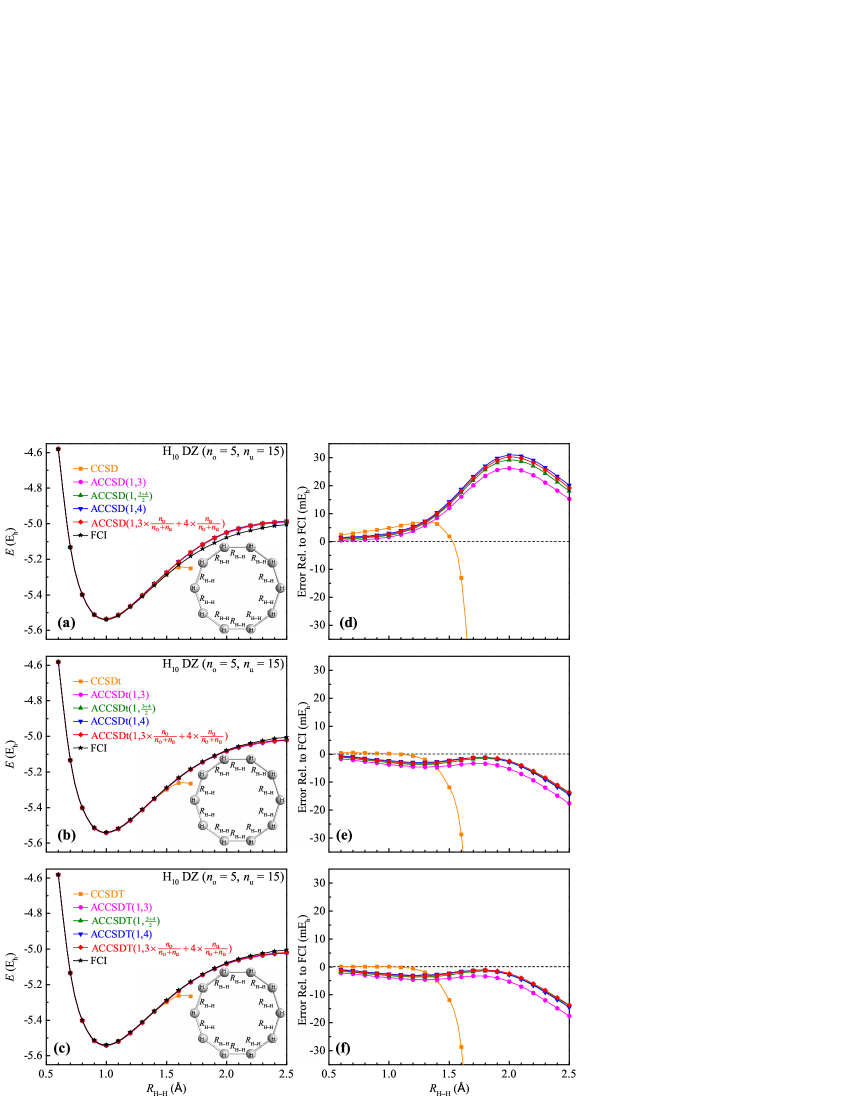
Figure 3: Ground-state PECs [panels (a)–(c)] and errors relative to FCI [panels (d)–(f)] for the symmetric dissociation of the $\text{H}_{10}$ ring resulting from the CCSD and various ACCSD [panels (a) and (d)], CCSDt and various ACCSDt [panels (b) and (e)], and CCSDT and various ACCSDT [panels (c) and (f)] calculations using the DZ basis set. The CCSDt and ACCSDt approaches employed a minimum active space consisting of five occupied and five lowest-energy unoccupied MOs that correlate with the 1$s$ shells of the individual hydrogen atoms. The FCI PEC included in panels (a)–(c) is shown to facilitate comparisons. Note that the CCSD, CCSDt, and CCSDT calculations failed to converge in the $R_{\text{H--H}}\geq 1.8$ Å region.

To further investigate the performance of the ACP methods, especially those that incorporate $T_{3}$ physics, in a strongly correlated regime coupled with non-trivial dynamical correlations, we studied the $D_{\text{10h}}$-symmetric dissociation of the $\text{H}_{10}$ ring, as described by the DZ basis set. The ground-state PECs of the $\text{H}_{10}$/DZ system resulting from the CCSD, CCSDt, and CCSDT calculations, the corresponding ACCSD, ACCSDt, and ACCSDT runs, and the exact FCI computations are shown in Tables 4–6 and Fig. 3. Table 4 summarizes the various CCSD-type calculations, including CCSD, ACCSD(1,3), $\text{ACCSD}(1{,}\tfrac{3+4}{2})$ = DCSD, $\text{ACCSD}(1{,}3\times\tfrac{n_{\text{o}}}{n_{\text{o}}+n_{\text{u}}}+4\times\tfrac{n_{\text{u}}}{n_{\text{o}}+n_{\text{u}}})$, and ACCSD(1,4). The results of the CCSDt, ACCSDt(1,3), $\text{ACCSDt}(1{,}\tfrac{3+4}{2})$, $\text{ACCSDt}(1{,}3\times\tfrac{n_{\text{o}}}{n_{\text{o}}+n_{\text{u}}}+4\times\tfrac{n_{\text{u}}}{n_{\text{o}}+n_{\text{u}}})$, and ACCSDt(1,4) computations are shown in Table 5. The CCSDT, ACCSDT(1,3), $\text{ACCSDT}(1{,}\tfrac{3+4}{2})$, $\text{ACCSDT}(1{,}3\times\tfrac{n_{\text{o}}}{n_{\text{o}}+n_{\text{u}}}+4\times\tfrac{n_{\text{u}}}{n_{\text{o}}+n_{\text{u}}})$, and ACCSDT(1,4) calculations are summarized in Table 6.

The symmetric dissociation of the $\text{H}_{10}$ system is more challenging than the previously discussed $\text{H}_{6}$ ring, since the ground electronic state of $\text{H}_{10}$, when all H–H distances are simultaneously stretched, involves the entanglement of 10 electrons, which is an increase in the number of strongly correlated electrons by two thirds. Because of the use of a smaller basis set, the dimension of the many-electron Hilbert space characterizing the $D_{\text{10h}}$-symmetric $\text{H}_{10}$/DZ system is smaller compared to $\text{H}_{6}$ using the cc-pVTZ basis [the number of the $S_{z}=0$ determinants of the $A_{g}(D_{\text{2h}})$ symmetry used in our FCI GAMESS calculations for the $\text{H}_{10}$/DZ system was 60,095,104, as opposed to 1,139,812,264 used for $\text{H}_{6}$/cc-pVTZ], but the challenge of strong correlations created by the simultaneous dissociation of all H–H bonds in the $\text{H}_{10}$ ring is more severe than in the case of its hexagonal $\text{H}_{6}$ cousin. This can be seen when examining the performance of the CCSD, CCSDt, and CCSDT approaches. As shown in Tables 4–6 and Fig. 3, the PECs resulting from the CCSD, CCSDt, and CCSDT calculations are not only incorrectly shaped, exhibiting an unphysical hump at the intermediate stretches of the H–H bonds, but they cannot be continued beyond $R_{\text{H--H}}\approx 1.7$ Å. The CCSDt and CCSDT methods reduce the $\sim$4–7 $\text{mE}_{\text{h}}$ errors relative to FCI obtained with the CCSD approach in the equilibrium ($R_{\text{H--H}}\approx 1.0$ Å) region to small fractions of a millihartree, but when $R_{\text{H--H}}>1.7$ Å, the CCSD, CCSDt, and CCSDT calculations diverge, even when initiated from the converged cluster amplitudes obtained at the neighboring geometries from the $R_{\text{H--H}}\leq 1.7$ Å region. As argued in Refs. Paldus et al. (1984a); Piecuch et al. (1990), using detailed mathematical analysis of the analytic properties of non-linear CC equations and the relevant numerical evidence, this is, most likely, caused by the existence of branch point singularities in the vicinity of the $R_{\text{H--H}}\approx 1.7$ Å geometry and the CCSD, CCSDt, and CCSDT solutions becoming complex when $R_{\text{H--H}}>1.7$ Å. The singularities and divergences of this kind were observed in the conventional CC calculations for the cyclic polyene models with 14 or more carbon sites Paldus et al. (1984a, b); Takahashi and Paldus (1985); Piecuch et al. (1990); Piecuch and Paldus (1991); Paldus and Piecuch (1992); Piecuch et al. (1992); Podeszwa et al. (2002), and we believe that our CCSD, CCSDt, and CCSDT computations for the $D_{\text{10h}}$-symmetric dissociation of the $\text{H}_{10}$ ring suffer from similar problems once the region of larger H–H separations is reached.

Tables 4–6 and Fig. 3 demonstrate that all ACP methods investigated in this work are capable of eliminating the singular behavior observed in the CCSD, CCSDt, and CCSDT calculations for the dissociating $\text{H}_{10}$ system. As was the case with the smaller $\text{H}_{\text{6}}$ ring, the ACCSD(1,3), $\text{ACCSD}(1{,}\tfrac{3+4}{2})$ = DCSD, $\text{ACCSD}(1{,}3\times\tfrac{n_{\text{o}}}{n_{\text{o}}+n_{\text{u}}}+4\times\tfrac{n_{\text{u}}}{n_{\text{o}}+n_{\text{u}}})$, and ACCSD(1,4) approaches and their ACCSDt and ACCSDT counterparts produce the qualitatively correct PECs that are in reasonable agreement with FCI, even when the H–H bonds in $\text{H}_{10}$ are significantly stretched. Although the DZ basis set used in our calculations for the $\text{H}_{10}$ system, in which $n_{\text{o}}=5$ and $n_{\text{u}}=15$, is much smaller than the cc-pVTZ basis used in the case of $\text{H}_{\text{6}}$, many of the accuracy patterns observed in the ACP computations for the $\text{H}_{\text{6}}$ ring apply to the symmetric dissociation of its ten-membered analog. For example, among the ACP schemes truncated at $T_{2}$ examined in this study, the ACCSD(1,3) method is most accurate and the ACCSD(1,4) approach performs worst, increasing the MUE and MSE values relative to FCI obtained with ACCSD(1,3), of 12.572 $\text{mE}_{\text{h}}$, to 15.505 $\text{mE}_{\text{h}}$ [see Table 4 and panels (a) and (d) in Fig. 3]. In analogy to the hexagonal $\text{H}_{\text{6}}$ system, the $\text{ACCSD}(1{,}\tfrac{3+4}{2})$ = DCSD and $\text{ACCSD}(1{,}3\times\tfrac{n_{\text{o}}}{n_{\text{o}}+n_{\text{u}}}+4\times\tfrac{n_{\text{u}}}{n_{\text{o}}+n_{\text{u}}})$ methods, which average the contributions from diagrams (3) and (4) of Fig. 1, produce the PECs located between the ACCSD(1,3) and ACCSD(1,4) ones. The $\text{ACCSD}(1{,}3\times\tfrac{n_{\text{o}}}{n_{\text{o}}+n_{\text{u}}}+4\times\tfrac{n_{\text{u}}}{n_{\text{o}}+n_{\text{u}}})$ PEC is closer to that obtained in the ACCSD(1,4) calculations, since the $\lambda$ factor entering Eqs. (6) and (12) used by $\text{ACCSD}(1{,}\tfrac{3+4}{2})$ is $\tfrac{1}{2}$, whereas the $\text{ACCSD}(1{,}3\times\tfrac{n_{\text{o}}}{n_{\text{o}}+n_{\text{u}}}+4\times\tfrac{n_{\text{u}}}{n_{\text{o}}+n_{\text{u}}})$ approach proposed in this work adopts the weighted average defined by $\lambda=\tfrac{n_{\text{o}}}{n_{\text{o}}+n_{\text{u}}}$, which in the case of the $\text{H}_{10}$/DZ system considered here corresponds to setting $\lambda$ at $\tfrac{1}{4}$, increasing the relative contribution of diagram (4) in Eqs. (6) and (12). Compared to the $\text{H}_{\text{6}}$/cc-pVTZ system, the differences among the ACCSD(1,3), $\text{ACCSD}(1{,}\tfrac{3+4}{2})$, $\text{ACCSD}(1{,}3\times\tfrac{n_{\text{o}}}{n_{\text{o}}+n_{\text{u}}}+4\times\tfrac{n_{\text{u}}}{n_{\text{o}}+n_{\text{u}}})$, and ACCSD(1,4) PECs corresponding to the symmetric dissociation of the $\text{H}_{10}$ ring are smaller, which is a consequence of the use of a smaller DZ basis set in the latter case [in the extreme limit of a minimum basis, where the p–h symmetry is approximately satisfied, the ACCSD(1,3), $\text{ACCSD}(1{,}\tfrac{3+4}{2})$, $\text{ACCSD}(1{,}3\times\tfrac{n_{\text{o}}}{n_{\text{o}}+n_{\text{u}}}+4\times\tfrac{n_{\text{u}}}{n_{\text{o}}+n_{\text{u}}})$, and ACCSD(1,4) results would be virtually identical], but the overall accuracy patterns characterizing the ACP methods with up to two-body clusters, especially the superior performance of the ACCSD(1,3) approximation, hold.

Because of the use of a smaller DZ basis in our calculations for the $\text{H}_{10}$ system, the similarities in the performance of the ACP methods using different ways of mixing diagrams (3) and (4) in Eqs. (6) and (12) are also observed at the ACCSDt and ACCSDT levels, but, as shown in Tables 5 and 6 and panels (b), (c), (e), and (f) of Fig. 3, the PECs resulting from the $\text{ACCSDt}(1{,}3\times\tfrac{n_{\text{o}}}{n_{\text{o}}+n_{\text{u}}}+4\times\tfrac{n_{\text{u}}}{n_{\text{o}}+n_{\text{u}}})$ and $\text{ACCSDT}(1{,}3\times\tfrac{n_{\text{o}}}{n_{\text{o}}+n_{\text{u}}}+4\times\tfrac{n_{\text{u}}}{n_{\text{o}}+n_{\text{u}}})$ calculations are most accurate when the H–H distances are larger. All of the ACP approaches with the connected triply excited clusters examined in this work, including ACCSDT(1,3), $\text{ACCSDT}(1{,}\tfrac{3+4}{2})$, $\text{ACCSDT}(1{,}3\times\tfrac{n_{\text{o}}}{n_{\text{o}}+n_{\text{u}}}+4\times\tfrac{n_{\text{u}}}{n_{\text{o}}+n_{\text{u}}})$, and ACCSDT(1,4) and their active-space ACCSDt(1,3), $\text{ACCSDt}(1{,}\tfrac{3+4}{2})$, $\text{ACCSDt}(1{,}3\times\tfrac{n_{\text{o}}}{n_{\text{o}}+n_{\text{u}}}+4\times\tfrac{n_{\text{u}}}{n_{\text{o}}+n_{\text{u}}})$, and ACCSDt(1,4) counterparts, offer major improvements in the underlying ACCSD(1,3), $\text{ACCSD}(1{,}\tfrac{3+4}{2})$ = DCSD, $\text{ACCSD}(1{,}3\times\tfrac{n_{\text{o}}}{n_{\text{o}}+n_{\text{u}}}+4\times\tfrac{n_{\text{u}}}{n_{\text{o}}+n_{\text{u}}})$, and ACCSD(1,4) results, reducing the MUE and MSE values relative to FCI by factors of $\sim$2–4, but, as in the case of the symmetric dissociation of the $\text{H}_{6}$ ring, the $\text{ACCSDt}(1{,}3\times\tfrac{n_{\text{o}}}{n_{\text{o}}+n_{\text{u}}}+4\times\tfrac{n_{\text{u}}}{n_{\text{o}}+n_{\text{u}}})$ and $\text{ACCSDT}(1{,}3\times\tfrac{n_{\text{o}}}{n_{\text{o}}+n_{\text{u}}}+4\times\tfrac{n_{\text{u}}}{n_{\text{o}}+n_{\text{u}}})$ methods perform best overall. Independent of the H–H separation, including the $R_{\text{H--H}}$ values as large as 2.5 Å (we recall that the equilibrium value of $R_{\text{H--H}}$ is about 1.0 Å), they reproduce the FCI correlation energies to within 1–2 % or about 3.8–3.9 $\text{mE}_{\text{h}}$ on average. If we limit ourselves to the $R_{\text{H--H}}=0.6\text{--}2.0$ Å region, the errors in the $\text{ACCSDt}(1{,}3\times\tfrac{n_{\text{o}}}{n_{\text{o}}+n_{\text{u}}}+4\times\tfrac{n_{\text{u}}}{n_{\text{o}}+n_{\text{u}}})$ and $\text{ACCSDT}(1{,}3\times\tfrac{n_{\text{o}}}{n_{\text{o}}+n_{\text{u}}}+4\times\tfrac{n_{\text{u}}}{n_{\text{o}}+n_{\text{u}}})$ energies relative to FCI are in the $\sim$1–3 $\text{mE}_{\text{h}}$ range. Given the dramatic failure and the singular behavior of the conventional CCSDt and CCSDT approaches and the MUE values characterizing the $\text{ACCSDt}(1{,}3\times\tfrac{n_{\text{o}}}{n_{\text{o}}+n_{\text{u}}}+4\times\tfrac{n_{\text{u}}}{n_{\text{o}}+n_{\text{u}}})$ and $\text{ACCSDT}(1{,}3\times\tfrac{n_{\text{o}}}{n_{\text{o}}+n_{\text{u}}}+4\times\tfrac{n_{\text{u}}}{n_{\text{o}}+n_{\text{u}}})$ calculations being 3–4 times smaller compared to ACCSD(1,3), $\text{ACCSD}(1{,}\tfrac{3+4}{2})$, $\text{ACCSD}(1{,}3\times\tfrac{n_{\text{o}}}{n_{\text{o}}+n_{\text{u}}}+4\times\tfrac{n_{\text{u}}}{n_{\text{o}}+n_{\text{u}}})$, and ACCSD(1,4), we are encouraged by the performance of the $\text{ACCSDt}(1{,}3\times\tfrac{n_{\text{o}}}{n_{\text{o}}+n_{\text{u}}}+4\times\tfrac{n_{\text{u}}}{n_{\text{o}}+n_{\text{u}}})$ and $\text{ACCSDT}(1{,}3\times\tfrac{n_{\text{o}}}{n_{\text{o}}+n_{\text{u}}}+4\times\tfrac{n_{\text{u}}}{n_{\text{o}}+n_{\text{u}}})$ schemes developed in this work. It is also encouraging that the unscaled ACCSDt(1,4) and ACCSDT(1,4) methods, which correspond to setting $\lambda$ in Eqs. (6) and (12) at 0 and which build upon the old ACCSD(1,4) approximation proposed in Ref. Piecuch and Paldus (1991) by incorporating $T_{3}$ correlations in it, are practically as accurate. In particular, they improve the results obtained with the $\text{ACCSDt}(1{,}\tfrac{3+4}{2})$ and $\text{ACCSDT}(1{,}\tfrac{3+4}{2})$ approaches, which extend the $\text{ACCSD}(1{,}\tfrac{3+4}{2})$ = DCSD scheme to the CCSDt/CCSDT-type treatments of the connected triples.

Last but not least, our calculations for the symmetric dissociation of the $\text{H}_{10}$ ring system summarized in Tables 5 and 6 and panels (b), (c), (e), and (f) confirm the previous observation that the active-space ACCSDt methods faithfully reproduce the corresponding ACCSDT energetics, even at larger H–H separations, at the small fraction of the computational cost. The differences between the ACCSDt(1,3), $\text{ACCSDt}(1{,}\tfrac{3+4}{2})$, $\text{ACCSDt}(1{,}3\times\tfrac{n_{\text{o}}}{n_{\text{o}}+n_{\text{u}}}+4\times\tfrac{n_{\text{u}}}{n_{\text{o}}+n_{\text{u}}})$, and ACCSDt(1,4) results and their respective ACCSDT(1,3), $\text{ACCSDT}(1{,}\tfrac{3+4}{2})$, $\text{ACCSDT}(1{,}3\times\tfrac{n_{\text{o}}}{n_{\text{o}}+n_{\text{u}}}+4\times\tfrac{n_{\text{u}}}{n_{\text{o}}+n_{\text{u}}})$, and ACCSDT(1,4) parents obtained for the $\text{H}_{10}$ system are smaller than in the case of the previously discussed $\text{H}_{6}$ ring, since the DZ basis set used in our calculations for $\text{H}_{10}$ is much smaller than the cc-pVTZ basis employed in the $\text{H}_{6}$ case and, as a consequence, the number of active unoccupied orbitals used in the ACCSDt calculations for the $\text{H}_{10}$/DZ system is a significant fraction (one third) of all unoccupied MOs, but we still see substantial reduction in the computational effort offered by the active-space treatment of triples compared to the corresponding ACCSDT levels, from 2 s per iteration on a single core of the aforementioned Dell node in the case of ACCSDT to 0.7 s in the ACCSDt case.

III.2 Symmetric Dissociation of the ${\text{H}}_{50}$ Linear Chain

Having analyzed the performance of the various ACP approaches, especially those incorporating the connected three-body clusters, in calculations for the symmetric dissociations of the six- and ten-membered hydrogen rings, we proceed to the examination of our final example, which is the $\text{H}_{50}$ linear chain. As in the case of the $\text{H}_{6}$ and $\text{H}_{10}$ systems discussed in Section III.1, we model the transition from the weakly correlated metallic regime in the equilibrium region, where the distances between the adjacent hydrogen atoms are around 1.8 bohr, to the strongly correlated insulator phase by simultaneously stretching all H–H bonds. Putting aside the periodic nature of the $\text{H}_{6}$ and $\text{H}_{10}$ ring structures, the main difference between the $\text{H}_{6}$ and $\text{H}_{10}$ clusters and the $\text{H}_{50}$ linear chain is a much larger number of the strongly correlated electrons in the latter system, which results in an enormous many-electron Hilbert space, spanned by $\sim 10^{27}$ singlet CSFs when the minimum basis set is employed and even larger numbers of CSFs when larger basis sets are considered. As already alluded to above, the exact Hamiltonian diagonalizations for the many-electron Hilbert spaces of such dimensionalities are outside reach of the best FCI algorithms and most powerful computer architectures available today, so in evaluating the performance of the ACP approaches considered in this work in calculations for the symmetric dissociation of the $\text{H}_{50}$ linear chain, we relied on the nearly exact PEC obtained in the LDMRG(500) computations using the STO-6G minimum basis set reported in Ref. Hachmann et al. (2006). Because of the use of the minimum basis, for which $n_{\rm o}=n_{\rm u}=N_{\rm o}=N_{\rm u}=25$, our ACCSDt and CCSDt calculations for the $\text{H}_{50}$ system are equivalent to their ACCSDT and CCSDT counterparts and the PECs obtained with the $\text{ACCSDT}(1{,}3\times\tfrac{n_{\text{o}}}{n_{\text{o}}+n_{\text{u}}}+4\times\tfrac{n_{\text{u}}}{n_{\text{o}}+n_{\text{u}}})$ = $\text{ACCSDT}(1{,}\tfrac{3+4}{2})$, ACCSDT(1,3), and ACCSDT(1,4) approaches are nearly identical, so in the discussion below we concentrate on the $\text{ACCSDT}(1{,}\tfrac{3+4}{2})$ results and the results generated with CCSD, CCSDT, and $\text{ACCSD}(1{,}\tfrac{3+4}{2})$ = DCSD. The DCSD calculations for the symmetric dissociation of the $\text{H}_{50}$ linear chain, as described by the STO-6G basis set, were also reported in Ref. Kats and Manby (2013), but the authors of Ref. Kats and Manby (2013) did not consider $T_{3}$ correlations in their work. Our computations for the $\text{H}_{50}$/STO-6G system discussed in this section allow us to investigate if the inclusion of the connected triply excited clusters via the $\text{ACCSDT}(1{,}\tfrac{3+4}{2})$ scheme implemented in this study can improve the DCSD PEC presented in Ref. Kats and Manby (2013).

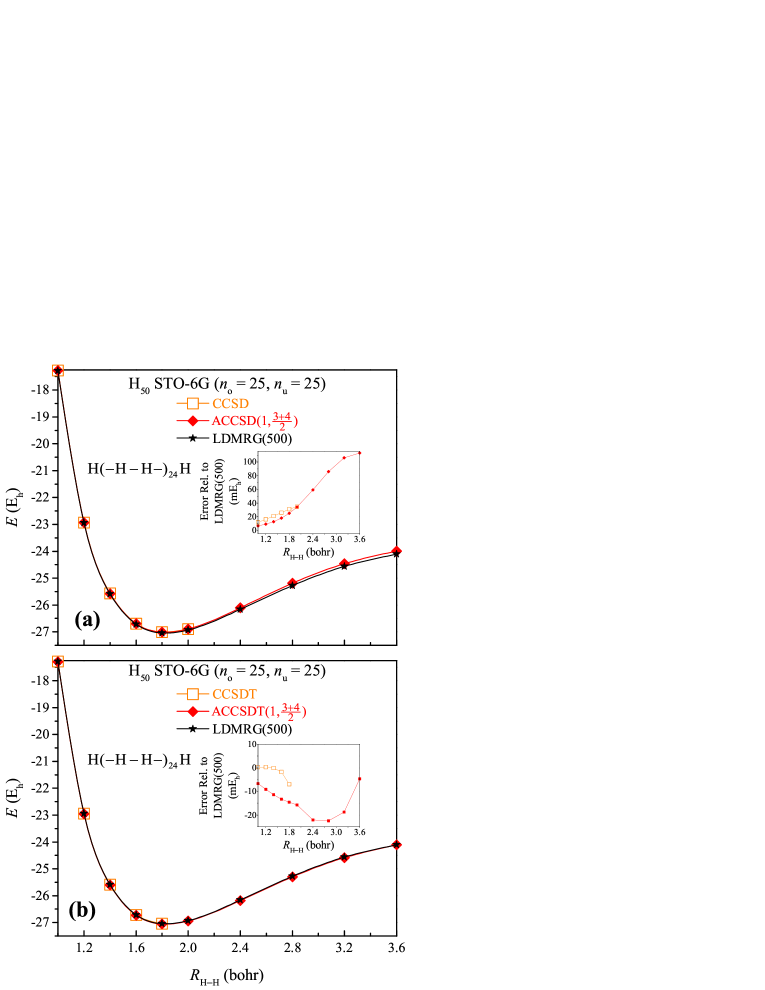
Figure 4: Ground-state PECs for the symmetric dissociation of the $\text{H}_{50}$ linear chain obtained in the (a) CCSD and $\text{ACCSD}(1{,}\tfrac{3+4}{2})$ and (b) CCSDT and $\text{ACCSDT}(1{,}\tfrac{3+4}{2})$ calculations using the STO-6G basis set. In this case $n_{\rm o}=n_{\rm u}=N_{\rm o}=N_{\rm u}$, so that $\text{ACCSD}(1{,}\tfrac{3+4}{2})$ = DCSD is equivalent to $\text{ACCSD}(1{,}3\times\tfrac{n_{\text{o}}}{n_{\text{o}}+n_{\text{u}}}+4\times\tfrac{n_{\text{u}}}{n_{\text{o}}+n_{\text{u}}})$ and $\text{ACCSDT}(1{,}\tfrac{3+4}{2})$ is equivalent to $\text{ACCSDt}(1{,}\tfrac{3+4}{2})$, $\text{ACCSDt}(1{,}3\times\tfrac{n_{\text{o}}}{n_{\text{o}}+n_{\text{u}}}+4\times\tfrac{n_{\text{u}}}{n_{\text{o}}+n_{\text{u}}})$, and $\text{ACCSDT}(1{,}3\times\tfrac{n_{\text{o}}}{n_{\text{o}}+n_{\text{u}}}+4\times\tfrac{n_{\text{u}}}{n_{\text{o}}+n_{\text{u}}})$. The LDMRG(500) PEC included for comparison purposes is based on the data reported in Ref. Hachmann et al. (2006). The insets show the errors relative to LDMRG(500). Note that the CCSD calculations failed to converge in the $R_{\text{H--H}}>2.0$ bohr region. We could not converge the CCSDT equations beyond $R_{\text{H--H}}=1.8$ bohr.

The information about the ground-state PECs corresponding to the symmetric dissociation of the $\text{H}_{50}$ linear chain, as described by the STO-6G basis, which resulted from our CCSD, CCSDT, $\text{ACCSD}(1{,}\tfrac{3+4}{2})$ = DCSD, and $\text{ACCSDT}(1{,}\tfrac{3+4}{2})$ calculations, along with the reference LDMRG(500) energetics taken from Ref. Hachmann et al. (2006), is summarized in Table 7 and Fig. 4. As one might anticipate, given the large number of strongly correlated electrons, the $\text{H}_{50}$ system is much more challenging than the previously discussed $\text{H}_{6}$ and $\text{H}_{10}$ rings. This becomes apparent when we look at the results of the CCSD and CCSDT calculations, which fail to converge already near the equilibrium region, most likely due to the emergence of branch point singularities and the real solutions of the corresponding amplitude equations becoming complex as all H–H bonds of the $\text{H}_{50}$ linear chain are simultaneously stretched. As pointed out in Section III.1, the singularities and divergences of this kind were observed in the studies of cyclic polyene models reported in Refs. Paldus et al. (1984a, b); Takahashi and Paldus (1985); Piecuch et al. (1990); Piecuch and Paldus (1991); Paldus and Piecuch (1992); Piecuch et al. (1992); Podeszwa et al. (2002). The fact that we could not converge the CCSD and CCSDT amplitudes for the $\text{H}_{50}$ system already in the equilibrium region is consistent with the observations made in Refs. Paldus et al. (1984a); Piecuch et al. (1990); Piecuch and Paldus (1991); Paldus and Piecuch (1992); Podeszwa et al. (2002) that the branch point singularities plaguing conventional CC calculations move toward the regions of weaker correlations as the system size increases. The CCSDT method offers significant improvements in the CCSD energies at compressed H–H distances, but this is not helpful, since neither CCSD nor CCSDT solutions can be continued beyond the equilibrium region.

In view of the above failures of the conventional CCSD and CCSDT approaches, it is encouraging to see that our $\text{ACCSDT}(1{,}\tfrac{3+4}{2})$ scheme provides a non-singular and reliable description of the $\text{H}_{50}$ linear chain in the entire range of H–H separations considered in this work, including the H–H bond lengths as large as twice the equilibrium value of $R_{\text{H--H}}$, reducing the MUE relative to the LDMRG(500) reference data that characterizes the already well-behaved $\text{ACCSD}(1{,}\tfrac{3+4}{2})$ = DCSD method, of more than 47 $\text{mE}_{\text{h}}$, to less than 14 $\text{mE}_{\text{h}}$ (see Table 7 and Fig. 4). The improvements in the results obtained with the lower-rank $\text{ACCSD}(1{,}\tfrac{3+4}{2})$ approach, which neglects $T_{3}$ contributions, offered by the $\text{ACCSDT}(1{,}\tfrac{3+4}{2})$ method, which includes them, are especially significant when $R_{\text{H--H}}\geq 2.0$ bohr, i.e., when the CCSDT calculations stop converging. While it is possible that the PEC representing the symmetric dissociation of the $\text{H}_{50}$ linear chain obtained with $\text{ACCSDT}(1{,}\tfrac{3+4}{2})$ starts behaving erratically when $R_{\text{H--H}}\gg 3.6$ bohr, the error reductions compared to $\text{ACCSD}(1{,}\tfrac{3+4}{2})$ in the strongly correlated $R_{\text{H--H}}=2.0\text{--}3.6$ bohr region, from about 34–113 $\text{mE}_{\text{h}}$ to 5–22 $\text{mE}_{\text{h}}$, are quite remarkable. The errors relative to the nearly exact LDMRG(500) data obtained in the $\text{ACCSDT}(1{,}\tfrac{3+4}{2})$ calculations for the $\text{H}_{50}$/STO-6G system are larger, in absolute value, than the errors relative to FCI characterizing the $\text{ACCSDT}(1{,}\tfrac{3+4}{2})$ and other ACCSDT computations for the $\text{H}_{6}$ and $\text{H}_{10}$ rings, but we have to keep in mind that $\text{H}_{50}$ is much larger than $\text{H}_{6}$ and $\text{H}_{10}$, so the errors relative to exact or nearly exact computations are expected to be larger too. What is more important is the observation that the $\text{ACCSDT}(1{,}\tfrac{3+4}{2})$ calculations for the dissociating $\text{H}_{50}$/STO-6G linear chain reproduce the LDMRG(500) correlation energies, which we use as a reference in this study, to within 1–2 %. This is a noticeable improvement over the underlying $\text{ACCSD}(1{,}\tfrac{3+4}{2})$ approach, which gives 2–5 % differences with the correlation energies obtained in the LDMRG(500) calculations reported in Ref. Hachmann et al. (2006). It is encouraging to observe that the $\text{ACCSDT}(1{,}\tfrac{3+4}{2})$ approach and most of the other methods in this category examined in this work, including $\text{ACCSDT}(1{,}3\times\tfrac{n_{\text{o}}}{n_{\text{o}}+n_{\text{u}}}+4\times\tfrac{n_{\text{u}}}{n_{\text{o}}+n_{\text{u}}})$ and ACCSDT(1,4) and their active-space variants, are capable of reproducing the exact or nearly exact correlation energies in the strongly correlated systems of the type of the hydrogen clusters discussed here and in Section III.1 to within 1–2 %, independent of the system size and size of the basis employed in the calculations, substantially improving the corresponding ACCSD computations. The $\text{ACCSDT}(1{,}\tfrac{3+4}{2})$ approach is more expensive than its lower-rank $\text{ACCSD}(1{,}\tfrac{3+4}{2})$ = DCSD counterpart, increasing 0.8 s per iteration on a single core of the Dell machine used in the present study to 482 s, when the $\text{H}_{50}$/STO-6G system is examined. We have to realize, however, that a few minutes per iteration on a single core for a system containing 50 strongly correlated electrons is an insignificant effort, given the observed improvements in the description of the corresponding PEC over CCSD, CCSDT, and $\text{ACCSD}(1{,}\tfrac{3+4}{2})$ offered by $\text{ACCSDT}(1{,}\tfrac{3+4}{2})$ in the region of stretched H–H distances, not to mention the fact that FCI calculations for $\text{H}_{50}$ are not feasible.

IV Conclusions

It is well established that the conventional single-reference CCSD, CCSDT, etc. hierarchy, in which the cluster operator $T$ is truncated at a given many-body rank, displays an erratic behavior when the number of strongly correlated electrons becomes larger than in typical multi-reference situations in chemistry involving single or double bond breaking. At the same time, traditional multi-reference approaches may become inapplicable due to the prohibitively large dimensionalities of the underlying multi-configurational model spaces when the numbers of active electrons and orbitals become larger. The ACP theories, in which one uses subsets of non-linear $(T_{2})^{2}$ diagrams in the CCD or CCSD amplitude equations, are capable of capturing strong correlations involving the entanglement of larger numbers of electrons, but they neglect the physics associated with the connected triply excited clusters needed for a more quantitative description. Furthermore, the specific combinations of $(T_{2})^{2}$ diagrams that work well in the strongly correlated regime of the minimum-basis-set model systems used in the past to rationalize the ACP methods may not necessarily be optimum when larger basis sets and more substantial dynamical correlations are involved. The objective of this study has been to examine both topics and suggest and test solutions that might help develop better and more quantitative ACP models in the future.

In this work, we dealt with the issue of the missing $T_{3}$ physics by combining the selected ACP schemes, including the previously formulated ACCSD(1,3), ACCSD(1,4), and $\text{ACCSD}(1{,}\tfrac{3+4}{2})$ = DCSD approaches and the novel $\text{ACCSD}(1{,}3\times\tfrac{n_{\text{o}}}{n_{\text{o}}+n_{\text{u}}}+4\times\tfrac{n_{\text{u}}}{n_{\text{o}}+n_{\text{u}}})$ methodology, in which diagrams (3) and (4) of Fig. 1 are scaled by factors depending on the numbers of occupied ($n_{\rm o}$) and unoccupied ($n_{\rm u}$) orbitals, with the idea of capturing the leading triply excited cluster amplitudes using active orbitals, which was previously exploited in the CCSDt and similar methods. The resulting ACCSDt(1,3), ACCSDt(1,4), $\text{ACCSDt}(1{,}\tfrac{3+4}{2})$, and $\text{ACCSDt}(1{,}3\times\tfrac{n_{\text{o}}}{n_{\text{o}}+n_{\text{u}}}+4\times\tfrac{n_{\text{u}}}{n_{\text{o}}+n_{\text{u}}})$ methods, which are obtained by considering the appropriate subsets of $(T_{2})^{2}$ diagrams in the amplitude equations projected on the doubly excited determinants within the CCSDt system, their more expensive ACCSDT(1,3), ACCSDT(1,4), $\text{ACCSDT}(1{,}\tfrac{3+4}{2})$, and $\text{ACCSDT}(1{,}3\times\tfrac{n_{\text{o}}}{n_{\text{o}}+n_{\text{u}}}+4\times\tfrac{n_{\text{u}}}{n_{\text{o}}+n_{\text{u}}})$ parents, in which $T_{3}$ component is treated fully, obtained from CCSDT, and the underlying ACCSD(1,3), ACCSD(1,4), $\text{ACCSD}(1{,}\tfrac{3+4}{2})$, and $\text{ACCSD}(1{,}3\times\tfrac{n_{\text{o}}}{n_{\text{o}}+n_{\text{u}}}+4\times\tfrac{n_{\text{u}}}{n_{\text{o}}+n_{\text{u}}})$ approximations were implemented and tested using the symmetric dissociations of the $\text{H}_{6}$ and $\text{H}_{10}$ rings, as described by the cc-pVTZ and DZ basis sets, and the $\text{H}_{50}$ linear chain treated with STO-6G. We used these three systems as our numerical examples, since the linear chains and rings of the equally spaced hydrogen atoms can be used to model metal–insulator transitions in which the weakly correlated metallic phase at compressed geometries becomes the strong correlated insulator at larger H–H separations. The $T_{3}$-corrected $\text{ACCSDt}(1{,}3\times\tfrac{n_{\text{o}}}{n_{\text{o}}+n_{\text{u}}}+4\times\tfrac{n_{\text{u}}}{n_{\text{o}}+n_{\text{u}}})$ and $\text{ACCSDT}(1{,}3\times\tfrac{n_{\text{o}}}{n_{\text{o}}+n_{\text{u}}}+4\times\tfrac{n_{\text{u}}}{n_{\text{o}}+n_{\text{u}}})$ schemes and their lower-rank $\text{ACCSD}(1{,}3\times\tfrac{n_{\text{o}}}{n_{\text{o}}+n_{\text{u}}}+4\times\tfrac{n_{\text{u}}}{n_{\text{o}}+n_{\text{u}}})$ counterpart, in which the connected triply excited clusters are neglected, were used to investigate if the $n_{\rm o}$- and $n_{\rm u}$-dependent scaling factors at diagrams (3) and (4) can help to improve accuracies when basis sets are larger than a minimum one. We gauged the performance of the various ACP schemes examined in this work by comparing the resulting PECs for the $\text{H}_{6}$/cc-pVTZ, $\text{H}_{10}$/DZ, and $\text{H}_{50}$/STO-6G systems with their exact, FCI ($\text{H}_{6}$/cc-pVTZ and $\text{H}_{10}$/DZ) or nearly exact, DMRG ($\text{H}_{50}$/STO-6G) counterparts. The FCI PECs for the symmetric dissociations of the $\text{H}_{6}$/cc-pVTZ and $\text{H}_{10}$/DZ ring systems were generated in this work using GAMESS. The reference PEC for the symmetric dissociation of the $\text{H}_{50}$ linear chain, as described by the STO-6G basis, was taken from Ref. Hachmann et al. (2006), where the authors used the LDMRG(500) approach. We also included the conventional CCSD, CCSDt, and CCSDT methods in our calculations.

We demonstrated that all ACP approaches examined in this study, without and with the connected triples, provide qualitatively correct PECs, eliminating the erratic and, in the case of $\text{H}_{10}$ and $\text{H}_{50}$, singular behavior of CCSD, CCSDt, and CCSDT in the strongly correlated regime. Of all ACP methods including $T_{3}$ correlations, the $\text{ACCSDt}(1{,}3\times\tfrac{n_{\text{o}}}{n_{\text{o}}+n_{\text{u}}}+4\times\tfrac{n_{\text{u}}}{n_{\text{o}}+n_{\text{u}}})$ approach and its $\text{ACCSDT}(1{,}3\times\tfrac{n_{\text{o}}}{n_{\text{o}}+n_{\text{u}}}+4\times\tfrac{n_{\text{u}}}{n_{\text{o}}+n_{\text{u}}})$ parent, which in the minimum-basis-set case become equivalent to $\text{ACCSDt}(1{,}\tfrac{3+4}{2})$ and $\text{ACCSDT}(1{,}\tfrac{3+4}{2})$, respectively, turned out to be overall most accurate, improving the corresponding $\text{ACCSD}(1{,}3\times\tfrac{n_{\text{o}}}{n_{\text{o}}+n_{\text{u}}}+4\times\tfrac{n_{\text{u}}}{n_{\text{o}}+n_{\text{u}}})$ [in the case of $\text{ACCSDt}(1{,}\tfrac{3+4}{2})$ and $\text{ACCSDT}(1{,}\tfrac{3+4}{2})$, $\text{ACCSD}(1{,}\tfrac{3+4}{2})$ = DCSD] PECs, especially in the regions of larger H–H separations, where correlations become stronger. In general, it was promising to find out that the $\text{ACCSDT}(1{,}3\times\tfrac{n_{\text{o}}}{n_{\text{o}}+n_{\text{u}}}+4\times\tfrac{n_{\text{u}}}{n_{\text{o}}+n_{\text{u}}})$, ACCSDT(1,4), and $\text{ACCSDT}(1{,}\tfrac{3+4}{2})$ methods and their more economical active-space $\text{ACCSDt}(1{,}3\times\tfrac{n_{\text{o}}}{n_{\text{o}}+n_{\text{u}}}+4\times\tfrac{n_{\text{u}}}{n_{\text{o}}+n_{\text{u}}})$, ACCSDt(1,4), and $\text{ACCSDt}(1{,}\tfrac{3+4}{2})$ counterparts reproduce the exact or nearly exact correlation energies in the hydrogen clusters, which model transitions from the weakly correlated metallic regime to the strongly correlated insulator phase, to within 1–2 %, reducing errors in the underlying ACCSD computations in a substantial manner. It was also encouraging to observe that all ACCSDt schemes, which use active orbitals that reflect on the nature of strong correlations of interest to identify the dominant $T_{3}$ contributions, faithfully reproduce the results of the corresponding ACCSDT calculations, in which the connected three-body clusters are treated fully, at the small fraction of the computational effort. While the $n_{\rm o}$- and $n_{\rm u}$-dependent scaling factors at diagrams (3) and (4) did not help the ACCSD calculations, they seem to be useful in improving the accuracies of the ACCSDt and ACCSDT computations when larger basis sets are employed. Having said this, there may be other, better ways of improving accuracies of $T_{3}$-corrected ACP approaches in calculations for strongly correlated systems involving the entanglement of larger numbers of electrons and using larger basis sets, and we will search for such ways in the future.

Among the other issues we would like to pursue is search for diagram cancellations within the externally corrected CCSDt and CCSDT amplitude equations projected on triples that would be consistent with the $(T_{2})^{2}$ diagram selections used by the ACP methods in the equations projected on doubles. While some diagram selections within the CCSDT equations were considered in Refs. Bartlett and Musiał (2006); Musiał and Bartlett (2007); Kats and Köhn (2019); Schraivogel and Kats (2021); Rishi and Valeev (2019), it remains unclear if the resulting or similar methods can handle strongly correlated systems involving the entanglement of larger numbers of electrons. As pointed out in Section II, model systems that were used in the past to justify the $(T_{2})^{2}$ diagram cancellations defining the ACP schemes by extracting $T_{4}$ contributions from the wave functions obtained by projecting out the singlet components of the UHF determinants breaking the $S^{2}$ symmetry, but not $S_{z}$, do not offer any guidance how to handle $T_{3}$ clusters, since the $T_{n}$ components with odd values of $n\geq 3$ are absent in the resulting PUHF states Paldus et al. (1984c); Piecuch et al. (1996a). In order to see the emergence of $T_{3}$ contributions through spin-symmetry breaking and restoration, one has to break the $S^{2}$ as well as $S_{z}$ symmetries, as in Ref. Henderson and Scuseria (2017). Thus, it would be worth examining if the considerations reported in Ref. Henderson and Scuseria (2017) allow one to come up with diagram cancellations or combinations within the CCSDt/CCSDT amplitude equations that could describe strong correlations, as understood throughout the present article, while accounting for the connected triply excited clusters at the same time.

Funding

This work has been supported by the Chemical Sciences, Geosciences and Biosciences Division, Office of Basic Energy Sciences, Office of Science, U.S. Department of Energy (Grant No. DE-FG02-01ER15228).

ORCID

Ilias Magoulas https://orcid.org/0000-0003-3252-9112
Jun Shen https://orcid.org/0000-0003-1838-3719
Piotr Piecuch https://orcid.org/0000-0002-7207-1815

Table 1: A comparison of the energies obtained with the CCSD and various ACCSD approaches with the exact FCI data for the symmetric dissociation of the $\text{H}_{6}$ ring, as described by the cc-pVTZ basis set, at selected bond distances between neighboring H atoms $R_{\text{H--H}}$ (in Å).

$R_{\text{H--H}}$	CCSD	ACCSD				FCI
		(1,3)	$(1,\tfrac{3+4}{2})$	$(1,3\times\tfrac{n_{\text{o}}}{n_{\text{o}}+n_{\text{u}}}+4\times\tfrac{n_{\text{u}}}{n_{\text{o}}+n_{\text{u}}})$	(1,4)
0.6	$3.422$	$-0.242$	$1.557$	$3.144$	$3.262$	$-2.858958$
0.7	$3.593$	$-0.320$	$1.618$	$3.321$	$3.448$	$-3.176147$
0.8	$3.823$	$-0.417$	$1.695$	$3.541$	$3.679$	$-3.331124$
0.9	$4.103$	$-0.534$	$1.788$	$3.809$	$3.959$	$-3.396176$
1.0	$4.424$	$-0.665$	$1.906$	$4.132$	$4.297$	$-3.410069$
1.1	$4.774$	$-0.805$	$2.059$	$4.522$	$4.705$	$-3.394673$
1.2	$5.139$	$-0.944$	$2.263$	$5.003$	$5.206$	$-3.362943$
1.3	$5.489$	$-1.068$	$2.543$	$5.608$	$5.833$	$-3.322850$
1.4	$5.758$	$-1.156$	$2.934$	$6.381$	$6.634$	$-3.279466$
1.5	$5.802$	$-1.175$	$3.479$	$7.377$	$7.662$	$-3.236119$
1.6	$5.309$	$-1.088$	$4.219$	$8.638$	$8.960$	$-3.195040$
1.7	$3.647$	$-0.865$	$5.165$	$10.165$	$10.529$	$-3.157716$
1.8	$-0.380$	$-0.508$	$6.266$	$11.872$	$12.280$	$-3.125051$
1.9	$-8.826$	$-0.071$	$7.388$	$13.563$	$14.012$	$-3.097433$
2.0	$-24.720$	$0.350$	$8.337$	$14.963$	$15.445$	$-3.074787$
2.1	$-51.331$	$0.660$	$8.931$	$15.813$	$16.314$	$-3.056686$
2.2	$-89.837$	$0.803$	$9.073$	$15.975$	$16.478$	$-3.042507$
2.3	$-137.197$	$0.782$	$8.776$	$15.463$	$15.951$	$-3.031571$
2.4	$-187.824$	$0.635$	$8.135$	$14.417$	$14.876$	$-3.023237$
2.5	$-237.074$	$0.416$	$7.277$	$13.027$	$13.447$	$-3.016948$
MUE	$39.624$	$0.675$	$4.770$	$9.037$	$9.349$	—
MSE	$-34.095$	$-0.311$	$4.770$	$9.037$	$9.349$	—

Table 2: A comparison of the energies obtained with the CCSDt and various ACCSDt approaches with the exact FCI data for the symmetric dissociation of the $\text{H}_{6}$ ring, as described by the cc-pVTZ basis set, at selected bond distances between neighboring H atoms $R_{\text{H--H}}$ (in Å).

$R_{\text{H--H}}$	CCSDt	ACCSDt				FCI
		(1,3)	$(1,\tfrac{3+4}{2})$	$(1,3\times\tfrac{n_{\text{o}}}{n_{\text{o}}+n_{\text{u}}}+4\times\tfrac{n_{\text{u}}}{n_{\text{o}}+n_{\text{u}}})$	(1,4)
0.6	$2.548$	$-1.234$	$0.615$	$2.243$	$2.365$	$-2.858958$
0.7	$2.419$	$-1.660$	$0.345$	$2.103$	$2.235$	$-3.176147$
0.8	$2.235$	$-2.247$	$-0.043$	$1.880$	$2.023$	$-3.331124$
0.9	$2.018$	$-2.962$	$-0.515$	$1.608$	$1.766$	$-3.396176$
1.0	$1.804$	$-3.757$	$-1.021$	$1.339$	$1.514$	$-3.410069$
1.1	$1.609$	$-4.592$	$-1.519$	$1.114$	$1.309$	$-3.394673$
1.2	$1.414$	$-5.454$	$-1.992$	$0.953$	$1.170$	$-3.362943$
1.3	$1.111$	$-6.428$	$-2.504$	$0.809$	$1.053$	$-3.322850$
1.4	$0.669$	$-7.437$	$-2.974$	$0.766$	$1.040$	$-3.279466$
1.5	$-0.074$	$-8.459$	$-3.375$	$0.855$	$1.163$	$-3.236119$
1.6	$-1.438$	$-9.451$	$-3.673$	$1.104$	$1.451$	$-3.195040$
1.7	$-4.014$	$-10.345$	$-3.837$	$1.516$	$1.904$	$-3.157716$
1.8	$-8.888$	$-11.062$	$-3.852$	$2.051$	$2.478$	$-3.125051$
1.9	$-17.983$	$-11.538$	$-3.744$	$2.611$	$3.069$	$-3.097433$
2.0	$-34.481$	$-11.755$	$-3.576$	$3.059$	$3.535$	$-3.074787$
2.1	$-62.336$	$-11.747$	$-3.432$	$3.266$	$3.744$	$-3.056686$
2.2	$-102.675$	$-11.583$	$-3.387$	$3.160$	$3.624$	$-3.042507$
2.3	$-150.692$	$-11.337$	$-3.483$	$2.735$	$3.172$	$-3.031571$
2.4	$-199.899$	$-11.068$	$-3.726$	$2.041$	$2.442$	$-3.023237$
2.5	$-246.321$	$-10.805$	$-4.094$	$1.154$	$1.516$	$-3.016948$
MUE	$42.231$	$7.746$	$2.585$	$1.818$	$2.129$	—
MSE	$-40.649$	$-7.746$	$-2.489$	$1.818$	$2.129$	—

Table 3: A comparison of the energies obtained with the CCSDT and various ACCSDT approaches with the exact FCI data for the symmetric dissociation of the $\text{H}_{6}$ ring, as described by the cc-pVTZ basis set, at selected bond distances between neighboring H atoms $R_{\text{H--H}}$ (in Å).

$R_{\text{H--H}}$	CCSDT	ACCSDT				FCI
		(1,3)	$(1,\tfrac{3+4}{2})$	$(1,3\times\tfrac{n_{\text{o}}}{n_{\text{o}}+n_{\text{u}}}+4\times\tfrac{n_{\text{u}}}{n_{\text{o}}+n_{\text{u}}})$	(1,4)
0.6	$0.079$	$-3.952$	$-1.996$	$-0.279$	$-0.151$	$-2.858958$
0.7	$0.095$	$-4.233$	$-2.123$	$-0.277$	$-0.139$	$-3.176147$
0.8	$0.116$	$-4.609$	$-2.304$	$-0.295$	$-0.146$	$-3.331124$
0.9	$0.140$	$-5.074$	$-2.530$	$-0.325$	$-0.162$	$-3.396176$
1.0	$0.160$	$-5.621$	$-2.792$	$-0.356$	$-0.175$	$-3.410069$
1.1	$0.166$	$-6.241$	$-3.079$	$-0.374$	$-0.174$	$-3.394673$
1.2	$0.137$	$-6.932$	$-3.381$	$-0.365$	$-0.143$	$-3.362943$
1.3	$0.031$	$-7.692$	$-3.686$	$-0.307$	$-0.059$	$-3.322850$
1.4	$-0.235$	$-8.512$	$-3.973$	$-0.172$	$0.106$	$-3.279466$
1.5	$-0.823$	$-9.369$	$-4.213$	$0.072$	$0.385$	$-3.236119$
1.6	$-2.046$	$-10.216$	$-4.371$	$0.457$	$0.808$	$-3.195040$
1.7	$-4.493$	$-10.982$	$-4.411$	$0.989$	$1.380$	$-3.157716$
1.8	$-9.245$	$-11.585$	$-4.316$	$1.631$	$2.061$	$-3.125051$
1.9	$-18.225$	$-11.959$	$-4.109$	$2.286$	$2.747$	$-3.097433$
2.0	$-34.617$	$-12.084$	$-3.855$	$2.817$	$3.296$	$-3.074787$
2.1	$-62.392$	$-11.995$	$-3.635$	$3.095$	$3.576$	$-3.056686$
2.2	$-102.685$	$-11.760$	$-3.526$	$3.048$	$3.514$	$-3.042507$
2.3	$-150.676$	$-11.452$	$-3.567$	$2.673$	$3.111$	$-3.031571$
2.4	$-199.857$	$-11.129$	$-3.764$	$2.019$	$2.421$	$-3.023237$
2.5	$-246.248$	$-10.820$	$-4.092$	$1.165$	$1.528$	$-3.016948$
MUE	$41.623$	$8.811$	$3.486$	$1.150$	$1.304$	—
MSE	$-41.531$	$-8.811$	$-3.486$	$0.875$	$1.189$	—

Table 4: A comparison of the energies obtained with the CCSD and various ACCSD approaches with the exact FCI data for the symmetric dissociation of the $\text{H}_{10}$ ring, as described by the DZ basis set, at selected bond distances between neighboring H atoms $R_{\text{H--H}}$ (in Å).

$R_{\text{H--H}}$	CCSD	ACCSD				FCI
		(1,3)	$(1,\tfrac{3+4}{2})$	$(1,3\times\tfrac{n_{\text{o}}}{n_{\text{o}}+n_{\text{u}}}+4\times\tfrac{n_{\text{u}}}{n_{\text{o}}+n_{\text{u}}})$	(1,4)
0.6	$2.461$	$0.412$	$0.945$	$1.204$	$1.458$	$-4.581177$
0.7	$2.942$	$0.498$	$1.071$	$1.348$	$1.619$	$-5.133564$
0.8	$3.519$	$0.708$	$1.314$	$1.606$	$1.890$	$-5.400721$
0.9	$4.157$	$1.053$	$1.689$	$1.992$	$2.285$	$-5.513021$
1.0	$4.878$	$1.591$	$2.265$	$2.582$	$2.886$	$-5.538852$
1.1	$5.691$	$2.435$	$3.164$	$3.501$	$3.821$	$-5.516586$
1.2	$6.510$	$3.744$	$4.552$	$4.917$	$5.257$	$-5.468944$
1.3	$7.013$	$5.701$	$6.620$	$7.022$	$7.388$	$-5.409818$
1.4	$6.288$	$8.451$	$9.520$	$9.972$	$10.370$	$-5.347723$
1.5	$1.896$	$11.987$	$13.258$	$13.773$	$14.209$	$-5.287756$
1.6	$-13.106$	$16.041$	$17.575$	$18.168$	$18.647$	$-5.232798$
1.7	$-66.276$	$20.069$	$21.930$	$22.618$	$23.144$	$-5.184271$
1.8	NC	$23.410$	$25.650$	$26.446$	$27.026$	$-5.142644$
1.9	NC	$25.531$	$28.163$	$29.075$	$29.715$	$-5.107796$
2.0	NC	$26.191$	$29.172$	$30.197$	$30.903$	$-5.079254$
2.1	NC	$25.462$	$28.691$	$29.809$	$30.585$	$-5.056349$
2.2	NC	$23.636$	$26.967$	$28.146$	$28.985$	$-5.038308$
2.3	NC	$21.090$	$24.372$	$25.568$	$26.453$	$-5.024332$
2.4	NC	$18.193$	$21.298$	$22.468$	$23.370$	$-5.013655$
2.5	NC	$15.248$	$18.087$	$19.193$	$20.080$	$-5.005591$
MUE	NA	$12.572$	$14.315$	$14.980$	$15.505$	—
MSE	NA	$12.572$	$14.315$	$14.980$	$15.505$	—

Table 5: A comparison of the energies obtained with the CCSDt and various ACCSDt approaches with the exact FCI data for the symmetric dissociation of the $\text{H}_{10}$ ring, as described by the DZ basis set, at selected bond distances between neighboring H atoms $R_{\text{H--H}}$ (in Å).

$R_{\text{H--H}}$	CCSDt	ACCSDt				FCI
		(1,3)	$(1,\tfrac{3+4}{2})$	$(1,3\times\tfrac{n_{\text{o}}}{n_{\text{o}}+n_{\text{u}}}+4\times\tfrac{n_{\text{u}}}{n_{\text{o}}+n_{\text{u}}})$	(1,4)
0.6	$0.455$	$-1.751$	$-1.181$	$-0.904$	$-0.633$	$-4.581177$
0.7	$0.554$	$-2.110$	$-1.502$	$-1.209$	$-0.922$	$-5.133564$
0.8	$0.416$	$-2.726$	$-2.081$	$-1.773$	$-1.473$	$-5.400721$
0.9	$0.349$	$-3.218$	$-2.541$	$-2.221$	$-1.912$	$-5.513021$
1.0	$0.181$	$-3.735$	$-3.019$	$-2.686$	$-2.369$	$-5.538852$
1.1	$-0.084$	$-4.169$	$-3.399$	$-3.050$	$-2.724$	$-5.516586$
1.2	$-0.650$	$-4.477$	$-3.634$	$-3.266$	$-2.933$	$-5.468944$
1.3	$-1.956$	$-4.591$	$-3.654$	$-3.266$	$-2.931$	$-5.409818$
1.4	$-4.961$	$-4.457$	$-3.399$	$-2.994$	$-2.672$	$-5.347723$
1.5	$-11.879$	$-4.091$	$-2.881$	$-2.468$	$-2.182$	$-5.287756$
1.6	$-28.679$	$-3.630$	$-2.233$	$-1.824$	$-1.609$	$-5.232798$
1.7	$-81.643$	$-3.315$	$-1.692$	$-1.300$	$-1.193$	$-5.184271$
1.8	NC	$-3.398$	$-1.510$	$-1.144$	$-1.178$	$-5.142644$
1.9	NC	$-4.043$	$-1.862$	$-1.523$	$-1.712$	$-5.107796$
2.0	NC	$-5.295$	$-2.810$	$-2.494$	$-2.832$	$-5.079254$
2.1	NC	$-7.106$	$-4.333$	$-4.029$	$-4.497$	$-5.056349$
2.2	NC	$-9.380$	$-6.355$	$-6.055$	$-6.626$	$-5.038308$
2.3	NC	$-12.001$	$-8.762$	$-8.462$	$-9.114$	$-5.024332$
2.4	NC	$-14.806$	$-11.381$	$-11.083$	$-11.806$	$-5.013655$
2.5	NC	$-17.551$	$-13.966$	$-13.660$	$-14.471$	$-5.005591$
MUE	NA	$5.793$	$4.110$	$3.770$	$3.790$	—
MSE	NA	$-5.793$	$-4.110$	$-3.770$	$-3.790$	—

Table 6: A comparison of the energies obtained with the CCSDT and various ACCSDT approaches with the exact FCI data for the symmetric dissociation of the $\text{H}_{10}$ ring, as described by the DZ basis set, at selected bond distances between neighboring H atoms $R_{\text{H--H}}$ (in Å).

$R_{\text{H--H}}$	CCSDT	ACCSDT				FCI
		(1,3)	$(1,\tfrac{3+4}{2})$	$(1,3\times\tfrac{n_{\text{o}}}{n_{\text{o}}+n_{\text{u}}}+4\times\tfrac{n_{\text{u}}}{n_{\text{o}}+n_{\text{u}}})$	(1,4)
0.6	$0.065$	$-2.167$	$-1.591$	$-1.311$	$-1.037$	$-4.581177$
0.7	$0.094$	$-2.602$	$-1.986$	$-1.688$	$-1.398$	$-5.133564$
0.8	$0.110$	$-3.054$	$-2.404$	$-2.093$	$-1.790$	$-5.400721$
0.9	$0.101$	$-3.485$	$-2.805$	$-2.482$	$-2.172$	$-5.513021$
1.0	$0.035$	$-3.894$	$-3.175$	$-2.841$	$-2.523$	$-5.538852$
1.1	$-0.170$	$-4.262$	$-3.491$	$-3.141$	$-2.815$	$-5.516586$
1.2	$-0.703$	$-4.535$	$-3.691$	$-3.323$	$-2.989$	$-5.468944$
1.3	$-1.991$	$-4.631$	$-3.693$	$-3.305$	$-2.969$	$-5.409818$
1.4	$-4.986$	$-4.487$	$-3.428$	$-3.023$	$-2.700$	$-5.347723$
1.5	$-11.897$	$-4.115$	$-2.904$	$-2.490$	$-2.205$	$-5.287756$
1.6	$-28.687$	$-3.649$	$-2.251$	$-1.842$	$-1.626$	$-5.232798$
1.7	$-81.631$	$-3.330$	$-1.706$	$-1.313$	$-1.206$	$-5.184271$
1.8	NC	$-3.408$	$-1.520$	$-1.153$	$-1.187$	$-5.142644$
1.9	NC	$-4.049$	$-1.867$	$-1.528$	$-1.717$	$-5.107796$
2.0	NC	$-5.296$	$-2.811$	$-2.494$	$-2.833$	$-5.079254$
2.1	NC	$-7.101$	$-4.329$	$-4.025$	$-4.493$	$-5.056349$
2.2	NC	$-9.371$	$-6.346$	$-6.045$	$-6.618$	$-5.038308$
2.3	NC	$-11.988$	$-8.750$	$-8.449$	$-9.100$	$-5.024332$
2.4	NC	$-14.790$	$-11.365$	$-11.068$	$-11.791$	$-5.013655$
2.5	NC	$-17.533$	$-13.927$	$-13.644$	$-14.459$	$-5.005591$
MUE	NA	$5.887$	$4.202$	$3.863$	$3.881$	—
MSE	NA	$-5.887$	$-4.202$	$-3.863$	$-3.881$	—

Table 7: A comparison of the energies obtained with the CCSD, $\text{ACCSD}(1{,}\tfrac{3+4}{2})$ = DCSD, CCSDT, and $\text{ACCSDT}(1{,}\tfrac{3+4}{2})$ approaches with the nearly exact LDMRG(500) data for the symmetric dissociation of the $\text{H}_{50}$ linear chain, as described by the STO-6G basis set, at selected bond distances between neighboring H atoms $R_{\text{H--H}}$ (in bohr).

$R_{\text{H--H}}$	CCSD	$\text{ACCSD}(1{,}\tfrac{3+4}{2})$	CCSDT	$\text{ACCSDT}(1{,}\tfrac{3+4}{2})$	LDMRG(500)
1.0	$11.90$	$6.30$	$0.27$	$-6.68$	$-17.28407$
1.2	$16.28$	$9.12$	$0.29$	$-9.08$	$-22.94765$
1.4	$20.99$	$12.78$	$-0.10$	$-11.37$	$-25.59378$
1.6	$26.01$	$17.82$	$-1.71$	$-13.26$	$-26.71944$
1.8	$31.00$	$24.87$	$-6.96$	$-14.62$	$-27.03865$
2.0	$34.60$	$34.30$	NC	$-15.73$	$-26.92609$
2.4	NC	$59.23$	NC	$-22.04$	$-26.16057$
2.8	NC	$86.24$	NC	$-22.47$	$-25.27480$
3.2	NC	$106.45$	NC	$-18.78$	$-24.56828$
3.6	NC	$113.43$	NC	$-4.66$	$-24.10277$
MUE	NA	$47.05$	NA	$13.87$	—
MSE	NA	$47.05$	NA	$-13.87$	—

Figure 1: Goldstone–Brandow orbital diagrams for the $(T_{2})^{2}$ contributions $\Lambda_{k}^{(2)}(AB,IJ;S_{r})$, $k=1\text{--}5$, to the CCD or CCSD equations projected on the singlet pp–hh coupled orthogonally spin-adapted doubly excited $\ket{\Phi_{IJ}^{AB}}_{S_{r}}$ states. The intermediate spin quantum number $S_{r}$ in the definition of the $\ket{\Phi_{IJ}^{AB}}_{S_{r}}$ states and the associated doubly excited cluster amplitudes $t_{AB}^{IJ}(S_{r})$ in the definition of the orthogonally spin-adapted $T_{2}$ operators, represented by the Brandow-type, oval-shaped vertices, is 0 or 1. The occupied orbital indices $M$ and $N$, the unoccupied orbital indices $E$ and $F$, and the intermediate spin quantum numbers $\widetilde{S}_{r}$ and $\widetilde{S}_{r}^{\prime}$ are summed over. The ${\mathscr{S}}_{AB}=1+(AB)$ and ${\mathscr{S}}_{IJ}=1+(IJ)$ operators at the diagrams are index symmetrizers that translate into the symmetrizers or antisymmetrizers, ${\mathscr{S}}_{AB}(S_{r})=1+(-1)^{S_{r}}(AB)$ and ${\mathscr{S}}_{IJ}(S_{r})=1+(-1)^{S_{r}}(IJ)$, respectively, in the resulting algebraic expressions.

References

- Hubbard (1957) J. Hubbard, Proc. R. Soc. London A 240, 539 (1957).
- Hugenholtz (1957) N. M. Hugenholtz, Physica 23, 481 (1957).
- Coester (1958) F. Coester, Nucl. Phys. 7, 421 (1958).
- Coester and Kümmel (1960) F. Coester and H. Kümmel, Nucl. Phys. 17, 477 (1960).
- Čížek (1966a) J. Čížek, J. Chem. Phys. 45, 4256 (1966a).
- Čížek (1969) J. Čížek, Adv. Chem. Phys. 14, 35 (1969).
- Čížek and Paldus (1971) J. Čížek and J. Paldus, Int. J. Quantum Chem. 5, 359 (1971).
- Paldus et al. (1972) J. Paldus, J. Čížek, and I. Shavitt, Phys. Rev. A 5, 50 (1972).
- Paldus and Li (1999) J. Paldus and X. Li, Adv. Chem. Phys. 110, 1 (1999).
- Bartlett and Musiał (2007) R. J. Bartlett and M. Musiał, Rev. Mod. Phys. 79, 291 (2007).
- Purvis and Bartlett (1982) G. D. Purvis, III and R. J. Bartlett, J. Chem. Phys. 76, 1910 (1982).
- Cullen and Zerner (1982) J. M. Cullen and M. C. Zerner, J. Chem. Phys. 77, 4088 (1982).
- Scuseria et al. (1987) G. E. Scuseria, A. C. Scheiner, T. J. Lee, J. E. Rice, and H. F. Schaefer, III, J. Chem. Phys. 86, 2881 (1987).
- Piecuch and Paldus (1989) P. Piecuch and J. Paldus, Int. J. Quantum Chem. 36, 429 (1989).
- Noga and Bartlett (1987) J. Noga and R. J. Bartlett, J. Chem. Phys. 86, 7041 (1987), ibid. 89, 3401 (1988) [Erratum].
- Scuseria and Schaefer (1988) G. E. Scuseria and H. F. Schaefer, III, Chem. Phys. Lett. 152, 382 (1988).
- Watts and Bartlett (1990) J. D. Watts and R. J. Bartlett, J. Chem. Phys. 93, 6104 (1990).
- Oliphant and Adamowicz (1991a) N. Oliphant and L. Adamowicz, J. Chem. Phys. 95, 6645 (1991a).
- Kucharski and Bartlett (1991) S. A. Kucharski and R. J. Bartlett, Theor. Chim. Acta 80, 387 (1991).
- Kucharski and Bartlett (1992) S. A. Kucharski and R. J. Bartlett, J. Chem. Phys. 97, 4282 (1992).
- Piecuch and Adamowicz (1994a) P. Piecuch and L. Adamowicz, J. Chem. Phys. 100, 5792 (1994a).
- Emrich (1981) K. Emrich, Nucl. Phys. A 351, 379 (1981).
- Geertsen et al. (1989) J. Geertsen, M. Rittby, and R. J. Bartlett, Chem. Phys. Lett. 164, 57 (1989).
- Stanton and Bartlett (1993) J. F. Stanton and R. J. Bartlett, J. Chem. Phys. 98, 7029 (1993).
- Kowalski and Piecuch (2001a) K. Kowalski and P. Piecuch, J. Chem. Phys. 115, 643 (2001a).
- Kowalski and Piecuch (2001b) K. Kowalski and P. Piecuch, Chem. Phys. Lett. 347, 237 (2001b).
- Kucharski et al. (2001) S. A. Kucharski, M. Włoch, M. Musiał, and R. J. Bartlett, J. Chem. Phys. 115, 8263 (2001).
- Kállay and Gauss (2004) M. Kállay and J. Gauss, J. Chem. Phys. 121, 9257 (2004).
- Hirata (2004) S. Hirata, J. Chem. Phys. 121, 51 (2004).
- Monkhorst (1977) H. Monkhorst, Int. J. Quantum Chem. Symp. 11, 421 (1977).
- Dalgaard and Monkhorst (1983) E. Dalgaard and H. Monkhorst, Phys. Rev. A 28, 1217 (1983).
- Mukherjee and Mukherjee (1979) D. Mukherjee and P. K. Mukherjee, Chem. Phys. 39, 325 (1979).
- Sekino and Bartlett (1984) H. Sekino and R. J. Bartlett, Int. J. Quantum Chem. Symp. 18, 255 (1984).
- Takahashi and Paldus (1986) M. Takahashi and J. Paldus, J. Chem. Phys. 85, 1486 (1986).
- Koch and Jørgensen (1990) H. Koch and P. Jørgensen, J. Chem. Phys. 93, 3333 (1990).
- Koch et al. (1990) H. Koch, H. J. A. Jensen, P. Jørgensen, and T. Helgaker, J. Chem. Phys. 93, 3345 (1990).
- Kondo et al. (1995) A. E. Kondo, P. Piecuch, and J. Paldus, J. Chem. Phys. 102, 6511 (1995).
- Kondo et al. (1996) A. E. Kondo, P. Piecuch, and J. Paldus, J. Chem. Phys. 104, 8566 (1996).
- Mott (1949) N. F. Mott, Proc. Phys. Soc. A 62, 416 (1949).
- Mott (1968) N. F. Mott, Rev. Mod. Phys. 40, 677 (1968).
- Mott (1990) N. F. Mott, Metal-Insulator Transitions (Taylor and Francis, London, 1974; 2nd edition 1990, 1990).
- Hubbard (1963) J. Hubbard, Proc. R. Soc. London A 276, 238 (1963).
- Hubbard (1964a) J. Hubbard, Proc. R. Soc. London A 277, 237 (1964a).
- Hubbard (1964b) J. Hubbard, Proc. R. Soc. London A 281, 401 (1964b).
- Vollhardt (1984) D. Vollhardt, Rev. Mod. Phys. 56, 99 (1984).
- Imada et al. (1998) M. Imada, A. Fujimori, and Y. Tokura, Rev. Mod. Phys. 70, 1039 (1998).
- Hachmann et al. (2006) J. Hachmann, W. Cardoen, and G. K.-L. Chan, J. Chem. Phys. 125, 144101 (2006).
- Bendazzoli et al. (2011) G. L. Bendazzoli, S. Evangelisti, and A. Monari, Int. J. Quantum Chem. 111, 3416 (2011).
- Motta et al. (2017) M. Motta, D. M. Ceperley, G. K.-L. Chan, J. A. Gomez, E. Gull, S. Guo, C. A. Jiménez-Hoyos, T. N. Lan, J. Li, F. Ma, A. J. Millis, N. V. Prokof’ev, U. Ray, G. E. Scuseria, S. Sorella, E. M. Stoudenmire, Q. Sun, I. S. Tupitsyn, S. R. White, D. Zgid, and S. Zhang, Phys. Rev. X 7, 031059 (2017).
- Tsuchimochi and Scuseria (2009) T. Tsuchimochi and G. E. Scuseria, J. Chem. Phys. 131, 121102 (2009).
- Sinitskiy et al. (2010) A. V. Sinitskiy, L. Greenman, and D. A. Mazziotti, J. Chem. Phys. 133, 014104 (2010).
- Kats and Manby (2013) D. Kats and F. R. Manby, J. Chem. Phys. 139, 021102 (2013).
- Pastorczak et al. (2017) E. Pastorczak, J. Shen, M. Hapka, P. Piecuch, and K. Pernal, J. Chem. Theory Comput. 13, 5404 (2017).
- Stair and Evangelista (2020) N. H. Stair and F. A. Evangelista, J. Chem. Phys. 153, 104108 (2020).
- Pauncz et al. (1962a) R. Pauncz, J. de Heer, and P.-O. Löwdin, J. Chem. Phys. 36, 2247 (1962a).
- Pauncz et al. (1962b) R. Pauncz, J. de Heer, and P.-O. Löwdin, J. Chem. Phys. 36, 2257 (1962b).
- Pariser and Parr (1953a) R. Pariser and R. G. Parr, J. Chem. Phys. 21, 466 (1953a).
- Pariser and Parr (1953b) R. Pariser and R. G. Parr, J. Chem. Phys. 21, 767 (1953b).
- Pople (1953) J. A. Pople, Trans. Faraday Soc. 49, 1375 (1953).
- Paldus et al. (1984a) J. Paldus, M. Takahashi, and R. W. H. Cho, Phys. Rev. B 30, 4267 (1984a).
- Paldus et al. (1984b) J. Paldus, M. Takahashi, and R. W. H. Cho, Int. J. Quantum Chem. Symp. 18, 237 (1984b).
- Takahashi and Paldus (1985) M. Takahashi and J. Paldus, Phys. Rev. B 31, 5121 (1985).
- Piecuch et al. (1990) P. Piecuch, S. Zarrabian, J. Paldus, and J. Čížek, Phys. Rev. B 42, 3351 (1990).
- Piecuch and Paldus (1991) P. Piecuch and J. Paldus, Int. J. Quantum Chem. Symp. 25, 9 (1991).
- Paldus and Piecuch (1992) J. Paldus and P. Piecuch, Int. J. Quantum Chem. 42, 135 (1992).
- Piecuch et al. (1992) P. Piecuch, J. Čížek, and J. Paldus, Int. J. Quantum Chem. 42, 165 (1992).
- Podeszwa et al. (2002) R. Podeszwa, S. A. Kucharski, and L. Z. Stolarczyk, J. Chem. Phys. 116, 480 (2002).
- Lindgren and Mukherjee (1987) I. Lindgren and D. Mukherjee, Phys. Rep. 151, 93 (1987).
- Piecuch and Kowalski (2002) P. Piecuch and K. Kowalski, Int. J. Mol. Sci. 3, 676 (2002).
- Lyakh et al. (2012) D. I. Lyakh, M. Musiał, V. F. Lotrich, and R. J. Bartlett, Chem. Rev. 112, 182 (2012).
- Evangelista (2018) F. A. Evangelista, J. Chem. Phys. 149, 030901 (2018).
- Szalay et al. (2012) P. G. Szalay, T. Müller, G. Gidofalvi, H. Lischka, and R. Shepard, Chem. Rev. 112, 108 (2012).
- Roca-Sanjuán et al. (2012) D. Roca-Sanjuán, F. Aquilante, and R. Lindh, WIREs Comput. Mol. Sci. 2, 585 (2012).
- Chattopadhyay et al. (2016) S. Chattopadhyay, R. K. Chaudhuri, U. S. Mahapatra, A. Ghosh, and S. S. Ray, WIREs Comput. Mol. Sci. 6, 266 (2016).
- Ruedenberg et al. (1982) K. Ruedenberg, M. W. Schmidt, M. M. Gilbert, and S. T. Elbert, Chem. Phys. 71, 41 (1982).
- Roos (1987) B. O. Roos, Adv. Chem. Phys. 69, 399 (1987).
- White (1992) S. R. White, Phys. Rev. Lett. 69, 2863 (1992).
- White and Martin (1999) S. R. White and R. L. Martin, J. Chem. Phys. 110, 4127 (1999).
- Mitrushenkov et al. (2001) A. O. Mitrushenkov, G. Fano, F. Ortolani, R. Linguerri, and P. Palmieri, J. Chem. Phys. 115, 6815 (2001).
- Chan and Head-Gordon (2002) G. K.-L. Chan and M. Head-Gordon, J. Chem. Phys. 116, 4462 (2002).
- Chan and Sharma (2011) G. K.-L. Chan and S. Sharma, Annu. Rev. Phys. Chem. 62, 465 (2011).
- Keller et al. (2015) S. Keller, M. Dolfi, M. Troyer, and M. Reiher, J. Chem. Phys. 143, 244118 (2015).
- Chan et al. (2016) G. K.-L. Chan, A. Keselman, N. Nakatani, Z. Li, and S. R. White, J. Chem. Phys. 145, 014102 (2016).
- Baiardi and Reiher (2020) A. Baiardi and M. Reiher, J. Chem. Phys. 152, 040903 (2020).
- Booth et al. (2009) G. H. Booth, A. J. W. Thom, and A. Alavi, J. Chem. Phys. 131, 054106 (2009).
- Cleland et al. (2010) D. Cleland, G. H. Booth, and A. Alavi, J. Chem. Phys. 132, 041103 (2010).
- Dobrautz et al. (2019) W. Dobrautz, S. D. Smart, and A. Alavi, J. Chem. Phys. 151, 094104 (2019).
- Ghanem et al. (2019) K. Ghanem, A. Y. Lozovoi, and A. Alavi, J. Chem. Phys. 151, 224108 (2019).
- Ghanem et al. (2020) K. Ghanem, K. Guther, and A. Alavi, J. Chem. Phys. 153, 224115 (2020).
- Whitten and Hackmeyer (1969) J. L. Whitten and M. Hackmeyer, J. Chem. Phys. 51, 5584 (1969).
- Bender and Davidson (1969) C. F. Bender and E. R. Davidson, Phys. Rev. 183, 23 (1969).
- Huron et al. (1973) B. Huron, J.-P. Malrieu, and P. Rancurel, J. Chem. Phys. 58, 5745 (1973).
- Buenker and Peyerimhoff (1974) R. J. Buenker and S. D. Peyerimhoff, Theor. Chim. Acta 35, 33 (1974).
- Schriber and Evangelista (2016) J. B. Schriber and F. A. Evangelista, J. Chem. Phys. 144, 161106 (2016).
- Schriber and Evangelista (2017) J. B. Schriber and F. A. Evangelista, J. Chem. Theory Comput. 13, 5354 (2017).
- Tubman et al. (2016) N. M. Tubman, J. Lee, T. Y. Takeshita, M. Head-Gordon, and K. B. Whaley, J. Chem. Phys. 145, 044112 (2016).
- Tubman et al. (2020) N. M. Tubman, C. D. Freeman, D. S. Levine, D. Hait, M. Head-Gordon, and K. B. Whaley, J. Chem. Theory Comput. 16, 2139 (2020).
- Liu and Hoffmann (2016) W. Liu and M. R. Hoffmann, J. Chem. Theory Comput. 12, 1169 (2016), ibid. 12, 3000 (2016) [Erratum].
- Zhang et al. (2020) N. Zhang, W. Liu, and M. R. Hoffmann, J. Chem. Theory Comput. 16, 2296 (2020).
- Holmes et al. (2016) A. A. Holmes, N. M. Tubman, and C. J. Umrigar, J. Chem. Theory Comput. 12, 3674 (2016).
- Sharma et al. (2017) S. Sharma, A. A. Holmes, G. Jeanmairet, A. Alavi, and C. J. Umrigar, J. Chem. Theory Comput. 13, 1595 (2017).
- Li et al. (2018) J. Li, M. Otten, A. A. Holmes, S. Sharma, and C. J. Umrigar, J. Chem. Phys. 149, 214110 (2018).
- Garniron et al. (2017) Y. Garniron, A. Scemama, P.-F. Loos, and M. Caffarel, J. Chem. Phys. 147, 034101 (2017).
- Garniron et al. (2019) Y. Garniron, T. Applencourt, K. Gasperich, A. Benali, A. Ferte, J. Paquier, B. Pradines, R. Assaraf, P. Reinhardt, J. Toulouse, P. Barbaresco, N. Renon, G. David, J.-P. Malrieu, M. Veril, M. Caffarel, P.-F. Loos, E. Giner, and A. Scemama, J. Chem. Theory Comput. 15, 3591 (2019).
- Malmqvist et al. (1990) P. A. Malmqvist, A. Rendell, and B. O. Roos, J. Phys. Chem. 94, 5477 (1990).
- Ivanic (2003a) J. Ivanic, J. Chem. Phys. 119, 9364 (2003a).
- Ivanic (2003b) J. Ivanic, J. Chem. Phys. 119, 9377 (2003b).
- Ma et al. (2011) D. Ma, G. Li Manni, and L. Gagliardi, J. Chem. Phys. 135, 044128 (2011).
- Vogiatzis et al. (2015) K. D. Vogiatzis, G. Li Manni, S. J. Stoneburner, D. Ma, and L. Gagliardi, J. Chem. Theory Comput. 11, 3010 (2015).
- Hermes and Gagliardi (2019) M. R. Hermes and L. Gagliardi, J. Chem. Theory Comput. 15, 972 (2019).
- Kurashige and Yanai (2011) Y. Kurashige and T. Yanai, J. Chem. Phys. 135, 094104 (2011).
- Guo et al. (2016) S. Guo, M. A. Watson, W. Hu, Q. Sun, and G. K.-L. Chan, J. Chem. Theory Comput. 12, 1583 (2016).
- Nakatani and Guo (2017) N. Nakatani and S. Guo, J. Chem. Phys. 146, 094102 (2017).
- Sharma and Chan (2014) S. Sharma and G. K.-L. Chan, J. Chem. Phys. 141, 111101 (2014).
- Freitag et al. (2017) L. Freitag, S. Knecht, C. Angeli, and M. Reiher, J. Chem. Theory Comput. 13, 451 (2017).
- Ma et al. (2016) D. Ma, G. Li Manni, J. Olsen, and L. Gagliardi, J. Chem. Theory Comput. 12, 3208 (2016).
- Degroote et al. (2016) M. Degroote, T. M. Henderson, J. Zhao, J. Dukelsky, and G. E. Scuseria, Phys. Rev. B 93, 125124 (2016).
- (118) G. E. Scuseria, lecture entitled “Symmetry, Degeneracy and Strong Correlation,” presented during the Workshop of the Espace de Structure Nucléaire Théorique on “Many-Body Perturbation Theories in Modern Quantum Chemistry and Nuclear Physics,” CEA Saclay, France, March 26-30, 2018; see http://esnt.cea.fr/Phocea/Page/index.php?id=79.
- Bulik et al. (2015) I. W. Bulik, T. M. Henderson, and G. E. Scuseria, J. Chem. Theory Comput. 11, 3171 (2015).
- Gomez et al. (2017a) J. A. Gomez, M. Degroote, J. Zhao, Y. Qiu, and G. E. Scuseria, Phys. Chem. Chem. Phys. 19, 22385 (2017a).
- Gomez et al. (2017b) J. A. Gomez, T. M. Henderson, and G. E. Scuseria, Mol. Phys. 115, 2673 (2017b).
- Thouless (1960) D. J. Thouless, Nucl. Phys. 21, 225 (1960).
- Thouless (1961) D. J. Thouless, The Quantum Mechanics of Many-Body Systems (Academic Press, 1961).
- Čížek et al. (1969) J. Čížek, J. Paldus, and L. Šroubková, Int. J. Quantum Chem. 3, 149 (1969).
- Paldus et al. (1984c) J. Paldus, J. Čížek, and M. Takahashi, Phys. Rev. A 30, 2193 (1984c).
- Piecuch et al. (1996a) P. Piecuch, R. Toboła, and J. Paldus, Phys. Rev. A 54, 1210 (1996a).
- Qiu et al. (2016) Y. Qiu, T. M. Henderson, and G. E. Scuseria, J. Chem. Phys. 145, 111102 (2016).
- Qiu et al. (2017) Y. Qiu, T. M. Henderson, and G. E. Scuseria, J. Chem. Phys. 146, 184105 (2017).
- Henderson and Scuseria (2017) T. M. Henderson and G. E. Scuseria, Phys. Rev. A 96, 022506 (2017).
- Limacher et al. (2013) P. A. Limacher, P. W. Ayers, P. A. Johnson, S. De Baerdemacker, D. Van Neck, and P. Bultinck, J. Chem. Theory Comput. 9, 1394 (2013).
- Henderson et al. (2014a) T. M. Henderson, I. W. Bulik, T. Stein, and G. E. Scuseria, J. Chem. Phys. 141, 244104 (2014a).
- Henderson et al. (2014b) T. M. Henderson, G. E. Scuseria, J. Dukelsky, A. Signoracci, and T. Duguet, Phys. Rev. C 89, 054305 (2014b).
- Stein et al. (2014) T. Stein, T. M. Henderson, and G. E. Scuseria, J. Chem. Phys. 140, 214113 (2014).
- Shepherd et al. (2014) J. J. Shepherd, T. M. Henderson, and G. E. Scuseria, Phys. Rev. Lett. 112, 133002 (2014), ibid. 112, 209901 (2014) [Erratum].
- Shepherd et al. (2016) J. J. Shepherd, T. M. Henderson, and G. E. Scuseria, J. Chem. Phys. 144, 094112 (2016).
- Gomez et al. (2016) J. A. Gomez, T. M. Henderson, and G. E. Scuseria, J. Chem. Phys. 144, 244117 (2016).
- Boguslawski and Tecmer (2017) K. Boguslawski and P. Tecmer, J. Chem. Theory Comput. 13, 5966 (2017).
- Johnson et al. (2017) P. A. Johnson, P. A. Limacher, T. D. Kim, M. Richer, R. A. Miranda-Quintana, F. Heidar-Zadeh, P. W. Ayers, P. Bultinck, S. De Baerdemacker, and D. Van Neck, Comput. Theor. Chem. 1116, 207 (2017).
- Marie et al. (2021) A. Marie, F. Kossoski, and P.-F. Loos, J. Chem. Phys. 155, 104105 (2021).
- Piecuch and Paldus (1990) P. Piecuch and J. Paldus, Theor. Chim. Acta 78, 65 (1990).
- Adams et al. (1981a) B. G. Adams, K. Jankowski, and J. Paldus, Phys. Rev. A 24, 2316 (1981a).
- Jankowski and Paldus (1980) K. Jankowski and J. Paldus, Int. J. Quantum Chem. 18, 1243 (1980).
- Adams et al. (1981b) B. G. Adams, K. Jankowski, and J. Paldus, Phys. Rev. A 24, 2330 (1981b).
- Chiles and Dykstra (1981a) R. A. Chiles and C. E. Dykstra, Chem. Phys. Lett. 80, 69 (1981a).
- Bachrach et al. (1981) S. M. Bachrach, R. A. Chiles, and C. E. Dykstra, J. Chem. Phys. 75, 2270 (1981).
- Piecuch et al. (1995) P. Piecuch, R. Toboła, and J. Paldus, Int. J. Quantum Chem. 55, 133 (1995).
- Bartlett and Musiał (2006) R. J. Bartlett and M. Musiał, J. Chem. Phys. 125, 204105 (2006).
- Musiał and Bartlett (2007) M. Musiał and R. J. Bartlett, J. Chem. Phys. 127, 024106 (2007).
- Nooijen and Le Roy (2006) M. Nooijen and R. J. Le Roy, J. Molec. Struct.: THEOCHEM 768, 25 (2006).
- Huntington and Nooijen (2010) L. M. J. Huntington and M. Nooijen, J. Chem. Phys. 133, 184109 (2010).
- Rishi and Valeev (2019) V. Rishi and E. F. Valeev, J. Chem. Phys. 151, 064102 (2019).
- Kats (2014) D. Kats, J. Chem. Phys. 141, 061101 (2014).
- Kats et al. (2015) D. Kats, D. Kreplin, H.-J. Werner, and F. R. Manby, J. Chem. Phys. 142, 064111 (2015).
- Kats (2016) D. Kats, J. Chem. Phys. 144, 044102 (2016).
- Kats (2018) D. Kats, Mol. Phys. 116, 1435 (2018).
- Rishi et al. (2016) V. Rishi, A. Perera, and R. J. Bartlett, J. Chem. Phys. 144, 124117 (2016).
- Rishi et al. (2017) V. Rishi, A. Perera, M. Nooijen, and R. J. Bartlett, J. Chem. Phys. 146, 144104 (2017).
- Rishi et al. (2019) V. Rishi, A. Perera, and R. J. Bartlett, Mol. Phys. 117, 2201 (2019).
- Kats and Köhn (2019) D. Kats and A. Köhn, J. Chem. Phys. 150, 151101 (2019).
- Schraivogel and Kats (2021) T. Schraivogel and D. Kats, J. Chem. Phys. 155, 064101 (2021).
- Paldus (2017) J. Paldus, J. Math. Chem. 55, 477 (2017).
- Piecuch et al. (1996b) P. Piecuch, A. E. Kondo, V. Špirko, and J. Paldus, J. Chem. Phys. 104, 4699 (1996b).
- Piecuch et al. (1993a) P. Piecuch, R. Toboła, and J. Paldus, Chem. Phys. Lett. 210, 243 (1993a).
- Raghavachari (1985) K. Raghavachari, J. Chem. Phys. 82, 4607 (1985).
- Urban et al. (1985) M. Urban, J. Noga, S. J. Cole, and R. J. Bartlett, J. Chem. Phys. 83, 4041 (1985), ibid. 85, 5383 (1986) [Erratum].
- Raghavachari et al. (1989) K. Raghavachari, G. W. Trucks, J. A. Pople, and M. Head-Gordon, Chem. Phys. Lett. 157, 479 (1989).
- Lee and Bartlett (1984) Y. S. Lee and R. J. Bartlett, J. Chem. Phys. 80, 4371 (1984).
- Lee et al. (1984) Y. S. Lee, S. A. Kucharski, and R. J. Bartlett, J. Chem. Phys. 81, 5906 (1984), ibid. 82, 5761 (1985) [Erratum].
- Oliphant and Adamowicz (1991b) N. Oliphant and L. Adamowicz, J. Chem. Phys. 94, 1229 (1991b).
- Oliphant and Adamowicz (1992) N. Oliphant and L. Adamowicz, J. Chem. Phys. 96, 3739 (1992).
- Piecuch et al. (1993b) P. Piecuch, N. Oliphant, and L. Adamowicz, J. Chem. Phys. 99, 1875 (1993b).
- Piecuch and Adamowicz (1994b) P. Piecuch and L. Adamowicz, Chem. Phys. Lett. 221, 121 (1994b).
- Piecuch and Adamowicz (1995) P. Piecuch and L. Adamowicz, J. Chem. Phys. 102, 898 (1995).
- Alexandrov et al. (1995) V. Alexandrov, P. Piecuch, and L. Adamowicz, J. Chem. Phys. 102, 3301 (1995).
- Ghose et al. (1995) K. B. Ghose, P. Piecuch, and L. Adamowicz, J. Chem. Phys. 103, 9331 (1995).
- Ghose et al. (1996) K. B. Ghose, P. Piecuch, S. Pal, and L. Adamowicz, J. Chem. Phys. 104, 6582 (1996).
- Piecuch et al. (1999a) P. Piecuch, S. A. Kucharski, and R. J. Bartlett, J. Chem. Phys. 110, 6103 (1999a).
- Piecuch et al. (1999b) P. Piecuch, S. A. Kucharski, and V. Špirko, J. Chem. Phys. 111, 6679 (1999b).
- Kowalski and Piecuch (2001c) K. Kowalski and P. Piecuch, Chem. Phys. Lett. 344, 165 (2001c).
- Kowalski and Piecuch (2000) K. Kowalski and P. Piecuch, J. Chem. Phys. 113, 8490 (2000).
- Kowalski et al. (2005) K. Kowalski, S. Hirata, M. Włoch, P. Piecuch, and T. L. Windus, J. Chem. Phys. 123, 074319 (2005).
- Piecuch et al. (2006) P. Piecuch, S. Hirata, K. Kowalski, P.-D. Fan, and T. L. Windus, Int. J. Quantum Chem. 106, 79 (2006).
- Gour et al. (2005) J. R. Gour, P. Piecuch, and M. Włoch, J. Chem. Phys. 123, 134113 (2005).
- Gour et al. (2006) J. R. Gour, P. Piecuch, and M. Włoch, Int. J. Quantum Chem. 106, 2854 (2006).
- Gour and Piecuch (2006) J. R. Gour and P. Piecuch, J. Chem. Phys. 125, 234107 (2006).
- Piecuch (2010) P. Piecuch, Mol. Phys. 108, 2987 (2010).
- Shen and Piecuch (2013) J. Shen and P. Piecuch, J. Chem. Phys. 138, 194102 (2013).
- Shen and Piecuch (2014) J. Shen and P. Piecuch, Mol. Phys. 112, 868 (2014).
- Ajala et al. (2017) A. O. Ajala, J. Shen, and P. Piecuch, J. Phys. Chem. A 121, 3469 (2017).
- Čížek (1966b) J. Čížek, Theor. Chim. Acta 6, 292 (1966b).
- Paldus et al. (1977) J. Paldus, B. G. Adams, and J. Čížek, Int. J. Quantum Chem. 11, 813 (1977).
- Paldus (1977) J. Paldus, J. Chem. Phys. 67, 303 (1977).
- Adams and Paldus (1979) B. G. Adams and J. Paldus, Phys. Rev. A 20, 1 (1979).
- Chiles and Dykstra (1981b) R. A. Chiles and C. E. Dykstra, J. Chem. Phys. 74, 4544 (1981b).
- Geertsen et al. (1991) J. Geertsen, S. Eriksen, and J. Oddershede, Adv. Quantum Chem. 22, 167 (1991).
- Piecuch and Paldus (1992) P. Piecuch and J. Paldus, Theor. Chim. Acta 83, 69 (1992).
- Piecuch and Paldus (1994) P. Piecuch and J. Paldus, J. Chem. Phys. 101, 5875 (1994).
- Paldus and Planelles (1994) J. Paldus and J. Planelles, Theor. Chim. Acta 89, 13 (1994).
- Stolarczyk (1994) L. Z. Stolarczyk, Chem. Phys. Lett. 217, 1 (1994).
- Peris et al. (1997) G. Peris, J. Planelles, and J. Paldus, Int. J. Quantum Chem. 62, 137 (1997).
- Peris et al. (1999) G. Peris, J. Planelles, J.-P. Malrieu, and J. Paldus, J. Chem. Phys. 110, 11708 (1999).
- Li and Paldus (1997) X. Li and J. Paldus, J. Chem. Phys. 107, 6257 (1997).
- Li and Paldus (1998) X. Li and J. Paldus, J. Chem. Phys. 108, 637 (1998).
- Li and Paldus (2006) X. Li and J. Paldus, J. Chem. Phys. 124, 174101 (2006).
- Xu and Li (2015) E. Xu and S. Li, J. Chem. Phys. 142, 094119 (2015).
- Deustua et al. (2018) J. E. Deustua, I. Magoulas, J. Shen, and P. Piecuch, J. Chem. Phys. 149, 151101 (2018).
- Aroeira et al. (2021) G. J. R. Aroeira, M. M. Davis, J. M. Turney, and H. F. Schaefer, III, J. Chem. Theory Comput. 17, 182 (2021).
- Lee et al. (2021) S. Lee, H. Zhai, S. Sharma, C. J. Umrigar, and G. K.-L. Chan, J. Chem. Theory Comput. 17, 3414 (2021).
- Magoulas et al. (2021) I. Magoulas, K. Gururangan, P. Piecuch, J. E. Deustua, and J. Shen, J. Chem. Theory Comput. 17, 4006 (2021).
- Schmidt et al. (1993) M. W. Schmidt, K. K. Baldridge, J. A. Boatz, S. T. Elbert, M. S. Gordon, J. H. Jensen, S. Koseki, N. Matsunaga, K. A. Nguyen, S. Su, T. L. Windus, M. Dupuis, and J. A. Montgomery, Jr., J. Comput. Chem. 14, 1347 (1993).
- Gordon and Schmidt (2005) M. S. Gordon and M. W. Schmidt, in Theory and Applications of Computational Chemistry: The First Forty Years, edited by C. E. Dykstra, G. Frenking, K. S. Kim, and G. E. Scuseria (Elsevier, Amsterdam, 2005) pp. 1167–1189.
- Barca et al. (2020) G. M. J. Barca, C. Bertoni, L. Carrington, D. Datta, N. De Silva, J. E. Deustua, D. G. Fedorov, J. R. Gour, A. O. Gunina, E. Guidez, T. Harville, S. Irle, J. Ivanic, K. Kowalski, S. S. Leang, H. Li, W. Li, J. J. Lutz, I. Magoulas, J. Mato, V. Mironov, H. Nakata, B. Q. Pham, P. Piecuch, D. Poole, S. R. Pruitt, A. P. Rendell, L. B. Roskop, K. Ruedenberg, T. Sattasathuchana, M. W. Schmidt, J. Shen, L. Slipchenko, M. Sosonkina, V. Sundriyal, A. Tiwari, J. L. Galvez Vallejo, B. Westheimer, M. Włoch, P. Xu, F. Zahariev, and M. S. Gordon, J. Chem. Phys. 152, 154102 (2020).
- Shen and Piecuch (2012a) J. Shen and P. Piecuch, Chem. Phys. 401, 180 (2012a).
- Shen and Piecuch (2012b) J. Shen and P. Piecuch, J. Chem. Phys. 136, 144104 (2012b).
- Shen and Piecuch (2012c) J. Shen and P. Piecuch, J. Chem. Theory Comput. 8, 4968 (2012c).
- Bauman et al. (2017) N. P. Bauman, J. Shen, and P. Piecuch, Mol. Phys. 115, 2860 (2017).
- Ivanic and Ruedenberg (2001) J. Ivanic and K. Ruedenberg, Theor. Chem. Acc. 106, 339 (2001).
- Dunning (1989) T. H. Dunning, Jr., J. Chem. Phys. 90, 1007 (1989).
- Dunning (1970) T. H. Dunning, Jr., J. Chem. Phys. 53, 2823 (1970).
- Dunning and Hay (1977) T. H. Dunning, Jr. and P. J. Hay, in Methods of Electronic Structure Theory, edited by H. F. Schaefer, III (Springer, Boston, 1977) pp. 1–27.
- Hehre et al. (1969) W. J. Hehre, R. F. Stewart, and J. A. Pople, J. Chem. Phys. 51, 2657 (1969).